Gross-Neveu Heisenberg criticality: dynamical generation of quantum spin Hall masses
Abstract
We consider fermions on a honeycomb lattice supplemented by a spin invariant interaction that dynamically generates a quantum spin Hall insulator. This lattice model provides an instance of Gross-Neveu Heisenberg criticality, as realized for example by the Hubbard model on the honeycomb lattice. Using auxiliary field quantum Monte Carlo simulations we show that we can compute with unprecedented precision susceptibilities of the order parameter. In O(N) Gross-Neveu transitions, the anomalous dimension of the bosonic mode grows as a function of N such that in the large-N limit it is of particular importance to consider susceptibilities rather than equal time correlations so as to minimize contributions from the background. For the N=3 case, we obtain , , and for respectively the correlation length exponent, bosonic and fermionic anomalous dimensions.
I Introduction
Fermionic quantum criticality is a long standing problem in the domain of strongly correlated electron system Hertz 1976; Millis 1993. In d-wave superconductors Xu and Grover 2020; Otsuka et al. 2020 or in free standing graphene Assaad and Herbut 2013; Otsuka et al. 2016; Parisen Toldin et al. 2015 the problem greatly simplifies. Here, the Fermi surface consists of a discrete set of points with a linear dispersion relation at low energies that can be captured by a Dirac equation Neto et al. 2009. Fermion criticality in these systems refers to a set of phenomena such as the opening of a single particle gap Herbut et al. 2009a (mass generation), or nematic transitions where Dirac point meanders Vojta et al. 2000; Kim et al. 2008.
In mass generating transitions in two spatial dimensions, one expects emergent Lorentz symmetry Herbut et al. 2009b. The field theory corresponds to Dirac fermions supplemented by a Yukawa term consisting of a Dirac mass Ryu et al. 2009 coupled to a bosonic mode described by a theory Herbut et al. 2009a. At the Wilson-Fisher fix-point, the Yukawa coupling is relevant and drives the system to a new so called Gross-Neveu (GN) critical point. In comparison to Wilson-Fisher fixed points where the bosonic anomalous dimension is small Hasenbusch 2010; Campostrini et al. 2002; Kos et al. 2016, fermion quantum criticality in Dirac systems is characterized by a much larger one. This can be understood intuitively since coupling to fermions provides new decay channels for bosonic modes. As noted in Parisen Toldin et al. 2015, this characteristic of the GN critical points potentially posses a numerical challenge. If in two spatial dimensions, the anomalous dimension of the bosonic mode is greater than unity then, the equal time correlations of this mode will be dominated by the background. On the other hand, critical fluctuations will become apparent in the susceptibility. In principle this should not cause a problem since within auxiliary field quantum Monte Carlo (AFQMC) methods Blankenbecler et al. 1981; Hirsch 1985; White et al. 1989; Assaad and Evertz 2008 one can compute time displaced correlation functions and hence susceptibilities. To the best of our knowledge, it turns out that computing susceptibilities for Hubbard type models in the vicinity of the critical point is very noisy, and is plagued by rare configurations with anomalous fluctuations. This inhibits a precise determination of this quantity and to date analysis of GN criticality in lattice systems Assaad and Herbut 2013; Otsuka et al. 2016; Parisen Toldin et al. 2015; Lang and Läuchli 2019; Huffman and Chandrasekharan 2020; He et al. 2018; Liu et al. 2020 are based on equal time correlations of the critical bosonic mode.
In Ref. Liu et al. 2019, we have introduced a model with an SU(2) spin symmetry that shows a transition from a Dirac semi-metal (DSM) to a quantum spin Hall (QSH) insulator. As conjectured in Ref. Herbut et al. 2009a this transition is expected to belong to the same universality class as that of the Hubbard model on the Honeycomb lattice. Remarkably, our AFQMC implementation presented in Ref. Liu et al. 2019 does not suffer from the aforementioned anomalous fluctuations of the critical bosonic modes. We are hence in a position to compute the susceptibility and extract critical exponents using this quantity. The main result of paper reads:
| (1) |
for the exponents of the (2+1)-dimensional GN-Heisenberg universality class at four component fermion fields akin to graphene. Here is the correlation length exponent and ( the bosonic (fermionic) anomalous dimension.
The article is organized as follows. In the next section, we define the model and the AFQMC approach. In Sec. III, we discuss our QMC results using a crossing-point analysis based on the time displaced correlations. Adopting this analysis scheme, corrections to scaling are taken into account. In Sec. IV we compare our results to previous estimates and provide concluding remarks. We have included two appendices. In Appendix A we compare the quality of our susceptibility data to those of the generic Hubbard model on the honeycomb lattice. In Appendix B we provide a detailed symmetry based understanding of the single particle Green function, that is used to compute the fermion anomalous dimension.
II Model and method

We consider a model of Dirac fermions in dimensions on the honeycomb lattice with Hamiltonian
| (2) | |||||
The spinor where creates an electron at lattice site with -component of spin . The first term accounts for nearest-neighbor hopping. The second term is a hexagon interaction involving next-nearest-neighbor pairs of sites and phase factors identical to those of the Kane-Mele model Kane and Mele 2005. That is, assume that the honeycomb lattice spans the x-y plane, and let be the nearest neighbor site common to next nearest neighbor sites and , then
| (3) |
Finally, corresponds to the vector of Pauli spin matrices. Since transforms as a vector under SU(2) spin rotations, the model possesses global SU(2) spin symmetry.
The ground state phase diagram as a function of presented in Ref. Liu et al. 2019 is briefly summarized in Fig. 1. As a function of (we set ),we observe three phases: a Dirac semi-metal (DSM) for ; a quantum spin Hall (QSH) insulator for ; and an s-wave superconductor (SSC) at . The DSM and QSH states are separated by a Gross-Neveu Heisenberg phase transition at ; the QSH and SSC states are separated by a deconfined quantum critical point (DQCP) Senthil et al. 2004a; Senthil et al. 2004b; Grover and Senthil 2008 at . Here and in comparison to Ref. Liu et al. 2019 we focus on the critical behavior of Gross-Neveu Heisenberg transition. We will provide results on larger lattice sizes (up to ) and determine the correlation length exponent, bosonic and fermionic anomalous dimensions.


The model described by Hamiltonian (2) is investigated with the Algorithms for Lattice Fermions (ALF) Bercx et al. 2017; Collaboration et al. 2021 implementation of finite temperature auxiliary-field quantum Monte Carlo (AFQMC) Blankenbecler et al. 1981; Hirsch 1985; White et al. 1989; Assaad and Evertz 2008. Since the interaction is written in terms of squares of single body operators, the model is readily implemented in the ALF-library. We consider values of such that for a given instance of Hubbard-Stratonovitch fields, time reversal symmetry is present. This has for consequence that the eigenvalues of the fermion matrix occur in complex conjugate pairs Wu and Zhang 2005. Hence no sign problem occurs. Note that since adding a chemical potential does not break time reversal symmetry, finite dopings can also be considered Wang et al. 2020. For the details of the implementation of the algorithm, we refer the reader to Ref. Liu et al. 2019. In the following, we used as the energy unit and simulated half-filled lattices with unit cell with periodic boundary conditions. For the numerical simulations presented here, we have used a symmetric Trotter decomposition (see Ref. Collaboration et al. 2021) so as to ensure hermiticity of the imaginary time propagation. For the imaginary time step we have chosen, and as appropriate for Lorentz invariant systems have carried out an inverse temperature scaling analysis.
One key technical point of this study is that our specific implementation allows for the calculation of the order parameter susceptibility with unprecedented precision. In comparison to the Hubbard model on the honeycomb lattice, we show in Appendix A that we do not suffer from rare configurations with anomalous fluctuations when computing this quantity.
III Results
III.1 Order parameter


The DSM-QSH transition involves the breaking of an SU(2) spin rotation symmetry and is expected to be in the Gross-Neveu Heisenberg universality class for four component Dirac fermions (two sublattices, two Dirac cones, and spin ). The local vector order parameter takes the form of the spin-orbit coupling,
| (4) |
where labels a unit cell or equivalently a hexagon, corresponds to next-nearest neighbour pairs with legs and of the corresponding hexagon. Because this order parameter is a lattice regularisation of the three QSH mass terms in the Dirac equation Ryu et al. 2009, long-range order implies a mass gap. To study this phase transition, we use susceptibilities rather than equal-time correlations to suppresses background contributions to the critical fluctuations. The associated time-displaced correlation functions of the spin-orbit coupling order parameter read
| (5) |
Here is the imaginary time. Since our model enjoys an SU(2) spin rotation symmetry and transforms as a vector under global rotations, we can neglect the background terms. We define the susceptibility as
| (6) |
where, indicates the largest eigenvalue of the corresponding matrix spanned by the and indices corresponding to the six next nearest neighbor bonds of a hexagon. The corresponding renormalisation-group invariant correlation ratio Kaul 2015 reads:
| (7) |
The ordering wave vector corresponds to , and on an lattice with periodic boundary conditions, . In the thermodynamic limit ( ) in the ordered (disordered) phase and corresponds to a renormalization group invariant quantity
| (8) |
at the critical point.
Here is the inverse temperature, the dynamical critical exponent, the correlation length exponent and the leading correction-to-scaling exponent. We will assume conformal invariance and set and . Hence up to corrections to scaling, should show a crossing point at . This is clearly seen in Fig. 2(a). In Fig. 2(b) we present the bare data, that support a divergence of the susceptibility beyond the crossing point of the correlation ratio. In particular, in the ordered phase, we expect the correlation length to diverge exponentially with inverse temperature Chakravarty et al. 1988. For our scaling it will hence exceed the size of the system and we expect the susceptibility to scale as the Euclidean volume in the large volume limit.
We locate the critical point with the crossing point method. Aside from a polynomial interpolation of the data as a function of for each , this analysis does not require any further fitting, and by definition, converges to the correct critical coupling with leading finite-size corrections given by . Figure 3(a) plots the finite-size estimate, , corresponding to the crossing point of for and . Extrapolation to the thermodynamic limit yields and with . Here , also include , and corresponding to the correlation length exponent, bosonic and fermionic anomalous dimensions respectively in the later part should be considered as ’effective’ exponents that change with the range of system sizes considered, which becomes the leading correction exponent only for very large sizes.
We compute the correlation length exponent, , at crossing points of the correlation ratio via
| (9) |
Here . The data of Fig. 3(b) supports and with .
To estimate the bosonic anomalous dimension we consider the susceptibility,
| (10) |
at criticality such that
| (11) |
Again , and refers to the size resolved crossing point of the correlation ratio. The data of Fig. 3(c) supports with and .
Finally, we check the critical point and exponents by collapsing the data on the basis of the finite-size scaling relations (8) and (10) without taking the correction to scaling terms () into consideration. As expected and as shown in Figs. 4(a) and (b), the data for different system sizes collapse onto each other in the large size limit.
III.2 Single particle Green’s functions
To extract the fermionic anomalous dimension, we consider the imaginary time displaced local single particle Green’s function at :
| (12) |
Here denotes the unit cell, is the orbital in the unit cell corresponding to the A(B) sublattices, and is the spin degree of freedom. It is convenient to normalize with its non-interacting value so as to filter out size effects. This motivates the definition:
| (13) |
In the non-interacting case, scales as reflecting the fermionic anomalous dimension, ( is the spatial dimension), of the fermion operator at the non-interacting fixed point (see Appendix B for a symmetry based discussion of the single particle Green’s function).
In the vicinity of the GN critical point, we expect:
| (14) |
where is the fermionic anomalous dimension. In Fig. 5(a) we report our bare data from which we can extract using the relation:
| (15) |
with , and the size resolved crossing points of the correlation ratio. In Fig. 5(b) we show that with and . We note that the single particle Green’s function is not a Lorentz invariant quantity (see AppendixB). It is hence challenging to use the real space decay so as to extract the fermion anomalous dimension.
IV Discussions and outlook
For four component Dirac fermions akin to graphene, there are a number of GN transitions that can be classified in terms of symmetry. After a canonical transformation, the non-interacting Dirac Hamiltonian of graphene is given by (see Appendix B),
| (16) |
where we label the eight-component spinor as . The Pauli matrices act on the indices and a similar notation holds for and Pauli matrices. In this writing of the Dirac Hamiltonian, the SU(4) symmetry is explicit. has a maximum of five mutually anti-commuting mass terms corresponding to the matrices:
| (17) |
The GN models
| (18) |
have O(N) symmetry, and the generators of the SO(N) sub-group are given by:
| (19) |
where . The authors of Ref. Janssen et al. 2018 compute within an expansion around three spatial dimensions, as well as with functional renormalization group (FRG) methods the exponents for the aforementioned O(N)-GN transitions. In the FRG approximation, the bosonic anomalous dimensions read: and at respectively. Hence, as grows it becomes increasingly important to compute susceptibilities rather than equal time correlation functions. Lattice regularizations of the above continuum theories can capture the O(1) or He et al. 2018, O(2) Li et al. 2017; Otsuka et al. 2018 as well as the O(3) Assaad and Herbut 2013; Parisen Toldin et al. 2015; Otsuka et al. 2016; Otsuka et al. 2020 critical points. While Landau level regularization schemes allow to simulate higher symmetries Ippoliti et al. 2018; Wang et al. 2021, O(4) and O(5) Gross-Neveu transitions seem to be realized only at multi critical points Janssen et al. 2018; Roy and Juričić 2019; Torres et al. 2020. Such multi critical points have been put forward in fermion lattice models in Refs. Sato et al. 2017; Sato et al. 2020 and Ref. Li et al. 2019 for the O(4) and O(5) cases respectively. Aside for the necessity of considering susceptibilities to investigate criticality the task becomes especially challenging since one has to control two model parameters to locate the critical point.
| This study | 1.11(4) | 0.80(9) | 0.29(2) |
|---|---|---|---|
| Ref. Otsuka et al. 2020 (AFQMC) | 0.95(5) | 0.75(4) | 0.23(4) |
| Ref. Buividovich et al. 2018 (HMC) | 0.861 | 0.872(22) | — |
| Ref. Liu et al. 2019 (AFQMC) | 1.14(9) | 0.79(5) | —- |
| Ref. Otsuka et al. 2016 (AFQMC) | 0.98(1) | 0.49(2) | 0.20(2) |
| Ref. Parisen Toldin et al. 2015 (AFQMC) | 1.19(6) | 0.70(15) | —- |
| Ref. Zerf et al. 2017 , , Padé [2/2] | 0.6426 | 0.9985 | 0.1833 |
| Ref. Zerf et al. 2017 , , Padé [3/1] | 0.6447 | 0.9563 | 0.1560 |
| Ref. Knorr 2018 FRG | 0.795 | 1.032 | 0.071 |
| Ref. Janssen and Herbut 2014 FRG | 0.76 | 1.01 | 0.08 |
In Hubbard based models, generically used to capture GN O(3) criticality, computing the susceptibilities of the bosonic mode turns out to be difficult to compute due to anomalous fluctuations that suggest fat tailed distributions. When computing observables in the AFQMC, we divide by the fermion determinant Assaad and Evertz 2008. The zeros of this quantity could be at the origin of these anomalous fluctuations. This interpretation has been put forward in Ref. Shi and Zhang 2016. It certainly may be part of the problem, but does not seem to provide an understanding of why the spin-susceptibility shows anomalous fluctuations but not, for instance, the charge susceptibility or the single particle time displaced correlation function. We refer the reader to Appendix A for further discussions and examples.
We have noticed empirically that the AFQMC implementation of the model of Eq. 2 Liu et al. 2019 showing a GN O(3) transition from a DSM to a QSH insulator does not suffer from the aforementioned issue. It hence provides a unique possibility to compute the exponents by considering susceptibilities rather than equal time correlations. Our results are at best summarized by comparing with other calculations listed in Table 1. The Monte Carlo results are ordered chronologically and convergence between different groups is apparent. In particular, the most recent independent calculations of Ref. Otsuka et al. 2020, where the Dirac metal originates form a d-wave superconducting BCS state and the antiferromagnetic mass terms are generated dynamically with a Hubbard U term, compare very favorably to our DSM to QSH transition.
To progress in our determination of the critical exponents, high precision simulations on larger system sizes are desirable. In AFQMC algorithms, the fermion determinant is computed exactly such that the computational time per sweep for scaling reads . Alternatively, in hybrid Monte Carlo (HMC) approaches Duane et al. 1987; Beyl et al. 2018 one generically evaluates the fermion determinant stochastically such that one can, in the ideal case, hope for an scaling corresponding to the Euclidean volume. In the vicinity of the GN critical point, such a scaling is not achievable, and the authors of Ref. Buividovich et al. 2018 revert to an explicit calculation of the fermion determinant Ulybyshev et al. 2019. The origin for this poor scaling of the HMC, are zeros of the fermion determinant. As mentioned above, one can conjecture that our ability to compute the order parameter susceptibilities stems from a low density of zeros of the fermion determinant. If so, it may be worth while to attempt HMC simulations of our model in the hope of reaching larger system sizes.
Acknowledgements.
We would like to thank Y. Otsuka, K. Seki, S. Sorella, F. Parisen Toldin, M. Ulybyshev ,S. Yunoki and Disha Hou for valuable discussions. The authors gratefully acknowledge the Gauss Centre for Supercomputing e.V. (www.gauss-centre.eu) for funding this project by providing computing time on the GCS Supercomputer SUPERMUC-NG at Leibniz Supercomputing Centre (www.lrz.de). FFA thanks the Würzburg-Dresden Cluster of Excellence on Complexity and Topology in Quantum Matter ct.qmat (EXC 2147, project-id 390858490). Z.W. thanks financial support from the DFG funded SFB 1170 on Topological and Correlated Electronics at Surfaces and Interfaces. T.S. thanks funding from the Deutsche Forschungsgemeinschaft under the grant number SA 3986/1-1. Y.L. was supported by the China Postdoctoral Science Foundation under Grants No.2019M660432 and No.2020T130046 as well as the National Natural Science Foundation of China under Grants No.11947232 and No.U1930402. W.G. was supported by the National Natural Science Foundation of China under Grants No. 11775021 and No. 11734002.Appendix A Time displaced correlation functions
In this appendix we present simulations for the Hubbard model on the honeycomb lattice close to the GN O(3) critical point. Our aim is to illustrate the difficulty in computing precisely the time displaced spin-spin correlations. In contrast the corresponding data for the model of Eq. 2 shows no such anomalous fluctuations up to .
Using the ALF-2.0 library Collaboration et al. 2021; Assaad and Evertz 2008, we can choose between different Hubbard Stratonovich (HS) transformations: the field can couple to the density or to the magnetization Hirsch 1983. The density decoupling is an SU(2) spin invariant code, meaning that for each field configuration, global SU(2) spin symmetry is present.

On the other hand, coupling to the magnetization breaks the SU(2) symmetry to U(1). This symmetry will be restored after sampling over auxiliary field configurations. In Fig. 6 we plot the spin-spin correlations,
| (20) |
where denotes a unit cell, the orbital and is the spin operator. Here we consider an lattice at . As apparent, and within error-bars, both HS transformation yield identical results.

To assess the quality of the data we plot in Fig. 7 the single particle Green’s function:
| (21) |
for the same run that produced the data of Fig. 6. As apparent the quality of the single particle Green’s function is excellent in comparison to the time displaced spin correlations. The larger error bars observed in the spin channel stem from rare configurations with anomalous fluctuations. The values of each bins for the spin
| (22) |
and single particle
| (23) |
susceptibilities are plotted in Fig. 8.

For the spin susceptibilities, one observes spikes in the bin values for both codes. On the other hand the bin values of the Green’s function susceptibility shows no anomalies.


We now consider equivalent quantities albeit on much larger system sizes for the model of Eq. 2. In Fig. 9 we plot,
| (24) |
where is defined in Eq. 4. As apparent, the data is of excellent quality.
In Fig. 10 we plot the local Green’s function
| (25) |
used to obtain the fermion anomalous dimension. As apparent the data quality is very good.
The spin-orbital coupling susceptibility reads,
| (26) |
where, is the time displaced correlation function of spin orbit coupling order parameter and indicates the largest eigenvalue of the matrix spanned by the next-nearest neighbor bonds of a hexagon. The values of each bins for and the three components , and are plotted in Fig.11. We observe no spikes in the bin values for all components.
Appendix B Space and time dependence of the single particle Green’s function
The aim of this appendix is to understand the behavior of the single particle Green’s function in space and imaginary time using symmetry arguments. Let us start with the tight binding Hamiltonian on the honeycomb lattice that reads,
| (27) |
Here,
| (28) |
creates a Bloch state on orbital of the unit cell. A similar equation holds for the -orbital. with , and runs over the unit cells. We have used periodic boundary conditions and
| (29) |
The Dirac points are defined by the zeros of and are located at:
| (30) |
with .
The Hamiltonian is invariant under the anti-unitary particle-hole transformation
| (31) |
as well as under inversion symmetry,
| (32) |
Hence, for ,
| (33) |
and vanishes. In the last two steps, we have used translation and inversion symmetry. Similarly, one will show that, again for . Hence, provided that the symmetries of the Dirac Hamiltonian are not broken, only equal time correlations between different orbitals do not vanish.
We will now show that there is no non-vanishing Lorentz invariant fermion bi-linear such that we cannot expect a simple asymptotic behavior of the one particle propagator.

Since Lorentz symmetry is emergent, we will consider the continuum limit by expanding around the Dirac points:
| (34) |
to obtain:
| (35) |
Here such that and . The Fermi velocity is given by and the -matrices are defined as
| (36) |
and are vectors of Pauli spin matrices that act on orbital and valley indices respectively. As apparent the -matrices satisfy the Clifford algebra,
| (37) |
Note that the canonical transformation that leads to Eq. 16 is given by:
| (38) |
With
| (39) |
the Euclidean time action is then given by:
| (40) |
In the above,
| (41) |
and is a Grassmann spinor. The Dirac equation is scale invariant. In particular under the transformation and the Euclidean action remains form invariant provided that the fermion fields transform as
| (42) |
for the two, , dimensional case. Hence, fermion bilinears can take the form:
| (43) |
The Dirac equation is Lorentz invariant Peskin and Schroeder 1995 such that Lorentz invariant fermion bi-linears scale as
| (44) |
Example of Lorentz invariant bilinears include
| (45) |
These biliniears are mass terms corresponding respectively to charge-density wave (CDW) patterns, to the two Kékule orders and finally to the Haldane mass. Since mass terms break symmetries of the Dirac Hamiltonian they vanish such that
| (46) |
One can check the above explicitly for the CDW mass since it changes sign under inversion symmetry. We are hence left with fermion bi-linears that are not Lorentz invariant, and hence do not enjoy rotational symmetry in space and imaginary time. In particular computing on the lattice amounts to considering . This is a nematic term that breaks Lorentz symmetry. An explicit calculation of the equal time correlations of this fermion bilinear can be found in an appendix of Ref. Seki et al. 2019. For distances on the lattice that satisfy , and no oscillatory behavior is seen. In Fig. 12 we plot the equal time Green’s function using these sets of points. As apparent, depending upon the direction and decays are observed. Note that the decay can be justified by combining the terms and for and .
Setting and considering solely imaginary time, greatly simplifies the analysis. In this case the scaling dimension of the fermion leads to
| (47) |
In fact an explicit calculation of this quantity on the lattice and at zero temperature gives:
| (48) |
Expanding around the Dirac points, and changing sums to integrals, yields the desired result.
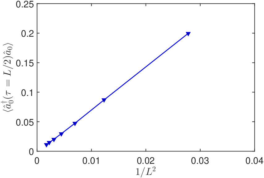
Fig. 13 shows that adopting a scaling and considering provides confirmation of the above law.
At the Gross-Neveu critical point, the scaling dimension of the fermion operator will be enhanced by half the fermion anomalous dimension, , such that at this critical point we expect:
| (49) |
in two spatial dimensions.
References
- Hertz (1976) J. A. Hertz, Phys. Rev. B 14, 1165 (1976).
- Millis (1993) A. J. Millis, Phys. Rev. B 48, 7183 (1993).
- Xu and Grover (2020) X. Y. Xu and T. Grover, “Competing nodal d-wave superconductivity and antiferromagnetism: a quantum monte carlo study,” (2020), arXiv:2009.06644 [cond-mat.str-el] .
- Otsuka et al. (2020) Y. Otsuka, K. Seki, S. Sorella, and S. Yunoki, Phys. Rev. B 102, 235105 (2020).
- Assaad and Herbut (2013) F. F. Assaad and I. F. Herbut, Phys. Rev. X 3, 031010 (2013).
- Otsuka et al. (2016) Y. Otsuka, S. Yunoki, and S. Sorella, Phys. Rev. X 6, 011029 (2016).
- Parisen Toldin et al. (2015) F. Parisen Toldin, M. Hohenadler, F. F. Assaad, and I. F. Herbut, Phys. Rev. B 91, 165108 (2015).
- Neto et al. (2009) A. H. C. Neto, F. Guinea, N. M. R. Peres, K. S. Novoselov, and A. K. Geim, Rev. Mod. Phys. 81, 109 (2009).
- Herbut et al. (2009a) I. F. Herbut, V. Juričić, and O. Vafek, Phys. Rev. B 80, 075432 (2009a).
- Vojta et al. (2000) M. Vojta, Y. Zhang, and S. Sachdev, Phys. Rev. Lett. 85, 4940 (2000).
- Kim et al. (2008) E.-A. Kim, M. J. Lawler, P. Oreto, S. Sachdev, E. Fradkin, and S. A. Kivelson, Phys. Rev. B 77, 184514 (2008).
- Herbut et al. (2009b) I. F. Herbut, V. Juričić, and B. Roy, Phys. Rev. B 79, 085116 (2009b).
- Ryu et al. (2009) S. Ryu, C. Mudry, C.-Y. Hou, and C. Chamon, Phys. Rev. B 80, 205319 (2009).
- Hasenbusch (2010) M. Hasenbusch, Phys. Rev. B 82, 174433 (2010).
- Campostrini et al. (2002) M. Campostrini, M. Hasenbusch, A. Pelissetto, P. Rossi, and E. Vicari, Phys. Rev. B 65, 144520 (2002).
- Kos et al. (2016) F. Kos, D. Poland, D. Simmons-Duffin, and A. Vichi, Journal of High Energy Physics 2016, 36 (2016).
- Blankenbecler et al. (1981) R. Blankenbecler, D. J. Scalapino, and R. L. Sugar, Phys. Rev. D 24, 2278 (1981).
- Hirsch (1985) J. E. Hirsch, Phys. Rev. B 31, 4403 (1985).
- White et al. (1989) S. White, D. Scalapino, R. Sugar, E. Loh, J. Gubernatis, and R. Scalettar, Phys. Rev. B 40, 506 (1989).
- Assaad and Evertz (2008) F. Assaad and H. Evertz, in Computational Many-Particle Physics, Lecture Notes in Physics, Vol. 739, edited by H. Fehske, R. Schneider, and A. Weiße (Springer, Berlin Heidelberg, 2008) pp. 277–356.
- Lang and Läuchli (2019) T. C. Lang and A. M. Läuchli, Phys. Rev. Lett. 123, 137602 (2019).
- Huffman and Chandrasekharan (2020) E. Huffman and S. Chandrasekharan, Phys. Rev. D 101, 074501 (2020).
- He et al. (2018) Y.-Y. He, X. Y. Xu, K. Sun, F. F. Assaad, Z. Y. Meng, and Z.-Y. Lu, Phys. Rev. B 97, 081110 (2018).
- Liu et al. (2020) Y. Liu, W. Wang, K. Sun, and Z. Y. Meng, Phys. Rev. B 101, 064308 (2020).
- Liu et al. (2019) Y. Liu, Z. Wang, T. Sato, M. Hohenadler, C. Wang, W. Guo, and F. F. Assaad, Nature Communications 10, 2658 (2019).
- Kane and Mele (2005) C. L. Kane and E. J. Mele, Phys. Rev. Lett. 95, 226801 (2005).
- Senthil et al. (2004a) T. Senthil, L. Balents, S. Sachdev, A. Vishwanath, and M. P. A. Fisher, Phys. Rev. B 70, 144407 (2004a).
- Senthil et al. (2004b) T. Senthil, A. Vishwanath, L. Balents, S. Sachdev, and M. P. A. Fisher, Science 303, 1490 (2004b).
- Grover and Senthil (2008) T. Grover and T. Senthil, Phys. Rev. Lett. 100, 156804 (2008).
- Bercx et al. (2017) M. Bercx, F. Goth, J. S. Hofmann, and F. F. Assaad, SciPost Phys. 3, 013 (2017).
- Collaboration et al. (2021) A. Collaboration, F. F. Assaad, M. Bercx, F. Goth, A. G?tz, J. S. Hofmann, E. Huffman, Z. Liu, F. P. Toldin, J. S. E. Portela, and J. Schwab, “The alf (algorithms for lattice fermions) project release 2.0. documentation for the auxiliary-field quantum monte carlo code,” (2021), arXiv:2012.11914 [cond-mat.str-el] .
- Wu and Zhang (2005) C. Wu and S.-C. Zhang, Phys. Rev. B 71, 155115 (2005).
- Wang et al. (2020) Z. Wang, Y. Liu, T. Sato, M. Hohenadler, C. Wang, W. Guo, and F. F. Assaad, “Doping-induced quantum spin hall insulator to superconductor transition,” (2020), arXiv:2006.13239 [cond-mat.str-el] .
- Kaul (2015) R. K. Kaul, Phys. Rev. Lett. 115, 157202 (2015).
- Chakravarty et al. (1988) S. Chakravarty, B. I. Halperin, and D. R. Nelson, Phys. Rev. Lett. 60, 1057 (1988).
- Janssen et al. (2018) L. Janssen, I. F. Herbut, and M. M. Scherer, Phys. Rev. B 97, 041117 (2018).
- Li et al. (2017) Z.-X. Li, Y.-F. Jiang, S.-K. Jian, and H. Yao, Nature Communications 8, 314 (2017).
- Otsuka et al. (2018) Y. Otsuka, K. Seki, S. Sorella, and S. Yunoki, Phys. Rev. B 98, 035126 (2018).
- Ippoliti et al. (2018) M. Ippoliti, R. S. K. Mong, F. F. Assaad, and M. P. Zaletel, Phys. Rev. B 98, 235108 (2018).
- Wang et al. (2021) Z. Wang, M. P. Zaletel, R. S. K. Mong, and F. F. Assaad, Phys. Rev. Lett. 126, 045701 (2021).
- Roy and Juričić (2019) B. Roy and V. Juričić, Phys. Rev. B 99, 241103 (2019).
- Torres et al. (2020) E. Torres, L. Weber, L. Janssen, S. Wessel, and M. M. Scherer, Phys. Rev. Research 2, 022005 (2020).
- Sato et al. (2017) T. Sato, M. Hohenadler, and F. F. Assaad, Phys. Rev. Lett. 119, 197203 (2017).
- Sato et al. (2020) T. Sato, M. Hohenadler, T. Grover, J. McGreevy, and F. F. Assaad, “Topological terms on topological defects: a quantum monte carlo study,” (2020), arXiv:2005.08996 [cond-mat.str-el] .
- Li et al. (2019) Z.-X. Li, S.-K. Jian, and H. Yao, “Deconfined quantum criticality and emergent so(5) symmetry in fermionic systems,” (2019), arXiv:1904.10975 [cond-mat.str-el] .
- Buividovich et al. (2018) P. Buividovich, D. Smith, M. Ulybyshev, and L. von Smekal, Phys. Rev. B 98, 235129 (2018).
- Zerf et al. (2017) N. Zerf, L. N. Mihaila, P. Marquard, I. F. Herbut, and M. M. Scherer, Phys. Rev. D 96, 096010 (2017).
- Knorr (2018) B. Knorr, Phys. Rev. B 97, 075129 (2018).
- Janssen and Herbut (2014) L. Janssen and I. F. Herbut, Phys. Rev. B 89, 205403 (2014).
- Shi and Zhang (2016) H. Shi and S. Zhang, Phys. Rev. E 93, 033303 (2016).
- Duane et al. (1987) S. Duane, A. D. Kennedy, B. J. Pendleton, and D. Roweth, Phys. Lett. B195, 216 (1987).
- Beyl et al. (2018) S. Beyl, F. Goth, and F. F. Assaad, Phys. Rev. B 97, 085144 (2018).
- Ulybyshev et al. (2019) M. Ulybyshev, N. Kintscher, K. Kahl, and P. Buividovich, Computer Physics Communications 236, 118 (2019).
- Hirsch (1983) J. Hirsch, Phys. Rev. B 28, 4059 (1983).
- Peskin and Schroeder (1995) M. E. Peskin and D. V. Schroeder, An introduction to quantum field theory (Westview, Boulder, CO, 1995) includes exercises.
- Seki et al. (2019) K. Seki, Y. Otsuka, S. Yunoki, and S. Sorella, Phys. Rev. B 99, 125145 (2019).