Multi-wavelength View of the Type IIn Zoo: Optical to X-ray Emission Model of Interaction-Powered SupernovaeJournal: ApJ

We consider a core-collapse SN occurring in a dense CSM. When the SN ejecta collide with the CSM, two shocks are formed; a forward shock (FS) separating the shocked and unshocked CSM and a reverse shock (RS) separating the shocked and unshocked SN ejecta (Chevalier 1982). The interface of the shocked CSM and SN ejecta is called a contact discontinuity (see Fig. 1). We consider the case where homologously expanding cold SN ejecta with a power-law density profile ($\rho_{\rm ej}\propto v^{-n}$ with $n>5$) run through a CSM of a wind density profile

where constants $\dot{M}$ and $v_{w}$ are respectively the mass loss rate and wind velocity. We adopt a normalization parameter for the density $(\dot{M}/v_{w})_{*}=10^{-4}M_{\odot}{\rm yr^{-1}}/({\rm km\ s^{-1}})$. The number density and velocity at the immediate downstream can be obtained from the self-similar solution of the shock dynamics (Chevalier 1982). The details of shock propagation are described in Appendix A. We here overview how the dissipated kinetic energy at these shocks are converted to radiation and how the radiation emanates from the CSM.

The immediate upstream, either the unshocked ejecta or unshocked CSM, is a cold but ionized gas due to strong UV/X-ray emission from the shocked region. When this crosses the shock, thermal relaxations between particles of the same species first occur; for a gas of density $\rho$ the electron-electron and proton-proton collision timescales (Padmanabhan 2000),

are generally much shorter than the dynamical timescales,

Here $k_{\rm B}$ is the Boltzmann constant, $m_{e}(m_{p})$ is the electron (proton) mass, $e$ is the electron charge, and $\ln\Lambda\approx 30$ is the Coulomb logarithm. Then the temperature $T_{\mathrm{e}}$ ($T_{\mathrm{p}}$) of electrons (protons) at the immediate downstream of shock fronts is obtained as functions of the shock velocities $v_{\rm fs(rs)}$ from the jump condition with an adiabatic index $\gamma=5/3$ as

Most of the energy dissipated at the shock goes to protons at the immediate downstream.

The FS (RS) downstream is slightly slower (faster) than the contact discontinuity, so for both shocks the incoming gas is gradually advected to the contact discontinuity. The advection timescale is roughly equivalent to the dynamical timescale $t_{\rm ad}\approx t_{\mathrm{dyn}}$ ¹¹ 1 The width of the downstream is compressed by a factor $(\gamma+1)/(\gamma-1)$, but from the jump condition the downstream velocity in the shock rest frame is reduced by the same factor with respect to the upstream velocity.. During the advection, the electrons in the shocked region exchange their energies with the protons due to Coulomb interaction with an equipartition timescale of

The electrons also either gain or lose energy by emitting or absorbing photons via bremsstrahlung processes and by inelastic Compton scattering (Weaver 1976; Katz et al. 2010). Since the timescales in equations (2) and (3) are shorter than equation (7) and other relevant cooling and heating timescales, the shocked regions can be treated as two temperature plasmas. On the other hand, since the advection of the shocked plasma (equation 4) is the slowest process, we can approximate that the radiative shock structure is quasi-steady. For each epoch we obtain the hydrodynamic parameters at the shock interface (shock radius, velocity and upstream density), and use these to solve the electron/proton temperatures inside each region swept by the FS and RS.

Photons are predominantly generated by bremsstrahlung at the immediate shock downstream of the FS and RS. The spectral energy distributions are modified by Compton scattering and free-free and bound-free absorption while propagating through the shocked regions. Radiation escapes from both regions after a diffusion time passes, and half of the radiation that escapes the FS region reaches the observer (see Fig. 1). We solve the radiation transfer to calculate the escaping photon spectrum consistently with the two temperature structure in the shocked regions.

In this section, we review the basic equations that govern the structure of the shocked region.

As the scale heights of the downstream parameters are much smaller than $r$, the geometric factor $r^{2}$ can be treated as a constant in the narrow shocked region. Assuming a steady state in the shock rest frame the hydrodynamic equations are described as (e.g. Takei & Shigeyama 2020)

where $\rho$ is the mass density of the shock downstream, and the pressure $p$ and specific internal energy $U$ are defined as

where $x$ is the ionization fraction. We set $x=1$ when protons and electrons have not reached equipartition yet. Once $T_{e}=T_{p}$, assuming local thermodynamic equilibrium the value of $x$ can be obtained from the Saha equation. The gas is assumed to consist purely of hydrogen for simplicity, with the temperature of neutral and ionized hydrogen are assumed to be equal, $T_{\rm HI}=T_{p}$, in the entire shocked region. $F_{\nu}$ and $e_{\mathrm{rad},\nu}$ are the energy flux and density of radiation, respectively. Flux-limited diffusion (e.g. Levermore & Pomraning 1981) gives the flux as a function of $e_{\rm rad,\nu}$ by the following equation

where $\kappa_{\nu}$ is the opacity, $c$ is the speed of light, and $\lambda_{\nu}$ is a parameter between 0 and 1/3, the limits corresponding to the optically thin and thick case respectively.

When electrons and protons have different temperatures, the Coulomb interaction works between them to reduce the difference. The energy exchange rate of protons and electrons $P_{\rm e-p}$ [erg/cm³/s] is (Katz et al. 2011)

where $n_{i}=x\rho/m_{p}$ is the number density of protons and electrons, and $\sigma_{T}$ is the Thomson cross section. Noting that electrons are dominantly affected by the photon field, the energy equation can be rewritten into the following equations for $T_{e}$ and $T_{p}$

The equation of radiation transfer in spherical symmetry along the advection flow of the downstream plasma is

where $I_{\nu}$ is the specific intensity, $\theta$ is the angle between the light ray’s propagation direction and the radial direction, and

are respectively the emissivity and absorption coefficient, which are related to the free-free and Comptonization processes. Taking the zeroth moment of equation (17) we obtain

Here we have neglected a geometric factor $2F_{\nu}/r$ because the relevant scale lengths are much shorter than the radius $r$. Transferring to the Euler description and in the shock’s rest frame, $\partial/\partial t\to(\partial/\partial t+v\partial/\partial r)$. From the steady state assumption we obtain

For simplicity we assume free-free is the dominant emission/absorption processes and neglect free-bound/bound-free and bound-bound contributions. The emissivity [erg/s/cm³/Hz] and absorption coefficient [cm^-1] are given in cgs units by (Rybicki & Lightman 1979)

where $h$ is Planck’s constant and $g_{\rm ff}$ is the Gaunt factor

For the photon frequency we sample a wide range of 0.1 eV$<h\nu<100$ MeV, with 80 bins evenly spaced on a logarithmic scale.

For inverse-Compton scattering, we obtain the rate of change in photon energy density $j_{\nu,\rm IC}$ [erg/s/cm³/Hz] as

where $\sigma_{\rm KN}(\nu)$ is the Klein-Nishina cross section given by (Rybicki & Lightman 1979)

with $\beta=h\nu/m_{e}c^{2}$, and $\nu^{\prime}(\nu,T_{e})$ is the typical frequency of photons whose frequency becomes $\nu$ after scattering.

For a non-relativistic electron ($k_{\rm B}T_{e}\ll m_{e}c^{2}$) and a photon energy $h\nu^{\prime}\ll m_{e}c^{2}$, the typical frequency $\nu$ after scattering of a photon of energy $\nu^{\prime}$ is (Rybicki & Lightman 1979)

Since we consider a photon spectrum at high energies exceeding $m_{e}c^{2}$ as well, we refine the second term as follows. For a photon scattering with an electron at rest, from the kinematics of the scattering

where $\theta$ is the angle between the momenta of scattered and incident photons. Averaging over $\theta$

Repeating the same argument that led to equation (26), we obtain

The factor 4 is valid only when electrons are non-relativistic, which is generally satisfied for our model parameters. For each $\nu$ we solve equation (27) implicitly and obtain $\nu^{\prime}$.

By solving equations (8), (9), (13), (15), (16) and (21) for both the forward and reverse shock regions, one can in principle obtain the shock structure, i.e., $T_{\mathrm{e}}(r)$, $T_{\mathrm{p}}(r)$, $\rho(r)$, $v(r)$, $F_{\nu}(r)$ and $e_{\rm rad,\nu}(r)$. These equations take into account the radiation feedback onto the dynamics of the advected gas, but this will be self-consistent only if the propagation of the shock is simultaneously modified (Takei & Shigeyama 2020). Our formulation relies on the self-similar solution for the shock propagation and parameters at the immediate downstream, and taking into account the deviation from this self-similar evolution drastically complicates the problem.

In order to simplify the problem, in this work we adopt an assumption that the pressure gradient is zero in each shocked region, i.e. the dynamics is assumed to be one-zone. The plasma that crosses the shock is thus advected by a constant advection velocity, given by the downstream velocity in the shock’s rest frame. Takei & Shigeyama 2020, which solved the above equations with the assumption of local thermodynamic equilibrium in the shocked region and adopting the diffusion approximation, shows that a nearly constant pressure is indeed seen (see their Figure 1).

On the other hand we follow the evolution of $T_{e},T_{p}$ and $e_{\rm rad,\nu}$ in the region, which are important for the emission. With our assumption the energy equation (10) is simplified to

Under the one-zone assumption, we average the flux that appears in the energy equation, over the shocked region’s volume. The volume average then becomes a surface integral, and the energy equation is modified as

where $e_{\rm esc,\nu}$ [${\rm erg/cm^{3}/Hz}$] is the energy density of radiation taken away from the shocked region, and $j_{\nu,\rm in}$ is the source term which consists of two components explained later in this section. From our constant pressure assumption $v$ is independent of $r$, and we can set $vd/dr=d/dt$, where $t$ is the time passed for the downstream plasma from when it crossed the shock. Then while $T_{p}>T_{e}$, the equations for $T_{e}$ and $T_{p}$ are

We make $T_{e}$ and $T_{p}$ equal by hand (with the total energy conserved) if these two approach within 10%. This is merely for numerical purpose, as a finite difference tends to make the Coulomb term $P_{\rm e-p}$ erroneously large after electrons and protons have cooled down. Once $T_{e}=T_{p}$, thermal relaxation is fast enough that this equality is kept. Then the equations for $T_{e}$ and $T_{p}$ are further simplified to

We first obtain $[1+x(T_{e})]T_{e}$ with this equation, then use the Saha equation and implicitly obtain $T_{e}(=T_{p})$.

We next present our method of obtaining $e_{\rm rad,\nu},e_{\rm esc,\nu}$. The equation for radiation transfer becomes

where we redefined $j_{\nu}\equiv j_{\nu,\rm ff}+j_{\nu,\rm in}$. This equation reduces to the standard equation of radiation transfer if $\dot{e}_{\rm esc,\nu}=0$ is assumed. In this case the formal solution can be obtained by expressing $e_{\rm rad,\nu}$ as $e_{\rm rad,\nu}(t)=F(t)\exp[-\int^{t}_{0}ds\ \alpha^{\prime}_{\nu}(s)c]$, and solving for $F(t)$ by substituting this into equation (33).

To determine $\dot{e}_{\rm rad,\nu}$ and $\dot{e}_{\rm esc,\nu}$ separately we need another constraint, which should be related to the physics of diffusion. As an approximation we treat the diffusion as a hard cutoff over a typical diffusion timescale $t_{\rm diff}$. In other words, photons created at time $t=s$ are in the shocked region and contribute to $e_{\rm rad,\nu}$ at time $s<t<s+t_{\rm diff}$, then completely escape and contribute to $e_{\rm esc,\nu}$ at $t>s+t_{\rm diff}$. Then by analogy of the standard case described above, we find the solution of the form

for $t>t_{\rm diff}$, and

for $0<t\leq t_{\rm diff}$. To calculate the integrals, we keep records of $j_{\rm\nu}$ and $\alpha^{\prime}_{\rm\nu}$ throughout the dynamical time with timestep $t_{\rm dyn}/24000$. This resolution is limited by our computational resource. In the RS region, we observed cases where the cooling timescale (equation 48) became shorter than this time resolution, thereby preventing us to obtain these integrals accurately. In these cases we switched to an analytical treatment for calculating $e_{\rm rad,\nu}$ and $e_{\rm esc,\nu}$, explained in Appendix B.

We calculate $T_{e},T_{p},e_{\rm rad,\nu},$ and $e_{\rm esc,\nu}$ from $t=0$ to $t_{\rm end}$, the timescale for the gas to be advected from the shock to the contact discontinuity, in our case equivalent to the dynamical time (see Section II.1). Thus $t_{\rm end}$ is roughly equivalent to the epoch $\mathcal{T}$, or time from explosion²² 2 This is not to be confused with the variable $t$, which was previously defined for the calculation of the shock structure at a given epoch $\mathcal{T}$.. We do this integration for a series of epochs $\{\mathcal{T}_{0},\mathcal{T}_{1},\cdots\}$, with $t_{\rm end,N}=\mathcal{T}_{N}\ (N=0,1,\cdots)$. For each epoch the conditions at $t=0$ (i.e. at the shock) are obtained by the equations in Appendix A. The series should be set so that the dynamics and radiation flow do not significantly change between neighboring epochs. We set the epochs by the following equations

The parameter $\mathcal{T}_{\rm CSM}$ is the diffusion timescale in the CSM which controls the light curve evolution

where $\kappa_{\rm scat}\approx 0.34\ {\rm cm^{2}\ g^{-1}}$ is the Thomson scattering opacity. The series continues up to 250 days or when the RS sweeps the entire outer ejecta, whichever is earlier. Variables $t^{\rm RS}_{\rm diff},t^{\rm FS}_{\rm diff}$ are respectively the diffusion timescales in the RS and FS region. The diffusion time in the FS region $t^{\rm FS}_{\rm diff}$ is given by its optical depth multiplied by the light-crossing timescale

where the width of the FS region $\Delta r_{\rm FS}$ relates to the radius of the contact discontinuity $r_{\rm sh}$ derived in equation (A6) as $\Delta r_{\rm FS}\approx[(\gamma-1)/(\gamma+1)]r_{\rm sh}$. The diffusion time in the RS region $t^{\rm RS}_{\rm diff}$ depends on the parameters for the self-similar solution, but is generally much shorter than $t^{\rm FS}_{\rm diff}$ due to the much smaller width. For example if we assume $n=10$ and $\gamma=4/3$, we find $t^{\rm RS}_{\rm diff}\approx 0.134t^{\rm FS}_{\rm diff}$.

In our model $j_{\nu,\rm in}$ has two components. One is radiation entering from the other shocked region, shown as black arrows in Figure 1. For radiation escaping from the FS region, assuming the escaping radiation is isotropic $r_{\rm fs}^{2}/(r_{\rm sh}^{2}+r_{\rm fs}^{2})\approx 1/2$ escapes outwards (which is observed), while the other 1/2 goes inwards to the RS region, and is possibly reprocessed there. Under the assumption of cold SN ejecta in which only the vicinity of the shocked region is ionized, we assume that the bulk of the ejecta are transparent and all the escaping radiation from the RS region goes to the FS region as a source term. We calculate the source term from the $e_{\rm esc,\nu}$ in the previous epoch, and inject this at a constant rate for $t_{\rm dyn}$.

The other component, which is rather artificial, is $e_{\rm rad,\nu}$ that should be present in the shocked region at $t=0$. Our formulation of $e_{\rm rad,\nu}$ (equation 36) implicitly assumes $e_{\rm rad,\nu}=0$ at $t=0$, which neglects this contribution. We instead include this as a source term estimated from the previous epoch; i.e. the leftover $e_{\rm rad,\nu}$ in the end of the previous epoch, $e_{\rm rad,\nu}(t=t_{\rm end,N-1})$, is carried over in the present epoch $\mathcal{T}_{N}$ as a source term. We inject this at constant rate for the first diffusion time at epoch $\mathcal{T}_{N}$.

When setting the injection term from the previous epoch, we make sure that the total injected energy in the shocked region, $e_{\rm esc,\nu}$ (or $e_{\rm rad,\nu}$) times the volume of the shocked region, is conserved. Mathematically, $j_{\rm\nu,in}$ is given for the FS and RS regions as

where $\Theta(t)$ is the Heaviside step function, and $V^{\rm FS(RS)}_{N}$ is the volume of the FS (RS) region at epoch $\mathcal{T}_{N}$. Variables with superscript FS (RS) denote values in the FS (RS) region. In the self-similar solution the ratio of the volumes of the FS and RS regions is a constant of time. We neglect additional energy sources that can appear as a source term, such as radioactive decay of nickel inside the ejecta.

For the first epoch $\mathcal{T}_{0}$, the calculation is iterated until $e_{\rm rad,\nu}$ becomes stable. To obtain $j_{\rm\nu,in}$ for the next iteration, we use the values of $e_{\rm rad,\nu}$ and $e_{\rm esc,\nu}$ at $t=t_{\rm end,0}$ because there is no previous epoch. The energy density at $t=t_{\rm end,0}$ becomes stable within 1% after about 10 iterations, from which we move on to epoch $\mathcal{T}_{1}$.

To obtain the observed spectrum, we need to solve the radiation transfer through the unshocked CSM. At each epoch, the luminosity of radiation that escapes from the FS region towards the observer is

where the factor 1/2 is due to the aforementioned geometrical effect. Once we obtain this luminosity $L_{\nu}$, we use version 17.02 of CLOUDY (Ferland et al. 2017) to obtain the spectrum after being processed through the unshocked CSM $L_{\rm\nu,CSM}$. We assume the CSM extends with a spherically symmetric wind profile from $r=r_{\rm sh}$ out to $10^{17}$ cm. The metallicity of the CSM is assumed to be solar.

This treatment also assumes a steady state, i.e. the photoionization at a given epoch is determined by the luminosity at that time. For Type IIn SNe this is justified, as the recombination timescale is generally much shorter than the dynamical timescale (Chevalier & Irwin 2012). For example, for a gas of $T_{e}\sim 10^{4}$ K the recombination coefficient is $\alpha_{\rm rec}\sim O(10^{-13})\ {\rm cm^{3}\ s^{-1}}$, and the recombination timescale is of order $10^{3}$ ($10^{5}$) s at day 10 (100) for our fiducial model parameters.

We also include the effect of diffusion inside the CSM delaying the light curve, by the following formula (Chatzopoulos et al. 2012; equation 4)

For the contribution of $L_{\nu,\rm CSM}$ at $t<\mathcal{T}_{0}$, which is absent in our modelling, we adopt the value at $t=\mathcal{T}_{0}$ for simplicity. The actual contribution is uncertain, as this also depends on when the CSM interaction starts. However, the exponential dependence makes this uncertainty unimportant after about a few times $\mathcal{T}_{\rm CSM}$.

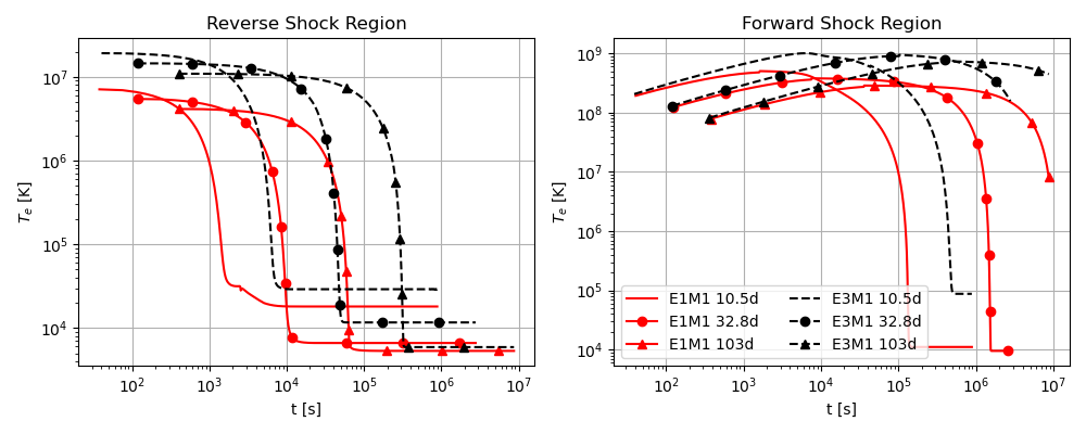
We show the change of electron temperature $T_{e}$ as a function of time in Figure 2. The value of $T_{e}$ initially rises due to Coulomb interaction with the protons (hotter by $m_{p}/m_{e}$), but then the temperature drops first due to free-free emission, then by inverse Compton scattering. The detailed evolution differs for RS and FS, which we discuss in detail below.

Figure 4 shows the resulting spectra of photons escaping the FS region for our choice of model parameters. We find that for the E1M1 and all the M10 models soft X-rays emitted from the shock are significantly absorbed by the unshocked CSM, and the observed spectrum is much different from the spectrum emergent from the shock front. A fraction of the absorbed X-ray photons are converted to optical and UV emission, with a large number of emission lines including H$\alpha$ at $\approx 1.9$ eV. This matches with the naive expectation that for low $E_{\rm ej}$ and/or high $\dot{M}/v_{w}$, the shock expands slower and the optical depth of the CSM is kept high. On the other hand, the observed spectra for models E3M1 and E10M1 are largely unmodified from the spectrum from the shock. In addition to the CSM quickly becoming optically thin, larger explosion energies (hence larger shock velocity) extend the FS spectra to hard X-rays, which avoid significant absorption by the CSM.

An important aspect that determines the spectrum from the shock is the optical depth to Thomson scattering inside the FS region. For a wind profile CSM this is equivalent to that in the unshocked CSM, and is given as

where we assumed $\kappa_{\rm scat}=0.34\ {\rm cm^{2}g^{-1}}$.

For an optically thick ($\tau_{\rm fs}\gg 1$) case, Compton downscattering can drastically reduce the photon energy. The number of Thomson scatterings per unit time is $\kappa_{\rm scat}\times 7\rho_{\rm w}c$, and photons stay in the FS region for a diffusion time $t_{\rm diff,fs}\sim\kappa_{\rm scat}\rho_{\rm w}r_{\rm sh}^{2}/7c$, where the factor 7 comes from the compression ratio for adiabatic index $4/3$. Thus there are $\tau_{\rm fs}^{2}$ scatterings in the FS region before escaping, and as a result the energy of photons reaching the observer is reduced to $\approx 511{\rm keV}/\tau_{\rm fs}^{2}\sim 0.3\ {\rm keV}(\tau_{\rm fs}/40)^{-2}$. This is consistent with the cutoff in the spectra at the FS for the E1M10 model on day 10.6, when $\tau_{\rm fs}\approx 38$ (blue dotted line in the top-right panel of Figure 4).

The degree of absorption of soft X-rays depends on this cutoff frequency and the luminosity of ionizing photons $L_{\rm ion}$, as discussed in Chevalier & Irwin 2012. Qualitatively, in order for soft X-rays to reach the observer the following two conditions must be satisfied; (i) $\tau_{\rm fs}$ should be at most a few tens, so that the cutoff is in or beyond the soft X-ray band (ii) the flux of ionizing photons is high enough that the main elements that contribute to absorption of soft X-rays (oxygen and iron) are completely ionized. The latter is quantified as the ionization parameter $\xi\equiv L_{\rm ion}/(nr^{2})\approx 4\pi m_{p}L_{\rm ion}/(\dot{M}/v_{w})$ in cgs units. Chevalier & Irwin 2012 finds that $\xi$ greater than $5000$–$10^{4}$ will ionize all the elements, a precise value depending on the characteristic temperature of the spectrum. For our parameters

which is consistent with our results within an order of magnitude, and explains the tendency seen in our spectra that models with larger $E_{\rm ej}$ (i.e. larger $L_{\rm ion}$) and smaller $\dot{M}/v_{w}$ are visible in soft X-rays.

Another notable feature is that the spectrum $\nu L_{\nu}$ below the cutoff is nearly flat for the E1M1 and E3M1 cases, while it becomes steeper up to $\nu L_{\nu}\propto\nu$ for the E10M1 case. The latter is simply from the fact that the free-free emissivity $j_{\nu,\rm ff}$ is flat at $h\nu\ll k_{\rm B}T_{e}$, and Compton and IC scatterings are ineffective. Repeated scattering between electrons and photons can convert X-ray photons to lower energies, which flattens the spectrum from the free-free one.

We calculate the optical and X-ray light curves to compare with observations. For the optical light curves, we use the $\nu L_{\nu}$ from our model and adopt the Johnson-Cousins filter response function to obtain the (absolute) B and V band magnitudes with

where $e(\lambda)$ is the filter response function for each band³³ 3 https://www.aip.de/en/research/facilities/stella/instruments/data, $f_{\nu,\rm ref}$ is the reference flux that defines the zero point, and we used the conversion $f_{\lambda}=(c/\lambda^{2})f_{\nu}$. For $f_{\nu,\rm ref}$ we adopt the values $4260$ Jy and $3640$ Jy for the B and V bands respectively (see Table IV of Bessell 1979). The resulting light curves in B and V bands are shown in Figure 5. The peak magnitude of average Type IIn SNe is estimated to be $M_{V}=-18.4\pm 1.0$ (Kiewe et al. 2012), with more recent estimates (Richardson et al. 2014; Nyholm et al. 2020) giving consistent results. Our results that roughly reproduced this magnitude favors mass-loss rates of order $0.1M_{\odot}\ {\rm yr}^{-1}$. This is at odds with the much lower $\dot{M}$ derived for some SNe IIn in previous works (Kiewe et al. 2012; Taddia et al. 2013). This should be partly due to the shortcomings of our model with incomplete opacity in the shocked region and an assumption of a one-zone density profile, which are elaborated in Section V. The discrepancy can also be from their assumption of a high conversion efficiency from kinetic energy dissipation rate to H$\alpha$ luminosity, $\epsilon_{\rm H\alpha}=0.1$. Inspecting Figure 4, some spectra show $\epsilon_{\rm H\alpha}\ll 0.1$, especially for the M1 models. A low $\epsilon_{\rm H\alpha}$ is also implied from a more recent SN IIn sample (Kokubo et al. 2019). As the value of $\dot{M}$ derived from this method scales as the inverse of $\epsilon_{\rm H\alpha}$, this implies that the actual $\dot{M}$ can be much higher than previously estimated. A more sophisticated modelling of $\epsilon_{\rm H\alpha}$ may give a better understanding on $\dot{M}$, although it is beyond the scope of this work.

References

- Balberg & Loeb (2011) Balberg, S. & Loeb, A. 2011, MNRAS, 414, 1715
- Bessell (1979) Bessell, M. S. 1979, PASP, 91, 589
- Bietenholz et al. (2018) Bietenholz, M. F., Kamble, A., Margutti, R., Milisavljevic, D., & Soderberg, A. 2018, MNRAS, 475, 1756
- Blandford & Eichler (1987) Blandford, R. & Eichler, D. 1987, Phys. Rep., 154, 1
- Chandra (2018) Chandra, P. 2018, Space Sci. Rev., 214, 27
- Chandra et al. (2012a) Chandra, P., Chevalier, R. A., Chugai, N., Fransson, C., Irwin, C. M., Soderberg, A. M., Chakraborti, S., & Immler, S. 2012a, ApJ, 755, 110
- Chandra et al. (2015) Chandra, P., Chevalier, R. A., Chugai, N., Fransson, C., & Soderberg, A. M. 2015, ApJ, 810, 32
- Chandra et al. (2012b) Chandra, P., Chevalier, R. A., Irwin, C. M., Chugai, N., Fransson, C., & Soderberg, A. M. 2012b, ApJ, 750, L2
- Chatzopoulos et al. (2012) Chatzopoulos, E., Wheeler, J. C., & Vinko, J. 2012, ApJ, 746, 121
- Chevalier (1982) Chevalier, R. A. 1982, ApJ, 258, 790
- Chevalier & Fransson (2003) Chevalier, R. A. & Fransson, C. 2003, Supernova Interaction with a Circumstellar Medium, ed. K. Weiler, Vol. 598, 171–194
- Chevalier & Irwin (2011) Chevalier, R. A. & Irwin, C. M. 2011, ApJ, 729, L6
- Chevalier & Irwin (2012) —. 2012, ApJ, 747, L17
- Chugai (1991) Chugai, N. N. 1991, MNRAS, 250, 513
- Dwarkadas et al. (2016) Dwarkadas, V. V., Romero-Cañizales, C., Reddy, R., & Bauer, F. E. 2016, MNRAS, 462, 1101
- Ferland et al. (2017) Ferland, G. J., Chatzikos, M., Guzmán, F., Lykins, M. L., van Hoof, P. A. M., Williams, R. J. R., Abel, N. P., Badnell, N. R., Keenan, F. P., Porter, R. L., & Stancil, P. C. 2017, Rev. Mexicana Astron. Astrofis., 53, 385
- Filippenko (1997) Filippenko, A. V. 1997, Annual Review of Astronomy and Astrophysics, 35, 309
- Förster et al. (2018) Förster, F., Moriya, T. J., Maureira, J. C., Anderson, J. P., Blinnikov, S., Bufano, F., Cabrera-Vives, G., Clocchiatti, A., de Jaeger, T., Estévez, P. A., Galbany, L., González-Gaitán, S., Gräfener, G., Hamuy, M., Hsiao, E. Y., Huentelemu, P., Huijse, P., Kuncarayakti, H., Martínez, J., Medina, G., Olivares E., F., Pignata, G., Razza, A., Reyes, I., San Martín, J., Smith, R. C., Vera, E., Vivas, A. K., de Ugarte Postigo, A., Yoon, S. C., Ashall, C., Fraser, M., Gal-Yam, A., Kankare, E., Le Guillou, L., Mazzali, P. A., Walton, N. A., & Young, D. R. 2018, Nature Astronomy, 2, 808
- Fransson et al. (2014) Fransson, C., Ergon, M., Challis, P. J., Chevalier, R. A., France, K., Kirshner, R. P., Marion, G. H., Milisavljevic, D., Smith, N., Bufano, F., Friedman, A. S., Kangas, T., Larsson, J., Mattila, S., Benetti, S., Chornock, R., Czekala, I., Soderberg, A., & Sollerman, J. 2014, ApJ, 797, 118
- Grasberg & Nadezhin (1986) Grasberg, E. K. & Nadezhin, D. K. 1986, Pisma v Astronomicheskii Zhurnal, 12, 168
- Katsuda et al. (2016) Katsuda, S., Maeda, K., Bamba, A., Terada, Y., Fukazawa, Y., Kawabata, K., Ohno, M., Sugawara, Y., Tsuboi, Y., & Immler, S. 2016, ApJ, 832, 194
- Katsuda et al. (2014) Katsuda, S., Maeda, K., Nozawa, T., Pooley, D., & Immler, S. 2014, ApJ, 780, 184
- Katz et al. (2010) Katz, B., Budnik, R., & Waxman, E. 2010, ApJ, 716, 781
- Katz et al. (2011) Katz, B., Sapir, N., & Waxman, E. 2011, arXiv e-prints, arXiv:1106.1898
- Kiewe et al. (2012) Kiewe, M., Gal-Yam, A., Arcavi, I., Leonard, D. C., Emilio Enriquez, J., Cenko, S. B., Fox, D. B., Moon, D.-S., Sand , D. J., Soderberg, A. M., & CCCP, T. 2012, ApJ, 744, 10
- Kim et al. (2014) Kim, M., Zheng, W., Li, W., Filippenko, A. V., Cenko, S. B., Arbour, R., Masi, G., Nocentini, F., Schmeer, P., Zhang, J., Want, X., Tartaglia, L., Pastorello, A., Benetti, S., Cappellaro, E., Tomasella, L., Ochner, P., Elias-Rosa, N., & Turatto, M. 2014, Central Bureau Electronic Telegrams, 3777, 1
- Kokubo et al. (2019) Kokubo, M., Mitsuda, K., Morokuma, T., Tominaga, N., Tanaka, M., Moriya, T. J., Yoachim, P., Ivezić, Ž., Sako, S., & Doi, M. 2019, ApJ, 872, 135
- Levermore & Pomraning (1981) Levermore, C. D. & Pomraning, G. C. 1981, ApJ, 248, 321
- Margutti et al. (2017) Margutti, R., Kamble, A., Milisavljevic, D., Zapartas, E., de Mink, S. E., Drout, M., Chornock, R., Risaliti, G., Zauderer, B. A., Bietenholz, M., Cantiello, M., Chakraborti, S., Chomiuk, L., Fong, W., Grefenstette, B., Guidorzi, C., Kirshner, R., Parrent, J. T., Patnaude, D., Soderberg, A. M., Gehrels, N. C., & Harrison, F. 2017, ApJ, 835, 140
- Matzner & McKee (1999) Matzner, C. D. & McKee, C. F. 1999, ApJ, 510, 379
- Merloni et al. (2012) Merloni, A., Predehl, P., Becker, W., Böhringer, H., Boller, T., Brunner, H., Brusa, M., Dennerl, K., Freyberg, M., Friedrich, P., Georgakakis, A., Haberl, F., Hasinger, G., Meidinger, N., Mohr, J., Nandra, K., Rau, A., Reiprich, T. H., Robrade, J., Salvato, M., Santangelo, A., Sasaki, M., Schwope, A., Wilms, J., & German eROSITA Consortium, t. 2012, arXiv e-prints, arXiv:1209.3114
- Milisavljevic et al. (2015) Milisavljevic, D., Margutti, R., Kamble, A., Patnaude, D. J., Raymond, J. C., Eldridge, J. J., Fong, W., Bietenholz, M., Challis, P., Chornock, R., Drout, M. R., Fransson, C., Fesen, R. A., Grindlay, J. E., Kirshner, R. P., Lunnan, R., Mackey, J., Miller, G. F., Parrent, J. T., Sanders, N. E., Soderberg, A. M., & Zauderer, B. A. 2015, ApJ, 815, 120
- Moriya et al. (2013) Moriya, T. J., Maeda, K., Taddia, F., Sollerman, J., Blinnikov, S. I., & Sorokina, E. I. 2013, MNRAS, 435, 1520
- Murase (2018) Murase, K. 2018, Phys. Rev. D, 97, 081301
- Murase et al. (2019) Murase, K., Franckowiak, A., Maeda, K., Margutti, R., & Beacom, J. F. 2019, ApJ, 874, 80
- Murase et al. (2011) Murase, K., Thompson, T. A., Lacki, B. C., & Beacom, J. F. 2011, Phys. Rev. D, 84, 043003
- Murase et al. (2014) Murase, K., Thompson, T. A., & Ofek, E. O. 2014, MNRAS, 440, 2528
- Newton & Puckett (2010) Newton, J. & Puckett, T. 2010, Central Bureau Electronic Telegrams, 2532, 1
- Nyholm et al. (2020) Nyholm, A., Sollerman, J., Tartaglia, L., Taddia, F., Fremling, C., Blagorodnova, N., Filippenko, A. V., Gal-Yam, A., Howell, D. A., Karamehmetoglu, E., Kulkarni, S. R., Laher, R., Leloudas, G., Masci, F., Kasliwal, M. M., Morå, K., Moriya, T. J., Ofek, E. O., Papadogiannakis, S., Quimby, R., Rebbapragada, U., & Schulze, S. 2020, A&A, 637, A73
- Ofek et al. (2014) Ofek, E. O., Zoglauer, A., Boggs, S. E., Barriére, N. M., Reynolds, S. P., Fryer, C. L., Harrison, F. A., Cenko, S. B., Kulkarni, S. R., Gal-Yam, A., Arcavi, I., Bellm, E., Bloom, J. S., Christensen, F., Craig, W. W., Even, W., Filippenko, A. V., Grefenstette, B., Hailey, C. J., Laher, R., Madsen, K., Nakar, E., Nugent, P. E., Stern, D., Sullivan, M., Surace, J., & Zhang, W. W. 2014, ApJ, 781, 42
- Padmanabhan (2000) Padmanabhan, P. 2000, Theoretical astrophysics. Vol.1: Astrophysical processes
- Pan et al. (2013) Pan, T., Patnaude, D., & Loeb, A. 2013, MNRAS, 433, 838
- Petropoulou et al. (2016) Petropoulou, M., Kamble, A., & Sironi, L. 2016, MNRAS, 460, 44
- Richardson et al. (2014) Richardson, D., Jenkins, Robert L., I., Wright, J., & Maddox, L. 2014, AJ, 147, 118
- Rybicki & Lightman (1979) Rybicki, G. B. & Lightman, A. P. 1979, Radiative processes in astrophysics
- Schlegel (1990) Schlegel, E. M. 1990, MNRAS, 244, 269
- Smith (2014) Smith, N. 2014, ARA&A, 52, 487
- Stoll et al. (2011) Stoll, R., Prieto, J. L., Stanek, K. Z., Pogge, R. W., Szczygieł, D. M., Pojmański, G., Antognini, J., & Yan, H. 2011, ApJ, 730, 34
- Svirski et al. (2012) Svirski, G., Nakar, E., & Sari, R. 2012, ApJ, 759, 108
- Taddia et al. (2013) Taddia, F., Stritzinger, M. D., Sollerman, J., Phillips, M. M., Anderson, J. P., Boldt, L., Campillay, A., Castellón, S., Contreras, C., Folatelli, G., Hamuy, M., Heinrich-Josties, E., Krzeminski, W., Morrell, N., Burns, C. R., Freedman, W. L., Madore, B. F., Persson, S. E., & Suntzeff, N. B. 2013, A&A, 555, A10
- Takei & Shigeyama (2020) Takei, Y. & Shigeyama, T. 2020, PASJ, 72, 67
- Tsuna et al. (2019) Tsuna, D., Kashiyama, K., & Shigeyama, T. 2019, ApJ, 884, 87
- Weaver (1976) Weaver, T. A. 1976, ApJS, 32, 233
- Zhang et al. (2012) Zhang, T., Wang, X., Wu, C., Chen, J., Chen, J., Liu, Q., Huang, F., Liang, J., Zhao, X., Lin, L., Wang, M., Dennefeld, M., Zhang, J., Zhai, M., Wu, H., Fan, Z., Zou, H., Zhou, X., & Ma, J. 2012, AJ, 144, 131
- Zirakashvili & Ptuskin (2016) Zirakashvili, V. N. & Ptuskin, V. S. 2016, Astroparticle Physics, 78, 28