Determining our peculiar velocity from the aberration in the cosmic microwave backgroundDetermining our peculiar velocity from the aberration in the cosmic microwave background–2021

On the theoretical side the fluctuations in the cosmic microwave background (CMB) radiation are usually computed in the rest frame of the CMB with computer programs such as CAMB. However, on the observational side, one has to take into account our peculiar velocity with respect to the rest frame of the CMB. This leads to the large Doppler dipole contribution in the CMB on which the usual determination of our velocity is based. For further cosmological CMB analysis this contribution is ignored.

The peculiar velocity is defined as the velocity of our solar system barycentre relative to the CMB rest frame, which in turn is defined by the vanishing of the temperature dipole $a_{1m}$. These coefficients are extracted from the spherical expansion of the temperature fluctuations

where $Y_{\ell m}(\vartheta,\varphi)$ are the spherical harmonics. The COBE mission determined the peculiar velocity as $\beta_{\odot}=0.00123$ in the direction $(l,b)\simeq(264^{\circ},48^{\circ})$ in galactic coordinates (Kogut et al. 1993), where $\beta:=v/c$ is the velocity in units of the speed of light $c$.

If $T^{\text{(rest)}}$ and $\hat{n}^{\text{(rest)}}$ denote the CMB rest frame temperature and the unit vector of the considered direction, respectively, then a Lorentz transformation according to the peculiar velocity $\vec{\beta}$ leads to the transformed temperature (Challinor & van Leeuwen 2002)

in the frame of the observer, who measures $T^{\text{(obs)}}(\hat{n}^{\text{(obs)}})$ in the direction $\hat{n}^{\text{(obs)}}$ and $\gamma:=(1-\beta^{2})^{-1/2}$. It is instructive to consider this expression in linear order of $\beta$, which leads to the temperature fluctuations (see e. g. Planck Collaboration: Aghanim et al. 2014)

where $T_{0}$ denotes the CMB mean temperature. The first term on the right hand side of eq. (3) is the usual Doppler dipole which has an amplitude of $T_{0}\beta_{\odot}\simeq 3352\mu\hbox{K}$. The argument of the temperature fluctuation $\delta T^{\text{(rest)}}$ in eq. (3) is aberrated by the deflection $\nabla\hat{n}^{\text{(obs)}}\cdot\vec{\beta}$. Furthermore, this amplitude is also modulated by the factor $(1+\hat{n}^{\text{(obs)}}\cdot\vec{\beta}\,)$. The numerical analysis in this work is based on the complete formula (2) and not on the linear approximation. The angular power spectrum ${\cal D}_{\ell}=\ell(\ell+1)C_{\ell}/(2\pi)$ with $C_{\ell}=\sum_{m}|a_{\ell m}|^{2}/(2\ell+1)$ possesses for small multipole orders $2<\ell\lesssim 10$ values around $1000\mu\hbox{K}^{2}$ (Planck Collaboration: Akrami et al. 2020). Assuming that the intrinsic dipole ${\cal D}_{1}$ is of the same order, one is lead to the expectation $C_{1}=\pi{\cal D}_{1}\simeq\pi\,1000\mu\hbox{K}^{2}$ and thus to a dipole amplitude $\sqrt{C_{1}}\simeq 56\mu\hbox{K}$. An intrinsic dipole of the primordial temperature anisotropy field is therefore expected to be at the 1% level with respect to the Doppler dipole $T_{0}\beta_{\odot}$.

Although intrinsic dipole of the primordial temperature anisotropy field is considered as negligible, the observed CMB power spectrum reveals a parity asymmetry and possesses multipoles $C_{\ell}$ with enhanced power for odd multipoles $\ell$ and reduced power for the even ones for not too high values of $\ell$ corresponding to the largest angular scales (Land & Magueijo 2005; Kim & Naselsky 2010; Planck Collaboration: Akrami et al. 2020). And since the dipole is an odd multipole, of course, it could be larger than the expected 1% level.

Due to the inability to disentangle the Doppler contribution from other dipole contributions, it would thus be favourable to derive the peculiar velocity from an alternative way. This is offered by the fact that the aberration due to the peculiar velocity induces a stretching and a compression of the CMB structures in sky maps, which depends on the angular distance from the direction of our peculiar velocity, in addition to the modulation described above. These modifications of the CMB structures occur for a velocity $\beta$ of the order $10^{-3}$ at very high multipoles $\ell\gtrsim 1000$. Based on eq. (2), they are described by the aberration kernel $K_{\ell m}^{\ell^{\prime}m^{\prime}}(\beta)$ (Challinor & van Leeuwen 2002) of the multipole transformation law

where $a^{\text{(rest)}}_{\ell m}$ are the multipole expansion coefficients in the CMB rest frame and $a^{\text{(obs)}}_{\ell m}$ are those observed in the moving frame. The double sum in eq. (4) reduces to a single sum by aligning the $z$-axis of the spherical coordinate system with the direction of the velocity

which simplifies the computations drastically. This is due to the fact that in this special case the aberration causes angular distortions only in the direction of the polar angle $\vartheta$. The aberration kernel in eq. (5) can be computed by the recursion algorithm of Chluba 2011, see also (Dai & Chluba 2014).

The multipole transformation leads to a coupling between nearby multipoles. Aligning the $z$-axis of the spherical coordinate system with the boost in the forward direction, the temperature fluctuation structures are compressed towards the north pole leading to a power leakage from $C_{\ell}$ to higher multipoles $C_{\ell+1},C_{\ell+2},\dots$ on the northern hemisphere. On the southern hemisphere, the power leakage occurs towards lower multipoles $C_{\ell-1},C_{\ell-2},\dots$ since the structures are stretched there. In full sky analyses these power redistributions partly cancel, and in partial sky analyses, special care has to be taken into account (Catena & Notari 2013). Methods to detect these mode couplings between neighbouring multipoles were suggested by Burles & Rappaport 2006; Kosowsky & Kahniashvili 2011 and Amendola et al. 2011. The Planck Collaboration: Aghanim et al. 2014 finds the mode couplings to be consistent with the peculiar velocity determined by the Doppler dipole. The dependence of the magnitude of the power leakage on the angular distance from the boost direction is analysed by Jeong et al. 2014 and discussed with respect to hemispherical asymmetries by Notari et al. 2014. These considerations are extended to the polarization measurements of the CMB in (Amendola et al. 2011; Dai & Chluba 2014; Mukherjee et al. 2014; Yasini & Pierpaoli 2017; Yasini & Pierpaoli 2020).

In real sky observations, one has always to deal with a masked sky which also leads to a power leakage in neighbouring multipoles (see e. g. Catena & Notari 2013). Therefore, the so-called pseudo-$C_{\ell}$’s possess a mode coupling due to the aberration effect and to the partial sky observations. So one might alternatively turn to quantities that can be derived from local CMB data without the necessity to extract pseudo-$a_{\ell m}$’s obtained from the harmonic analysis on the full sky. This can be done by considering quantities derived from the first and second covariant derivatives on the sphere with respect to $\vartheta$ and $\varphi$. These derivatives, however, depend on the chosen $z$-axis of the spherical coordinate system. Using these derivatives directly would be a drawback analogously to some methods employing strength of the mode coupling with respect to the angular distance from the boost direction. It is much more favourable to construct from the covariant derivatives with respect to $\vartheta$ and $\varphi$ scalar quantities which are independent of the chosen $z$-axis. Out of the many possibilities, Monteserín et al. 2005 suggest twelve such scalar quantities suitable for general applications to the cosmic microwave background. All of them are based on the first and second covariant derivatives of the temperature field $\delta T(\vartheta,\varphi)$. Doré et al. 2003 discuss the geometrical meaning of the local curvature structure in the form as ’hill’, ’lake’ and ’saddle’ regions.

It is the aim of this work to investigate which scalar statistics on the sphere suggested by Monteserín et al. 2005 are useful as an alternative method for the determination of our peculiar velocity.

The first covariant derivatives of the temperature field $\delta T(\vartheta,\varphi)$ are the usual partial derivatives denoted by a comma. As usual, the covariant derivatives are denoted by semicolons. The second covariant derivatives

require the Christoffel symbols $\Gamma_{ij}^{k}$ which are non-vanishing only for $(ds^{2}=d\vartheta^{2}+\sin^{2}\vartheta\,d\varphi^{2})$

The twelve scalars suggested by Monteserín et al. 2005 can be classified into the following groups:

• (i)

  Scalars derived from the Hessian matrix
  The negative Hessian matrix $-{\cal H}=(-\delta T_{;ij})$ has as interesting quantities the eigenvalues, the trace and the determinant. The eigenvalues $\lambda_{1}$ and $\lambda_{2}$ can be expressed by the covariant derivatives as

  $$\lambda_{1}\,=\,-\frac{1}{2}\delta T^{\;\,;i}_{;i}+\frac{1}{2}\sqrt{(\delta T^{\;\,;i}_{;i})^{2}-2(\delta T^{\;\,;i}_{;i}\delta T^{\;\,;j}_{;j}-\delta T^{\;\,;j}_{;i}\delta T^{\;\,;i}_{;j})}$$

  (7)

  and

  $$\lambda_{2}\,=\,-\frac{1}{2}\delta T^{\;\,;i}_{;i}-\frac{1}{2}\sqrt{(\delta T^{\;\,;i}_{;i})^{2}-2(\delta T^{\;\,;i}_{;i}\delta T^{\;\,;j}_{;j}-\delta T^{\;\,;j}_{;i}\delta T^{\;\,;i}_{;j})}\;.$$

  (8)

  The trace of the Hessian matrix ${\cal H}$ corresponds also to the Laplacian and can be expressed by the eigenvalues

  $$\lambda_{+}\,=\,\hbox{tr }{\cal H}\,=\,\delta T^{\;\,;i}_{;i}\,=\,-\lambda_{1}\,-\,\lambda_{2}\hskip 10.0pt.$$

  (9)

  And finally, the determinant of the negative Hessian matrix is

  $$d\,=\,-\hbox{det }{\cal H}\,=\,\frac{1}{2}\left[\delta T^{\;\,;i}_{;i}\delta T^{\;\,;j}_{;j}-\delta T^{\;\,;j}_{;i}\delta T^{\;\,;i}_{;j}\right]\,=\,\lambda_{1}\,\lambda_{2}\hskip 10.0pt.$$

  (10)

• (ii)

  Distortion scalars
  The four scalars, which are chosen to characterize the distortion of the temperature field $\delta T(\vartheta,\varphi)$, are the shear, the distortion, the ellipticity and the shape index. They are defined as follow. The shear $y$ is given as

  	$\displaystyle y$	$\displaystyle=$	$\displaystyle\frac{1}{4}\left[\delta T^{\;\,;i}_{;i}\right]^{2}-\frac{1}{2}\left[\delta T^{\;\,;i}_{;i}\delta T^{\;\,;j}_{;j}-\delta T^{\;\,;j}_{;i}\delta T^{\;\,;i}_{;j}\right]$		(11)
  		$\displaystyle=$	$\displaystyle\frac{1}{4}\,(\lambda_{1}-\lambda_{2})^{2}\;,$

  the distortion $\lambda_{-}$ as

  $$\lambda_{-}\,=\,\sqrt{\left[\delta T^{\;\,;i}_{;i}\right]^{2}-2\left[\delta T^{\;\,;i}_{;i}\delta T^{\;\,;j}_{;j}-\delta T^{\;\,;j}_{;i}\delta T^{\;\,;i}_{;j}\right]}\,=\,\lambda_{1}-\lambda_{2}\;,$$

  (12)

  the ellipticity $e$ as

  	$\displaystyle e$	$\displaystyle=$	$\displaystyle-\frac{1}{2\left[\delta T^{\;\,;i}_{;i}\right]}\,\sqrt{\left[\delta T^{\;\,;i}_{;i}\right]^{2}-2\left[\delta T^{\;\,;i}_{;i}\delta T^{\;\,;j}_{;j}-\delta T^{\;\,;j}_{;i}\delta T^{\;\,;i}_{;j}\right]}$		(13)
  		$\displaystyle=$	$\displaystyle\frac{1}{2}\,\frac{\lambda_{1}-\lambda_{2}}{\lambda_{1}+\lambda_{2}}\;,$

  and the shape index $\iota$ as

  $$\iota\,=\,\frac{2}{\pi}\,\hbox{ arctan}\left(-\frac{1}{2e}\right)\hskip 10.0pt.$$

  (14)

• (iii)

  Scalars derived from the gradient
  The squared modulus of the gradient field and its derivative are considered here to extract the level of smoothness of the temperature field. The square of the gradient modulus $g$ is given as

  $$g\,=\,\delta T^{,i}\,\delta T_{,i}\hskip 10.0pt,$$

  (15)

  and a derivative of it as

  $$D_{g}\,=\,\frac{d}{ds}\left(\frac{1}{2}g\right)\,=\,\delta T^{;ij}\,\delta T_{,i}\,\delta T_{,j}\hskip 10.0pt,$$

  (16)

  where the derivative has to be taken along the arc $s$ associated to the integral curve of the gradient.

• (iv)

  Curvature scalars
  The last two scalars considered here are the Gaussian curvature

  $$\kappa_{\text{G}}\,=\,\frac{1}{2}\,\frac{\delta T^{\;\,;i}_{;i}\delta T^{\;\,;j}_{;j}-\delta T^{\;\,;j}_{;i}\delta T^{\;\,;i}_{;j}}{(1+\left[\delta T^{,i}\delta T_{,i}\right])^{2}}$$

  (17)

  and the extrinsic curvature being the average of the two principal curvatures of the temperature field can be expressed by the quantities defined so far

  $$\kappa_{\text{ex}}\,=\,\frac{1}{2}\,\frac{1}{\sqrt{1+g}}\left[\lambda_{+}-\frac{D_{g}}{1+g}\right]\hskip 10.0pt.$$

  (18)

For further details on these twelve scalar measures, see the discussions in Monteserín et al. 2005.

All the scalar measures presented in the previous section are based on covariant derivatives on the temperature field $\delta T(\vartheta,\varphi)$ and are independent of the chosen orientation of the spherical coordinate system. But they differ in the ability to detect the distortions caused by the aberration. In order to find the most suitable scalar measures, these measures are computed from a set of 1000 simulated CMB sky maps such that the deviation of the detected boost direction from that used in the simulations allows such a decision.

The CMB simulations are based on the power spectrum which is computed using CAMB¹¹ 1 The software was written by A. Lewis and A. Challinor and may be downloaded from http://camb.info/ for the cosmological parameters of the $\Lambda$CDM concordance model given by the Planck Collaboration: Aghanim et al. 2020 in their table 6 in the column ’Planck+BAO’. The main parameters are $\Omega_{\text{b}}h^{2}=0.022447$, $\Omega_{\text{c}}h^{2}=0.11923$, and $h=0.677$. A large set of CMB sky map realizations is generated from this power spectrum which yields the spherical expansion coefficients $a^{\text{(rest)}}_{\ell m}$ in the CMB rest frame. Then these sky maps are boosted in the $z$-direction using eq. (5) for several peculiar velocities $\beta$ in order to obtain the coefficients $a^{\text{(obs)}}_{\ell m}$. The aberration kernel is computed by the recursion algorithm of Chluba 2011. To allow a decision on the quality of the scalar measures of section 2 free of numerical artefacts, all computations are carried out in harmonic space up to the multipole order of $\ell_{\text{max}}=3000$, so that the required differentiations with respect to $\vartheta$ and $\varphi$ are also computed from the coefficients $a^{\text{(obs)}}_{\ell m}$. Only in the final step, the sky maps of the scalar measures are generated in the HEALPix format (Górski et al. 2005) with a resolution of $N_{\text{side}}=2048$.

The effect of the aberration can be studied in the multipole spectra $C_{\ell}$ by considering the relative difference $(C_{\ell}^{\text{(obs)}}-C_{\ell}^{\text{(rest)}})/C_{\ell}^{\text{(rest)}}$ as done by Jeong et al. 2014 which is considering boosted values $C_{\ell}^{\text{(obs)}}$ minus the rest frame values $C_{\ell}^{\text{(rest)}}$ in the power spectrum. Another instructive possibility is to consider the difference in the expansion coefficients $a_{\ell m}$ by defining the multipole shifting spectra

The effect of boosting the CMB radiation by four different velocities $\beta$ is shown in figure 1 where the multipole shifting power spectrum $\Delta{\cal D}_{\ell}=\ell(\ell+1)\Delta C_{\ell}/(2\pi)$ with $\Delta C_{\ell}$ defined above in eq. (19) is plotted in comparison with the CMB rest frame angular power spectrum ${\cal D}_{\ell}=\ell(\ell+1)C^{\text{(rest)}}_{\ell}/(2\pi)$. The peculiar velocity $\beta=0.001$, which is shown in figure 1(a), is close to our solar system value $\beta_{\odot}=0.00123$ and reveals an appreciable influence of the aberration above $\ell\gtrsim 800$. At multipoles above $\ell\simeq 2000$ the multipole shifting power spectrum $\Delta{\cal D}_{\ell}$ becomes even larger than ${\cal D}_{\ell}$ in this case. For increasingly larger values of $\beta$, the multipole shifting power spectrum $\Delta{\cal D}_{\ell}$ begins to dominate at ever smaller multipole orders as seen in figures 1(b) to 1(d). However, for the most interesting case of the solar system barycentre velocity, one has to carry out the analysis with sufficiently high multipole orders and thus, all calculations of this work are done with a cut-off of $\ell_{\text{max}}=3000$.

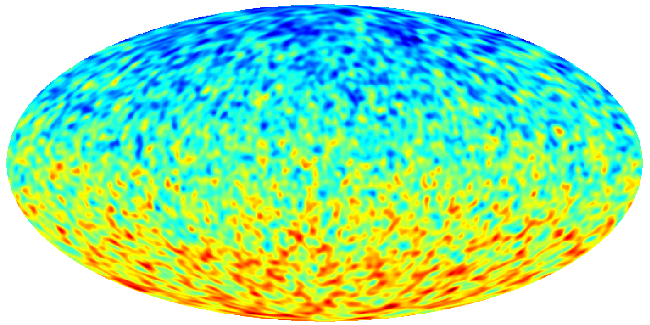
In order to demonstrate that the twelve scalar measures presented in section 2 are not all suited on the same footing to extract the modifications due to the aberration, two examples of them are given in figure 2, where the velocity $\beta=0.01$ is used. The panel 2(a) shows the aberrated temperature map obtained from the CMB rest frame by applying the velocity $\beta=0.01$ in the $z$-direction which corresponds to the north pole (“above”) in these sky maps. The aberration effect is almost invisible. This changes drastically by computing the sky map which shows the value of the first eigenvalue $\lambda_{1}$ of the Hessian matrix instead of the aberrated temperature as revealed by panel 2(b). One recognizes a significant dipole contribution although the CMB rest frame realization has none, since its quadrupole contribution is the first non-vanishing multipole. As an example from the group of distortion measures, the figure 2(c) displays the ellipticity $e$ defined in eq.(13), and there is no asymmetry between the Northern and the Southern hemisphere, which could reveal a non-vanishing peculiar velocity. It should be noted that in all three panels of figure 2, a Gaussian smoothing with a full width half-maximum (FWHM) of $3^{\circ}$ is applied after the scalar measures are calculated from the expansion coefficients $a^{\text{(obs)}}_{\ell m}$ of the unsmoothed temperature map with $\ell_{\text{max}}=3000$.

Since figure 2 has emphazised that the scalar measures of section 2 are very different in their discriminating power to extract the aberration effects, it is therefore natural to ask for the best-suited quantity. To that aim a set of 1000 CMB realizations is generated using the peculiar velocity $\beta_{\odot}=0.00123$ and $\ell_{\text{max}}=3000$. The boost is chosen in the $z$-direction and the twelve scalar measures are computed from these 1000 aberrated CMB simulations. In the next step, the dipole of each of the 1000 maps for each of the twelve scalar measures is extracted which allows the determination of the orientation of the dipole. The agreement or the deviation of this orientation from the boost orientation chosen in the simulations reveals the usability of the considered scalar measure. In spherical coordinates, the direction of the $z$-axis is given by the polar angle $\vartheta=0$ which thus defines the correct forward direction. The backward direction corresponds then to $\vartheta=\pi$, of course. A suitable scalar measure should thus yield a value close to $\vartheta=0$ for the forward direction and close to $\vartheta=\pi$ for the backward direction. The distributions of the orientations obtained in this way are shown in the histograms in figure 3. The bin width of histograms should be equal for the variable $x=\cos\vartheta$, so that each bin refers to the same size of the corresponding solid angle. Thus, the histograms discussed in the following cover the interval from $\cos\vartheta=-1$ to $\cos\vartheta=1$.

The normalized histograms in figure 3 show the probability distribution of $\cos\vartheta$ where the polar angle $\vartheta$ is determined from the orientation of the dipole $\ell=1$ of the corresponding twelve scalar measures. In order to compute this dipole orientation, all expansion coefficients $a_{\ell m}$ are set to zero except those three belonging to $\ell=1$ from which a sky map is generated whose maximal and minimal values yield the dipole orientation. Each panel in figure 3 displays two histograms, one reveals the angle $\vartheta$ obtained from the maximum of the dipole and the other from the minimum. As might be expected from figure 2, the eigenvalue $\lambda_{1}$ has a good discriminating power as revealed by the sharp peaks in the histogram at $\cos\vartheta=-1$ and $\cos\vartheta=1$. The same applies to the other eigenvalue $\lambda_{2}$ although the orientation of the dipole is swapped. The panel 3(c) presents the histogram of the Laplacian $\lambda_{+}$ given in eq. (9). Although the aberration direction is recognized in a lot of realizations, there are also many false detections as revealed by the non-vanishing bins even close to the equator. This distracting feature is absent for the determinant $d$ of the Hessian matrix, although the comparison of its histogram with those of the eigenvalues $\lambda_{1}$ and $\lambda_{2}$ uncovers a greater width and thus, a more unreliable detection of the boost direction. The histograms in figures 3(e) to 3(h) corresponds to the group of distortion measures. The histograms reveal a good discriminating power for the shear $y$ and for the distortion $\lambda_{-}$, while the ellipticity $e$ and the shape index $\iota$ are unusable as seen by the equidistributed histograms. The sky map corresponding to the ellipticity $e$ was already shown in figure 2(c), where also no boost signature was noticeable. The square of the gradient modulus $g$ is able to detect the boost direction as seen in figure 3(i), but it is more unreliable than the eigenvalues $\lambda_{1}$ or $\lambda_{2}$ as one observes from the width of the histograms. The derivative $D_{g}$ peaks also towards the peculiar velocity, but it is indifferent with respect to its direction as seen in figure 3(j). Finally, the last two panels reveal that the Gaussian curvature $\kappa_{\text{G}}$ as well as the extrinsic curvature $\kappa_{\text{ex}}$ are unsuitable due to the equidistributed histograms.

Since there are four scalar measures with a good detection characteristic as follows from the discussion of figure 3, it is more quantitative to consider the median of their distributions. The median values of the angular difference of direction of the dipole from the boost direction is listed in table 1. In the anti-boost direction, the listed value should be compared with $\vartheta=180^{\circ}$. One observes from table 1 that the best scalar measures are the two eigenvalues $\lambda_{1}$ and $\lambda_{2}$, the shear $y$ and the distortion $\lambda_{-}$. Although the square of the gradient modulus $g$ is more easily computed, since only first order derivatives are needed, its median is roughly twice as large as for the four best measures. These median values are computed by using the solar system velocity and, of course, would yield more accurate results for higher velocities.

The eigenvalues $\lambda_{1}$ and $\lambda_{2}$ determine not only the direction of the peculiar velocity but also its modulus. This is demonstrated in figure 4 where the maximal value $D_{\lambda_{1}}(\beta)$ of the dipole of $\lambda_{1}$ is plotted for several different values of the peculiar velocity $\beta$. One observes a linear behaviour such that the amplitude of the dipole can be used to estimate also the magnitude of the velocity. The linear behaviour is well approximated by the fit

with

and

where the coefficients are determined from the simulations based on the $\Lambda$CDM model specified above. The inset in figure 4 displays the distribution of the maximal values $D(\beta)$ for the 1000 simulations for the case $\beta_{\odot}=0.00123$ which possess a standard deviation of $\sigma=12699\mu\hbox{K}$ around the mean value $D_{\lambda_{1}}(\beta_{\odot})=94391\mu\hbox{K}$. The standard deviation $\sigma$ is of the same order for the other considered values of $\beta$. Since the fit value for $c_{0}$ is compatible with zero, the constant $c_{0}$ can be neglected. Thus, if the observations would determine $D_{\lambda_{1}}$ with sufficient accuracy, the modulus of velocity $\beta$ could be determined with an accuracy of the order $\sigma/c_{1}\simeq 1.6\times 10^{-4}$.

Up to now, the peculiar velocity is solely determined from the dipole orientation extracted from the corresponding scalar measure. Thus, one might wonder whether the inclusion of higher multipoles could increase the accuracy. To that aim, the extrema in the sky maps computed from the sum of the dipole and the quadrupole contribution are also investigated. Because one might also worry about the sharp cut-off at $\ell=2$ or $\ell=3$, respectively, a strong smoothing with Gaussian of FWHM of $45^{\circ}$ and of $90^{\circ}$ is additionally taken into account. The results are presented in figure 5 for the example of the first eigenvalue $\lambda_{1}$. The position of the minimum of the values of $\lambda_{1}$ on the sphere are determined, which should point approximately in the boost direction $\vartheta=0$. It is clearly seen that the sharpest distribution towards $\cos\vartheta=1$ is obtained by using only the dipole. Taking higher multipoles into account leads to a smearing of the distribution and thus to a more unreliable estimate for the boost direction.

In the case of partial sky observations, one has to deal with the difficulty to determine the dipole in the presence of a masked sky. The dipole then has to be fitted to the map of the eigenvalue $\lambda_{1}$ in the observed part of the sky. The full sky analysis of this work leads to the suggestion that the best estimate for our peculiar velocity will probably be achieved by fitting the dipole to the unsmoothed map. Without smoothing one does not need to care about smoothing a masked sky which is usually carried out in the $a_{\ell m}$ space by multiplying the expansion coefficients $a_{\ell m}$ with $F_{\ell}=\exp(-\frac{1}{2}\alpha^{2}\theta_{G}^{2}\,\ell(\ell+1))$ and $\alpha=\pi/(180\sqrt{8\ln 2})$ if the smoothing $\theta_{G}$ is given in degrees. This requires the determination of the coefficients $a_{\ell m}$ from a partial sky observation with a probably complicated mask structure. We thus suggest a three parameter fit, which is the dipole amplitude and the two angles for its orientation, to the unsmoothed map using a least-squares fitting, for example. This can be achieved by minimizing the expression

where $p^{i}_{\text{dip}}(\beta,\vartheta,\varphi)$ denotes the dipole value at pixel $i$ with the dipole orientation given by $\vartheta$ and $\varphi$. Furthermore, $p^{i}$ is the value of the $\lambda_{1}$ map at pixel $i$ and $\sigma_{i}$ the estimated error for this pixel. The sum runs only over the observed pixels. This procedure should also be favourable to reduce the uncorrelated pixel-to-pixel noise. It is clear that observations of too small a fraction of the sky will not allow a reliable determination of the peculiar velocity.

The motion of our solar system relative to the CMB rest frame leads to the large CMB dipole and to subtle distortions in the CMB sky map due to the aberration effect. Our peculiar velocity is usually derived from the dipole component of the CMB sky. It is then assumed that the CMB dipole is a pure Doppler dipole and a further intrinsic dipole and secondary effects can be safely ignored. It is thus desirable to have an independent method for the determination of the peculiar velocity. The aberration effect leads to mode couplings in the angular power spectrum which can betray the motion as discussed in the Introduction. However, if one tries to circumvent the determination of the spherical harmonic expansion coefficients $a_{\ell m}$, one can consider covariant derivatives on the sphere which measure the extent of the distortions being a compression of structures in the forward direction and a stretching in the backward direction. This method thus requires CMB maps with sufficiently high resolution. But since no full sky expansion is required as long as the process of derivation can be carried out with the observational data, high-resolution partial data would be suitable as provided by the Simons Observatory (Ade et al. 2019) and by CMB-S4 (Abazajian et al. 2019). The direct use of the partial derivatives on the sphere with respect to the coordinates $\vartheta$ and $\varphi$ has the disadvantage that they depend on the orientation of the spherical coordinate system. This is circumvented by the use of scalar measures, where in this work the twelve scalar quantities suggested by Monteserín et al. 2005 are investigated. The main result is that the eigenvalues $\lambda_{1}$ and $\lambda_{2}$ of the Hessian matrix defined in eqs.(7) and (8), the shear $y$ and the distortion $\lambda_{-}$ given in (11) and (12), respectively, are the best choices for detecting the boost direction. The remaining eight scalar quantities are not well-suited for this task. And it is demonstrated that the peculiar velocity is most accurately determined by extracting only the dipole contribution from the four favourable scalar measures.

The software packages HEALPix (http://healpix.jpl.nasa.gov, Górski et al. 2005) and CAMB written by A. Lewis and A. Challinor (http://camb.info/) as well as the Planck data from the LAMBDA website (http://lambda.gsfc.nasa.gov) were used in this work. Furthermore, we would like to thank the unknown referee for his useful comments.

The data underlying this article will be shared on reasonable request to the corresponding author.

References

- Abazajian et al. (2019) Abazajian K., et al., 2019, arXiv:1907.04473
- Ade et al. (2019) Ade P., et al., 2019, J. Cosmology Astropart. Phys., 2019, 056
- Amendola et al. (2011) Amendola L., Catena R., Masina I., Notari A., Quartin M., Quercellini C., 2011, J. Cosmology Astropart. Phys., 07, 027
- Burles & Rappaport (2006) Burles S., Rappaport S., 2006, ApJ, 641, L1
- Catena & Notari (2013) Catena R., Notari A., 2013, J. Cosmology Astropart. Phys., 04, 028
- Challinor & van Leeuwen (2002) Challinor A., van Leeuwen F., 2002, Phys. Rev. D, 65, 103001
- Chluba (2011) Chluba J., 2011, MNRAS, 415, 3227
- Dai & Chluba (2014) Dai L., Chluba J., 2014, Phys. Rev. D, 89, 123504
- Doré et al. (2003) Doré O., Colombi S., Bouchet F. R., 2003, MNRAS, 344, 905
- Górski et al. (2005) Górski K. M., Hivon E., Banday A. J., Wandelt B. D., Hansen F. K., Reinecke M., Bartelmann M., 2005, ApJ, 622, 759
- Jeong et al. (2014) Jeong D., Chluba J., Dai L., Kamionkowski M., Wang X., 2014, Phys. Rev. D, 89, 023003
- Kim & Naselsky (2010) Kim J., Naselsky P., 2010, ApJ, 714, L265
- Kogut et al. (1993) Kogut A., et al., 1993, ApJ, 419, 1
- Kosowsky & Kahniashvili (2011) Kosowsky A., Kahniashvili T., 2011, Phys. Rev. Lett., 106, 191301
- Land & Magueijo (2005) Land K., Magueijo J., 2005, Phys. Rev. D, 72, 101302
- Monteserín et al. (2005) Monteserín C., Barreiro R. B., Sanz J. L., Martínez-González E., 2005, MNRAS, 360, 9
- Mukherjee et al. (2014) Mukherjee S., De A., Souradeep T., 2014, Phys. Rev. D, 89, 083005
- Notari et al. (2014) Notari A., Quartin M., Catena R., 2014, J. Cosmology Astropart. Phys., 03, 019
- Planck Collaboration: Aghanim et al. (2014) Planck Collaboration: Aghanim N., et al., 2014, A&A, 571, A27
- Planck Collaboration: Aghanim et al. (2020) Planck Collaboration: Aghanim N., et al., 2020, A&A, 641, A1
- Planck Collaboration: Akrami et al. (2020) Planck Collaboration: Akrami Y., et al., 2020, A&A, 641, A7
- Yasini & Pierpaoli (2017) Yasini S., Pierpaoli E., 2017, Phys. Rev. D, 96, 103502
- Yasini & Pierpaoli (2020) Yasini S., Pierpaoli E., 2020, MNRAS, 493, 1708