Symmetry-protected multifold exceptional points and their topological characterization

Since the discovery of graphene, Dirac points have been revealed to be an ubiquitous property of various two dimensional (2D) materials. The existence of such 2-fold degeneracies is enforced by symmetries van Miert and Smith 2016; Young and Kane 2015, and their stability can be expressed with winding numbers of the phase of the wave functions Ando et al. 1998; Mikitik et al. 2008; Fuchs et al. 2010. Similarly, non-hermitian Hamiltonians may exhibit degeneracy points of their complex eigenvalues, called exceptional points (EPs). The quest for EPs, their topological properties and their physical implications, stimulated tremendous efforts in the past few years Bergholtz et al. 2019; Ashida et al. 2020; Shen et al. 2018; Zhou et al. 2018; Kozii and Fu 2017; Yoshida et al. 2018; Rausch et al. 2021; Yoshida et al. 2020; Hofmann et al. 2020; Shi et al. 2016. At an EP, the number of degenerated eigenvalues (the algebraic multiplicity $\mu$) is generically larger than the number of eigenvectors (the geometric multiplicity) leaving the Hamiltonian non-diagonalizable. Quite remarkably, 2-fold EPs (EP2s) do not require any symmetry to be stable in 2D, and this stability can be expressed in terms of a winding number Shen et al. 2018 associated to their complex eigenvalues Yang et al. 2019. This is however not the case for multi-fold exceptional points EP$\mu$s. Those were indeed shown to be unstable in 2D Yang et al. 2019, although stable in higher $D=2\mu-2$ dimension Höller et al. 2020; Bergholtz et al. 2019, so that EP$\mu$s beyond $\mu=2$ have remained overlooked. Still, a few examples of multifold EPs were surprisingly reported recently Xiao et al. 2020; Hatano 2019; Khandelwal et al. 2021, including in PT-symmetric systems Zhang et al. 2020. This asks the crucial question of the conditions of existence of multifold EPs, in particular in dimensions $D\leq 3$, their robustness and the role of symmetries.

Here we answer this question by showing that $\mu$-fold EPs have a codimension $\mu-1$ provided certain anti-unitary symmetries are satisfied, meaning that they appear as isolated points in $\mu-1$ dimensions. The relevant symmetries consist in PT symmetry, CP symmetry and their generalizations, called pseudo-Hermiticity (psH) and pseudo-chirality (psCh), that classify non-Hermitian EPs Kawabata et al. 2019; Yoshida et al. 2020. It follows that 3-fold and 4-fold EPs are stable in 2D and 3D respectively when such symmetries apply. Then, we propose a topological characterization for symmetry-protected EP$\mu$s through the homotopy properties of a resultant vector that we introduce. Finally, we illustrate our theory by discussing a frictional fluid model that exhibits several EP3s with opposite windings. These EPs constitute a threshold beyond which the propagation of all the eigenmodes vanishes in a certain range of wavelength, but can counter-intuitively be recovered when increasing friction furthermore.

To investigate $n$-fold EPs, we focus on $n\times n$ matrices without loss of generality, because $n$-fold degeneracies are described by a $n\times n$ effective Hamiltonians $H(\boldsymbol{\lambda})$, with $\boldsymbol{\lambda}\in\mathbb{R}^{D}$. The degeneracies of the eigenvalues $E(\boldsymbol{\lambda})$ are generically EPs, since arbitrary non-Hermitian matrices require fine tuning to be diagonalizable at the degeneracy point SM. Therefore, looking for $n$-fold EPs essentially amounts to searching for the conditions such that the characteristic polynomial $P_{\boldsymbol{\lambda}}(E)\equiv\det(H(\boldsymbol{\lambda})-E)=a_{n}(\boldsymbol{\lambda})E^{n}+a_{n-1}(\boldsymbol{\lambda})E^{n-1}+\dots+a_{1}(\boldsymbol{\lambda})E+a_{0}(\boldsymbol{\lambda})$ has $n$-fold multiple roots and $n=\mu$.

At an EP$\mu$ of energy $E_{0}$, $P_{\boldsymbol{\lambda}}(E)$ and its $\mu-1$ successive derivatives $P_{\boldsymbol{\lambda}}^{(j)}(E)\equiv\partial^{j}P_{\boldsymbol{\lambda}}/\partial E^{j}$ must vanish at $E=E_{0}$. This property is encoded in the zeros of the so-called resultant $R_{P,P^{(j)}}(\boldsymbol{\lambda})$. The resultant of two polynomials $P_{1}(E)$ and $P_{2}(E)$ is an elementary concept in algebra Gelfand et al. 1994. It reads $R_{P_{1},P_{2}}\equiv\det S_{P_{1},P_{2}}$ where $S_{P_{1},P_{2}}$ is the Sylvester matrix of $P_{1}$ and $P_{2}$. Importantly, this quantity vanishes if and only if the two polynomials $P_{1}$ and $P_{2}$ have a common root. Actually, we demonstrate (see SM) that a polynomial $P(E)$ of degree $\mu$ has an $\mu$-fold multiple root if and only if the resultants of its successive derivatives $R_{P^{(j-1)},P^{(j)}}$ vanish. Put formally,

$R_{P^{(j-1)},P^{(j)}}(\boldsymbol{\lambda})$ is in general a complex-valued function of $\boldsymbol{\lambda}$. The equivalence (Symmetry-protected multifold exceptional points and their topological characterization) thus yields $2(\mu-1)$ constraints to be satisfied, which gives the codimension of an EP$\mu$ in the absence of symmetry, in agreement with Höller et al. 2020; Bergholtz et al. 2019. Note that the usual EP2s are defined by $R_{P,P^{\prime}}(\boldsymbol{\lambda}_{0})=0$, where $R_{P,P^{\prime}}(\boldsymbol{\lambda})$ is proportional to the discriminant $\Delta$ of the characteristic polynomial. Since $\Delta$ is in general a complex function of $\boldsymbol{\lambda}$, the stability of EP2s can be expressed by the winding of $\arg(R_{P,P^{\prime}}(\boldsymbol{\lambda}))$ along a close circuit around $\boldsymbol{\lambda}_{0}$ in a 2D parameter space Yang et al. 2019.

As we discuss now, anti-unitary symmetries that are local in parameter space, have important consequences. First, they decrease the codimension of the EPs. Second, they make the discriminant $\Delta$ real. Thus sgn($\Delta$) becomes a well-defined quantity that one can use to characterize a spontaneous symmetry breaking. The winding of $\arg(\Delta)$ becomes ill-defined, but we shall see that another natural homotopy property can be assigned to multifold EPs.

The symmetries we consider are

where ^∗ stands for complex conjugation, ^† stands for Hermitian conjugation and the $U$’s are unitary operators. The consequences of these symmetries on the existence of EPs are readily obtained from the characteristic polynomial that must fulfill

Let us first proceed with PT-symmetry (5a). Then, the equation (6) implies $P_{\boldsymbol{\lambda}}(E)=a_{n}^{*}(\boldsymbol{\lambda})E^{n}+a_{n-1}^{*}(\boldsymbol{\lambda})E^{n-1}+\dots+a_{1}^{*}(\boldsymbol{\lambda})E+a_{0}(\boldsymbol{\lambda})^{*}$, so that $a_{l}^{*}(\boldsymbol{\lambda})=a_{l}(\boldsymbol{\lambda})$. All the coefficients $a_{l}(\boldsymbol{\lambda})$ must therefore be real. Thus, the resultants $R_{P^{(j-1)},P^{(j)}}(\boldsymbol{\lambda})$ are real too. This is due to the fact that the elements of the Sylvester matrix $S_{P^{(j-1)},P^{(j)}}$ are essentially the coefficients $a_{l}$ (multiplied adequately by numbers of the form $n(n-1)\cdots(n-j+1)$ due to the $j$ successive derivatives) Gelfand et al. 1994. The reality of the resultants implies that the number of conditions in (Symmetry-protected multifold exceptional points and their topological characterization) to have an EP$\mu$ reduces to $\mu-1$. By definition, the codimension of a PT-symmetry protected EP$\mu$ is therefore $\mu-1$.

Importantly, this codimension remains $\mu-1$ for any of the symmetries introduced in (5). This is obvious for pseudo-Hermiticity (5b), since taking the transpose of $H$ leaves invariant the determinant in Eq. (6). The case of CP-symmetry can be mapped onto the PT-symmetric one by the transformation $H\rightarrow-{\rm i}H$, that does not change the codimension of the degeneracies. Finally the pseudo-chiral case is deduced from the CP-symmetric one by invariance of Eq. (6) by taking the transpose of $H$. One can finally rephrase this result as : $\mu$-fold complex degeneracies of a $\mu\times\mu$ Hamiltonian satisfying one of the local anti-unitary symmetries (5) appear as ”defects” of dimension $d$ in a $D$-dimensional $\boldsymbol{\lambda}$-parameter space such that

Moreover, for each symmetry (5), the resultants $R_{P^{(j-1)},P^{(j)}}$ are real SM, consistently with the $\mu-1$ constraints (Symmetry-protected multifold exceptional points and their topological characterization) to be satisfied. The reality of the resultants naturally generates a resultant vector $\tilde{\boldsymbol{\mathcal{R}}}$ of components $R_{P^{(j-1)},P^{(j)}}$, that maps the $\boldsymbol{\lambda}$-space of parameters to $\mathbb{R}^{\mu-1}$. When the dimension of the $\boldsymbol{\lambda}$-space is $\mu-1$, the homotopy properties of the map $\boldsymbol{\lambda}\rightarrow\tilde{\boldsymbol{\mathcal{R}}}/|\tilde{\boldsymbol{\mathcal{R}}}|$ can be used to characterize the EP$\mu$.

In fact, a similar construction can be done from different resultants, so that another resultant vector, $\boldsymbol{\mathcal{R}}$, can be introduced. Indeed, the existence of an EP$\mu$ imposes resultants between other derivatives of $P(E)$ to vanish as well, and in particular

Actually, such a constraint, to be compared with (Symmetry-protected multifold exceptional points and their topological characterization), is also a necessary and sufficient condition for an EP$\mu$ to exist, at least for $\mu=2,3$ and $4$ SM. It turns out that those resultants are either real or purely imaginary. It is thus natural to define the resultant vector $\boldsymbol{\mathcal{R}}$ from its components

that depend on the symmetry, and where the coefficient $(-{\rm i})^{n(n-j)}$ guarantees the reality of $\mathcal{R}_{j}$.

The two resultant vectors we have introduced have the same first component $\mathcal{R}_{1}$, which is proportional to the discriminant $\Delta$ of the characteristic polynomial $P_{\boldsymbol{\lambda}}(E)$ of degree $n$ as $R_{P,P^{\prime}}(\boldsymbol{\lambda})=(-1)^{n(n-1)/2}a_{n}(\boldsymbol{\lambda})\,\Delta(\boldsymbol{\lambda})$. The vanishing of the discriminant at a given $\boldsymbol{\lambda}_{0}$ indicates the existence of at least two roots of $P_{\boldsymbol{\lambda}_{0}}(E)$. In the presence of a symmetry (5), the discriminant is also a real quantity, since both $R_{P,P^{\prime}}$ and $a_{n}$ are always real. Its sign (or equivalently that of $\mathcal{R}_{1}$) is therefore well defined and turns out to encode crucial properties about the complex eigenenergies $E_{j}$. For instance, it is well known that for a polynomial of degree $n=2$, $\Delta>0$ comes along with distinct real roots, while $\Delta<0$ indicates a pair of complex conjugated roots. These two behaviours are separated by a critical point $\Delta=0$ where the gap separating complex energy bands closes. More generally, a change in the number of complex conjugated roots is a property of the sign of the discriminant that generalizes beyond $n=2$ SM. One can thus use sign($\Delta$) as a $\mathbb{Z}_{2}$ index to distinguish two different regimes for non-Hermitian Hamiltonians of arbitrary size that satisfy one of the symmetries (5). The cases $n=2$ and $n=3$ are presented in table 1. Such an index encompasses the previously proposed topological invariants given by sgn$(\det H)$ [resp. sgn$(\det{\rm i}H)$] for $2\times 2$ PT [resp. CP] symmetric Hamiltonians Gong et al. 2018; Okugawa and Yokoyama 2019; Yoshida and Hatsugai 2019.

It is worth pointing out that a change of sign($\Delta$) reveals that the symmetry (5) under consideration is spontaneously broken. Let us recall this notion in PT-symmetric systems Bender and Boettcher 1998. Consider $H\ket{\psi}=E\ket{\psi}$, then $U_{PT}^{-1}\kappa\ket{\psi}$ is also an eigenstate of $H$ with eigenvalue $E^{*}$, where $\kappa$ is the complex conjugation operator. If $U_{PT}^{-1}\kappa\ket{\psi}$ is proportional to $\ket{\psi}$, then $\ket{\psi}$ is an eigenstate of the $PT$ operator, and the eigenenergies are real. In the other case, $\ket{\psi}$ is not an eigenstate of $U_{PT}^{-1}\kappa$ and the eigenenergies come by pairs $(E,E^{*})$. PT symmetry is then said to be spontaneously broken : it still holds at the level of the Hamiltonian, but not at the level of the eigenstates. The same reasoning applies to CP-symmetric and pseudo-chiral Hamiltonians, where eigenenergies come by either by pairs $(E,-E^{*})$ or are purely imaginary. In any case, the spontaneous symmetry breaking is accompanied with a change of sign of the discriminant that governs the complex nature and the pairing of the eigenvalues.

Symmetry-protected multifold EPs are special points where the symmetry is spontaneously broken, since they also demand the vanishing of the other components $\mathcal{R}_{j}=0$. From a geometrical point of view Yoshida et al. 2019; Yoshida and Hatsugai 2019; Kimura et al. 2019; Yoshida et al. 2020, the solutions $\boldsymbol{\lambda}$ of each equation $\mathcal{R}_{j}(\boldsymbol{\lambda})=0$ define a ”manifold” $\mathcal{M}_{j}$ of dimension $D-1$ in parameter space of dimension $D$ (i.e. codimension 1). Thus, the coordinates $\boldsymbol{\lambda}_{0}$ of EP$\mu$s define a space that consists in their mutual $\mu-1$ intersections. For instance, in $D=2$ dimensions, $\mathcal{M}_{1}$ and $\mathcal{M}_{2}$ consist in curves in a plane, and their mutual intersections are points that correspond to EP3s. Importantly, such intersections are generically robust to perturbations. Let us illustrate this point on a concrete model, the rotating shallow water model with friction.

The linearized rotating shallow water model describes waves propagating in a thin layer of fluid in rotation. It is currently used to describe atmospheric and oceanic waves over large distances where the Coriolis force, encoded into a parameter $f$, is relevant Vallis 2017. We consider a non-Hermitian version of this model that reads $H\Psi=E\Psi$ with

with $\delta u_{x}$ and $\delta u_{y}$ the small variations of the horizontal fluid velocity, $\delta h$ a small variation of the fluid’s thickness, $k_{x}$ and $k_{y}$ the in-plane wave numbers, $\gamma_{x}$ and $\gamma_{y}$ the Rayleigh friction terms, and $\gamma_{N}$ the Newtonian friction. The competition between the two friction terms plays for instance a crucial role in the phenomenon of super-rotation Warneford and Dellar 2017. Actually, this minimal model equivalently describes active fluids where the thickness field $h$ is formally replaced by a pressure field. Souslov et al. 2019 In that context, it was shown that the $\gamma$ terms can also be negative, thus allowing for gain James et al. 2018. We now show that the friction terms generate symmetry-protected EP3s.

Assuming isotropic friction $\gamma_{x}=\gamma_{y}\equiv\gamma_{R}$, the model remains rotational symmetric and can thus be simplified by fixing a direction (say $k_{y}=0$). Moreover, any choice of $\gamma_{R}$ can be reabsorbed in $\gamma_{N}$ up to a global shift of the spectrum, that does not affect the existence of degeneracies, as $H=\gamma_{R}\mathbb{I}+\tilde{H}$ with

where $\gamma\equiv\gamma_{N}-\gamma_{R}$. This matrix satisfies CP-symmetry (5c) with $U_{CP}=\text{diag}(1,1,-1)$, and one thus expects EP3s of codimension $2$, according to the relation (7). Since the parameter space has a dimension $D=3$, with $\boldsymbol{\lambda}=\{k_{x},f,\gamma\}$, the set of EP3s must consist in a manifold of codimension 2, that is a line. For this specific model, the equation of this line can be derived explicitly from $\mathcal{R}_{1}(\boldsymbol{\lambda}_{0})=0$ and $\mathcal{R}_{2}(\boldsymbol{\lambda}_{0})=0$, which yields $\gamma_{0}=\pm 3\sqrt{3}f_{0}$ and $k_{0}=\pm 2\sqrt{2}f_{0}$. Geometrically, this line of EP3s corresponds to the intersection of the two spaces $\mathcal{M}_{1}$ and $\mathcal{M}_{2}$, each of codimension 1. $\mathcal{M}_{1}$ and $\mathcal{M}_{2}$ are thus surfaces in 3D (figure 1 (a)), and lines in 2D (Fig. 1 (b) and (c)).

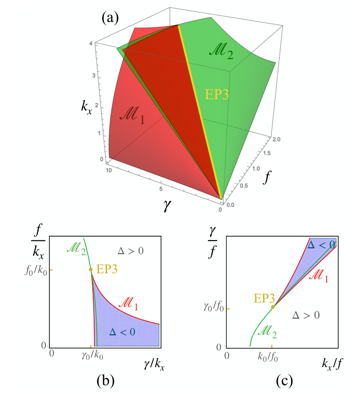
Remarkably, the space $\mathcal{M}_{1}\cap\mathcal{M}_{2}$ of EP3s correspond to a fold of $\mathcal{M}_{1}$. Similar singular points to that shown in figure 1 (b) and (c) were found in Xiao et al. 2020; Hatano 2019. This suggests a quite fundamental property of EP3s, that can be addressed within catastrophe theory which classifies the possible kinks of curves and thus establishes their topological stability Castrigiano and Hayes 2018. Intuitively, such a singular shape can be traced back to the third order characteristic polynomial $P_{\boldsymbol{\lambda}}(E)=0$, since cubic curves are known as a basic example that displays such a catastrophe when the three roots coincide. To characterize more precisely this singularity, we use the machinery of catastrophe theory and compute a list of invariants (called corank, codimension and determinacy) that classify the catastrophe. Following Castrigiano and Hayes 2018; Chandrasekaran et al. 2020, we find a corank of $1$, a codimension of $1$ and a determinacy of $3$, which identifies EP3s as a fold of $\mathcal{M}_{1}$. This is the simplest fundamental catastrophe in the classification of catastrophe theory.

Before characterizing in more details the robustness of the EP3, let us first comment on the original physical behaviours revealed in figure 1. Indeed, $\mathcal{M}_{1}$ indicates a change of sign of the discriminant, and thus, according to table 1, it denotes a transition between complex eigenvalues ($\Delta>0$) and purely imaginary eigenvalues $(\Delta<0)$, which, in our case, all have the same sign which is fixed by sgn$(\gamma)$. The eigenvalue spectrum of (12) is shown in figure 2. It follows that the $\Delta<0$ domain corresponds to a regime where all the eigenmodes are fully evanescent (for $\gamma>0$) and thus where propagation is prohibited. Quite remarkably, while a first propagating $\rightarrow$ non-propagating transition happens when increasing friction, an even more striking non-propagating $\rightarrow$ propagating second transition occurs when increasing dissipation furthermore. In those phase diagrams, the EP3 appears as the threshold beyond which such transitions exist.

One can characterize the stability of symmetry protected EPs furthermore by using the topological properties of the resultant vector $\boldsymbol{\mathcal{R}}\in\mathbb{R}^{\mu-1}$ introduced above. For an EP3, it defines a map $\boldsymbol{\mathcal{R}}/|\boldsymbol{\mathcal{R}}|\mathrel{\mathop{\mathchar 58\relax}}\mathbb{R}^{2}\backslash\{\boldsymbol{\lambda}_{0}\}\rightarrow S^{1}$ whose homotopy properties are encoded into the integer-valued winding number

where the close circuit $\mathcal{C}_{\boldsymbol{\lambda}}$ surrounds the EP3 and where an implicit sum is taken over $\alpha=\{1,2\}$. It is worth noticing that, in lattice systems, $\mathcal{M}_{1}$ and $\mathcal{M}_{2}$ are necessarily closed loops in the 2D Brillouin zone, so that their intersections come by pairs with opposite $W_{3}$’s, which can be seen by a straightforward extension of the doubling theorem by Nielsen and Ninomiya Nielsen and Ninomiya 1981a; Nielsen and Ninomiya 1981b as recently generalized for non-Hermitian systems without symmetry Yang et al. 2019.

The invariant $W_{3}$ is the winding number of the relative angle between $\mathcal{R}_{1}$ and $\mathcal{R}_{2}$. For the frictional shallow water model, its value is shown in figure 3 (a). It turns out that in this model, EP3s come by pairs $W_{3}=\pm 1$ at $k_{x}=\pm k_{0}$. This indicates that such pairs may possibly merge and annihilate each other if one moves them, similarly to Dirac and Weyl points in semimetals Dietl et al. 2008; Wunsch et al. 2008; Montambaux et al. 2009; Delplace et al. 2012. Since the position of the EP3s is fixed in the isotropic case, a mechanism involving their motion necessarily breaks rotational symmetry. This can be achieved by considering now $\gamma_{x}\neq\gamma_{y}$, as shown in figure 3 (a) where one pair ($\gamma_{N}/f>0$) get closer while the other pair ($\gamma_{N}/f<0$) is pulled away. When increasing $\gamma_{x}$ furthermore, the points of the pair at $\gamma_{N}/f>0$ finally merge. Surprisingly enough, a new domain of non-propagating waves ($\Delta<0$) emerges for $\gamma_{N}<0$ (see Fig. 3 (b)).A similar analysis can be carried out from the other resultant vector $\tilde{\boldsymbol{\mathcal{R}}}$ introduced above, but its winding number is found to be zero for that model.

More generally, multifold ($\mu\geqslant 3$) symmetry-protected EPs can be characterized by the homotopy properties of their resultant vectors $\boldsymbol{\mathcal{R}}$ (or $\tilde{\boldsymbol{\mathcal{R}}}$). Let us fix $d=0$, so that the EP is an isolated point $\boldsymbol{\lambda}_{0}\in\mathbb{R}^{\mu-1}$, according to (7). Then the resultant vector defines the map $\boldsymbol{\mathcal{R}}/|\boldsymbol{\mathcal{R}}|\mathrel{\mathop{\mathchar 58\relax}}\mathbb{R}^{\mu-1}\backslash\{\boldsymbol{\lambda}_{0}\}\rightarrow S^{\mu-2}$ whose degree¹¹ 1 Not to be confused with the degree of the characteristic polynomial. $W_{\mu}\equiv\deg\boldsymbol{\mathcal{R}}\in\mathbb{Z}$ is well-defined and reads Dubrovin et al. 1985

where $\boldsymbol{\mathcal{R}}_{0}$ is an arbitrary point where the Jacobian matrix $(\partial\mathcal{R}_{j}/\partial\lambda_{p})$ does not vanish. This homotopy invariant is a topological property of multifold symmetry-protected EPs. The expression (13) of the winding number $W_{3}$ for EP3s is the simplest example of such invariants.

Our analysis opens various novel perspectives in the control of topological properties of non-Hermitian systems. In future works, it could be interesting to investigate symmetry-protected EP4s that should appear in three-dimensional parameter spaces, and whose topological charge $W_{4}$ takes the form of a wrapping number of the resultant vector

In particular, this suggests the existence of stable non-Hermitian versions of 3D Dirac points in sharp contrast with both Hermitian 3D Dirac points and non-Hermitian Weyl points that were both found to be unstable.