Research on causal inference to examine the magnitude of the effect of the treatment variable on the outcome variable is one of the important tasks in data science. Fisher’s randomized controlled trial is one of the most important methods to examine the causal effect and is often considered as the gold standard for causal inference [Fisher, 1951]. However, complete randomization is often impracticable due to cost or ethical reasons, demanding methods for identifying causal effects for non-experimental observational studies.

To identify causal effects in observational studies, it is necessary to make some assumptions on the data generating process. There are various interrelated approaches to statistically estimate causal effects, including those based on propensity scores [Guo and Fraser, 2014], those based on instrumental variables [Angrist et al., 1996], and those based on Structural Causal Model (SCM) [Pearl, 2000]. In this study, we focus on the causality estimation based on SCM. In SCM, we are interested in examining the causal effect of a treatment variable $X$ on an outcome variable $Y$, which is written as an experimental distribution $p(y|\mbox{do}(X=x))$, where $\mbox{do}(X=x)$ means that $X$ is fixed to $x$ by an intervention. The causal effect $p(y|\mbox{do}(X=x))$ is calculated based on the knowledge on a causal graph $G$, which describes a coarse relationship among the observable variables, and a distribution $P(X,Y,Z_{1},\ldots,Z_{c})$, where $Z_{1},\ldots,Z_{c}$ are observable variables (covariates) other than $X$ and $Y$.

In general, we do not know the true causal graph $G$, so there are various methods for estimating the causal graph from the data [Spirtes and Glymour, 1991, Cooper and Herskovits, 1992, Heckerman et al., 1995, Shimizu et al., 2006]. Furthermore, to calculate the causal effect, it has to estimate the conditional distributions among the variables. Therefore, a general way to estimate the causal effect consits of the following steps.

1. 1.

   Estimate the causal graph from the data

2. 2.

   Estimate the conditional distributions among the variables from the data

3. 3.

   Calculate the causal effect

However, if the goal is to estimate the causal effect, it is not necessary to fix a single causal graph or distributions. We first derive the Bayesian optimal estimator when the problem is to estimate the mean causal effect under the squared error loss. The Bayes optimal solution turns out to be the estimator that weights the mean causal effects estimated under each model, which is also known as Bayesian model averaging [Hoeting et al., 1999]. In the literature of causal inference, Bayesian model averaging is applied for propensity score analysis [Kaplan and Chen, 2014], however, our study is an attempt to apply it for the causal inference based on SCM. The basic idea behind our proposal is to consider the causal graph and the parameters of the distributions as parameters to be marginalized in estimating the causal effect. Although the model setting is different, a similar idea can be found in [Rubin, 1978], where the values of the unobserved potential outcomes are treated as parameters to be marginalized.

Although the Bayesian model averaging is optimal, as the number of candidate models increases, the weighting calculations become computationally hard. In this paper, we develop an approximation algorithm for the case where the following assumptions hold.

1. 1.

   We know the set of possible directed edges, including information on the directions of the edges.

2. 2.

   We do not know whether each element of the above set of possible directed edges exists. We only know the prior probability that each directed edge exists.

The above assumptions make sense in some practical applications. For example, consider the case where there are $m$ variables $X_{1},\ldots,X_{m}$ and only the antecedent relations, such as nodes with higher index numbers do not precede nodes with lower index numbers, to the causal relations among these variables are known. This is the situation dealt with in [Wermuth and Lauritzen, 1982]. In this case, the set of possible directed edges are given by $\left\{(i,j):i<j,1\leq i,j\leq m\right\}$.

Even if we put the constraint above, the number of models grows exponentially with the number of possible directed edges. We develop an approximation to the Bayes optimal estimator by using sparse modeling techniques. The basic idea is to approximate a mixture distribution of Dirac delta function and Gaussian distribution with Gaussian scale mixture (GSM). In the prediction task, it is reported that performance similar to Bayesian model averaging can be achieved by using horseshoe prior, which is a kind of GSM [Carvalho et al., 2009]. This study shows that a similar approach is also effective in estimating causal effects.

The paper is organized as follows. In Section 2, some preliminary materials about SCM and corresponding causality notions such as the intervention effect and the mean intervention effect are described. In Section 3, we formulate the problem to estimate the mean intervention effect as a statistical decision problem and derive the optimal decision function under the Bayes criterion. Section 4 describes the further assumptions for the causal graph in this study and derives an approximation algorithm for the Bayes optimal decision function under these assumptions. Section 5 presents some experimental results to evaluate our proposals. Finally, we give a summary in Section 6.

As mentioned in the introduction, there are some approaches to statistically estimate causal effects. Since this study follows the framework of SCM, we borrow some basic notions of SCM.

One may think that the parametric assumption among the variables is too strong, however, a theory built on a simple model will be the foundations for a theory in more complex models, and as we will show in later experiments, even such a simple model works for some real-world problems.

Structural equations and causal graphs express coarse causal relationships among the variables. Given these information, we want to know the causal effect of a treatment variable $X\in V$ on an outcome variable $Y\in V$ when $X$ is fixed to a value $x$ by an external intervention. It is mathematically defined as follows [Pearl, 2000].

The intervention effect $p(y|{\rm do}(X=x))$ is defined as an experimental distribution. In this study, we focus on the estimation of their mean (expectation), the Mean Intervention Effect (MIE). The MIE $\bar{y}_{x}$ is defined as

When the model is linear SCM, it is known that the MIE is expressed as

where $\mathcal{P}$ is the set of the directed paths from $X$ to $Y$ [Pearl, 2000]. This is an equivalent notion of the total effect in [Wright, 1921].

We note that the main interest of the existing studies in the literature is the identifiability of the total effect. For example, Pearl proved a valuable result that claims that we can identify the total effect if we can observe some covariates that satisfy the backdoor criterion [Pearl, 2000]. On the other hand, our focus is how to estimate the total effect. Although it would be interesting to combine our results with the existing results, we do not use those results in this paper.

In order to calculate the MIE (5), one has to know the underlying causal graph $G$ and conditional distributions $p(x_{i}|{\rm pa}(x_{i})),i=1,\ldots,m$. Therefore, the data analyst must either proceed with the belief that the assumed causal graph is correct, or estimate the causal graph from the data. Although there are various methods for estimating the causal graph from the data [Spirtes and Glymour, 1991, Cooper and Herskovits, 1992, Heckerman et al., 1995, Shimizu et al., 2006], there is a possibility that these methods output a wrong causal graph. Furthermore, previous studies are rarely concerned about how to estimate the probability distributions $p(x_{i}|{\rm pa}(x_{i})),i=1,\ldots,m$ because their main concern is about the identifiability of the causal effects given the causal graph and probability distributions. However, it is uncommon to assume that the probability distribution is known without knowing the data generating causal graph. In our setting, we need to deal with the estimation of the probability distributions as well as the estimation of the causal graph.

We assume that the causal diagram $G$ is a random variable that takes its value in the set of DAGs $\mathcal{G}$ and whose prior distribution is $p(G)$. This prior distribution represents, for example, the data analyst’s confidence in each causal graph. Since we deal with the linear SCM, given a causal graph $G$, conditional distributions $p(x_{i}|{\rm pa}(x_{i}))$ are parameterized by $\theta_{ij},(i,j)\in E_{G}$ as follows.

Throughout the paper, we assume that the precision parameter $s_{\epsilon}$ of error is known. We can extend our results to the unknown case by assuming a prior distribution for $s_{\epsilon}$. Let $\bm{\theta}_{G}=\left(\theta_{ij}:(i,j)\in E_{G}\right)$. We assume that the parameter $\bm{\theta}_{G}$ is also a random vector whose conditional distribution under $G$ is $p(\bm{\theta}_{G}|G)$. Since the MIE is the function of $G$ and $\bm{\theta}_{G}$, we write it as $\bar{y}_{x}(G,\bm{\theta}_{G})$.

Let $D^{N}=\left(x_{n},y_{n},z_{1,n},\ldots,z_{c,n}\right)_{n=1,\ldots,N}$ be a sample of $V=(X,Y,Z_{1},\ldots,Z_{c})$ with sample size $N$. ²² 2 We sometimes do not distinguish $X$ and $Y$ from other covariates $Z_{1},\ldots,Z_{c}$. In that case, we write the set of variables as $V=(X_{1},X_{2},\ldots,X_{m})$. We consider the problem of estimating the MIE (5) given $D^{N}$. Let $d:D^{N}\mapsto\mathbb{R}$ be a decision function that outputs an estimate of the MIE. The loss function is the metric between the estimand and the decision function. In this study, the squared error loss is used, i.e.,

In the statistical decision theory framework [Berger, 2013], the risk function and the Bayes risk function are defined as follows, respectively.

The Bayes optimal estimator, that minimizes the Bayes risk function, is given as follows.

Note that the Bayes optimal estimator of the intervention effect under the Kullback-Leibler loss is given in [Horii and Suko, 2019].

In general, numerical integration is required to calculate the integrals in (10) since $\bar{y}_{x}(G,\bm{\theta}_{G})$ is a nonlinear function of $\bm{\theta}_{G}$. When the computational complexity of the numerical integration is large, we approximate (10) by

This approximation is based on the property that the posterior distribution $p(\bm{\theta}_{G}|G,D^{N})$ is asymptotically concentrated around $\bm{\theta}_{G}^{MAP}$ under some appropriate conditions [Le Cam, 2012]. To keep the description concise, we call the estimator (15) Bayes quasi-optimal estimator.

If the prior distribution $p(\bm{\theta}_{G}|G)$ is a product of Gaussian, namely,

we can analytically calculate $p(G|D^{N})$ and $p(\bm{\theta}_{G}|G,D^{N})$. See the supplementary material for the derivation.

The problem with calculating (10) or (15) in practical applications is that its computational complexity is proportional to the number of candidate models. The number of possible DAGs for a given set of variables $V=(X_{1},X_{2},\ldots,X_{m})$ is $O\left(2^{m^{2}}\right)$. However, it would be uncommon to know nothing at all about the structure of a graph, and we might know the causal relationships among some variables and not the rest. Therefore, in this study, we classify the directed edges expressing the causal relationships among variables into three types.

• •

  It is known that there is a causal relationship between variables, including information on which is the cause and which is the result. In other words, there is a directed edge between the corresponding variables with probability 1.

• •

  It is known that there is no causal relationship between the corresponding variables. In other words, there is directed edge between the corresponding variables with probability 0.

• •

  If there is a causal relationship, it is known that which is the cause and which is the result, but it is not clear whether the causal relationship exists. In other words, there is a directed edge between the corresponding variables with some probability.

For the sake of simplicity, we assume that the set of the edges of the first type is empty, since they can be considered as the edges of the third type with edge existence probability set to 1.

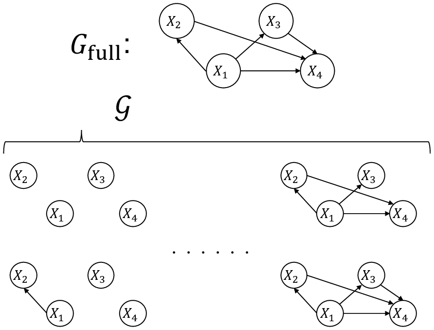
Let $E_{\rm full}$ be a set of possible directed edges connecting nodes that may or may not have a causal relationship between the corresponding variables. We assume that $(j,i)\notin E_{\rm full}$ if $(i,j)\in E_{\rm full}$. The set $\mathcal{G}$ of the candidate causal graphs is defined as

Let $G_{\rm full}$ be the abbreviation for $G_{E_{\rm full}}$. Figure 1 depicts an example of $G_{\rm full}$ and $\mathcal{G}$.

We assume that there is a causal relationship between $X_{i}$ and $X_{j}$ for $(i,j)\in E_{\rm full}$ with probability $p$, that is, a directed edge $(i,j)$ exists with probability $p$. Then, the prior distribution $p(G)$ is given by

Even if the set of candidate models is restricted to (18), the number of candidate models $|\mathcal{G}|$ is $2^{|E_{\rm full}|}$, and when $|E_{\rm full}|$ is large, the calculation of (10) becomes infeasible.

For $G_{\rm full}$, consider the following experimental prior distribution.

where $\delta_{0}(\cdot)$ is the Dirac delta function. Such priors are often called spike-and-slab priors [Ishwaran et al., 2005]. Then, the following proposition holds.

When (20) and (21) are assumed, the Bayes optimal estimator can be rewritten as

where

With the introduction of the spike-and-slab prior, the problem of calculating the summation over the candidate models has apparently disappeared, but the calculation of (24) is still difficult because the calculation of the posterior distribution (25) is difficult.

We approximate $p_{ss}(\theta_{ij})$ by Gaussian scale mixture (GSM) [Andrews and Mallows, 1974, Boris Choy and Chan, 2008]. The probability density function (pdf) of GSM is given by

where $\bm{\alpha}$ is the parameter of the distribution $p(\bm{\tau};\bm{\alpha})$. Note that the values of $\tau_{ij}$ are different for different $(i,j)\in E_{\rm full}$. If $\tau_{ij}$ is small, it means that the probability that $\theta_{ij}$ takes a value close to 0 is large, and we want to estimate them from the data. The distribution $p(\tau_{ij};\bm{\alpha})$ is a distribution of the variance of Gaussian and it is often called mixing distribution. It is known that GSM can express various distributions, such as Laplace distribution, Student-t distribution and horseshoe distribution, by changing the mixing distribution. GSM is often used in the Bayesian sparse modeling literature. See [Ji et al., 2008], for example.

Even if we use GSM for the prior distribution $p(\theta_{ij})$, it is still difficult to calculate the exact posterior, however, there are various approximation algorithms to efficiently calculate the approximate posterior which are based on Expectation-Maximization (EM) algorithm [Figueiredo, 2003], Markov-Chain Monte-Carlo (MCMC) algorithm [Park and Casella, 2008], and Variational Bayes (VB) algorithm [Babacan et al., 2014]. As an example, we give an estimation algorithm based on the variational Bayes algorithm. See the supplementary material for the derivation of the algorithm.

Let $\bm{\theta}_{j}=\left(\theta_{ij}:(i,j)\in E_{\rm full}\right)$ and we describe an estimation algorithm for $\bm{\theta}_{j}$ since we can estimate $\bm{\theta}_{1},\ldots,\bm{\theta}_{m}$ independently. We use the exponential distribution as the mixing distribution, that is,

We have to determine or estimate the values of $\alpha_{ij}$. We take a Bayesian hierarchical modeling approach, that is, we further assume gamma distribution for $\alpha_{ij}$ which is the conjugate distribution of the exponential distribution.

where $\Gamma(\cdot)$ is the gamma function and $\kappa,\nu$ are hyper-parameters. By setting $\kappa,\nu$ so that $p(\alpha_{ij};\kappa,\nu)$ is flat, the algorithm can estimate $\alpha_{ij}$ as well as other parameters. The update equations for the variational Bayes algorithm are summarized as follows.

• •

  Update equation for $\bm{\theta}_{j}$

  	$\displaystyle\bar{\bm{\theta}}^{(t+1)}_{j}$	$\displaystyle=s_{\epsilon}\bm{\Sigma}^{(t+1)}_{j}\bm{X}_{j}^{T}\bm{x}_{j},$		(30)
  	$\displaystyle\bm{\Sigma}_{j}^{(t+1)}$	$\displaystyle=\left(s_{\epsilon}\bm{X}_{j}^{T}\bm{X}_{j}+\bar{\bm{S}}_{j}^{(t)}\right)^{-1},$		(31)

  where

  $\displaystyle\bar{\bm{S}}_{j}^{(t)}={\rm diag}\left(\bar{s}^{(t)}_{j,1},\ldots,\bar{s}^{(t)}_{j,m_{j}}\right),$

  (32)

  and ${\rm diag}(\bm{a})$ is the diagonal matrix whose diagonal elements are $\bm{a}$.

• •

  Update equation for $\left\{\tau_{j,i}\right\}$

  	$\displaystyle\bar{\tau}_{j,i}^{(t+1)}$	$\displaystyle=\frac{1+\sqrt{\bar{\alpha}_{j,i}^{(t)}\left((\bar{\theta}_{j,i}^{(t+1)})^{2}+\Sigma_{j,ii}^{(t+1)}\right)}}{\bar{\alpha}_{j,i}^{(t)}},$		(33)
  	$\displaystyle\bar{s}_{j,i}^{(t+1)}$	$\displaystyle=\sqrt{\frac{\bar{\alpha}_{j,i}^{(t)}}{(\bar{\theta}_{j,i}^{(t+1)})^{2}+\Sigma_{j,ii}^{(t+1)}}},$		(34)

  where $\bar{\theta}_{j,i}^{(t)}$ and $\Sigma_{j,ii}^{(t+1)}$ are the $i$-th element of $\bar{\bm{\theta}}_{j}^{(t)}$ and $(i,i)$-element of $\bm{\Sigma}_{j}^{(t+1)}$, respectively³³ 3 To make the description concise, indices of the variables are replaced so that $\theta_{j,i}=\theta_{j_{i}j}$..

• •

  Update equation for $\left\{\alpha_{j,i}\right\}$

  $\displaystyle\bar{\alpha}_{j,i}^{(t+1)}=(\kappa+1)\left(\nu+\frac{\bar{\tau}_{j,i}^{(t+1)}}{2}\right).$

  (35)

Starting from some initial values $\left\{\bar{s}_{j,i}^{(0)}\right\},\left\{\bar{\alpha}_{j,i}^{(0)}\right\}$ and iterating the above algorithm until it converges, we obtain an approximation posterior distribution $q(\bm{\theta}_{j}|D^{N})=\mathcal{N}(\hat{\bm{\theta}}_{j},\hat{\bm{\Sigma}}_{j}),j=1,\ldots,m$, where $\hat{\bm{\theta}}_{j}$ and $\hat{\bm{\Sigma}}_{j}$ are the convergence values of $\bar{\bm{\theta}}_{j}^{(t)}$ and $\bm{\Sigma}_{j}^{(t)}$, respectively. Using these, (24) and (15) are approximated as

respectively.

The computational complexity of an iteration of the algorithm is $O(m_{j}^{3})$, which comes from the inversion of the $m_{j}\times m_{j}$ matrix. If the dimension of the problem is too high to explicitly calculate $\bm{\Sigma}_{j}^{(t+1)}$, we have to use an approximate matrix inversion algorithm with low complexity. In this paper, we do not deal with such high-dimensional problems.

We proposed a Bayes optimal estimator of the MIE which minimizes the squared error loss on average when the data generating model is an unknown random variable. The proposed estimator has to estimate the causal effects under the all candidate causal graphs and it is hard to compute when the number of candidate causal graphs is large. We also proposed an approximation algorithm for the optimal estimator by using a sparse modeling technique. Some numerical experiments corroborated the effectiveness of our proposed methods. The proposed methods can help analysts when there is some ambiguity in the knowledge of the data generating model.

We have made some strong assumptions in this study:

• •

  Gaussian assumption on the prior or the error terms

• •

  Assumption that there is no hidden confounders

• •

  Assumption that causal orders are known

• •

  Linear assumption on the SCM

These assumptions might limit the range of the real-world applications of the proposed methods. We think that we can relax some assumptions by combining the proposed methods with previously known results. For example, if we can assume non-Gaussian distributions on the error terms, we can relax the assumption on causal orders since models with opposite causal directions would have different posterior probabilities. In such cases, the method proposed in this paper needs to be modified, and the constrution of such an algorithm would be an attractive research direction.

This research is partially supported by Information Services International-Dentsu (ISID), Ltd. Research Grant, the Kayamori Foundation of Informational Science Advancement, and No. 19K12128 of Grant-in-Aid for Scientific Research Category (C) and No. 18H03642 of Grant-in Aid for Scientific Research Category (A), Japan Society for the Promotion of Science.

References

- [Andrews and Mallows, 1974] Andrews, D. F. and Mallows, C. L. (1974). Scale mixtures of normal distributions. Journal of the Royal Statistical Society: Series B (Methodological), 36(1):99–102.
- [Angrist et al., 1996] Angrist, J. D., Imbens, G. W., and Rubin, D. B. (1996). Identification of causal effects using instrumental variables. Journal of the American statistical Association, 91(434):444–455.
- [Babacan et al., 2014] Babacan, S. D., Nakajima, S., and Do, M. N. (2014). Bayesian group-sparse modeling and variational inference. IEEE transactions on signal processing, 62(11):2906–2921.
- [Berger, 2013] Berger, J. O. (2013). Statistical decision theory and Bayesian analysis. Springer Science & Business Media.
- [Bishop, 2006] Bishop, C. M. (2006). Pattern recognition and machine learning. springer.
- [Boris Choy and Chan, 2008] Boris Choy, S. and Chan, J. S. (2008). Scale mixtures distributions in statistical modelling. Australian & New Zealand Journal of Statistics, 50(2):135–146.
- [Carvalho et al., 2009] Carvalho, C. M., Polson, N. G., and Scott, J. G. (2009). Handling sparsity via the horseshoe. In Artificial Intelligence and Statistics, pages 73–80.
- [Cooper and Herskovits, 1992] Cooper, G. F. and Herskovits, E. (1992). A bayesian method for the induction of probabilistic networks from data. Machine learning, 9(4):309–347.
- [Figueiredo, 2003] Figueiredo, M. A. (2003). Adaptive sparseness for supervised learning. IEEE transactions on pattern analysis and machine intelligence, 25(9):1150–1159.
- [Fisher, 1951] Fisher, R. A. (1951). The design of experiments.
- [Guo and Fraser, 2014] Guo, S. and Fraser, M. W. (2014). Propensity score analysis: Statistical methods and applications, volume 11. SAGE publications.
- [Heckerman et al., 1995] Heckerman, D., Geiger, D., and Chickering, D. M. (1995). Learning bayesian networks: The combination of knowledge and statistical data. Machine learning, 20(3):197–243.
- [Hill, 2011] Hill, J. L. (2011). Bayesian nonparametric modeling for causal inference. Journal of Computational and Graphical Statistics, 20(1):217–240.
- [Hoeting et al., 1999] Hoeting, J. A., Madigan, D., Raftery, A. E., and Volinsky, C. T. (1999). Bayesian model averaging: a tutorial. Statistical science, pages 382–401.
- [Horii and Suko, 2019] Horii, S. and Suko, T. (2019). A note on the estimation method of intervention effects based on statistical decision theory. In 2019 53rd Annual Conference on Information Sciences and Systems (CISS), pages 1–6. IEEE.
- [Horvitz and Thompson, 1952] Horvitz, D. G. and Thompson, D. J. (1952). A generalization of sampling without replacement from a finite universe. Journal of the American statistical Association, 47(260):663–685.
- [Ishwaran et al., 2005] Ishwaran, H., Rao, J. S., et al. (2005). Spike and slab variable selection: frequentist and bayesian strategies. The Annals of Statistics, 33(2):730–773.
- [Ji et al., 2008] Ji, S., Xue, Y., and Carin, L. (2008). Bayesian compressive sensing. IEEE Transactions on signal processing, 56(6):2346–2356.
- [Kaplan and Chen, 2014] Kaplan, D. and Chen, J. (2014). Bayesian model averaging for propensity score analysis. Multivariate behavioral research, 49(6):505–517.
- [Le Cam, 2012] Le Cam, L. (2012). Asymptotic methods in statistical decision theory. Springer Science & Business Media.
- [Park and Casella, 2008] Park, T. and Casella, G. (2008). The bayesian lasso. Journal of the American Statistical Association, 103(482):681–686.
- [Pearl, 2000] Pearl, J. (2000). Causality: Models, reasoning, and inference.
- [Rubin, 1978] Rubin, D. B. (1978). Bayesian inference for causal effects: The role of randomization. The Annals of statistics, pages 34–58.
- [Shimizu et al., 2006] Shimizu, S., Hoyer, P. O., Hyvärinen, A., and Kerminen, A. (2006). A linear non-gaussian acyclic model for causal discovery. Journal of Machine Learning Research, 7(Oct):2003–2030.
- [Shimoni et al., 2018] Shimoni, Y., Yanover, C., Karavani, E., and Goldschmnidt, Y. (2018). Benchmarking framework for performance-evaluation of causal inference analysis. arXiv preprint arXiv:1802.05046.
- [Spirtes and Glymour, 1991] Spirtes, P. and Glymour, C. (1991). An algorithm for fast recovery of sparse causal graphs. Social science computer review, 9(1):62–72.
- [Wermuth and Lauritzen, 1982] Wermuth, N. and Lauritzen, S. L. (1982). Graphical and recursive models for contigency tables. Institut for Elektroniske Systemer, Aalborg Universitetscenter.
- [Wright, 1921] Wright, S. (1921). Correlation and causation. J. agric. Res., 20:557–580.
Appendix A Derivation of the analytical form of and
First, we derive for a fixed . For , let and , where is the sample of . Then, for , the likelihood function is given by