跳到论文正文
W Papers独立论文阅读器 arXiv:2103.08041 论文正文 计算阅读时间 · 0%
引用这篇论文根据当前论文元数据生成,正式投稿前建议核对。


License: arXiv.org perpetual non-exclusive license
arXiv:2103.08041v2 [eess.SY] 04 Jun 2021

Safe Controller Synthesis with Tunable
Input-to-State Safe Control Barrier Functions

Anil Alan Affiliation: A. Alan, C. R. He, and G. Orosz are with the Department of Mechanical Engineering, University of Michigan, Ann Arbor, MI 48109, USA {𝚊𝚗𝚒𝚕𝚊𝚕𝚊𝚗,𝚑𝚌𝚑𝚊𝚘𝚣𝚑𝚎,𝚘𝚛𝚘𝚜𝚣}​@​𝚞𝚖𝚒𝚌𝚑.𝚎𝚍𝚞{\tt\small\{anilalan,hchaozhe,orosz\}@umich.edu}    Andrew J. Taylor Affiliation: A. J. Taylor and A. D. Ames are with the Department of Mechanical and Civil Engineering, California Institute of Technology, Pasadena, CA 91125, USA {𝚊𝚓𝚝𝚊𝚢𝚕𝚘𝚛,𝚊𝚖𝚎𝚜}​@​𝚌𝚊𝚕𝚝𝚎𝚌𝚑.𝚎𝚍𝚞{\tt\small\{ajtaylor,ames\}@caltech.edu}    Chaozhe R. He Affiliation: A. Alan, C. R. He, and G. Orosz are with the Department of Mechanical Engineering, University of Michigan, Ann Arbor, MI 48109, USA {𝚊𝚗𝚒𝚕𝚊𝚕𝚊𝚗,𝚑𝚌𝚑𝚊𝚘𝚣𝚑𝚎,𝚘𝚛𝚘𝚜𝚣}​@​𝚞𝚖𝚒𝚌𝚑.𝚎𝚍𝚞{\tt\small\{anilalan,hchaozhe,orosz\}@umich.edu} Affiliation: C. R. He is also with Navistar, Inc. Lisle, IL 60532, USA 𝙲𝚑𝚊𝚘𝚣𝚑𝚎.𝙷𝚎​@​𝚗𝚊𝚟𝚒𝚜𝚝𝚊𝚛.𝚌𝚘𝚖{\tt\small Chaozhe.He@navistar.com}    Gábor Orosz Affiliation: A. Alan, C. R. He, and G. Orosz are with the Department of Mechanical Engineering, University of Michigan, Ann Arbor, MI 48109, USA {𝚊𝚗𝚒𝚕𝚊𝚕𝚊𝚗,𝚑𝚌𝚑𝚊𝚘𝚣𝚑𝚎,𝚘𝚛𝚘𝚜𝚣}​@​𝚞𝚖𝚒𝚌𝚑.𝚎𝚍𝚞{\tt\small\{anilalan,hchaozhe,orosz\}@umich.edu} Affiliation: G. Orosz is also with the Department of Civil and Environmental Engineering, University of Michigan, Ann Arbor, MI 48109, USA       Aaron D. Ames Thanks: This research is supported in part by the National Science Foundation, CPS Award #1932091. Affiliation: A. J. Taylor and A. D. Ames are with the Department of Mechanical and Civil Engineering, California Institute of Technology, Pasadena, CA 91125, USA {𝚊𝚓𝚝𝚊𝚢𝚕𝚘𝚛,𝚊𝚖𝚎𝚜}​@​𝚌𝚊𝚕𝚝𝚎𝚌𝚑.𝚎𝚍𝚞{\tt\small\{ajtaylor,ames\}@caltech.edu}
Abstract

To bring complex systems into real world environments in a safe manner, they will have to be robust to uncertainties—both in the environment and the system. This paper investigates the safety of control systems under input disturbances, wherein the disturbances can capture uncertainties in the system. Safety, framed as forward invariance of sets in the state space, is ensured with the framework of control barrier functions (CBFs). Concretely, the definition of input-to-state safety (ISSf) is generalized to allow the synthesis of non-conservative, tunable controllers that are provably safe under varying disturbances. This is achieved by formulating the concept of tunable input-to-state safe control barrier functions (TISSf-CBFs), which guarantee safety for disturbances that vary with state and, therefore, provide less conservative means of accommodating uncertainty. The theoretical results are demonstrated with a simple control system with input disturbance and also applied to design a safe connected cruise controller for a heavy duty truck.

Index Terms: 
Safety critical control, barrier functions, input-to-state safety, connected automated vehicles

I Introduction

Safety is of the utmost importance for control systems, often prioritized over other performance requirements. A formal definition of safety has been proposed via the forward invariance of sets in the state space. Forward invariance can be ensured using barrier certificates [1] and barrier functions [2, 3]. The extension of the latter to control barrier functions (CBF) provides a tool for control design by imposing an easy-to-compute condition over a desired safe set. A recent survey on CBFs can be found in [4], and alternative methods for safety-critical control in [5, 6].

Among other relevant applications such as multi-agent systems [7] and robotics [8], automated vehicles stand out as a natural candidate for safety-critical control. Due to recent developments of optical sensors and vehicle-to-everything (V2X) communication modules, many safety hazards in traffic can be detected. Thus, the goal of control design is to prevent safety breaches while utilizing sensory and V2X information. Examples of the use of control barrier functions include adaptive and connected cruise control [2, 9] and lane keeping [10] problems. The effectiveness of the safety-critical control is typically demonstrated using simulations that may be transferred to the real world assuming that the systems model is accurate.

Uncertainties such as unmodeled dynamics and unknown input disturbances pose risks to guaranteeing safety in the real-world implementations. Robust CBF methods have been proposed to address this problem [11, 12, 13]. We focus on the concept of input-to-state safety (ISSf) first introduced in [14] and extended in [15] to address bounded disturbances in the system’s input. In this setting safety in the presence of disturbances is redefined as the forward invariance of a larger set. While control design under an unknown bounded input disturbance is possible utilizing input-to-state safety control barrier functions (ISSf-CBF), this approach lacks flexibility in design and often yields conservative results.

In this paper we revisit the fundamental definition of ISSf and ISSf-CBF and generalize them to enable a tunable control design. Our main results introduces tunable input-to-state safety control barrier function (TISSf-CBF), a generalized version of ISSf-CBF, that permits controllers to provide safety guarantees in the presence of bounded disturbances in the input while reducing conservatism. In particular, it allows one to tune the size of the larger invariant set so that it approximates the safe set of the undisturbed system without significantly impacting performance. Furthermore, our approach may be combined with existing methods using robust CBFs [13] when disturbances may be decoupled into external disturbances and disturbances in the system input. The applicability of our proposed approach is demonstrated using a simple example as well as the real-world application of a connected cruise controller for a heavy duty vehicle.

II Background and Motivation

This section presents a review of safety and control barrier functions, followed by the notion of input-to-state safety in the presence of input disturbances. These theoretical concepts are illustrated with a simple example.

II-A Safety and Control Barrier Functions

We consider a nonlinear control-affine system:

𝐱˙=𝐟⁡(𝐱)+𝐠⁡(𝐱)​𝐮,\dot{\mathbf{x}}=\mathbf{f}(\mathbf{x})+\mathbf{g}(\mathbf{x})\mathbf{u}, (1)

with state 𝐱∈ℝn{\mathbf{x}\in\mathbb{R}^{n}}, input 𝐮∈ℝm{\mathbf{u}\in\mathbb{R}^{m}}, and functions 𝐟:ℝn→ℝn{\mathbf{f}:\mathbb{R}^{n}\to\mathbb{R}^{n}} and 𝐠:ℝn→ℝn×m{\mathbf{g}:\mathbb{R}^{n}\to\mathbb{R}^{n\times m}} assumed to be locally Lipschitz continuous on ℝn\mathbb{R}^{n}. Using a locally Lipschitz continuous state feedback controller 𝐤:ℝn→ℝm{\mathbf{k}:\mathbb{R}^{n}\to\mathbb{R}^{m}}, with 𝐮=𝐤⁡(𝐱){\mathbf{u}=\mathbf{k}(\mathbf{x})}, yields the closed loop system:

𝐱˙=𝐟⁡(𝐱)+𝐠⁡(𝐱)​𝐤​(𝐱).\dot{\mathbf{x}}=\mathbf{f}(\mathbf{x})+\mathbf{g}(\mathbf{x})\mathbf{k}(\mathbf{x}). (2)

As the functions 𝐟\mathbf{f}, 𝐠\mathbf{g}, and 𝐤\mathbf{k} are locally Lipschitz continuous, for any initial condition 𝐱0≜𝐱⁡(0)∈ℝn{\mathbf{x}_{0}\triangleq\mathbf{x}(0)\in\mathbb{R}^{n}}, there exists a time interval I⁡(𝐱0)=[0,tmax){I(\mathbf{x}_{0})=[0,t_{\rm max})} such that 𝐱⁡(t)\mathbf{x}(t) is the unique solution to (2) on I⁡(𝐱0)I(\mathbf{x}_{0}); see [16].

We define the notion of safety in this context as forward invariance of a set in the state space. Specifically, suppose there exists a set 𝒞⊂ℝn{\mathcal{C}\subset\mathbb{R}^{n}} defined as the 0-superlevel set of a continuously differentiable function h:ℝn→ℝ{h:\mathbb{R}^{n}\to\mathbb{R}}:

𝒞\displaystyle\mathcal{C} ≜{𝐱∈ℝn:h⁡(𝐱)≥0},\displaystyle\triangleq\left\{\mathbf{x}\in\mathbb{R}^{n}:h(\mathbf{x})\geq 0\right\}, (3)
∂𝒞\displaystyle\partial\mathcal{C} ≜{𝐱∈ℝn:h⁡(𝐱)=0},\displaystyle\triangleq\{\mathbf{x}\in\mathbb{R}^{n}:h(\mathbf{x})=0\}, (4)
Int​(𝒞)\displaystyle\textrm{Int}(\mathcal{C}) ≜{𝐱∈ℝn:h⁡(𝐱)>0}.\displaystyle\triangleq\{\mathbf{x}\in\mathbb{R}^{n}:h(\mathbf{x})>0\}. (5)

The set 𝒞\mathcal{C} is said to be forward invariant if for any initial condition 𝐱0∈𝒞{\mathbf{x}_{0}\in\mathcal{C}}, 𝐱⁡(t)∈𝒞{\mathbf{x}(t)\in\mathcal{C}} for all t∈I⁡(𝐱0){t\in I(\mathbf{x}_{0})}. In this case, we call the system (2) safe with respect to the set 𝒞\mathcal{C}, and refer to 𝒞\mathcal{C} as the safe set.

A continuous function α:[0,∞)→[0,∞){\alpha:[0,\infty)\to[0,\infty)} is said to be class 𝒦∞\mathcal{K}_{\infty} (α∈𝒦∞{\alpha\in\mathcal{K}_{\infty}}) if α\alpha is strictly monotonically increasing with α⁡(0)=0{\alpha(0)=0} and limr→∞α⁡(r)=∞{\lim_{r\to\infty}\alpha(r)=\infty}, and a continuous function α:ℝ→ℝ{\alpha:\mathbb{R}\to\mathbb{R}} is said to be extended class 𝒦∞\mathcal{K}_{\infty} (α∈𝒦∞,e{\alpha\in\mathcal{K}_{\infty,\rm e}}) if it belongs to 𝒦∞\mathcal{K}_{\infty} and limr→−∞α⁡(r)=−∞{\lim_{r\to-\infty}\alpha(r)=-\infty}. With these definitions, control barrier functions, as defined in [17], provide a tool for synthesizing controllers that enforce the safety of 𝒞\mathcal{C} (where a strict inequality is used for the reasons outlined in [13]).

Definition 1 (Control Barrier Function (CBF) [17]).

Let 𝒞⊂ℝn{\mathcal{C}\subset\mathbb{R}^{n}} be the 0-superlevel set of a continuously differentiable function h:ℝn→ℝ{h:\mathbb{R}^{n}\to\mathbb{R}} with ∂h∂𝐱​(𝐱)≠𝟎{\frac{\partial h}{\partial\mathbf{x}}(\mathbf{x})\neq\mathbf{0}} when h⁡(𝐱)=0{h(\mathbf{x})=0}. The function hh is a control barrier function (CBF) for (1) on 𝒞\mathcal{C} if there exists α∈𝒦∞,e{\alpha\in\mathcal{K}_{\infty,\rm e}} such that for all 𝐱∈𝒞{\mathbf{x}\in\mathcal{C}}:

supu∈ℝmh˙​(𝐱,𝐮)≜∂h∂𝐱​(𝐱)​𝐟​(𝐱)⏟L𝐟​h​(𝐱)+∂h∂𝐱​(𝐱)​𝐠​(𝐱)⏟L𝐠​h​(𝐱)​𝐮>−α⁡(h⁡(𝐱)).\sup_{u\in\mathbb{R}^{m}}\dot{h}(\mathbf{x},\mathbf{u})\triangleq\underbrace{\frac{\partial h}{\partial\mathbf{x}}(\mathbf{x})\mathbf{f}(\mathbf{x})}_{L_{\mathbf{f}}h(\mathbf{x})}+\underbrace{\frac{\partial h}{\partial\mathbf{x}}(\mathbf{x})\mathbf{g}(\mathbf{x})}_{L_{\mathbf{g}}h(\mathbf{x})}\mathbf{u}>-\alpha(h(\mathbf{x})). (6)

Given a CBF hh for (1) and a corresponding α∈𝒦∞,e{\alpha\in\mathcal{K}_{\infty,\rm e}}, we define the point-wise set of control values satisfying (6) as:

KCBF(𝐱)≜{𝐮∈ℝm|h˙(𝐱,𝐮)≥−α(h(𝐱))}.K_{\textrm{CBF}}(\mathbf{x})\triangleq\left\{\mathbf{u}\in\mathbb{R}^{m}~\left|~\dot{h}(\mathbf{x},\mathbf{u})\geq-\alpha(h(\mathbf{x}))\right.\right\}. (7)
Theorem 1 ([17]).

Let 𝒞⊂ℝn{\mathcal{C}\subset\mathbb{R}^{n}} be the 0-superlevel set of a continuously differentiable function h:ℝn→ℝ{h:\mathbb{R}^{n}\to\mathbb{R}} with ∂h∂𝐱​(𝐱)≠𝟎{\frac{\partial h}{\partial\mathbf{x}}(\mathbf{x})\neq\mathbf{0}} when h⁡(𝐱)=0{h(\mathbf{x})=0}. If hh is a CBF for (1) on 𝒞\mathcal{C}, then any Lipschitz continuous controller with 𝐤​(𝐱)∈KCBF​(𝐱){\mathbf{k}(\mathbf{x})\in K_{\rm CBF}(\mathbf{x})} for all 𝐱∈𝒞{\mathbf{x}\in\mathcal{C}} renders (2) safe with respect to the set 𝒞\mathcal{C}.

Example 1.

Consider a dynamic system:

x˙1=−x2,x˙2=u,\dot{x}_{1}=-x_{2},\quad\dot{x}_{2}=u, (8)

with state 𝐱∈ℝ2{\mathbf{x}\in\mathbb{R}^{2}} and input u∈ℝ{u\in\mathbb{R}}, a feedback controller:

k⁡(𝐱)=x1−2​x2−1,k(\mathbf{x})=x_{1}-2x_{2}-1, (9)

and the CBF candidate:

h⁡(𝐱)=x1−x2,h(\mathbf{x})=x_{1}-x_{2}, (10)

that defines the set 𝒞\mathcal{C} as:

𝒞={𝐱∈ℝ2|x1−x2≥0}.\mathcal{C}=\left\{\mathbf{x}\in\mathbb{R}^{2}~\left|~x_{1}-x_{2}\geq 0\right.\right\}. (11)

The evolution of hh under (2) is given by:

h˙​(𝐱)=L𝐟​h​(𝐱)+L𝐠​h​(𝐱)​k​(𝐱)=−x1+x2⏟−h⁡(𝐱)+1>−h⁡(𝐱),\dot{h}(\mathbf{x})=L_{\mathbf{f}}h(\mathbf{x})+L_{\mathbf{g}}h(\mathbf{x})k(\mathbf{x})=\underbrace{-x_{1}+x_{2}}_{-h(\mathbf{x})}+1>-h(\mathbf{x}),

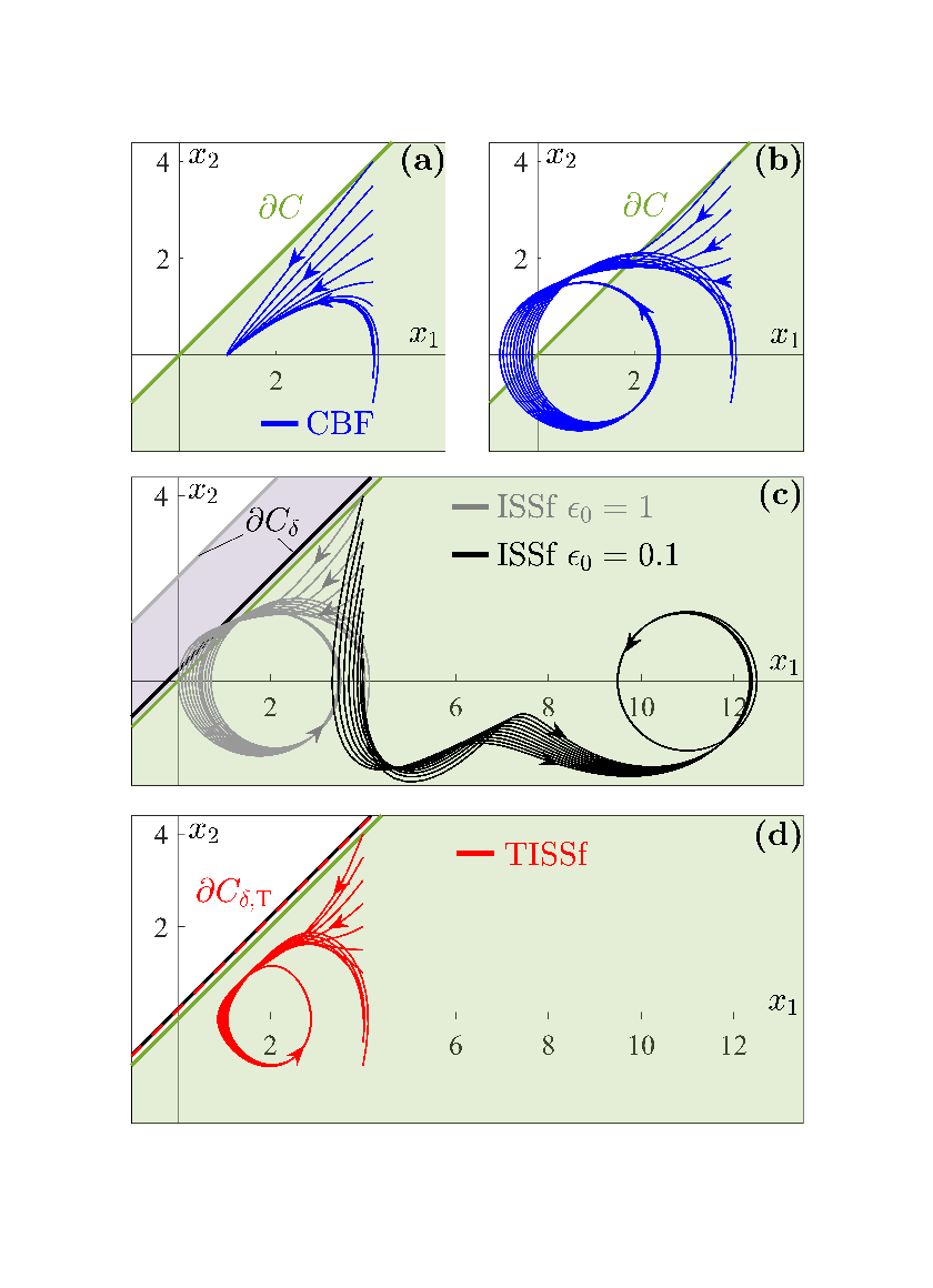
that is, choosing the extended class 𝒦∞\mathcal{K}_{\infty} function α⁡(r)=r{\alpha(r)=r} yields that k​(𝐱)∈KCBF​(𝐱){k(\mathbf{x})\in K_{\textrm{CBF}}(\mathbf{x})}. We present simulation results for the closed loop system in Fig. 1(a), where all the trajectories initiated from different initial conditions 𝐱⁡(0)∈𝒞{\mathbf{x}(0)\in\mathcal{C}} safely approach the stable equilibrium point (1,0)(1,0).

II-B Input-to-State Safety

Unmodeled effects and disturbances may make it infeasible for a state feedback controller 𝐤⁡(𝐱){\mathbf{k}(\mathbf{x})} to be implemented exactly. Instead, a potentially time-varying disturbance 𝐝:ℝ≥0→ℝm{\mathbf{d}:\mathbb{R}_{\geq 0}\to\mathbb{R}^{m}} is added to the controller, such that 𝐮=𝐤⁡(𝐱)+𝐝⁡(t){\mathbf{u}=\mathbf{k}(\mathbf{x})+\mathbf{d}(t)}, resulting in the closed loop system:

𝐱˙=𝐟⁡(𝐱)+𝐠⁡(𝐱)​𝐤​(𝐱)+𝐠⁡(𝐱)​𝐝​(t).\dot{\mathbf{x}}=\mathbf{f}(\mathbf{x})+\mathbf{g}(\mathbf{x})\mathbf{k}(\mathbf{x})+\mathbf{g}(\mathbf{x})\mathbf{d}(t). (12)

The safety guarantees endowed by controllers satisfying 𝐤​(𝐱)∈KCBF​(𝐱){\mathbf{k}(\mathbf{x})\in K_{\textrm{CBF}}(\mathbf{x})} may no longer be valid for the disturbed closed loop system. Thus, we wish to design a safety-critical controller that ensures safety in the presence of disturbances. We consider the disturbed control system:

𝐱˙=𝐟⁡(𝐱)+𝐠⁡(𝐱)​𝐮+𝐠⁡(𝐱)​𝐝​(t),\dot{\mathbf{x}}=\mathbf{f}(\mathbf{x})+\mathbf{g}(\mathbf{x})\mathbf{u}+\mathbf{g}(\mathbf{x})\mathbf{d}(t), (13)

where the disturbance 𝐝\mathbf{d} is assumed to be bounded, that is, ‖𝐝‖∞=supt≥0‖𝐝⁡(t)‖<∞{\|\mathbf{d}\|_{\infty}=\sup_{t\geq 0}\|\mathbf{d}(t)\|<\infty}. With disturbances, we look for a larger set 𝒞δ⊂ℝn{\mathcal{C}_{{\delta}}\subset\mathbb{R}^{n}} parameterized by δ≥0\delta\geq 0, i.e., 𝒞⊆𝒞δ{\mathcal{C}\subseteq\mathcal{C}_{{\delta}}}, that is forward invariant for all 𝐝\mathbf{d} satisfying ‖𝐝‖∞≤δ{\|\mathbf{d}\|_{\infty}\leq\delta}. We require 𝒞δ\mathcal{C}_{{\delta}} to grow monotonically with δ{\delta}, and recover the original safe set in the absence of the disturbance, i.e., 𝒞δ≡𝒞{\mathcal{C}_{{\delta}}\equiv\mathcal{C}} when δ=0{{\delta=0}}. Thus, define a function hδ:ℝn×ℝ≥0→ℝ{h_{{\delta}}:\mathbb{R}^{n}\times\mathbb{R}_{\geq 0}\to\mathbb{R}} as:

hδ​(𝐱,δ)≜h⁡(𝐱)+γ⁡(δ),h_{{\delta}}(\mathbf{x},{\delta})\triangleq h(\mathbf{x})+\gamma({\delta}), (14)

with γ∈𝒦∞{\gamma\in\mathcal{K}_{\infty}} and define 𝒞δ\mathcal{C}_{{\delta}} as its 0-superlevel set:

𝒞δ\displaystyle\mathcal{C}_{{\delta}} ≜{𝐱∈ℝn:hδ​(𝐱,δ)≥0},\displaystyle\triangleq\left\{\mathbf{x}\in\mathbb{R}^{n}:h_{{\delta}}(\mathbf{x},{\delta})\geq 0\right\}, (15)
∂𝒞δ\displaystyle\partial\mathcal{C}_{{\delta}} ≜{𝐱∈ℝn:hδ​(𝐱,δ)=0},\displaystyle\triangleq\{\mathbf{x}\in\mathbb{R}^{n}:h_{{\delta}}(\mathbf{x},{\delta})=0\}, (16)
Int​(𝒞δ)\displaystyle\textrm{Int}(\mathcal{C}_{{\delta}}) ≜{𝐱∈ℝn:hδ​(𝐱,δ)>0}.\displaystyle\triangleq\{\mathbf{x}\in\mathbb{R}^{n}:h_{{\delta}}(\mathbf{x},{\delta})>0\}. (17)
Definition 2 (Input-to-State Safety).

Let 𝒞⊂ℝn{\mathcal{C}\subset\mathbb{R}^{n}} be the 0-superlevel set of a continuously differentiable function h:ℝn→ℝ{h:\mathbb{R}^{n}\to\mathbb{R}}. The system (12) is input-to-state safe (ISSf) if there exists γ∈𝒦∞{\gamma\in\mathcal{K}_{\infty}} and δ≥0\delta\geq 0 such that for all 𝐝\mathbf{d} satisfying ‖𝐝‖∞≤δ{\|\mathbf{d}\|_{\infty}\leq\delta}, the set 𝒞δ\mathcal{C}_{{\delta}} defined by (15) is forward invariant. In this case, we refer to the original set 𝒞\mathcal{C} as an input-to-state safe set (ISSf set).

Given a controller 𝐤⁡(𝐱){\mathbf{k}(\mathbf{x})} that makes the undisturbed system (2) safe with respect to the set 𝒞\mathcal{C} for a given CBF hh, i.e., 𝐤​(𝐱)∈KCBF​(𝐱){{\mathbf{k}(\mathbf{x})\in K_{\textrm{CBF}}(\mathbf{x})}}, we consider the following modification:

𝐮=𝐤⁡(𝐱)+1ϵ0​L𝐠​h​(𝐱)⊤,\mathbf{u}=\mathbf{k}(\mathbf{x})+\frac{1}{\epsilon_{0}}L_{\mathbf{g}}h(\mathbf{x})^{\top}, (18)

where ϵ0∈ℝ>0{\epsilon_{0}\in\mathbb{R}_{>0}} is a positive constant. Motivated by this controller, we give the definition of the input-to-state safe control barrier function:

Definition 3 (Input-to-State Safe Control Barrier Function (ISSf-CBF)).

Let 𝒞⊂ℝn{\mathcal{C}\subset\mathbb{R}^{n}} be the 0-superlevel set of a continuously differentiable function h:ℝn→ℝ{h:\mathbb{R}^{n}\to\mathbb{R}} with ∂h∂𝐱​(𝐱)≠𝟎{\frac{\partial h}{\partial\mathbf{x}}(\mathbf{x})\neq\mathbf{0}} when h⁡(𝐱)=0{h(\mathbf{x})=0}. Then hh is an input-to-state safe control barrier function (ISSf-CBF) for (13) on 𝒞\mathcal{C} if there exists α∈𝒦∞,e{\alpha\in\mathcal{K}_{\infty,\rm e}} and ϵ0>0{\epsilon_{0}>0} such that for all 𝐱∈ℝn{\mathbf{x}\in\mathbb{R}^{n}}:

sup𝐮∈ℝm[L𝐟​h​(𝐱)+L𝐠​h​(𝐱)​𝐮]>−α⁡(h⁡(𝐱))+‖L𝐠​h​(𝐱)‖2ϵ0.\sup_{\mathbf{u}\in\mathbb{R}^{m}}\left[L_{\mathbf{f}}h(\mathbf{x})+L_{\mathbf{g}}h(\mathbf{x})\mathbf{u}\right]>-\alpha(h(\mathbf{x}))+\frac{\|L_{\mathbf{g}}h(\mathbf{x})\|^{2}}{\epsilon_{0}}. (19)

As with CBFs, we may define the point-wise set of control values satisfying (19):

KISSf(𝐱)≜{𝐮∈ℝm|h˙(𝐱,𝐮)≥−α(h(𝐱))+‖L𝐠​h​(𝐱)‖2ϵ0}.{K_{\textrm{ISSf}}(\mathbf{x})\triangleq\left\{\mathbf{u}\in\mathbb{R}^{m}~\left|~\dot{h}(\mathbf{x},\mathbf{u})\geq-\alpha(h(\mathbf{x}))+\frac{\|L_{\mathbf{g}}h(\mathbf{x})\|^{2}}{\epsilon_{0}}\right.\right\}.}

(20)
Theorem 2 ([15]).

Let 𝒞⊂ℝn{\mathcal{C}\subset\mathbb{R}^{n}} be the 0-superlevel set of a continuously differentiable function h:ℝn→ℝ{h:\mathbb{R}^{n}\to\mathbb{R}} with ∂h∂𝐱​(𝐱)≠𝟎{\frac{\partial h}{\partial\mathbf{x}}(\mathbf{x})\neq\mathbf{0}} when h⁡(𝐱)=0{h(\mathbf{x})=0} and δ≥0\delta\geq 0. If hh is an ISSf-CBF for (13) on 𝒞\mathcal{C}, then for any Lipschitz continuous controller with 𝐤⁡(𝐱)∈KISSf{\mathbf{k}(\mathbf{x})\in K_{\rm ISSf}} for all 𝐱∈ℝn{\mathbf{x}\in\mathbb{R}^{n}} and for all 𝐝\mathbf{d} satisfying ‖𝐝‖∞≤δ{\|\mathbf{d}\|_{\infty}\leq\delta}, the system (12) is safe with respect to 𝒞δ\mathcal{C}_{{\delta}} defined as in (15) with γ∈𝒦∞{\gamma\in\mathcal{K}_{\infty}} defined as:

γ⁡(δ)≜−α−1​(−ϵ0​δ24),\gamma({\delta})\triangleq-\alpha^{-1}\left(-\frac{\epsilon_{0}{\delta}^{2}}{4}\right), (21)

where α−1∈𝒦∞,e{\alpha^{-1}\in\mathcal{K}_{\infty,{\rm e}}}. This implies 𝒞\mathcal{C} is an ISSf set.

Remark 1.

The original ISSf-CBF definition proposed in [15] requires the condition:

sup𝐮∈ℝm[L𝐟​h​(𝐱)+L𝐠​h​(𝐱)​(𝐮+𝐝)]>−α⁡(h⁡(𝐱))−ι⁡(‖𝐝‖∞),\sup_{\mathbf{u}\in\mathbb{R}^{m}}\left[L_{\mathbf{f}}h(\mathbf{x})+L_{\mathbf{g}}h(\mathbf{x})(\mathbf{u+d})\right]>-\alpha(h(\mathbf{x}))-\iota(\|\mathbf{d}\|_{\infty}), (22)

for some ι∈𝒦∞{\iota\in\mathcal{K}_{\infty}}. It also proves that a function satisfying (19) meets the condition in (22) for ι\iota defined as:

ι⁡(‖𝐝‖∞)≜ϵ0​‖𝐝‖∞24.\iota(\|\mathbf{d}\|_{\infty})\triangleq\frac{\epsilon_{0}\|\mathbf{d}\|_{\infty}^{2}}{4}. (23)

We use the more specific definition in (19) as it is better suited for the controller design presented in this letter.

As α−1∈𝒦∞,e{\alpha^{-1}\in\mathcal{K}_{\infty,{\rm e}}}, a smaller ϵ0\epsilon_{0} implies a smaller value of γ⁡(δ){\gamma({\delta})} for a given δ≥0{\delta\geq 0}, which reduces the difference between the sets 𝒞\mathcal{C} and 𝒞δ\mathcal{C}_{{\delta}}. However, taking ϵ0\epsilon_{0} to be small increases the right hand side of (19), and forces a more restrictive safety condition to be met by 𝐤\mathbf{k}. Controllers satisfying this more restrictive condition may lead to undesirable performance as illustrated by the example below.
Refer to caption
Fig. 1: The sets 𝒞\mathcal{C}, 𝒞δ\mathcal{C}_{{\delta}} and 𝒞δ,T\mathcal{C}_{{\delta},\rm T} (shaded) and simulation results for Examples 1-3. (a) The boundary ∂𝒞\partial\mathcal{C} (green) and simulated trajectories with controller (9) without disturbance. (b) Trajectories with disturbance. (c) The boundary ∂𝒞δ\partial\mathcal{C}_{{\delta}} for ϵ0=0.1{\epsilon_{0}=0.1} (gray) and ϵ0=1{\epsilon_{0}=1} (black) and simulation results for controller (25). (d) The boundary ∂𝒞δ,T\partial\mathcal{C}_{{\delta},\rm T} (red) and simulation results for controller (45).
Example 2.

We now introduce a disturbance to the example:

x˙1=−x2,x˙2=u+d⁡(t),\dot{x}_{1}=-x_{2},\quad\dot{x}_{2}=u+d(t), (24)

where d:ℝ≥0→ℝ{d:\mathbb{R}_{\geq 0}\to\mathbb{R}}. Fig. 1(b) depicts the simulation results with the controller k⁡(𝐱)k(\mathbf{x}) defined in (9) for the harmonic disturbance d⁡(t)=δ​sin⁡t{d(t)={\delta}\sin{t}} with δ=3{{\delta}=3}. We see that the disturbance makes the state trajectories leave 𝒞\mathcal{C} periodically. According to (18), we consider the modified controller:

u=k⁡(𝐱)+L𝐠​h​(𝐱)ϵ0=x1−2​x2−1−1ϵ0,u=k(\mathbf{x})+\frac{L_{\mathbf{g}}h(\mathbf{x})}{\epsilon_{0}}=x_{1}-2x_{2}-1-\frac{1}{\epsilon_{0}}, (25)

cf. (9). The evolution of hh under (12) is given by:

L𝐟​h​(𝐱)+L𝐠​h​(𝐱)​k​(𝐱)=−x1+x2⏟−h⁡(𝐱)+1+1ϵ0>−h⁡(𝐱)+1ϵ0,L_{\mathbf{f}}h(\mathbf{x})+L_{\mathbf{g}}h(\mathbf{x})k(\mathbf{x})=\underbrace{-x_{1}+x_{2}}_{-h(\mathbf{x})}+1+\frac{1}{\epsilon_{0}}>-h(\mathbf{x})+\frac{1}{\epsilon_{0}},

such that with α⁡(r)=r{\alpha(r)=r}, hh is an ISSf-CBF for (24) on the set 𝒞\mathcal{C} defined in (11). Furthermore, with −α−1​(−r)=r{-\alpha^{-1}(-r)=r}, we have γ⁡(δ)=ϵ0​δ24{\gamma({\delta})=\frac{\epsilon_{0}{\delta}^{2}}{4}}, yielding:

𝒞δ={𝐱∈ℝ2|x1−x2+ϵ0​δ24≥0}.\mathcal{C}_{{\delta}}=\left\{\mathbf{x}\in\mathbb{R}^{2}~\left|~x_{1}-x_{2}+\frac{\epsilon_{0}{\delta}^{2}}{4}\geq 0\right.\right\}. (26)

Figure 1(c) portrays the boundary ∂𝒞δ\partial\mathcal{C}_{{\delta}} for ϵ0=1{\epsilon_{0}=1} (gray) and ϵ0=0.1{\epsilon_{0}=0.1} (black). A larger ϵ0\epsilon_{0} implies a larger gap between the original set 𝒞\mathcal{C} and the forward invariant set 𝒞δ\mathcal{C}_{{\delta}}, and as a result, gives way to the trajectories leaving 𝒞\mathcal{C}. In contrast, a smaller ϵ0\epsilon_{0} shifts 𝒞δ\mathcal{C}_{{\delta}} closer to 𝒞\mathcal{C}, yielding trajectories that stay in 𝒞\mathcal{C}. This, however, comes with an expense of substantially effecting the performance as the trajectories are pushed further inside 𝒞\mathcal{C}.

III Main Result

In this section, we present the main result of the paper by introducing a new method for characterizing safety in the presence of disturbances. It uses a more general definition of the set 𝒞δ\mathcal{C}_{{\delta}} to enable synthesis of controllers that can ensure safety without compromising performance.

The previous specification of hδh_{{\delta}} and γ\gamma as in (14) and (21), respectively, implies that the difference hδ​(𝐱)−h​(𝐱){h_{{\delta}}(\mathbf{x})-h(\mathbf{x})} is constant for all 𝐱∈𝒞δ\mathbf{x}\in\mathcal{C}_{{\delta}} for a given δ{\delta}. In other words, requiring a constant ϵ0\epsilon_{0} imposes strong restrictions on the structure of hδ​(𝐱)h_{{\delta}}(\mathbf{x}) and 𝒞δ\mathcal{C}_{{\delta}}. As a result, prioritizing safety with a smaller ϵ0\epsilon_{0} may lead to overcompensation and may affect the performance in an undesirable fashion. We wish to find a new set that is still forward invariant, but allows more flexibility in designing controllers. To this end, define the function hδ,T:ℝn×ℝ≥0→ℝh_{{\delta},T}:\mathbb{R}^{n}\times\mathbb{R}_{\geq 0}\to\mathbb{R} as:

hδ,T​(𝐱,δ)=h⁡(𝐱)+γT​(h⁡(𝐱),δ),h_{{\delta},\rm T}(\mathbf{x},{\delta})=h(\mathbf{x})+\gamma_{\rm T}(h(\mathbf{x}),{\delta}), (27)

with γT:ℝ×ℝ≥0→ℝ≥0{\gamma_{\rm T}:\mathbb{R}\times\mathbb{R}_{\geq 0}\to\mathbb{R}_{\geq 0}} continuously differentiable in its first argument and γT​(a,⋅)∈𝒦∞{\gamma_{\rm T}(a,\cdot)\in\mathcal{K}_{\infty}} for all a∈ℝ{a\in\mathbb{R}}. Indeed, hδh_{{\delta}} defined by (14) is a special case of hδ,Th_{{\delta},\rm T} defined by (27). We define 𝒞δ,T\mathcal{C}_{{\delta},\rm T} as the 0-superlevel set of the function hδ,Th_{{\delta},\rm T}:

𝒞δ,T\displaystyle\mathcal{C}_{{\delta},\rm T} ≜{𝐱∈ℝn:hδ,T​(𝐱,δ)≥0},\displaystyle\triangleq\left\{\mathbf{x}\in\mathbb{R}^{n}:h_{{\delta},\rm T}(\mathbf{x},{\delta})\geq 0\right\}, (28)
∂𝒞δ,T\displaystyle\partial\mathcal{C}_{{\delta},\rm T} ≜{𝐱∈ℝn:hδ,T​(𝐱,δ)=0},\displaystyle\triangleq\{\mathbf{x}\in\mathbb{R}^{n}:h_{{\delta},\rm T}(\mathbf{x},{\delta})=0\}, (29)
Int​(𝒞δ,T)\displaystyle\textrm{Int}(\mathcal{C}_{{\delta},\rm T}) ≜{𝐱∈ℝn:hδ,T​(𝐱,δ)>0}.\displaystyle\triangleq\{\mathbf{x}\in\mathbb{R}^{n}:h_{{\delta},\rm T}(\mathbf{x},{\delta})>0\}. (30)

Note that 𝒞⊂𝒞δ,T{\mathcal{C}\subset\mathcal{C}_{{\delta},\rm T}} for δ>0{\delta}>0. In the absence of disturbances (δ=0{{\delta}=0}) we recover the original set (𝒞δ,T≡𝒞){(\mathcal{C}_{{\delta},\rm T}\equiv\mathcal{C})} as hδ,T​(𝐱,0)=h⁡(𝐱){h_{{\delta},\rm T}(\mathbf{x},0)=h(\mathbf{x})}. Also, 𝒞δ,T\mathcal{C}_{{\delta},\rm T} grows monotonically with δ{\delta}. Analogous to (18), we propose the controller:

𝐮=𝐤⁡(𝐱)+1ϵ⁡(h⁡(𝐱))​L𝐠​h​(𝐱)⊤,\mathbf{u}=\mathbf{k}(\mathbf{x})+\frac{1}{\epsilon(h(\mathbf{x}))}L_{\mathbf{g}}h(\mathbf{x})^{\top}, (31)

where ϵ:ℝ→ℝ>0{\epsilon:\mathbb{R}\to\mathbb{R}_{>0}} is a continuously differentiable function and 𝐤​(𝐱)∈KCBF​(𝐱){\mathbf{k}(\mathbf{x})\in K_{\textrm{CBF}}(\mathbf{x})}. This controller motivates a generalization of Definition 3, and a corresponding safety result.

Definition 4 (Tunable Input-to-State Safe Control Barrier Function (TISSf-CBF)).

Let 𝒞⊂ℝn{\mathcal{C}\subset\mathbb{R}^{n}} be the 0-superlevel set of a continuously differentiable function h:ℝn→ℝ{h:\mathbb{R}^{n}\to\mathbb{R}} with ∂h∂𝐱​(𝐱)≠𝟎{\frac{\partial h}{\partial\mathbf{x}}(\mathbf{x})\neq\mathbf{0}} when h⁡(𝐱)=0{h(\mathbf{x})=0}. Then hh is a tunable input-to-state safe control barrier function (TISSf-CBF) for (13) on 𝒞\mathcal{C} with continuously differentiable function ϵ:ℝ→ℝ>0{\epsilon:\mathbb{R}\to\mathbb{R}_{>0}} if there exists α∈𝒦∞,e{\alpha\in\mathcal{K}_{\infty,\rm e}} such that for all 𝐱∈ℝn{\mathbf{x}\in\mathbb{R}^{n}}:

sup𝐮∈ℝm[L𝐟​h​(𝐱)+L𝐠​h​(𝐱)​𝐮]>−α⁡(h⁡(𝐱))+‖L𝐠​h​(𝐱)‖2ϵ⁡(h⁡(𝐱)).\sup_{\mathbf{u}\in\mathbb{R}^{m}}\left[L_{\mathbf{f}}h(\mathbf{x})+L_{\mathbf{g}}h(\mathbf{x})\mathbf{u}\right]>-\alpha(h(\mathbf{x}))+\frac{\|L_{\mathbf{g}}h(\mathbf{x})\|^{2}}{\epsilon(h(\mathbf{x}))}. (32)

As with ISSf-CBFs, we may define the point-wise set of control values satisfying (32):

KTISSf(𝐱)≜{𝐮∈ℝm|h˙(𝐱,𝐮)≥−α(h(𝐱))+‖L𝐠​h​(𝐱)‖2ϵ⁡(h⁡(𝐱))}.{K_{\textrm{TISSf}}(\mathbf{x})\triangleq\left\{\mathbf{u}\in\mathbb{R}^{m}~\left|~\dot{h}(\mathbf{x},\mathbf{u})\geq-\alpha(h(\mathbf{x}))+\frac{\|L_{\mathbf{g}}h(\mathbf{x})\|^{2}}{\epsilon(h(\mathbf{x}))}\right.\right\}.}

(33)
Theorem 3.

Let 𝒞⊂ℝn{\mathcal{C}\subset\mathbb{R}^{n}} be the 0-superlevel set of a continuously differentiable function h:ℝn→ℝ{h:\mathbb{R}^{n}\to\mathbb{R}} and δ≥0\delta\geq 0. If hh is a TISSf-CBF for (13) on 𝒞\mathcal{C} with continuously differentiable function ϵ:ℝ→ℝ>0{\epsilon:\mathbb{R}\to\mathbb{R}_{>0}} such that α−1∈𝒦∞,e{\alpha^{-1}\in\mathcal{K}_{\infty,\rm e}} is continuously differentiable and ϵ\epsilon satisfies:

d​ϵd​r​(h​(𝐱))≥0,\frac{\mathrm{d}\epsilon}{\mathrm{d}r}(h(\mathbf{x}))\geq 0, (34)

then for any Lipschitz continuous controller with 𝐤​(𝐱)∈KTISSf​(𝐱){\mathbf{k}(\mathbf{x})\in K_{\rm TISSf}(\mathbf{x})} for all 𝐱∈ℝn{\mathbf{x}\in\mathbb{R}^{n}} and for all 𝐝\mathbf{d} satisfying ‖𝐝‖∞≤δ{\|\mathbf{d}\|_{\infty}\leq\delta}, the system (12) is safe with respect to 𝒞δ,T\mathcal{C}_{{\delta},T} defined as in (28)-(30) with γT:ℝ×ℝ≥0{\gamma_{\rm T}:\mathbb{R}\times\mathbb{R}_{\geq 0}} defined as:

γT​(h⁡(𝐱),δ)≜−α−1​(−ϵ⁡(h⁡(𝐱))​δ24).\gamma_{\rm T}(h(\mathbf{x}),{\delta})\triangleq-\alpha^{-1}\left(-\frac{\epsilon(h(\mathbf{x})){\delta}^{2}}{4}\right). (35)
Proof.

Our goal is to show that the set 𝒞δ,T\mathcal{C}_{{\delta},\rm T} defined by (28)-(30) is forward invariant. For a controller satisfying 𝐤​(𝐱)∈KTISSf​(𝐱){\mathbf{k}(\mathbf{x})\in K_{\textrm{TISSf}}(\mathbf{x})} for all 𝐱∈ℝn{\mathbf{x}\in\mathbb{R}^{n}}, we have:

h˙​(𝐱,t)=L𝐟​h​(𝐱)+L𝐠​h​(𝐱)​(𝐤⁡(𝐱)+𝐝⁡(t))≥−α⁡(h⁡(𝐱))+‖L𝐠​h​(𝐱)‖2ϵ⁡(h⁡(𝐱))+L𝐠​h​(𝐱)​𝐝​(t).\begin{split}\dot{h}(\mathbf{x},t)=&L_{\mathbf{f}}h(\mathbf{x})+L_{\mathbf{g}}h(\mathbf{x})(\mathbf{k}(\mathbf{x})+\mathbf{d}(t))\\ \geq&-\alpha(h(\mathbf{x}))+\frac{\|L_{\mathbf{g}}h(\mathbf{x})\|^{2}}{\epsilon(h(\mathbf{x}))}+L_{\mathbf{g}}h(\mathbf{x})\mathbf{d}(t).\end{split} (36)

Noting that:

L𝐠​h​(𝐱)​𝐝​(t)≥−‖L𝐠​h​(𝐱)‖​‖𝐝‖∞≥−‖L𝐠​h​(𝐱)‖​δL_{\mathbf{g}}h(\mathbf{x})\mathbf{d}(t)\geq-\|L_{\mathbf{g}}h(\mathbf{x})\|\|\mathbf{d}\|_{\infty}{\geq-\|L_{\mathbf{g}}h(\mathbf{x})\|\delta}

and ϵ⁡(h⁡(𝐱))>0{\epsilon(h(\mathbf{x}))>0} for all 𝐱∈ℝn{\mathbf{x}\in\mathbb{R}^{n}} and t≥0{t\geq 0}, adding and subtracting ϵ⁡(h⁡(𝐱))​δ24{\frac{\epsilon(h(\mathbf{x})){\delta}^{2}}{4}}, and completing the squares yields:

h˙​(𝐱,t)≥−α⁡(h⁡(𝐱))−ϵ⁡(h⁡(𝐱))​δ24.\dot{h}(\mathbf{x},t)\geq-\alpha(h(\mathbf{x}))-\frac{\epsilon(h(\mathbf{x})){\delta}^{2}}{4}. (37)

Next, taking the time derivative of the function hδ,T{h_{{\delta},\rm T}} defined by (27) yields:

h˙δ,T​(𝐱,δ,t)=(1+∂γT∂h​(h⁡(𝐱),δ))​h˙​(𝐱,t).\displaystyle\dot{h}_{{\delta},\rm T}(\mathbf{x},{\delta},t)=\left(1+\frac{\partial\gamma_{\rm T}}{\partial h}(h(\mathbf{x}),{\delta})\right)\dot{h}(\mathbf{x},t). (38)

As ϵ\epsilon satisfies (34) and γT\gamma_{\rm T} is defined as in (35), we have:

1+∂γT∂h​(h⁡(𝐱),δ)>0.1+\frac{\partial\gamma_{\rm T}}{\partial h}(h(\mathbf{x}),{\delta})>0. (39)

Substituting (37) into (38), we obtain:

h˙δ,T​(𝐱,δ,t)≥(1+∂γT∂h​(h⁡(𝐱),δ))​(−α⁡(h⁡(𝐱))−ϵ⁡(h⁡(𝐱))​δ24).\begin{split}&\dot{h}_{{\delta},\rm T}(\mathbf{x},{\delta},t)\geq\\ &\left(1+\frac{\partial\gamma_{\rm T}}{\partial h}(h(\mathbf{x}),{\delta})\right)\left(-\alpha(h(\mathbf{x}))-\frac{\epsilon(h(\mathbf{x})){\delta}^{2}}{4}\right).\end{split}

Next, we consider a state 𝐱∈∂𝒞δ,T{\mathbf{x}\in\partial\mathcal{C}_{{\delta},\rm T}}, such that hδ,T​(𝐱)=0{h_{{\delta},\rm T}(\mathbf{x})=0}, for which (27) and (35) imply:

−α⁡(h⁡(𝐱))−ϵ⁡(h⁡(𝐱))​δ24=0,-\alpha(h(\mathbf{x}))-\frac{\epsilon(h(\mathbf{x})){\delta}^{2}}{4}=0, (40)

yielding:

h˙δ,T​(𝐱,δ,t)≥0.\dot{h}_{{\delta},\rm T}(\mathbf{x},{\delta},t)\geq 0. (41)

Additionally, we have −α⁡(h⁡(𝐱))≥0{-\alpha(h(\mathbf{x}))\geq 0} when hδ,T​(𝐱)=0{h_{{\delta},\rm T}(\mathbf{x})=0} by construction. Thus, the strict inequality in (32) requires that ∂h∂𝐱​(𝐱)≠𝟎{\frac{\partial h}{\partial\mathbf{x}}(\mathbf{x})\neq\mathbf{0}} for 𝐱∈∂𝒞δ,T{\mathbf{x}\in\partial\mathcal{C}_{\delta,T}}. Finally, we have:

∂hδ,T∂𝐱​(𝐱,δ)=(1+∂γT∂h​(h​(𝐱),δ))⏟>0​∂h∂𝐱​(𝐱)≠0,\frac{\partial h_{{\delta},\rm T}}{\partial\mathbf{x}}(\mathbf{x},{\delta})=\underbrace{\left(1+\frac{\partial\gamma_{\rm T}}{\partial h}(h(\mathbf{x}),{\delta})\right)}_{>0}\frac{\partial h}{\partial\mathbf{x}}(\mathbf{x})\neq 0, (42)

using (39). Therefore, Nagumo’s theorem [18] implies the set 𝒞δ,T\mathcal{C}_{{\delta},\rm T} is forward invariant as hδ,T​(𝐱,δ)=0{h_{{\delta},\rm T}(\mathbf{x},{\delta})=0} implies h˙δ,T​(𝐱,δ,t)≥0{\dot{h}_{{\delta},\rm T}(\mathbf{x},{\delta},t)\geq 0}, and ∂hδ,T∂𝐱​(𝐱,δ)≠0{\frac{\partial h_{{\delta},\rm T}}{\partial\mathbf{x}}(\mathbf{x},{\delta})\neq 0}. ∎

Remark 2.

We note that the condition on ϵ\epsilon in (34) is stronger than necessary, but is an easily verifiable design condition. In particular, ϵ\epsilon only needs to satisfy that for δ>0\delta>0 and 𝐱∈ℝn{\mathbf{x}\in\mathbb{R}^{n}}:

d​ϵd​r​(h⁡(𝐱))>−4δ2​1Dα−1(−ϵ(h(𝐱))δ2/4).\frac{\mathrm{d}\epsilon}{\mathrm{d}r}(h(\mathbf{x}))>-\frac{4}{{\delta}^{2}}\dfrac{1}{D\alpha^{-1}(-\epsilon(h(\mathbf{x}))\delta^{2}/4)}. (43)

Noting that α−1∈𝒦∞,e{\alpha^{-1}\in\mathcal{K}_{\infty,{\rm e}}} and is continuously differentiable implies 0≤Dα−1(−ϵ(h(𝐱))δ2/4)<∞{0\leq D\alpha^{-1}(-\epsilon(h(\mathbf{x}))\delta^{2}/4)<\infty} for all 𝐱∈ℝn{\mathbf{x}\in\mathbb{R}^{n}}. The right-hand side of (43) approaches −∞-\infty as δ→0{\delta\to 0} or Dα−1(−ϵ(h(𝐱))δ2/4)→0{D\alpha^{-1}(-\epsilon(h(\mathbf{x}))\delta^{2}/4)\to 0}, making ϵ\epsilon unconstrained.

Example 3.

For the disturbed system in Example 2 with δ=3{\delta=3}, we pick the following differentiable function:

ϵ⁡(h⁡(𝐱))≜ϵ0​eλ​h​(𝐱),\epsilon(h(\mathbf{x}))\triangleq\epsilon_{0}{\rm e}^{{\lambda}h(\mathbf{x})}, (44)

with constants ϵ0,λ∈ℝ>0{\epsilon_{0},{\lambda}\in\mathbb{R}_{>0}}. Considering the controller:

u=k⁡(𝐱)+L𝐠​h​(𝐱)ϵ⁡(h⁡(𝐱))=x1−2​x2−1−1ϵ0​eλ⁡(x1−x2),u=k(\mathbf{x})+\frac{L_{\mathbf{g}}h(\mathbf{x})}{\epsilon(h(\mathbf{x}))}=x_{1}-2x_{2}-1-\frac{1}{\epsilon_{0}{\rm e}^{{\lambda}(x_{1}-x_{2})}}, (45)

it can be shown that hh as defined in (10) is a TISSf-CBF for α⁡(r)=r{\alpha(r)=r}. Furthermore, the choice of the function ϵ\epsilon with ϵ0,λ>0{\epsilon_{0},\lambda>0} in (44) satisfies the condition (34). Thus, the set:

𝒞δ,T={𝐱∈ℝ2|x1−x2+ϵ0​eλ⁡(x1−x2)​δ24≥0},\mathcal{C}_{{\delta},\rm T}=\left\{\mathbf{x}\in\mathbb{R}^{2}~\left|~x_{1}-x_{2}+\frac{\epsilon_{0}{\rm e}^{\lambda(x_{1}-x_{2})}{\delta}^{2}}{4}\geq 0\right.\right\},

(46)

is forward invariant. It is noted that λ=0{\lambda=0} recovers ISSf setup with ϵ⁡(h⁡(𝐱))≡ϵ0{\epsilon(h(\mathbf{x}))\equiv\epsilon_{0}}, whereas a larger λ\lambda pulls 𝒞δ,T\mathcal{C}_{{\delta},\rm T} closer to the safe set 𝒞\mathcal{C}, and decreases the effect of the corresponding term in the controller (45) for h⁡(𝐱)>0{h(\mathbf{x})>0}. We depict the set 𝒞δ,T\mathcal{C}_{{\delta},\rm T} in Fig. 1(d) considering ϵ0=e−2{\epsilon_{0}=\rm{e}^{-2}}, λ=2{\lambda=2} and along with simulation results. All solution trajectories stay within the set 𝒞δ,T\mathcal{C}_{{\delta},\rm T} that is close to 𝒞\mathcal{C}, and the overcompensation inside the set 𝒞\mathcal{C} is prevented as ϵ⁡(h⁡(𝐱))\epsilon(h(\mathbf{x})) takes larger values when h⁡(𝐱)≫0{h(\mathbf{x})\gg 0}.

Remark 3.

Ensuring the forward invariance of a slightly larger set suggests modifying the set 𝒞\mathcal{C} in the presence of a disturbance. Specifically, considering a set 𝒞¯⊆𝒞\overline{\mathcal{C}}\subseteq\mathcal{C} such that 𝒞¯δ,T⊆𝒞\overline{\mathcal{C}}_{\delta,\rm T}\subseteq\mathcal{C} implies the safety of the original set 𝒞\mathcal{C}.

Remark 4.

Rather than utilizing (31) by modifying an existing safe controller 𝐤​(𝐱)∈KCBF​(𝐱){\mathbf{k}(\mathbf{x})\in K_{\textrm{CBF}}(\mathbf{x})}, the condition (32) can be utilized to synthesize an optimization-based controller via the following quadratic program:

𝐤QP​(𝐱)=\displaystyle\mathbf{k}_{\rm QP}(\mathbf{x})= argmin𝐮∈ℝm12​‖𝐮−𝐤⁡(𝐱)‖2\displaystyle\,\,\underset{\mathbf{u}\in\mathbb{R}^{m}}{\argmin}\quad\frac{1}{2}\|\mathbf{u}-\mathbf{k}(\mathbf{x})\|^{2} (TISSf-QP)
s.t.\displaystyle\mathrm{s.t.}\quad L𝐟​h​(𝐱)+L𝐠​h​(𝐱)​𝐮>−α⁡(h⁡(𝐱))+‖L𝐠​h​(𝐱)‖2ϵ⁡(h⁡(𝐱)),\displaystyle L_{\mathbf{f}}h(\mathbf{x})+L_{\mathbf{g}}h(\mathbf{x})\mathbf{u}>-\alpha(h(\mathbf{x}))+\frac{\|L_{\mathbf{g}}h(\mathbf{x})\|^{2}}{\epsilon(h(\mathbf{x}))},

that may intervene less compared to (31).

IV Input-to-state Safety for Automated Trucks

Here we implement previously introduced tunable input-to-state safe control barrier functions (TISSf-CBF) to design the longitudinal controller of a connected automated truck while responding to the motion of a connected vehicle ahead. We use a simplified model to design the controller and we demonstrate that it can maintain safety in real-world safety-critical scenario by simulating a high-fidelity vehicle model.

Consider the simplified model for the system:

D˙=vL−v,v˙=u+d⁡(t),v˙L=aL,\dot{D}=v_{\rm L}-v,~~~\dot{v}=u+d(t),~~~\dot{v}_{\rm L}=a_{\rm L}, (47)

where DD denotes the bumper-to-bumper headway distance between the truck and the vehicle ahead, vv is the longitudinal velocity of the truck, while vLv_{\rm L} and aLa_{\rm L} are longitudinal velocity and acceleration of the preceding vehicle. The state is defined by 𝐱=[D,v,vL]∈ℝ3{\mathbf{x}=[D,v,v_{\rm L}]\in\mathbb{R}^{3}} while uu denotes the input. The input disturbance d⁡(t)d(t) represents the unmodeled dynamics, i.e., rolling resistance, air drag, powertrain dynamics and delays related to sensing, computation and communication. We remark that while the distance DD and the velocities v,vL{v,v_{\rm L}} can be measured by sensors, to obtain the acceleration signal aLa_{\rm L} V2X communication is needed [9]. That is why we refer to the controller below as connected cruise control rather than adaptive cruise control. Finally, to incorporate physical limitations we prescribe bounds for the input and the states:

u∈[−a¯,a¯],aL∈[−a¯L,a¯L],v,vL∈[0,v¯],\displaystyle u\in[-\underline{a},\overline{a}],~~~a_{\rm L}\in[-\underline{a}_{\rm L},\overline{a}_{\rm L}],~~~v,v_{\rm L}\in[0,\overline{v}], (48)

where a¯=6​[m/s2]{\underline{a}=6~[{\rm m}/{\rm s^{2}}]}, a¯=2​[m/s2]{\overline{a}=2~[{\rm m}/{\rm s^{2}}]}, a¯L=10​[m/s2]{\underline{a}_{\rm L}=10~[{\rm m}/{\rm s^{2}}]}, a¯L=3​[m/s2]{\overline{a}_{\rm L}=3~[{\rm m}/{\rm s^{2}}]} and v¯=20​[m/s]{\overline{v}=20~[{\rm m}/{\rm s}]} are considered.

In order to ensure safety the truck needs to keep a safe distance from the preceding vehicle which may depend on the velocities. This leads to the safety function candidate:

h⁡(𝐱)=D−h^​(v,vL),h(\mathbf{x})=D-\hat{h}(v,v_{\rm L}), (49)

where we use

h^​(v,vL)=Dsf+θ​v+η​vL+ξ​v2+ζ​v​vL+ω​vL2.\hat{h}(v,v_{\rm L})=D_{\rm sf}+\theta v+\eta v_{\rm L}+\xi v^{2}+\zeta vv_{\rm L}+\omega v_{\rm L}^{2}. (50)

The parameters Dsf=2​[m]{D_{\rm sf}=2~[{\rm m}]}, θ=1.1​[s]{\theta=1.1~[{\rm s}]}, η=0.6​[s]{\eta=0.6~[{\rm s}]}, and ξ=−ζ=−ω=0.03​[s2/m]{\xi=-\zeta=-\omega=0.03~[{\rm s^{2}}/{\rm m}]} are chosen such that the truck is kept beyond a critical time headway of 1 second while considering the physical bounds (48). It can be shown that for (49)-(50) we have ∂h∂𝐱≠0{\frac{\partial h}{\partial\mathbf{x}}\neq 0} when h⁡(𝐱)=0{h(\mathbf{x})=0}.

We define the set:

𝒞={𝐱∈ℝ3|D−h^(v,vL)≥0},\mathcal{C}=\left\{\mathbf{x}\in\mathbb{R}^{3}~\left|~D-\hat{h}(v,v_{\rm L})\geq 0\right.\right\}, (51)

and to render it safe, we utilize a feedback controller

k⁡(𝐱)=k1​(V⁡(D)−v)+k2​(vL−v),k(\mathbf{x})=k_{1}(V(D)-v)+k_{2}(v_{\rm L}-v), (52)

where k1,k2∈ℝ{k_{1},k_{2}\in\mathbb{R}} are the controller parameters. The first term in (52) contains the range policy function V:ℝ→ℝ≥0{V:\mathbb{R}\to\mathbb{R}_{\geq 0}}:

V⁡(D)=max⁡{0,min⁡{κ⁡(D−Dst),v¯}},V(D)=\max\big\{0,\min\{\kappa(D-D_{\rm st}),\overline{v}\}\big\}, (53)

where DstD_{\rm st} is the desired stopping distance and 1/κ{1/\kappa} defines the desired time headway. The second term in (52) responds to the speed mismatch. Considering α⁡(r)=r{\alpha(r)=r} one may show that the parameters k1=0.7​[1/s]{k_{1}=0.7~[1/\text{s}]}, k2=0.75​[1/s]{k_{2}=0.75~[1/\text{s}]}, κ=0.7​[1/s]{\kappa=0.7~[1/\text{s}]}, Dst=7​[m]{D_{\rm st}=7~[\text{m}]} yield k⁡(𝐱)∈KCBF{k(\mathbf{x})\in K_{\rm CBF}}; see [9].

In order to incorporate real-world disturbances, numerical simulations are carried out using a high fidelity truck model built in TruckSim and Simulink. This model contains details about the engine, clutch, gearbox, tires and mechanical/hydraulic braking components which inevitably delay the realization of the longitudinal acceleration command and considered as disturbance in the simple model (47). Pre-recorded experimental data is used to represent the preceding vehicle’s speed vLv_{\rm L} and acceleration aLa_{\rm L}; see Fig. 2(b,d). In particular, the recorded data correspond to an emergency braking scenario in city traffic where the preceding vehicle decelerates from 15​[m/s]{15~{\rm[m/s]}} to a full stop with acceleration reaching −8​[m/s2]{-8~{\rm[m/s^{2}]}}. The simulation results are presented in Fig. 2 as blue curves. While the truck avoids the crash, it is unable to maintain safety (hh becomes negative in panel (c)) as the controller (52) is designed using the model (47) with no disturbance.

Refer to caption
Fig. 2: High-fidelity simulation results showing (a) distance, (b) velocities, (c) the barrier function hh defined by (49), and (d) input uu. Simulations are carried out with the CBF controller (52) (blue), the ISSf-CBF controller (54) for ϵ0=1.5{\epsilon_{0}=1.5} (black) and ϵ0=2.5{\epsilon_{0}=2.5} (gray), and the TISSf-CBF controller (56) (red).

Next we modify the controller (52) as:

kISSf​(𝐱)=k1​(V⁡(D)−v)+k2​(vL−v)−1ϵ0​∂h^∂v​(v,vL),k_{\rm ISSf}(\mathbf{x})=k_{1}(V(D)-v)+k_{2}(v_{\rm L}-v)-\frac{1}{\epsilon_{0}}\frac{\partial\hat{h}}{\partial v}(v,v_{\rm L}), (54)

(cf. (18)) where we used L𝐠​h​(𝐱)=−∂h^∂v​(v,vL){L_{\mathbf{g}}h(\mathbf{x})=-\frac{\partial\hat{h}}{\partial v}(v,v_{\rm L})}. Since hh is an ISSf-CBF for any ϵ0>0{\epsilon_{0}>0} the set:

𝒞δ={𝐱∈ℝ3|D−h^(v,vL)+ϵ0​δ24≥0},\mathcal{C}_{\delta}=\left\{\mathbf{x}\in\mathbb{R}^{3}~\left|~D-\hat{h}(v,v_{\rm L}){+\frac{\epsilon_{0}{\delta}^{2}}{4}\geq 0}\right.\right\}, (55)

is forward invariant according to Theorem 2. The corresponding simulations are shown in Fig. 2 by black and gray curves for two different values of ϵ0\epsilon_{0}. Panel (c) shows that the system leaves the original set 𝒞\mathcal{C} for ϵ0=2.5{\epsilon_{0}=2.5} (gray) as indicated by h<0{h<0}. Choosing ϵ0=1.5{\epsilon_{0}=1.5} (black) ensures that h>0{h>0}, it substantially affects the performance by making the truck to keep larger distances even when traveling with a constant speed (which would likely invite other vehicles to cut in).

Finally, we consider the TISSf-CBF setting and modify the controller (52) as:

kTISSf​(𝐱)=k1​(V⁡(D)−v)+k2​(vL−v)−1ϵ0​eλ⁡(D−h^​(v,vL))​∂h^∂v​(v,vL),\begin{split}k_{\rm TISSf}(\mathbf{x})&=k_{1}(V(D)-v)+k_{2}(v_{\rm L}-v)\\ &-\frac{1}{\epsilon_{0}{\rm e}^{{\lambda}(D-\hat{h}(v,v_{\rm L}))}}\frac{\partial\hat{h}}{\partial v}(v,v_{\rm L}),\end{split} (56)

with ϵ⁡(h⁡(𝐱)CLOSE{\epsilon(h(\mathbf{x})} as defined in (44); cf. (31). It can be verified that any parameter combination ϵ0,λ>0{\epsilon_{0},\lambda>0} make hh a TISSf-CBF. Thus, according to Theorem 3, the set:

𝒞δ,T={𝐱∈ℝ3|D−h^​(v,vL)+ϵ0​eλ⁡(D−h^​(v,vL))​δ24≥0},{\mathcal{C}_{{\delta},\rm T}=\bigg\{\mathbf{x}\in\mathbb{R}^{3}\bigg|D-\hat{h}(v,v_{\rm L}){+\frac{\epsilon_{0}{\rm e}^{\lambda(D-\hat{h}(v,v_{\rm L}))}{\delta}^{2}}{4}}\geq 0\bigg\},}

(57)

is forward invariant. The corresponding simulation results are shown in Fig. 2 as red curves for parameters ϵ0=e−5​[m]{\epsilon_{0}={\rm e^{-5}}~[{\rm m}]} and λ=0.5​[1/m]{\lambda=0.5~[1/{\rm m}]}. Observe that the system stays within the original set 𝒞\mathcal{C} without leaving a large distance headway at a steady state speed.

V Conclusion

In this letter, we first reviewed the notion of input-to-state safety formulated by input-to-state safe control barrier functions (ISSf-CBF), and provided the conditions for the forward invariance of a set under input disturbance. We then presented the new tunable input-to-state safe control barrier functions (TISSf-CBF) to remedy the lack of tunability of the previous setup. We demonstrated the effectiveness of the new method in simulation environment with a high fidelity automated truck model. Future work will include implementing a safety-critical control based on TISSf-CBF to a real automated truck and ensuring safety experimentally.

References

  • [1] S. Prajna and A. Jadbabaie, “Safety verification of hybrid systems using barrier certificates,” in International Workshop on Hybrid Systems: Computation and Control, 2004, pp. 477–492.
  • [2] A. Ames, J. Grizzle, and P. Tabuada, “Control barrier function based quadratic programs with application to adaptive cruise control,” in 53rd Conference on Decision and Control. IEEE, 2014, pp. 6271–6278.
  • [3] X. Xu, P. Tabuada, J. W. Grizzle, and A. D. Ames, “Robustness of control barrier functions for safety critical control,” in Analysis and Design of Hybrid Systems. IFAC, 2015, pp. 54–61.
  • [4] A. D. Ames, S. Coogan, M. Egerstedt, G. Notomista, K. Sreenath, and P. Tabuada, “Control barrier functions: theory and applications,” in European Control Conference, 2019, pp. 3420–3431.
  • [5] Y. Chen, H. Peng, J. Grizzle, and N. Ozay, “Data-driven computation of minimal robust control invariant set,” in 57th Conference on Decision and Control. IEEE, 2018, pp. 4052–4058.
  • [6] K. Leung, E. Schmerling, M. Zhang, M. Chen, J. Talbot, J. Gerdes, and M. Pavone, “On infusing reachability-based safety assurance within planning frameworks for human–robot vehicle interactions,” The International Journal of Robotics Research, vol. 39, no. 10-11, pp. 1326–1345, 2020.
  • [7] P. Glotfelter, J. Cortés, and M. Egerstedt, “Nonsmooth barrier functions with applications to multi-robot systems,” Control Systems Letters, vol. 1, no. 2, pp. 310–315, 2017.
  • [8] A. Agrawal and K. Sreenath, “Discrete control barrier functions for safety-critical control of discrete systems with application to bipedal robot navigation,” in Robotics Science and Systems, 2017.
  • [9] C. R. He and G. Orosz, “Safety guaranteed connected cruise control,” in 21st International Conference on Intelligent Transportation Systems. IEEE, 2018, pp. 549–554.
  • [10] S. Xu, H. Peng, P. Lu, M. Zhu, and Y. Tang, “Design and experiments of safeguard protected preview lane keeping control for autonomous vehicles,” IEEE Access, vol. 8, pp. 29 944–29 953, 2020.
  • [11] Y. Emam, P. Glotfelter, and M. Egerstedt, “Robust barrier functions for a fully autonomous, remotely accessible swarm-robotics testbed,” in 58th Conference on Decision and Control. IEEE, 2019, pp. 3984–3990.
  • [12] Q. Nguyen and K. Sreenath, “Optimal robust safety-critical control for dynamic robotics,” arXiv preprint arXiv:2005.07284, 2020.
  • [13] M. Jankovic, “Robust control barrier functions for constrained stabilization of nonlinear systems,” Automatica, vol. 96, pp. 359–367, 2018.
  • [14] M. Z. Romdlony and B. Jayawardhana, “On the new notion of input-to-state safety,” in 55th Conference on Decision and Control. IEEE, 2016, pp. 6403–6409.
  • [15] S. Kolathaya and A. Ames, “Input-to-state safety with control barrier functions,” Control Systems Letters, vol. 3, pp. 108–113, 2019.
  • [16] L. Perko, Differential Equations and Dynamical Systems. Springer, 2013.
  • [17] A. D. Ames, X. Xu, J. W. Grizzle, and P. Tabuada, “Control barrier function based quadratic programs for safety critical systems,” Transactions on Automatic Control, vol. 62, no. 8, pp. 3861–3876, 2017.
  • [18] M. Nagumo, “Über die lage der integralkurven gewö̈hnlicher diffentialgleichungen,” Proceedings of the Physico-Mathematical Society of Japan. 3rd Series, vol. 24, pp. 551–559, 1942.