Dynamics of SIR model with heterogeneous response to intervention policy
Abstract
We study dynamics of a variant of the SIR the model, where we assume that individuals respond differently to dynamics of the epidemic. Their heterogeneous response is modeled by the Preisach hysteresis operator. The degree of heterogeneity of the response is measured by the variance of the corresponding distribution (the Preisach density function). The proposed model has a continuum of endemic equilibrium states characterized by different proportions of susceptible, infected and recovered populations. We consider how the limit point of the epidemic trajectory and the infection peak along this trajectory depend on . The heterogeneous model is compared to the the switched model with an ideally uniform response corresponding to .
2010 Mathematics Subject Classification: 92D30, 92D25, 47J40
Keywords: Switched transmission rate, heterogeneous response, switched system, Preisach operator, hysteresis, continuum of equilibrium states, stability
1 Introduction
At the threat of epidemics, health and government authorities can intervene by raising awareness in the population about the current severity of the epidemic, providing access to tests, vaccination and medicines, working with school authorities, using media and administrative pressure, etc (Center of Disease Control and Prevention, 2021). During the Covid-19 epidemic, disease prevention measures have been imposed on an unprecedented scale and included massive quarantine and social distancing measures, business restrictions, gathering and travel limitations, transition to online teaching at schools and colleges and stay-at-home and shelter-in-place orders (Gostin and Wiley, 2020; Marquioni and de Aguiar, 2020). One major objective of such measures is flattening the curve, i.e. slowing down the spread of the epidemic in order to keep the number of active disease cases at a manageable level dictated by the capacity of the health care system (Matrajt and Leung, 2020). However, most community isolation and business restriction measures can be introduced only for a limited period of time by economic and social reasons (Fairlie, 2020). Due to these constraints, many of the intervention protocols, which have been implemented by the health authorities in order to contain the Covid-19 epidemic (Wilder-Smith et al., 2020), can be thought of, at least simplistically, as threshold based. As such, an intervention starts when a certain variable such as the number of daily new infections, the percentage of the occupied hospital beds or the basic reproduction number reaches a critical threshold value set by the health or government authority (Department of Health and Human Services, Nebraska, 2020; DeBenedetto and Ruiz, 2021); the intervention is revoked when this variable drops below the level deemed safer. If the thresholds at which the intervention begins and ends are different, then hysteresis effect is present.
The effectiveness of the prevention measures can depend on multiple factors and a complex interplay between them. Indeed, significantly different Covid-19 disease statistics have been reported by countries, which implemented seemingly similar intervention strategies. One such factor is the response of the population to the intervention policies and, in particular, the degree of uniformity of the response. The ability and willingness of an individual to receive immunization or follow community isolation policies depends on the perceived risk of contracting the disease, risk of possible complications, level of trust to the authorities in the community, personal beliefs, etc (Guidry et al., 2021; Lazarus et al., 2021). Social interaction, reinforcement and imitation can lead to a hysteresis effect in adopting a ‘healthy behavior’ (Su et al., 2017). For example, in the presence of imperfect vaccine, hysteresis loops of vaccination rate arise with respect to changes in the perceived cost of vaccination (Chen and Fu, 2019). This cost changes dynamically as individuals revisit their vaccination decision in response to dynamics of the epidemic and through a social learning processes under peer influence. One of the findings in (Chen and Fu, 2019) is that hysteresis becomes more pronounced with increasing heterogeneity of the population.
The risk of contracting the disease and the risks of possible complications vary with age, health condition, living circumstances and profession. On the other hand, interventions of the health authorities and administrative measures at the level of a county or state can vary in scale depending on the availability of resources, the local economic situation and other factors (Emanuel et al., 2020). All these variations lead to the heterogeneity of the response of the population to the advent of an epidemic.
In this paper, we attempt to model the effect of the heterogeneity of the response on the epidemic trajectory in the presence of hysteresis. To this end, we use a variant of the SIR model where the transmission rate depends on dynamics of the infected population. As a starting point, we adopt the approach of Chladná et al. (2020) to modeling the uniformly homogeneous switched response of a population to the varying number of infected individuals by a two-threshold two-state relay operator (see Section 2.2). In this model, it is assumed that the health authority implements a two-threshold intervention policy whereby the intervention starts when the number of infected individuals exceeds a critical threshold value and stops whenever this number drops below a different (lower) threshold. The objective of the two-threshold policy is to navigate the system to the endemic equilibrium simultaneously keeping the number of infected individuals in check and not committing to continuous intervention. If the response is ideally uniform, then prevention measures are assumed to translate immediately to reduced values of the transmission rate and during the intervention. Next, to reflect the heterogeneity of the response, the population is divided into multiple subpopulations, each characterized by a different pair of switching thresholds. In order to keep the model relatively simple, we apply averaging under further simplifying assumptions. The main simplification is that perfect mixing of the population is assumed. This leads to a differential model with just two variables, and , but with a complex operator relationship between the transmission rate and the density of the infected population . As such, this operator relationship, known as the Preisach hysteresis operator (see, for example, Krasnosel’skii et al., 1989; Mayergoyz 1993; Visintin 1994; Brokate et al., 1996; Krejčí, 1996) accounts for the heterogeneity of the response. This approach is similar to the one in Pimenov et al., 2012. Heterogeneity of intervention policies can be modeled in a similar fashion (see Section 3.2).
The heterogeneous model proposed below has a continuum of endemic equilibrium states characterized by different proportions of the susceptible, infected and recovered populations. We consider the convergence of the epidemic trajectory to this continuum. Further, using the variance of the distribution of the susceptible population over the set of switching thresholds as a measure of the degree of heterogeneity of the response, we consider how parameters of the epidemic trajectory depend on . These parameters include the peak of infection along the epidemic trajectory and the proportions of the susceptible, infected and recovered populations at the endemic state where the trajectory converges to.
The paper is organized as follows. Models with an ideally homogeneous and heterogeneous response are discussed in Sections 3 and 4, respectively. Numerical results are discussed in Section 4. Proofs are presented in the Appendix.
2 System with switched transmission coefficient
2.1. The systems considered below adapt the standard scaled SIR model
| (1) | ||||
where and are the densities of the infected and susceptible populations, respectively; is the transmission coefficient; is the recovery rate; and, is the departure rate due to the disease unrelated death, emigration etc. We assume a constant total population scaled to unity, hence the density of the recovered population can be removed from the system. The domain , is positively invariant for system (1).
Since the transmission coefficient is not measured in practice, we can re-scale time in (1) to obtain the normalized system
| (2) | ||||
with the dimensionless parameters
If the basic reproduction number satisfies , then the infection free equilibrium is globally stable in the closed positive quadrant. On the other hand, if , then the infection free equilibrium is a saddle, and the endemic equilibrium defined by
| (3) |
is globally stable in the open positive quadrant. If
| (4) |
then the endemic equilibrium is of focus type.
2.2. We consider a switched system with two flows of the form (1) with two different values of the basic reproduction number, and , where
| (5) |
the parameter is the same for both flows. A switch occurs when the density of the infected population reaches certain thresholds, and , with
| (6) |
We postulate that the basic reproduction number instantaneously switches from the value to the value when the variable reaches the upper threshold value . On the other hand, switches back from the value to the value as reaches the lower threshold value , see Figure 1. This two-threshold switching rule can be formalized as follows:
| (7) |
where for simplicity we assume that initially , which is sufficient for our purposes. Hence, the switched system is defined by equations (2) in which is given by formula (7). This system will be considered in the positively invariant domain , .

According to the interpretation discussed in the Introduction, switched system (2), (7) models the dynamics of the epidemic under the assumption that the health authorities implement the two-threshold intervention policy — an intervention begins when the number of active cases exceeds the threshold value and is revoked when the number of active cases drops below the lower threshold value . It is assumed that the intervention quickly translates into the reduction of the basic reproduction number; once the intervention stops, returns to the larger value.
2.3. Switched system (2), (7) has the infection free equilibrium of saddle type. In addition, depending on the relative positions of the the threshold lines , and points
| (8) |
the switched system can additional have either one or two stable endemic equilibrium states; here is the endemic equilibrium of system (2) with constant , while is the endemic equilibrium of (2) with constant (cf. (3)). The following statement follows directly from the switching rule.
Proposition 1
In the last case of the above alternative, which is characterized by the bi-stability, the equilibrium has a higher population of susceptible individuals and lower populations of infected and recovered individuals than the equilibrium .
(a) (b)
(b) (c)
(c) (d)
(d)  (e)
(e)  (f)
(f)  (g)
(g) (h)
(h)

We are primarily interested in the trajectories that start near the infection free equilibrium . Figure 2 presents typical behaviors of such a trajectory depending on the placement of the thresholds relative to the points . If , then the trajectory converges to a periodic orbit as shown in Figures 2(a,b,d,f). This scenario is robust. In particular, it persists under small variations of the threshold values such that and/or , see Figures 2(d,f), respectively. However, for larger values of the upper threshold (with the other threshold fixed), we observe the convergence to the endemic equilibrium as in Figure 2(e). On the other hand, decreasing the lower threshold results in the convergence to the endemic equilibrium , see Figure 2(c).
These observations are in agreement with the results proved for system (2), (7) in the case in Chladná et al. (2020), where it was shown that each trajectory converges either to a periodic orbit or to the endemic equilibrium. Here we observe similar attractors in the case (5). In particular, for a periodic orbit with oscillating between the values and , the point moves clockwise along the rectangular hysteresis loop shown in Figure 1.
3 Model with heterogeneous transmission
3.1. Let us recall the definition of the so-called non-ideal relay operator, which is also known as a rectangular hysteresis loop or a lazy switch (see e.g. Visintin 1994). This operator is characterized by two scalar parameters and , the threshold values, with ; we will use the notation . The input of the relay is an arbitrary continuous function of time, . The state of the relay, denoted , equals either or at any moment . More specifically, given any continuous input and an initial value of the state, , which satisfies the constraints
| (9) |
| (10) |
the state of the relay at the future moments is defined by the relations
| (11) |
This function, which depends both on the input and the initial state of the relay, will be denoted by
| (12) |
By definition (11) of this input-to-state map (12), the state satisfies the constraints
| (13) |
at all times. Further, the function (11) has at most a finite number of jumps between the values and on any finite time interval .
Using formula (11) and notation (12), equation (7) for the basic reproduction number can be written equivalently as
| (14) |
where , and .
3.2. Now, we consider a model, in which several responses of the form (14), with different thresholds , are combined because different groups of individuals respond differently to the advent and dynamics of an epidemic.
Individuals can respond differently to the interventions of the health authorities. In particular, the ability and willingness to follow the recommendations of the health authority can vary significantly from one to another group of individuals for the same level of threat of contracting the disease. Multiple factors are at play such as the occupation, age, living environment and health condition of an individual, to mention a few. In order to account for the heterogeneity of the individual response, let us divide the susceptible population into non-intersecting sub populations parameterized by points of a subset of the -plane, assuming a homogeneous response within each group . As a simplification, let us assume at this point that the response of the infected population is heterogeneous and uniform, hence the transmission coefficient is determined by the behavior of the susceptible individuals only. Further, assume that the basic reproduction number for the sub population is given by (14) with . Then, the average basic reproduction number for the entire population at time equals
| (15) |
where the probability measure describes the distribution of the susceptible population over the index set (the set of threshold pairs). Finally, we assume for simplicity that this distribution is independent of time, i.e. the probability measure does not change with variations of . In this case, the mapping of the space of continuous inputs to the space of outputs defined by (15) is known as the Preisach operator (see e.g. Krasnosel’skii et al. 1983).
Under the above assumptions, the dynamics of the epidemic is modeled by system (2) where is related to the by the Preisach operator (15), which accounts for the heterogeneity of the transmission coefficient.
A similar system results from the assumption that the health authorities have multiple intervention policies (numbered ) in place, each decreasing the transmission coefficient by a certain amount while the intervention is implemented. The authorities aim to provide an adaptive response, which is adequate to the severity of the epidemic. Let us suppose that each intervention policy is guided by the two-threshold start/stop rule, such as in (14), associated with a particular pair of thresholds . The response of the population is assumed homogeneous. Under these assumptions, the basic reproduction number of system (2) is given by
| (16) |
where ; hence, is set to change at multiple thresholds . Operator (16), known as the discrete Preisach model, is a particular case of (15) with an atomic measure .
Below we consider absolutely continuous measures . The corresponding operator (15), which is called the continuous Preisach model, can be written in the equivalent form
| (17) |
where and is a strictly positive probability measure density, i.e.
| (18) |
This operator can be approximated by discrete operators (16). We will assume that is bounded.
3.3. Trajectories of system (2) coupled with the operator relationship (17) lie in the infinite-dimensional phase space of triplets , where the measurable function of the variable describes the states of the relays at the initial moment (see Appendix 6.1 for details). Slightly abusing the notation, we will also refer to the two-dimensional curve as a trajectory, omitting the component (12) in the state space of the Preisach operator.
Let us consider equilibrium states of system (2), (17). The components , , of the solution and the basic reproduction number at an equilibrium state are constant, and is related to the function by the equation
| (19) |
In what follows,
Due to this assumption and the compatibility constraint (13), the inclusion implies that all the relays are in state when . Therefore, system (2), (17) has a unique infection free equilibrium state , in which the function is the identical zero and the basic reproduction number equals according to (19); it is the same equilibrium state as the switched system (2), (7) has.
On the other hand, system (2), (17) also has a continuum of endemic equilibrium states
| (20) |
(cf. (8)), which are characterized by different proportions of the infected, susceptible and recovered populations and different values of the basic reproduction number. More specifically, the following statement holds.
Proposition 2
The proof is presented in Appendix 6.2.
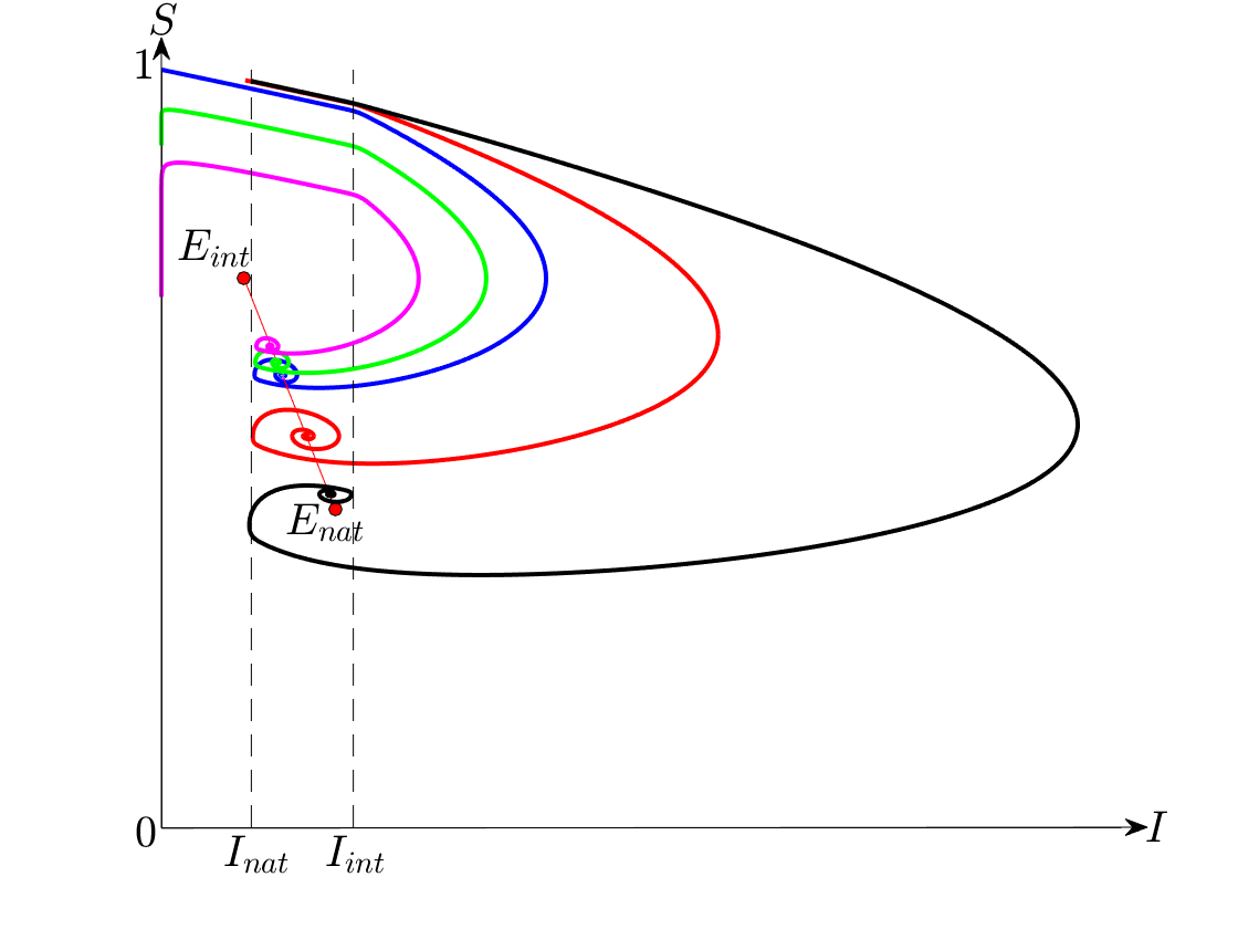
3.4. Let us consider a family of measure densities and the corresponding probability measures on depending on a parameter . Assume that these measures converge to a Dirac measure concentrated at a point as , i.e.
| (21) |
Let us denote the coordinates of the point by , and assume that they satisfy (6). Let be the line segment of equilibrium states of system (2) with the basic reproduction number given by
| (22) |
(cf. (17)).
Proposition 3
Let be the line segment of equilibrium states of system (2), (22). Let (21) hold where the coordinates of satisfy (6). Then, the following statements hold:
- –
if the line segment defined by (8) lies to the left of the line , then as ;
- –
if the line segment lies to the right of the line , then as ;
- –
if the line segment intersects the band , then as .
(a) (b)
(b)
This alternative can be compared to Proposition 1 describing the endemic equilibrium states of switched system (2), (7) depending on the relative position of points (8) and the thresholds lines . The proof is presented in Appendix 6.3.
3.5. We are now interested in the global maximum value of the infected population density along the trajectory of the epidemic. This quantity is important for estimating the maximum burden on the healthcare system. The trajectory of interest corresponds to the introduction of a small number of infected individuals into an entirely susceptible population, i.e. and .
(a) (b)
(b) (c)
(c) (d)
(d)  (e)
(e)  (f)
(f) 
Let us consider the ordinary differential system (2) where is a function of defined by
| (23) |
Denote by the unstable manifold of the saddle equilibrium of this system. That is, () is the heteroclinic trajectory connecting the infection free equilibrium with the positive stable equilibrium of system (2), (23). Assume that the equilibrium is a focus and denote by the first intersection point of the trajectory with the nullcline of system (2), (23). In other words,
Proposition 4

This proposition is used below to evaluate the maximum of numerically. The proof is presented in Appendix 6.4. As shown in the proof, is a trajectory of both the ordinary differential system (2), (23) and system (2), (17) with the Preisach operator; and, the endemic equilibrium of system (2), (23) coincides with the right end of the line segment of endemic equilibrium states of system (2), (17).
Typically, the recovery rate is much higher than the mortality rate , hence . In this case, (4) implies that the endemic equilibrium of system (2), (23) is a focus if the density is close to a -function. On the other hand, if is a node, then the heteroclinic trajectory converges to without crossing the nullcline , therefore . One can show that in this case trajectories of system (2), (17) with the Preisach operator satisfy
4 Discussion
A number of observations can be made from numerical simulations of the heterogeneous model (2), (17). As the density function in (17), we used the truncated Gaussian function
| (24) |
where is defined by the normalization condition (18). We observed the convergence to an endemic equilibrium state in all simulations. This is in contrast to switched system (2), (7) where certain threshold pairs lead to a periodic orbit (see Figure 2(abdf), 3). According to Proposition 2, a linear segment of endemic equilibrium states exists in the heterogeneous system. These endemic states differ by proportions of infected, susceptible and recovered individuals. The convergence upon the segment of endemic equilibrium states depends on the degree of heterogeneity of the public response (measured by the parameter ) and the threshold values at which the intervention is set to begin (the threshold ) and end (the threshold ). In particular, Figure 5(a) shows that if the intervention starts later, i.e. the threshold is higher, then the trajectory of the epidemic converges to an endemic state with higher proportions of infected and recovered individuals and a lower susceptible population. Revoking the intervention earlier, i.e. increasing the threshold , has a similar effect (see Figure 5(b)). This is to be expected. More interestingly, the same figures demonstrate that more heterogeneity in the public response tends to steer the epidemic towards an endemic equilibrium state with larger infected and recovered populations. However, there are exceptions to this general trend such as in Figure 6(e) where the infected population at the endemic equilibrium state depends on the degree of heterogeneity of the public response, , in a non-monotonic fashion. Further, we found that the maximum of the infected population along the epidemic trajectory demonstrates sensitive dependence on the heterogeneity parameter . Specifically, a higher heterogeneity of the public response leads to a higher peak of infection (see Figures 6, 7). These numerical results agree with, and complement, the statements of Propositions 2 – 4.
The density function of the Preisach operator can be estimated from simultaneous observations of and using the Mayergoyz identification theorem (Mayergoyz 2003). If increases from zero to a value , then drops back to zero, then increases to a value , the drops back to zero again, etc., and if the local maximum values of form an -net of the interval , then the identification theorem provides an -approximation of the density function from measurements of and . In the epidemiological context, this scenario corresponds to several waves of the epidemic. A number of practical identification algorithms can deal with measurement noise and limited amount of data, see e.g. Hoffmann et al., 1989; Cirrincione et al., 2002; Rachinskii et al., 2016. They include both non-parametric and parametric identification methods, where the latter assume a particular form of the density function such as in (24) or other (Appelbe et al., 2009; Krejčí et al., 2011; Krejčí et al., 2006; Brokate et al., 2011).
5 Conclusion
We considered an SIR model where the transmission coefficient changes in response to dynamics of the epidemic. We assumed that the adaptive response of an individual to the varying number of active cases can be modeled by a two-state two-threshold hysteretic switch. In an ideally homogeneous population, the two switching thresholds of the transmission coefficient can be imposed by the health authority which starts the intervention when the number of active cases exceeds a threshold and ends the intervention when the number of active cases drops below another threshold . In order to account for the possibility of a heterogeneous response among the susceptible individuals, we allowed a distribution of switching thresholds and modeled the aggregate response of the susceptible population by the Preisach operator. The mean of the distribution represents the thresholds and at which the health authority starts and ends the intervention; the variance of the distribution, , measures the degree of heterogeneity of the public response to the interventions. The resulting heterogeneous model is shown to have a continuum of endemic equilibrium states differing by the proportions of susceptible, infected and recovered populations.
Numerical simulations of the heterogeneous model provide an evidence that a wider spread of thresholds of different population groups leads to a significant increase of the peak of infection during the epidemic. Further, a higher degree of heterogeneity of the public response tends to steer the epidemic trajectory to an endemic equilibrium state with higher proportions of the infected and recovered populations and a lower proportion of the susceptible population. In other words, a more uniform response of the public to transmission prevention measures helps “flattening the curve” and can lead to smaller density of infection and lower when the endemic equilibrium state is reached after the epidemic. These results suggest that intervention programs are more effective when accompanied by education campaigns which convince the public to comply with the intervention policies. In particular, effective policy making should account for the culture and mindsets of the community when the intervention measures are decided upon, and the importance of these measures should be conveyed to the public to ensure a more homogeneous response.
The ideally homogeneous model predicts the lowest peak of infection. On the other hand, some threshold pairs lead to the convergence of the epidemic trajectory to a periodic orbit predicting recurrent outbreaks of the epidemic in a homogeneous population when its response is hysteretic. We observed that a slight degree of heterogeneity changes this scenario. The heterogeneous response ensures the convergence to an equilibrium state after a higher infection peak. These findings agree with the results of Kopfová et al. (2021) where the heterogeneity of the response was shown to promote the global stability of the set of endemic equilibrium states in an SIR model with vaccination. They are also associated with a trade-off between achieving the herd immunity faster with a higher infection peak or in a controlled manner but slower. Since expecting every member of the public to conform to the intervention policies exactly is unrealistic, some degree of heterogeneity with the associated effect on the epidemic dynamics can be assumed. The optimal choice of thresholds of the intervention policy is an interesting problem which extends beyond the scope of this paper. In reality, this choice is constraint by many factors such as the capacity of the healthcare system, the cost of the intervention measures to the economy and the willingness and readiness of the public to comply with intervention policies.
6 Appendix
6.1. Continuous Preisach model. Let us briefly recall a rigorous definition of the continuous Preisach operator (17) (Krasnosel’skii et al. 1983). It involves a collection of non-ideal relays , which respond to the same continuous input independently according to formula (11). The relays contributing to the system have different pairs of thresholds , where the subset of the half-plane is assumed to be measurable and bounded; the -plane is called the Preisach plane. The output of the continuous Preisach model is the scalar-valued function defined by (17), where is a positive bounded measurable function (measure density) representing the weights of the relays; and, is the initial state of the relay for any given . The function of the variable is referred to as the initial state function of the Preisach operator. It is assumed to be measurable and satisfy the constraints (9), (10), in which case the initial state-input pair is called compatible. These requirements ensure that the integral in (17) is well-defined for each and, furthermore, the output of the Preisach model is a continuous function of time. The function (11) with a fixed and varying is interpreted as the state function of the Preisach model at the moment as it describes the states of all the relays at this moment; this state function is an element of the space for each .
For brevity, let us denote the input-to-output operator of the Preisach model defined by (17) by
| (25) |
where both the input and the initial state function (which is compatible with the input) are the arguments; the value of this operator is the output . An important property of the Preisach operator (17) is that it is Lipschitz continuous if is bounded (Krasnosel’skii et al. 1983). More precisely, the relations
and () imply
| (26) |
for any with the Lipschitz constant
| (27) |
Let us denote by the set of all triplets , where and the initial state function of the Preisach operator is compatible with . The global Lipschitz estimate (26) ensures (for example, using the Picard-Lindelöf type of argument) that for a given , system (2) with the Preisach operator (17) has a unique local solution with the initial data and the initial state function (see, for example, the survey (Leonov 2017)). Further, the positive invariance of implies that each solution is extendable to the whole semi-axis . These solutions induce a continuous semi-flow in the set , which is considered to be the phase space of system (2), (17) and is endowed with a metric by the natural embedding into the space . This construction leads to the standard definition of local and global stability including stability of equilibrium states and periodic solutions. In particular, an equilibrium is a triplet and a periodic solution is a periodic function where the last component, viewed as a function of two variables and , is given by (12). The basic reproduction number (17) at an equilibrium is constant, while for a periodic solution the basic reproduction number changes periodically with the period of and .
6.2. Proof of Proposition 2. Consider the strictly decreasing functions (23) and
| (28) |
Due to the assumption and the normalization condition (18),
| (29) |
For every set
| (30) |
The constraint (10) implies that the basic reproduction number at an endemic equilibrium state equals for some . On the other hand, and are related to by formulas (3). Hence, is an endemic equilibrium state iff there is a such that
| (31) |
and
| (32) |
By definition, the positive function (30) is continuous in , strictly decreases in and strictly decreases in for . Therefore, the function
| (33) |
strictly increases in and . Since
equation (31) has a unique solution for each . By the Implicit Function Theorem, depends continuously on, and strictly decreases in, . Therefore, formulas (31), (32) imply that the endemic equilibrium states form a line segment on the -plane with and . Finally, from (29), (30) it follows that , hence from (31), (32) and (8) we conclude that , which completes the proof.
6.3. Proof of Proposition 3. Condition (21) implies that given any there is a such that for all the following relations hold:
| if | (34) | ||||
| if | (35) | ||||
| if | (36) | ||||
| if | (37) |
Without loss of generality, we assume that
| (38) |
Let us consider different cases of positioning he threshold .
Case 1: . In this case, set
and notice that implies due to (35). Therefore, the function (33) satisfies
| (39) |
because . On the other hand, since for all ,
| (40) |
Hence, a unique root of the equation satisfies , i.e.
| (41) |
Case 2: . Set , . Then,
as in (39). On the other hand,
and due to (34),
| (42) |
where the last inequality follows from (38). Therefore, the root of satisfies
| (43) |
Case 3: . In this case, set
and notice that implies due to (34). Therefore,
as in (42). On the other hand, since for all ,
hence , which is equivalent to
| (44) |
Since is arbitrarily small, relations (41), (43), (44) obtained in Cases 1 – 3, respectively, imply that the component of the equilibrium state satisfies
| (45) |
as . The same argument shows that relations (36), (37) imply a similar relationship
| (46) |
as for the equilibrium state . Relations (45), (46) are equivalent to the conclusion of the proposition.
6.4. Proof of Proposition 4. Consider the ordinary differential system (2) where :
| (47) | ||||
The positive equilibrium of this system coincides with the right end of the line segment of equilibrium states of system (2), (17).
Take an and denote . Denote by the trajectory of (47) starting at the point and continued in forward time. Let be sufficiently small to ensure that the point lies above the nullcline of system (47) defined by . By assumption, the positive equilibrium of (47) is a focus. Therefore, the trajectory intersects the nullcline . Denote by the first point of intersection of with the nullcline and by the arc of the curve , see Figure 8. Since above the nullcline , the curve is the graph of a continuous function :

The main step of the following proof is to show that a trajectory () of system (2), (17), which starts below the curve in the band with an arbitrary admissible initial state function of the Preisach operator, does not cross the line when continued in forward time. To this end, let us show that if , then the following implication holds:
| (48) |
Assume that there is a such that for . If we assume that , then on a sufficiently small time interval and hence
| (49) |
where the basic reproduction number is given by (17) with . But equations (13) and (17) imply that
| (50) |
| (51) |
at any time for any input and initial state function of the Preisach operator. In particular, at all times, hence
| (52) |
which is in contradiction with (49). This contradiction shows that . Since the initial point of the trajectory lies below the curve and the curve cannot cross the line segment due the positive invariance of the domain , from we conclude that and there is a such that
| (53) |
Next, let us consider the determinant
| (54) |
where the columns are the vector fields of systems (47) and (2), respectively. Notice that the segment , which belongs to the straight line , lies above the curve (because increases along this curve) and meets it at the point , see Figure 8. On this segment, with the exception of the point , the vector field of system (47) satisfies
Since the slope of the line segment is and the trajectory starts at the point above this segment, it follows that lies strictly above in the vertical band . Further, the line lies strictly below the curve for , and lies above this curve, hence lies strictly above the straight line for all . Therefore, (54) implies
| (55) |
on the curve , and from (50) it follows that on . On the other hand, the vector fields of systems (47) and (2) should satisfy the opposite inequality at the first intersection point of the trajectories and (cf. (53)) because the initial point of the trajectory lies to the left of the curve . Hence, at the first intersection point, which due to (50), (55) is equivalent to the relations
| (56) |
for the trajectory , where the basic reproduction number and the state function are given by equations (17) and (12) with .
The definitions (11) and (17) of the relay and the Preisach operator imply that is a trajectory of a solution () of system (2), (17) and that the basic reproduction number and the state function for this solution are defined by
| (57) |
on the interval . Due to the forward uniqueness property of solutions of system (2), (17), from (56), (57) it follows that the trajectories and of this system coincide after the moment when they merge, which completes the proof of the implication (48).
We conclude that if a trajectory starting below the curve in the band ever reaches the vertical line , then the intersection occurs at the point of the curve where , . Hence, crosses the line at the point vertically downwards to the domain where
due to (52). In other words, the point defined by (48) is an isolated point of local maximum for . Thus, the domain of the positive quadrant bounded form above by the curve and from the right by the vertical line (see Figure ) is invariant for system (2), (17) with any admissible initial state function of the Preisach operator:
In particular, any trajectory of (2), (17) starting in the -neighborhood of the point in the positively invariant domain satisfies
| (58) |
It remains to show that uniformly with respect to the initial condition and an admissible initial state function of the Preisach operator as . To this end, take such that
| (59) |
| (60) |
| (61) |
Take an and consider a trajectory of system (2), (17) satisfying . Notice that at the initial moment and due to (51), (59),
| (62) |
on some time interval . Further, as long as (62) holds, also and
which implies
Due to this estimate and (60), we conclude that the trajectory reaches the line before it reaches the line , i.e. there is a such that
Let us estimate the difference on the interval . From
after simple manipulations one obtains
where
Combining (62) and the similar estimates with (cf. (51)), and taking into account (61), we see that for , hence
and therefore
From (26), it follows that
where (respectively, ) is the state functions of the Preisach operator at the moment when for the trajectory (respectively, ). But the compatibility condition (13) implies that , hence
We see that the point of intersection of the trajectory with the line (which is independent of ) converges to the trajectory as , and the convergence is uniform with respect to the initial conditions from the set and all admissible initial states of the Preisach operator. Simultaneously, the state functions of the Preisach operator corresponding to for the trajectories and satisfy . Therefore, the continuous dependence of trajectories on the initial point in the phase space of system (2), (17) implies that the point of intersection of with the line converges to as for , which together with (58) proves the theorem.
References
- [1] Appelbe B, Flynn D, McNamara H, O’Kane P, Pimenov A, Pokrovskii A, Rachinskii D, Zhezherun A, 2009. Rate-independent hysteresis in terrestrial hydrology. IEEE Control Systems Magazine, 29(1): 44-69.
- [2] Brokate, M., Sprekels, J., 1996. Hysteresis and phase transitions, Vol. 121. Springer Science & Business Media. Springer-Verlag, NY.
- [3] M Brokate, S MacCarthy, A Pimenov, A Pokrovskii, D Rachinskii, 2011. Modelling energy dissipation due to soil-moisture hysteresis. Environmental Modeling & Assessment 16 (4), 313-333.
- [4] Chen, X., Fu, F., 2019. Imperfect vaccine and hysteresis, Proc. R. Soc. B 286 (1894), 20182406.
- [5] Center of Disease Control and Prevention (CDC), USA. 2021 Implementation of Mitigation Strategies for Communities with Local COVID-19 Transmission. https://www.cdc.gov/coronavirus/2019-ncov/community/community-mitigation.html (accessed 3 March 2021).
- [6] Chladná, Z., Kopfová, J., Rachinskii, D., Rouf, S., 2020. Global dynamics of SIR model with switched transmission rate. J. Math. Biology. 80, pp. 1209–1233.
- [7] Cirrincione M, Miceli R, Galluzzo GR, Trapanese M (2002) Preisach function identification by neural networks. IEEE Trans. Magn., 38(5): 2421-2423.
- [8] DeBenedetto, P., Ruiz, B., 2021. Houston Region Passes Threshold For Tougher COVID-19 Restrictions. https://www.houstonpublicmedia.org/articles/news/health-science/coronavirus/2021/01/05/388740/houston-area-projected-to-pass-governors-threshold-for-tougher-covid-19-restrictions-hidalgo-says/ (accessed 3 March 2021).
- [9] Department of Health and Human Services, Nebraska, 2020. Phased Public Health Restrictions Tied to Coronavirus Hospitalization Rate. https://dhhs.ne.gov/Documents/DHM-Measure-Table-ENGLISH.pdf (accessed 3 March 2021).
- [10] Emanuel, E.J., Persad, G., Upshur, R., Thome, B., Parker, M., Glickman, A., Zhang, C., Boyle, C., Smith, M., Phillips, J.P., 2020. Fair Allocation of Scarce Medical Resources in the Time of Covid-19. N Engl J Med. 382, pp. 2049-2055
- [11] Fairlie, R., 2020.The impact of COVID‐19 on small business owners: Evidence from the first three months after widespread social‐distancing restrictions. Journal of Economics and Management Strategy,29, 4, pp. 727-740.
- [12] Gostin, L.O., Wiley, L.F., 2020. Governmental Public Health Powers During the COVID-19 Pandemic: Stay-at-home Orders, Business Closures, and Travel Restrictions. JAMA. 323, 21, pp. 2137–2138.
- [13] Guidry, J. P. D., Laestadius, L. I., Vraga, E. K., Miller, C. A., Perrin, P. B., Burton, C. W., Ryan, M., Fuemmeler, B. F., Carlyle, K. E., 2021. Willingness to get the COVID-19 vaccine with and without emergency use authorization. American journal of infection control, 49, 2, pp. 137-142.
- [14] Hoffmann KH, Meyer GH (1989) A least squares method for finding the Preisach hysteresisoperator from measurements. Numer. Math., 55(6): 695-710.
- [15] Kopfová, J., Nábelková, P., Rachinskii, D., Rouf, S., 2021 Dynamics of SIR model with vaccination and heterogeneous behavioral response of individuals modeled by the Preisach operator. J. Math. Biology.
- [16] Krasnosel’skii, M.A., Pokrovskii, A.V., 1989. Static Hysteron. In Systems with Hysteresis. Springer, Berlin, Heidelberg. pp. 1-58.
- [17] Krejci, P., 1996. Hysteresis, convexity and dissipation in hyperbolic equations. Gakkotosho, Tokyo.
- [18] P Krejčí, JP O’Kane, A Pokrovskii, D Rachinskii, 2011. Stability results for a soil model with singular hysteretic hydrology. Journal of Physics: Conference Series 268 (1), 012016.
- [19] P Krejci, JP O’Kane, A Pokrovskii, D Rachinskii, 2006. Mathematical models of hydrological systems with Preisach hysteresis. BCRI Prepr. Ser 57, 1-46.
- [20] Marquioni, V. M., de Aguiar, M., 2020. Quantifying the effects of quarantine using an IBM SEIR model on scalefree networks. Chaos, solitons, and fractals, 138, 109999.
- [21] Matrajt, L., Leung, T., 2020. Evaluating the Effectiveness of Social Distancing Interventions to Delay or Flatten the Epidemic Curve of Coronavirus Disease. Emerging Infectious Diseases, 26, 8, pp. 1740-1748.
- [22] Mayergoyz, I.D., 2003. Mathematical Models of Hysteresis and Their Applications. Academic Press. New York, NY.
- [23] Lazarus, J.V., Ratzan, S.C., Palayew, A., 2021. A global survey of potential acceptance of a COVID-19 vaccine. Nat Med 27, pp. 225–228.
- [24] Leonov, G., Shumafov, M., Teshev, V., Aleksandrov, K., 2017. Differential equations with hysteresis operators. Existence of solutions, stability, and oscillations. Differ. Equ. 53, 13, pp. 1764-1816.
- [25] A Pimenov, TC Kelly, A Korobeinikov, MJA O’Callaghan, AV Pokrovskii, D Rachinskii, 2012. Memory effects in population dynamics: spread of infectious disease as a case study. Mathematical Modelling of Natural Phenomena 7, 3, pp. 204-226.
- [26] Rachinskii D, and Ruderman M. (2016) Convergence of direct recursive algorithm for identification of Preisach hysteresis model with stochastic input. SIAM Journal on Applied Mathematics, 76(4): 1270-1295.
- [27] Su, Z., Wang, W., Li, L., 2017. Emergence of hysteresis loop in social contagions on complex networks. Sci Rep 7, 6103.
- [28] Visintin, A., 2006. Mathematical Models of Hysteresis., in: Mayergoyz, I.D., Bertotti, G. (Eds.), The Science of Hysteresis. Elsevier, pp. 1-123.
- [29] Wilder-Smith, A., Chiew, C.J., Lee, V.J., 2020. Can we contain the COVID-19 outbreak with the same measures as for SARS? Lancet Infect Dis. 20, 5. pp. e102-e107.