跳到论文正文
W Papers独立论文阅读器 arXiv:2103.07979 论文正文 计算阅读时间 · 0%
引用这篇论文根据当前论文元数据生成,正式投稿前建议核对。


License: CC Zero
arXiv:2103.07979v1 [hep-th] 14 Mar 2021

Influence of the four-fermion interactions in (2+1)D massive electrons system

Luis Fernández Email: luis.aguilar@icen.ufpa.br Affiliation: Faculdade de Física, Universidade Federal do Pará, 66075-110 Belém, Pará, Brazil    Van Sérgio Alves Email: vansergi@ufpa.br Affiliation: Faculdade de Física, Universidade Federal do Pará, 66075-110 Belém, Pará, Brazil    M. Gomes Email: mgomes@fma.if.usp.br Affiliation: Instituto de Física, Universidade de São Paulo, Caixa Postal 66318, 05315-970 São Paulo, São Paulo, Brazil    Leandro O. Nascimento Email: lon@ufpa.br Affiliation: Faculdade de Ciências Naturais, Universidade Federal do Pará, C.P. 69900-000 Breves, Pará, Brazil    Francisco Peña Email: francisco.pena@ufrontera.cl Affiliation: Departamento de Ciencias Físicas, Facultad de Ingeniería y Ciencias, Univesidad de La Frontera, Avenida Francisco Salazar 01145, Casilla 54-D, Temuco, Chile
August 11, 2026
Abstract

The description of the electromagnetic interaction in two-dimensional Dirac materials, such as graphene and transition-metal dichalcogenides, in which electrons move in the plane and interact via virtual photons in 3d, leads naturally to the emergence of a projected non-local theory, called pseudo-quantum electrodynamics (PQED), as an effective model suitable for describing electromagnetic interaction in these systems. In this work, we investigate the role of a complete set of four-fermion interactions in the renormalization group functions when we coupled it with the anisotropic version of massive PQED, where we take into account the fact that the Fermi velocity is not equal to the light velocity. We calculate the electron self-energy in the dominant order in the 1/N1/N expansion in the regime where m2≪p2m^{2}\ll p^{2}. We show that the Fermi velocity renormalization is insensitive to the presence of quartic fermionic interactions, whereas the renormalized mass may have two different asymptotic behaviors at the high-density limit, which means a high-energy scale.

I INTRODUCTION

Four-fermion interactions have been extensively studied in the literature, both for understanding conceptual aspects of quantum field theory as well as for applications in condensed matter physics. In particular, the Thirring Thirring and Nambu-Jona-Lasinio NJL models show a rich connection between the phenomenon of superconductivity and elementary particle physics. The latter has also been used for studying quantum chromodynamics at the low-energy limit Cahil; Hatsuda. Although four-fermion interactions are perturbatively non-renormalizable in a space-time D>2D>2, in the sense of general power counting rules Dyson, they become renormalizable when we use the 1/N1/N expansion in D=3D=3 four1/N. Indeed, the incorporation of vacuum polarization effects provide a better behavior for the Green functions in the ultraviolet regime. Therefore, both the Gross-Neveu GN and Thirring MGomes interactions may be renormalizable in D=3D=3. Usually, in order to perform the 1/N1/N expansion, it is used a Hubbard-Stratonovich transformation hubbard through the introduction of an auxiliary field, which has no dynamics at the tree level.

It is well known that the quasiparticle excitations in two-dimensional materials at the honeycomb lattice (such as graphene Grafeno, silicene Siliceno, and transition metal dichalcogenides TMD) behave as Dirac-like fermions (either massless or massive). Hence, the four-fermion interactions also become relevant, as an attempt to obtain a more complete description of these systems, within a quantum-field-theory approach. Indeed, this more realistic description should take into account some of the microscopic interactions that, such as disorder/impurity, may emerge in these materials. Because the auxiliary fields obey the same properties as the random disorder/impurities interactions, as discussed in Refs.Liu; Wang, hence, we can relate these properties of the materials with the four-fermion interactions, within the low-energy limit. Furthermore, it is also very useful to consider the electromagnetic interactions in the plane, which may be effectively described by the pseudo-quantum electrodynamics model marino.

In a previous work we analyzed the effect of the electromagnetic interaction on the renormalization of the mass gap of electrons moving in a plane subject also to impurities simulated by a Gross-Neveu like self-interaction fernandez. Without the four-fermion interaction, we derived results that are in excellent agreement with experimental measurements of the band gap for WSe2 WSe and MoS2 MoS. We found also that, although the presence of the Gross-Neveu like interaction does not alter the renormalization of the Fermi velocity vozmediano, it provides an ultraviolet fixed point in terms of an effective fine-structure constant, so that the renormalized mass has different behaviors below and above it.

In this paper we extend the investigation presented in fernandez by considering the generalized four-fermion interactions with O⁡(4)O(4) symmetry.

The remainder of this paper is organized as follow. In Sec. II we present our model, notation, and perform the expansion 1/N1/N through the Hubbard-Stratonovich transformation, which allow us to define the Feynman rules. In Sec. III we calculate the propagators of the gauge and auxiliary fields in the dominant order in 1/N1/N in the regime where m2≪p2m^{2}\ll p^{2}. In Sec. IV we calculate the electron self-energy due to electromagnetic and the four-fermions interactions, taking into account the effect of the polarization tensor obtained in the previous section. The derivation of the renormalization group functions and the effect of each four-fermion interaction on the renormalized mass are shown in Sec.V. In Sec. VI we review our main results and conclusions. Some details about the derivation of the polarization tensor, due to the four-fermion interactions, are given in Appendix A.

II PSUEDO-QUANTUM ELECTRODYNAMICS WITH FOUR-FERMIONS INTERACTION

We consider the PQED model marino with a complete set of independent four-fermion interactions in (2+1)D gomes1. The Euclidean action reads

ℒ=12​Fμ​ν​Fμ​ν−□+ψ¯a​(ı˙​γμ​Dμ−m)​ψa−ξ​(∂μAμ)2−□−∑8l=1Gl2(ψ¯aΓlψa)2,\begin{split}\mathcal{L}&=\frac{1}{2}\frac{F^{\mu\nu}F_{\mu\nu}}{\sqrt{-\Box}}+\bar{\psi}_{a}\left(\dot{\imath}\gamma^{\mu}D_{\mu}-m\right)\psi_{a}-\xi\frac{\left(\partial_{\mu}A^{\mu}\right)^{2}}{\sqrt{-\Box}}\\ &-\sum^{8}_{l=1}\frac{G_{l}}{2}\left(\bar{\psi}_{a}\Gamma^{l}\psi_{a}\right)^{2},\end{split} (1)

where Fμ​ν=∂μAν−∂νAμF_{\mu\nu}=\partial_{\mu}A_{\nu}-\partial_{\nu}A_{\mu} is the field intensity tensor of the gauge field AμA_{\mu}, □\Box is the d’Alembertian operator, ψa\psi_{a} is the Dirac field, and a=1,…,Na=1,...,N is the flavor index. For electrons in the honeycomb lattice, we may use the representation for matter field as ψa†=(ψA↑∗,ψA↓∗,ψB↑∗,ψB↓∗)a\psi_{a}^{\dagger}=(\psi^{*}_{A\uparrow},\psi^{*}_{A\downarrow},\psi^{*}_{B\uparrow},\psi^{*}_{B\downarrow})_{a}, where (A,B)(A,B) and (↑,↓)(\uparrow,\downarrow) are the sublattices and spins, respectively. Therefore, one finds a=K,K′a=K,K^{\prime} and N=2N=2 that describes the valley degeneracy. Here, we perform all of the calculations for an arbitrary value of NN Gfactor; libroMarino. Furthermore, mm is the Dirac mass, ee is the electric charge, ξ\xi is the gauge-fixing parameter, Gl={G1,…,G8}G_{l}=\{G_{1},...,G_{8}\} are the coupling constants of the four-fermion interactions where l=1,…,8l=1,...,8 is an index describing each self-interaction, Γl={𝟙,γμ,γ3,γ5,γμ​γ3,γμ​γ5,γ3​γ5,γμ​γ3​γ5}\Gamma_{l}=\{\mathbbm{1},\gamma^{\mu},\gamma^{3},\gamma^{5},\gamma^{\mu}\gamma^{3},\gamma^{\mu}\gamma^{5},\gamma^{3}\gamma^{5},\gamma^{\mu}\gamma^{3}\gamma^{5}\} are their corresponding matrices, γμ\gamma^{\mu} are the Dirac matrices in the 4×44\times 4 representation, whose algebra is given by {γμ,γν}=−2​δμ​ν\left\{\gamma^{\mu},\gamma^{\nu}\right\}=-2\delta^{\mu\nu}, and γμ​Dμ\gamma^{\mu}D_{\mu}=γ0∂0+vFγi∂i+eγμAμ\gamma^{0}\partial_{0}+v_{F}\gamma^{i}\partial_{i}+e\gamma^{\mu}A_{\mu} is the Dirac operator after we perform the minimal coupling with AμA_{\mu}. Our matrix representation follows the definition given in Ref. wang. Thus, our Dirac matrices are anti-hermitian: (γ0,γ1,γ2)=(iσ3,iσ1,iσ2)⊗,σ3),γ3=I⊗σ1(\gamma_{0},\gamma_{1},\gamma_{2})=(i\sigma_{3},i\sigma_{1},i\sigma_{2})\otimes,\sigma_{3}),\gamma_{3}=I\otimes\sigma_{1} and γ5≡I⊗σ2\gamma_{5}\equiv I\otimes\sigma_{2} so that (γμ)2=−1(\gamma_{\mu})^{2}=-1, and γ5\gamma_{5} is Hermitian. Furthermore, we shall use the natural system of units, where ℏ=c=1\hbar=c=1. Because [Gl]=−1[G_{l}]=-1, the model in Eq. (1) is not renormalizable in the perturbative expansion, but it is in the large-NN expansion. Hence, we shall consider the large-NN expansion from now on.

The first step is to introduce the NN parameter into the action through a scaling of the coupling constants, given by e→e/Ne\rightarrow e/\sqrt{N} and Gl→Gl/NG_{l}\rightarrow G_{l}/N for a fixed ee and GlG_{l}, respectively. Thereafter, we use a Hubbard-Stratonovich transform in the four-fermion interactions, given by

Gl2​N​(ψ¯a​Γl​ψa)2→Gl2​N​(ψ¯a​Γl​ψa)2−N2​G1​[φ1−G1N​ψ¯a​Γ1​ψa]2−…−N2​G8​[φ8−G8N​ψ¯a​Γ8​ψa]2,\begin{split}\frac{G_{l}}{2N}\left(\bar{\psi}_{a}\Gamma^{l}\psi_{a}\right)^{2}&\rightarrow\frac{G_{l}}{2N}\left(\bar{\psi}_{a}\Gamma^{l}\psi_{a}\right)^{2}\\ &-\frac{N}{2G_{1}}\left[\varphi_{1}-\frac{G_{1}}{N}\bar{\psi}_{a}\Gamma_{1}\psi_{a}\right]^{2}-...\\ &-\frac{N}{2G_{8}}\left[\varphi_{8}-\frac{G_{8}}{N}\bar{\psi}_{a}\Gamma_{8}\psi_{a}\right]^{2},\end{split} (2)

where

φl={φ𝟙,φγμ,φγ3,φγ5,φγμ​γ3,φγμ​γ5,φγ3​γ5,φγμ​γ3​γ5}\varphi_{l}=\{\varphi_{\mathbbm{1}},\varphi_{\gamma^{\mu}},\varphi_{\gamma^{3}},\varphi_{\gamma^{5}},\varphi_{\gamma^{\mu}\gamma^{3}},\varphi_{\gamma^{\mu}\gamma^{5}},\varphi_{\gamma^{3}\gamma^{5}},\varphi_{\gamma^{\mu}\gamma^{3}\gamma^{5}}\}

is a set of auxiliary fields for each kind of interaction. Note that, for the sake of simplicity, we applied the notation φl={φ1,…,φ8}\varphi_{l}=\{\varphi_{1},...,\varphi_{8}\} in Eq. (2). Using Eq. (2) in Eq. (1), one finds the motion equation for the auxiliary fields, namely, φl=Gl​ψ¯a​Γl​ψa/N\varphi_{l}=G_{l}\bar{\psi}_{a}\Gamma_{l}\psi_{a}/N at classical level for each l=1,…,8l=1,...,8 (there is no sum over ll in the rhs of this equation). Furthermore, we also obtain the action

ℒ=12Fμ​ν​Fμ​ν−□+ψ¯(ı˙γ0∂0+ı˙vFγi∂i−m)ψ++eN​ψ¯​γμ​ψ​Aμ−ξ​(∂μAμ)2−□+∑8l=1[N2​Glφl2−φlψ¯Γlψ].\begin{split}\mathcal{L}&=\frac{1}{2}\frac{F^{\mu\nu}F_{\mu\nu}}{\sqrt{-\Box}}+\bar{\psi}\left(\dot{\imath}\gamma^{0}\partial_{0}+\dot{\imath}v_{F}\gamma^{i}\partial_{i}-m\right)\psi+\\ &+\frac{e}{\sqrt{N}}\bar{\psi}\gamma^{\mu}\psi A_{\mu}-\xi\frac{\left(\partial_{\mu}A^{\mu}\right)^{2}}{\sqrt{-\Box}}\\ &+\sum^{8}_{l=1}\left[\frac{N}{2G_{l}}\varphi_{l}^{2}-\varphi_{l}\bar{\psi}\Gamma_{l}\psi\right].\end{split} (3)

Next, we realize a simple shift in the auxiliary field, namely, φl→σ0,l+φl/N\varphi_{l}\rightarrow\sigma_{0,l}+\varphi_{l}/\sqrt{N} such that σ0,l=⟨φl⟩\sigma_{0,l}=\braket{\varphi_{l}} is the vacuum expectation value of φl\varphi_{l}. Using this transform in Eq. (3), we have

ℒ=12Fμ​ν​Fμ​ν−□+ψ¯(ı˙γ0∂0+ı˙vFγi∂i−m−σ0,lΓl)ψ+eN​ψ¯​γμ​ψ​Aμ−ξ​(∂μAμ)2−□+∑l=18[N2​Gl​σ0,l2]+∑8l=1[12​Glφl2−NGlσ0,lφl−1Nφlψ¯Γlψ].\begin{split}\mathcal{L}&=\frac{1}{2}\frac{F^{\mu\nu}F_{\mu\nu}}{\sqrt{-\Box}}\!+\!\bar{\psi}\left(\dot{\imath}\gamma^{0}\partial_{0}\!+\!\dot{\imath}v_{F}\gamma^{i}\partial_{i}-m\!-\!\sigma_{0,l}\Gamma_{l}\right)\!\psi\\ &+\frac{e}{\sqrt{N}}\bar{\psi}\gamma^{\mu}\psi A_{\mu}-\xi\frac{\left(\partial_{\mu}A^{\mu}\right)^{2}}{\sqrt{-\Box}}+\sum^{8}_{l=1}\left[\frac{N}{2G_{l}}\sigma_{0,l}^{2}\right]\\ &+\sum^{8}_{l=1}\left[\frac{1}{2G_{l}}\varphi_{l}^{2}-\frac{\sqrt{N}}{G_{l}}\sigma_{0,l}\varphi_{l}-\frac{1}{\sqrt{N}}\varphi_{l}\bar{\psi}\Gamma_{l}\psi\right].\end{split} (4)

One advantage of Eq. (4) is that for m=0m=0 it clearly separates the analysis into phases, i.e, one with no spontaneous symmetry breaking where σ0,l=0\sigma_{0,l}=0 and other phases with some broken symmetry σ0,l≠0\sigma_{0,l}\neq 0. In particular, a phase with chiral symmetry breaking , i.e, σ0,1≠0\sigma_{0,1}\neq 0 has been discussed in Ref. fernandez. Next, let us define the Feynman rules. The gauge-field propagator in Eq. (3) reads

Δμ​ν0​(p)=12​p​[δμ​ν−(1−1ξ)​pμ​pνp2],\Delta^{0}_{\mu\nu}(p)=\frac{1}{2\sqrt{p}}\left[\delta_{\mu\nu}-\left(1-\frac{1}{\xi}\right)\frac{p_{\mu}p_{\nu}}{p^{2}}\right], (5)

while the fermion propagator is given by

SF​(p)=−1γ0​p0+vF​γi​pi−m,S_{F}(p)=-\frac{1}{\gamma^{0}p_{0}+v_{F}\gamma^{i}p_{i}-m}, (6)

and,in the tree approximation, the propagator for the auxiliary-field φl\varphi_{l} is

(Δφl0)=(1Gl)−1.\left(\Delta^{0}_{{\varphi_{l}}}\right)=\left(\frac{1}{G_{l}}\right)^{-1}. (7)

The electromagnetic and trilinear vertices interactions are given by e/Ne/\sqrt{N} and 1/N1/\sqrt{N}, respectively. Next, we shall calculate the quantum corrections, within the large-NN approximation, for the field propagators.

III FULL PROPAGATORS

III.1 Gauge-field propagator

The full gauge-field propagator, in the dominant order of 1/N1/N, is written as fernandez

Δμ​ν​(p)=Δμ​ν0​(p)+Δμ​α0​(p)​Πα​β​(p)​Δβ​ν0​(p)+⋯,\Delta_{\mu\nu}(p)=\Delta_{\mu\nu}^{0}(p)+\Delta_{\mu\alpha}^{0}(p)\Pi^{\alpha\beta}(p)\Delta_{\beta\nu}^{0}(p)+\cdots, (8)

where Πμ​ν​(p)\Pi^{\mu\nu}(p) is the vacuum polarization tensor, namely,

Πμ​ν(p)=−e2NTr∫d3​k(2​π)3γμSF(p+k)γνSF(k).\Pi^{\mu\nu}(p)=-\frac{e^{2}}{N}{\rm Tr}\int\frac{d^{3}k}{(2\pi)^{3}}\gamma^{\mu}S_{F}(p+k)\gamma^{\nu}S_{F}(k). (9)

In the static limit, we only need the component Π00​(p)\Pi^{00}(p) given by

Π00​(p2)=−e28​p2p02+vF2​p2\Pi^{00}(\textbf{p}^{2})=-\frac{e^{2}}{8}\frac{\textbf{p}^{2}}{\sqrt{p_{0}^{2}+v_{F}^{2}\textbf{p}^{2}}} (10)

in the small-mass limit m2≪p2m^{2}\ll p^{2}. Using Eq. (10) in Eq. (8), we find

Δ00​(p2)=(2​p2+e28​p2p02+vF2​p2)−1.\Delta_{00}(\textbf{p}^{2})=\left(2\sqrt{\textbf{p}^{2}}+\frac{e^{2}}{8}\frac{\textbf{p}^{2}}{\sqrt{p_{0}^{2}+v_{F}^{2}\textbf{p}^{2}}}\right)^{-1}. (11)

This agrees with the result in Ref. fernandez.

III.2 Auxiliary-field propagators

The quantum corrections for the auxiliary fields φl\varphi_{l} may be obtained through the effective action SeffS_{\rm eff}. This is accomplished from Eq. (4) by integrating out the matter field. After expanding SeffS_{\rm eff} for large-NN, we find

Seff​[φl]=N​S1​[φl]+S2​[φl]+⋯,S_{\rm eff}[\varphi_{l}]=\sqrt{N}S_{1}[\varphi_{l}]+S_{2}[\varphi_{l}]+\cdots, (12)

where

S1=Tr[(ı˙γ0∂0+ı˙vFγi∂i−m−σo,lΓl)−1×(∑lφlΓl)]+∑l1Glσ0,lφl\begin{split}S_{1}&={\rm Tr}\left[\left(\dot{\imath}\gamma^{0}\partial_{0}+\dot{\imath}v_{F}\gamma^{i}\partial_{i}-m-\sigma_{o,l}\Gamma^{l}\right)^{-1}\right.\\ &\left.\times\left(\sum_{l}\varphi_{l}\Gamma^{l}\right)\right]+\sum_{l}\frac{1}{G_{l}}\sigma_{0,l}\varphi_{l}\end{split} (13)

and

S2=12Tr[{(ı˙γ0∂0+ı˙vFγi∂i−m−σo,lΓl)−1×(∑lφlΓl)}2]+∫d3x∑l12​Glφl2.\begin{split}S_{2}&=\frac{1}{2}{\rm Tr}\left[\left\{\left(\dot{\imath}\gamma^{0}\partial_{0}+\dot{\imath}v_{F}\gamma^{i}\partial_{i}-m-\sigma_{o,l}\Gamma^{l}\right)^{-1}\right.\right.\\ &\left.\left.\times\left(\sum_{l}\varphi_{l}\Gamma^{l}\right)\right\}^{2}\right]+\int d^{3}x\sum_{l}\frac{1}{2G_{l}}\varphi_{l}^{2}.\end{split} (14)

Note that S1S_{1} in Eq. (13) may be written as S1=∑lφl​Sl​[σ0,l,Gl]S_{1}=\sum_{l}\varphi_{l}S_{l}[\sigma_{0,l},G_{l}]. On the other hand, we have that S1=0S_{1}=0 which implies a convergent effective action in Eq. (12). This yields a set of gap equations Sl​[σ0,l,Gl]=0S_{l}[\sigma_{0,l},G_{l}]=0 for each ll, giving a nontrivial relation between the values of σ0,l\sigma_{0,l} and the coupling constants GlG_{l}. However, for σ0,l=0\sigma_{0,l}=0 and m=0m=0 these gap equations are automatically satisfied.

Next, it is convenient to write Eq. (14) as

S2=12​∫d3​x​d3​y​φl​(x)​Γl​l′​(x−y)​φl′​(y),S_{2}=\frac{1}{2}\int d^{3}x\,d^{3}y\,\,\varphi_{l}(x)\,\Gamma^{ll^{\prime}}(x-y)\,\varphi_{l^{\prime}}(y), (15)

providing the auxiliary-field propagator Γl​l′​(x−y)−1\Gamma^{ll^{\prime}}(x-y)^{-1}. This, in the momentum space, is schematically written as

[Δ{φl}l​l′​(p)]−1=Γ{φl}l​l′​(p)=1G{φl}​δl​l′−Π{φl}l​l′​(p).\left[\Delta^{ll^{\prime}}_{\{\varphi_{l}\}}(p)\right]^{-1}=\Gamma^{ll^{\prime}}_{\{\varphi_{l}\}}(p)=\frac{1}{G_{\{\varphi_{l}\}}}\delta^{ll^{\prime}}-\Pi^{ll^{\prime}}_{\{\varphi_{l}\}}(p). (16)

At this point, we must be careful with our notation in order to avoid any misunderstanding. Indeed, the kind of indexes (l​l′)(ll^{\prime}) we have in Eq. (16) depends on the kind of auxiliary field {φl}\{\varphi_{l}\} we want to consider. For instance, φ1=φ𝟙→σ\varphi_{1}=\varphi_{\mathbbm{1}}\rightarrow\sigma is a scalar field, hence, δl​l′\delta^{ll^{\prime}} only means an unity. Nevertheless, we may consider the second auxiliary field, which is actually φ2=φγμ→𝒜μ\varphi_{2}=\varphi_{\gamma_{\mu}}\rightarrow{\cal A}_{\mu} a vector field. In this case, we must consider that δl​l′→δμ​ν\delta^{ll^{\prime}}\rightarrow\delta^{\mu\nu}, where we replace (l​l′)(ll^{\prime}) by two Lorentz indexes, i.e, (l​l′)→(μ​ν)(ll^{\prime})\rightarrow(\mu\nu), such that we find a propagator Δ{φμ}μ​ν​(p)\Delta^{\mu\nu}_{\{\varphi_{\mu}\}}(p), as expected. The main rule is that for a generic auxiliary field {φl}\{\varphi_{l}\}, one must have a scalar quantity S2∝φl​Γl​l′​φl′S_{2}\propto\varphi_{l}\Gamma^{ll^{\prime}}\varphi_{l^{\prime}}, which, therefore, fixes the tensorial structure of Γl​l′\Gamma^{ll^{\prime}}. We represent the full propagator of the auxiliary fields in Fig. 1.

Refer to caption
Figure 1: The large-NN approximation for the full auxiliary-field propagators. The full propagators of the auxiliary fields are represented by the double-dashed line with the subscripts (l,l′)(l,l^{\prime}), which are meant to describe their different tensorial structure. The continuum line is the propagator of the fermion field.

The different self-energies for each auxiliary field read

Π{φl}l​l′(p)=−Tr∫d3​k(2​π)3ΓlSF(p+k)Γl′SF(k).\Pi^{ll^{\prime}}_{\{\varphi_{l}\}}(p)=-{\rm Tr}\int\frac{d^{3}k}{(2\pi)^{3}}\Gamma^{l}S_{F}(p+k)\Gamma^{l^{\prime}}S_{F}(k). (17)

We consider the 4×44\times 4 representation of the Dirac matrices, whose trace operations are detailed in appendix A. Because of the Lorentz symmetry in the Dirac matrices, we perform a redefinition of the external momentum as vF​pi→p¯iv_{F}p_{i}\rightarrow\bar{p}_{i}, such that p¯μ=(p0,p¯i)\bar{p}_{\mu}=(p_{0},\bar{p}_{i}). Furthermore, for the sake of consistency, we also change the spatial-variable of the loop integral as vF​ki→kiv_{F}k_{i}\rightarrow k_{i}, which implies that d3​k→d3​k/vF2d^{3}k\rightarrow d^{3}k/v_{F}^{2}. Therefore,

Π{φl}l​l′(p¯)=−1vF2Tr∫d3​k(2​π)3ΓlSF(p¯+k)Γl′SF(k).\Pi^{ll^{\prime}}_{\{\varphi_{l}\}}(\bar{p})=-\frac{1}{v_{F}^{2}}{\rm Tr}\int\frac{d^{3}k}{(2\pi)^{3}}\Gamma^{l}S_{F}(\bar{p}+k)\Gamma^{l^{\prime}}S_{F}(k). (18)

It is clear that the only difference, between the different four-fermion interactions, is the vertex structure Γl\Gamma_{l} (and Γl′\Gamma_{l^{\prime}}) in Eq. (18).

IV The Electron Self-Energy

We assume the symmetric phase, where σ0,l=0\sigma_{0,l}=0. This phase is promptly obtained from Eq. (4) by using σ0,l=0\sigma_{0,l}=0. Using the Feynman parametrization and the dimensional regularization (See Appendix A), we obtain the self-energies for all of the auxiliary fields φl\varphi_{l} which for higher momenta, is given by

Γφ𝟙​(p¯)\displaystyle\Gamma_{\varphi_{\mathbbm{1}}}(\bar{p}) =1Gφ𝟙+p¯24​vF2,\displaystyle=\frac{1}{G_{\varphi_{\mathbbm{1}}}}+\frac{\sqrt{\bar{p}^{2}}}{4v_{F}^{2}}, (19)
Γφμμ​ν​(p¯)\displaystyle\Gamma_{\varphi_{\mu}}^{\mu\nu}(\bar{p}) =(1Gφμ+p¯28​vF2)​ℙ¯μ​ν+1Gφμ​p¯μ​p¯νp¯2,\displaystyle=\left(\frac{1}{G_{\varphi_{\mu}}}+\frac{\sqrt{\bar{p}^{2}}}{8v_{F}^{2}}\right)\mathbb{\bar{P}}^{\mu\nu}+\frac{1}{G_{\varphi_{\mu}}}\frac{\bar{p}^{\mu}\bar{p}^{\nu}}{\bar{p}^{2}}, (20)
Γφ3​(5)​(p¯)\displaystyle\Gamma_{\varphi_{3(5)}}(\bar{p}) =1Gφ3​(5)−p¯24​vF2,\displaystyle=\frac{1}{G_{\varphi_{3(5)}}}-\frac{\sqrt{\bar{p}^{2}}}{4v_{F}^{2}}, (21)
Γφμ​3​(5)μ​ν​(p¯)\displaystyle\Gamma^{\mu\nu}_{\varphi_{\mu 3(5)}}(\bar{p}) =(1Gφμ​3​(5)+p¯28​vF2)​ℙ¯μ​ν+1Gφμ​3​(5)​p¯μ​p¯νp¯2,\displaystyle=\!\!\left(\!\frac{1}{G_{\varphi_{\mu 3(5)}}}\!+\!\frac{\sqrt{\bar{p}^{2}}}{8v_{F}^{2}}\right)\mathbb{\bar{P}}^{\mu\nu}+\frac{1}{G_{\varphi_{\mu 3(5)}}}\frac{\bar{p}^{\mu}\bar{p}^{\nu}}{\bar{p}^{2}}, (22)
Γφ35​(p¯)\displaystyle\Gamma_{\varphi_{35}}(\bar{p}) =1Gφ35+p¯24​vF2,\displaystyle=\frac{1}{G_{\varphi_{35}}}+\frac{\sqrt{\bar{p}^{2}}}{4v_{F}^{2}}, (23)

and

Γφμ​35μ​ν​(p¯)=(1Gφμ​35−p¯28​vF2)​ℙ¯μ​ν+1Gφμ​35​p¯μ​p¯νp¯2.\Gamma^{\mu\nu}_{\varphi_{\mu 35}}(\bar{p})=\!\!\left(\!\frac{1}{G_{\varphi_{\mu 35}}}\!-\!\frac{\sqrt{\bar{p}^{2}}}{8v_{F}^{2}}\right)\mathbb{\bar{P}}^{\mu\nu}+\frac{1}{G_{\varphi_{\mu 35}}}\frac{\bar{p}^{\mu}\bar{p}^{\nu}}{\bar{p}^{2}}. (24)

The subscription 3​(5)3(5) means that the result holds for both φ3\varphi_{3} and φ5\varphi_{5} fields, for example. Furthermore, the standard projection tensor ℙ¯μ​ν\mathbb{\bar{P}}^{\mu\nu} reads

ℙ¯μ​ν=δμ​ν−p¯μ​p¯νp¯2.\mathbb{\bar{P}}^{\mu\nu}=\delta^{\mu\nu}-\frac{\bar{p}^{\mu}\bar{p}^{\nu}}{\bar{p}^{2}}. (25)

It should be noticed the bad ultraviolet behavior of the longitudinal part of the two point proper function involving a vectorial field, namely the longitudinal parts in Eqs. (20), (22), and (24). Of course, these bad behaviors are innocuous if the corresponding currents are conserved. In any case, this fact is only relevant for calculating the correction in order 1/N21/N^{2}. If we consider only the transversal part of these propagators, the generalized model (3) is power counting renormalizable with divergences being eliminated by reparametrizations of the fields and of the mass of the fermion field. In what follows we will discuss in detail the divergences in the fermion self-energy.

IV.1 The Fermion Self-enegy

Having the gauge and auxiliary-field propagators, we may calculate the fermion self-energy. This also may be decomposed into two terms, one due to the gauge field and the other due to the auxiliary fields.

Refer to caption
Figure 2: The full fermion propagator up to the dominant order 1/N1/N. The full fermion propagator is represented by the double continuos lines. OPENa)a) The self-energy due to the interaction between the gauge and fermion fields. OPENb)b) The general structure of the self-energies due to each auxiliary-field propagator and the fermion field.

IV.1.1 Self-energy due to the gauge field

The fermion self-energy due to the gauge field is shown in Fig 2.a and its analytical expression is given by

ΣAμ​(p)=e2N​∫d3​k(2​π)3​γμ​SF​(p−k)​γν​Δμ​ν​(k).\Sigma_{A_{\mu}}(p)=\frac{e^{2}}{N}\int\frac{d^{3}k}{(2\pi)^{3}}\gamma^{\mu}S_{F}(p-k)\gamma^{\nu}\Delta_{\mu\nu}(k). (26)

The first step is to use Eq. (6) and Eq. (11) in Eq. (26). On the other hand, the self-energy in the small-momentum limit, which is the revelant term in order to extract the form of the divergences, is written as fernandez; son

ΣAμ​(p)=ΣAμ​(p)|p=0+γ0​p0​∂ΣAμ​(p0)∂p0|p0=0+vF​γi​pi​∂ΣAμ​(pi)∂pi|pi=0+⋯.\begin{split}\Sigma_{A_{\mu}}(p)&=\Sigma_{A_{\mu}}(p)\Bigm|_{p=0}+\gamma^{0}p_{0}\frac{\partial\Sigma_{A_{\mu}}(p_{0})}{\partial p_{0}}\Bigm|_{p_{0}=0}\\ &+v_{F}\gamma^{i}p_{i}\frac{\partial\Sigma_{A_{\mu}}(p_{i})}{\partial p_{i}}\Bigm|_{p_{i}=0}+\cdots.\end{split} (27)

After some calculations, (see App. A of ref. fernandez) it is possible to show that the fermion self-energy, in the small-mass limit, is

ΣAμ​(p)=−2​λπ2​N[γ0p0f1(λ)−vFγipif2(λ)+mf0(λ)]ln(ΛΛ0)+FT,\begin{split}\Sigma_{A_{\mu}}(p)&=-\frac{2\lambda}{\pi^{2}N}\left[\gamma^{0}p_{0}f_{1}(\lambda)-v_{F}\gamma^{i}p_{i}f_{2}(\lambda)\right.\\ &\left.+mf_{0}(\lambda)\right]\ln\left(\frac{\Lambda}{\Lambda_{0}}\right)+\textrm{FT},\end{split} (28)

where FT stands for finite terms, λ=e2/(16​vF)=π​α/4\lambda=e^{2}/(16v_{F})=\pi\alpha/4, where α\alpha is the fine-structure constant,

f0​(λ)=2​cos−1⁡(λ)1−λ,f_{0}(\lambda)=\frac{2\cos^{-1}(\lambda)}{\sqrt{1-\lambda}}, (29)
f1​(λ)=−2λ2​[π−2​λ+(λ2−2)1−λ2​cos−1⁡(λ)],f_{1}(\lambda)=-\frac{2}{\lambda^{2}}\left[\pi-2\lambda+\frac{(\lambda^{2}-2)}{\sqrt{1-\lambda^{2}}}\cos^{-1}(\lambda)\right], (30)

and

f2​(λ)=1λ2​[π−2​λ−2​1−λ2​cos−1⁡(λ)].f_{2}(\lambda)=\frac{1}{\lambda^{2}}\left[\pi-2\lambda-2\sqrt{1-\lambda^{2}}\cos^{-1}(\lambda)\right]. (31)

IV.1.2 Self-energy due to the auxiliary fields

The fermion self-energy due to the auxiliary fields is shown in Fig. 2.b and its analytical expression is given by

Σ{φl}​(p)=∫d3​k(2​π)3​Γl​SF​(p−k)​Γl′​Δl​l′{φl}​(k).\Sigma_{\{\varphi_{l}\}}(p)=\int\frac{d^{3}k}{(2\pi)^{3}}\Gamma^{l}S_{F}(p-k)\Gamma^{l^{\prime}}\Delta_{ll^{\prime}}^{\{\varphi_{l}\}}(k). (32)

Here we use Eq. (6) and Eq. (16) in Eq. (32). Thereafter, we make the same reassignement of the momentum variables as before, i.e., we redefine the external momentum as pμ→p¯μp_{\mu}\rightarrow\bar{p}_{\mu}, where p¯μ=(p0,p¯i)\bar{p}_{\mu}=(p_{0},\bar{p}_{i}), and change the loop-integral variable as vF​ki→kiv_{F}k_{i}\rightarrow k_{i}. Therefore, the self-energy is written as

Σ{φl}​(p¯)=1vF2​∫d3​k(2​π)3​Γl​γα​(p¯−k)α+m(p¯−k)2+m2​Γl′​Δl​l′{φl}​(k).\Sigma_{\{\varphi_{l}\}}(\bar{p})\!=\!\!\frac{1}{v_{F}^{2}}\!\!\int\!\!\!\frac{d^{3}k}{(2\pi)^{3}}\Gamma^{l}\frac{\gamma^{\alpha}(\bar{p}\!-\!k)_{\alpha}\!\!+\!m}{(\bar{p}-k)^{2}+m^{2}}\Gamma^{l^{\prime}}\Delta_{ll^{\prime}}^{\{\varphi_{l}\}}(k). (33)

Similarly to the previous case, we expand the self-energy as

Σ{φl}​(p¯)=Σ{φl}​(p¯)|p¯=0+p¯μ​∂Σ{φl}​(p¯)∂p¯μ|p¯=0+⋯.\Sigma_{\{\varphi_{l}\}}(\bar{p})\!=\!\!\Sigma_{\{\varphi_{l}\}}\!(\bar{p})\Bigm|_{\bar{p}=0}\!\!\!+\bar{p}_{\mu}\frac{\partial\Sigma_{\{\varphi_{l}\}}(\bar{p})}{\partial\bar{p}_{\mu}}\Bigm|_{\bar{p}=0}+\cdots. (34)

Note that the lowest-order term in Eq. (34) is

Σ{φl}​(p¯)|p¯=0=mvF2​∫d3​k(2​π)3​Γl​Γl′k2+m2​Δl​l′{φl}​(k)\Sigma_{\{\varphi_{l}\}}(\bar{p})\Bigm|_{\bar{p}=0}=\frac{m}{v_{F}^{2}}\int\frac{d^{3}k}{(2\pi)^{3}}\frac{\Gamma^{l}\Gamma^{l^{\prime}}}{k^{2}+m^{2}}\Delta_{ll^{\prime}}^{\{\varphi_{l}\}}(k) (35)

and the first-order term in p¯μ\bar{p}_{\mu} reads

p¯μ​∂Σ{φl}​(p¯)∂p¯μ|p¯=0=1vF2∫d3​k(2​π)3Γl{γμ​p¯μk2+m2−2γα​kα​kμ​p¯μ[k2+m2]2}Γl′Δl​l′{φl}(k).\begin{split}\bar{p}_{\mu}\frac{\partial\Sigma_{\{\varphi_{l}\}}(\bar{p})}{\partial\bar{p}_{\mu}}\Bigm|_{\bar{p}=0}&=\frac{1}{v_{F}^{2}}\int\frac{d^{3}k}{(2\pi)^{3}}\Gamma^{l}\left\{\frac{\gamma^{\mu}\bar{p}_{\mu}}{k^{2}+m^{2}}\right.\\ &\left.-2\frac{\gamma^{\alpha}k_{\alpha}k^{\mu}\bar{p}_{\mu}}{\left[k^{2}+m^{2}\right]^{2}}\right\}\Gamma^{l^{\prime}}\Delta_{ll^{\prime}}^{\{\varphi_{l}\}}(k).\end{split} (36)

For analyzing the divergent parts of these expressions we may neglect the 1/Gφl1/G_{\varphi_{l}} terms in the propagators of the auxiliary fields as they only give finite contributions. We assume that 1/Gφl≪p¯21/G_{\varphi_{l}}\ll\sqrt{\bar{p}^{2}} as an approximation in the auxiliary-field propagators for calculating the fermion self-energy. Let us take the Thirring interaction as a concrete example, hence, {φl}→φ2=φγμ\{\varphi_{l}\}\rightarrow\varphi_{2}=\varphi_{\gamma_{\mu}}. In this case, the zero-order term reads

Σφμ​(p¯)|p¯=0=8Nm∫d3​k(2​π)3{γμ​γμ(k2+m2)−γμ​γν​kμ​kν(k2+m2)​k2}1k2.\begin{split}\Sigma_{\varphi_{\mu}}(\bar{p})\Bigm|_{\bar{p}=0}&=\frac{8}{N}m\int\frac{d^{3}k}{(2\pi)^{3}}\left\{\frac{\gamma^{\mu}\gamma_{\mu}}{\left(k^{2}+m^{2}\right)}\right.\\ &\left.-\frac{\gamma^{\mu}\gamma^{\nu}k_{\mu}k_{\nu}}{(k^{2}+m^{2})k^{2}}\right\}\frac{1}{\sqrt{k^{2}}}.\end{split} (37)

Next, we use γμ​γμ=−3\gamma^{\mu}\gamma_{\mu}=-3 and, given the Lorentz invariance on the integral, we change kμ​kν→gμ​ν​k2/3k_{\mu}k_{\nu}\rightarrow g_{\mu\nu}k^{2}/3. Using these conditions, Eq. (37) yields

Σφμ(p¯)|p¯=0=−16Nm∫d3​k(2​π)31k2+m21k2.\Sigma_{\varphi_{\mu}}(\bar{p})\Bigm|_{\bar{p}=0}=-\frac{16}{N}m\int\frac{d^{3}k}{(2\pi)^{3}}\frac{1}{k^{2}+m^{2}}\frac{1}{\sqrt{k^{2}}}. (38)

After applying the Feynman parametrization and cutt-off regularization, within the small-mass limit, we find the zero-order term, namely,

Σφμ​(p¯)|p¯=0=−8π2​N​m​ln⁡(ΛΛ0).\Sigma_{\varphi_{\mu}}(\bar{p})\Bigm|_{\bar{p}=0}=-\frac{8}{\pi^{2}N}m\ln\left(\frac{\Lambda}{\Lambda_{0}}\right). (39)

Next, let us calculate the first-order term. From the expansion given by Eq. (36), we find

p¯β​Σφμ​(p¯)∂p¯β|p¯=0=8N∫d3​k(2​π)3γμ{γβ​p¯βk2+m2−2γα​kα​kβ​p¯β(k2+m2)2}γν𝕂μ​νk2.\begin{split}\bar{p}_{\beta}\frac{\Sigma_{\varphi_{\mu}}(\bar{p})}{\partial\bar{p}_{\beta}}\Bigm|_{\bar{p}=0}&=\frac{8}{N}\int\frac{d^{3}k}{(2\pi)^{3}}\gamma^{\mu}\left\{\frac{\gamma^{\beta}\bar{p}_{\beta}}{k^{2}+m^{2}}\right.\\ &\left.-2\frac{\gamma^{\alpha}k_{\alpha}k^{\beta}\bar{p}_{\beta}}{\left(k^{2}+m^{2}\right)^{2}}\right\}\gamma^{\nu}\frac{\mathbb{K_{\mu\nu}}}{\sqrt{k^{2}}}.\end{split} (40)

We shall follow the same steps as before. Here, however, for the second integral in rhs of Eq. (40), we use kα​kβ​kμ​kν→(δαβ​δμ​ν+δα​μ​δνβ+δα​ν​δμβ)​k4/15k_{\alpha}k^{\beta}k_{\mu}k_{\nu}\rightarrow\left(\delta_{\alpha}^{\beta}\delta_{\mu\nu}+\delta_{\alpha\mu}\delta_{\nu}^{\beta}+\delta_{\alpha\nu}\delta_{\mu}^{\beta}\right)k^{4}/15, because of the Lorentz invariance in the loop integral. Therefore, we obtain

p¯β​∂Σφμ​(p¯)∂p¯β|p¯=0=−83​π2​N​γβ​p¯β​ln⁡(ΛΛ0)+FT,\bar{p}_{\beta}\frac{\partial\Sigma_{\varphi_{\mu}}(\bar{p})}{\partial\bar{p}_{\beta}}\Bigm|_{\bar{p}=0}=-\frac{8}{3\pi^{2}N}\gamma^{\beta}\bar{p}_{\beta}\ln\left(\frac{\Lambda}{\Lambda_{0}}\right)+\textrm{FT}, (41)

being FT the finite terms. From Eq. (39) and Eq. (41), we find the whole contribution of the Thirring interaction to the the fermion self-energy, given by

Σφμ​(p¯)=−83​π2​N​{γμ​p¯μ+3​m}​ln⁡(ΛΛ0)+FT.\Sigma_{\varphi_{\mu}}(\bar{p})=-\frac{8}{3\pi^{2}N}\left\{\gamma^{\mu}\bar{p}_{\mu}+3m\right\}\ln\left(\frac{\Lambda}{\Lambda_{0}}\right)+\textrm{FT}. (42)

After doing the same procedure for the other interactions, we find

Σφ𝟙​(p¯)=23​π2​N​{γμ​p¯μ+3​m}​ln⁡(ΛΛ0)+FT,Σφ3​(5)​(p¯)=23​π2​N​{γμ​p¯μ−3​m}​ln⁡(ΛΛ0)+FT,Σφμ​3​(5)​(p¯)=−83​π2​N​{γμ​p¯μ−3​m}​ln⁡(ΛΛ0)+FT,Σφ35​(p¯)=−23​π2​N​{γμ​p¯μ+3​m}​ln⁡(ΛΛ0)+FT,\begin{split}\Sigma_{\varphi_{\mathbbm{1}}}(\bar{p})&=\!\frac{2}{3\pi^{2}N}\!\left\{\!\gamma^{\mu}\bar{p}_{\mu}\!+\!3m\right\}\ln\!\left(\frac{\Lambda}{\Lambda_{0}}\right)\!+\!\textrm{FT},\\ \Sigma_{\varphi_{3(5)}}(\bar{p})&\!=\!\frac{2}{3\pi^{2}N}\!\left\{\!\gamma^{\mu}\bar{p}_{\mu}\!-\!3m\right\}\ln\left(\frac{\Lambda}{\Lambda_{0}}\right)\!+\!\textrm{FT},\\ \Sigma_{\varphi_{\mu 3(5)}}\!(\bar{p})&\!=\!-\frac{8}{3\pi^{2}N}\!\left\{\!\gamma^{\mu}\bar{p}_{\mu}\!-\!3m\right\}\!\ln\!\left(\frac{\Lambda}{\Lambda_{0}}\right)\!+\!\textrm{FT},\\ \Sigma_{\varphi_{35}}(\bar{p})&\!=\!-\frac{2}{3\pi^{2}N}\!\left\{\!\gamma^{\mu}\bar{p}_{\mu}\!+\!3m\right\}\!\ln\!\left(\frac{\Lambda}{\Lambda_{0}}\right)\!+\!\textrm{FT},\end{split} (43)

and

Σφμ​35​(p¯)=−83​π2​N​{γμ​p¯μ+3​m}​ln⁡(ΛΛ0)+FT.\Sigma_{\varphi_{\mu 35}}\!(\bar{p})\!=\!-\frac{8}{3\pi^{2}N}\!\left\{\gamma^{\mu}\bar{p}_{\mu}\!+\!3m\right\}\ln\left(\frac{\Lambda}{\Lambda_{0}}\right)\!+\!\textrm{FT}. (44)

V Renormalization group

In general grounds, the renormalization group equation has so many anomalous dimensions as fields in the lagrangian. However, because that the vacuum polarization tensors Πμ​ν​(p)\Pi^{\mu\nu}(p) and Πφll​l′​(p)\Pi^{ll^{\prime}}_{\varphi_{l}}(p) are finite in the dimensional regularization scheme, we conclude that γAμ\gamma_{A_{\mu}}, βe\beta_{e}, and γφl\gamma_{\varphi_{l}} vanish. Furthermore, the beta functions for the coupling constants βG\beta_{G} do not appear in our renormalization group equation due to the approximation 1/Gl≪p21/G_{l}\ll\sqrt{p^{2}} we have considered before. Having these assumption in mind, our renormalization group equation is written as

[Λ​∂∂Λ+βvF​∂∂vF+βm​∂∂m−NF​γF]​Γ(NF,…)=0,\left[\Lambda\frac{\partial}{\partial\Lambda}\!+\!\beta_{v_{F}}\frac{\partial}{\partial v_{F}}\!+\!\beta_{m}\frac{\partial}{\partial m}\!-\!N_{F}\gamma_{F}\right]\!\!\Gamma^{(N_{F},\dots)}\!=0, (45)

where ΓNF,…=Γ(NF,NA,Nφl)​(p1,…,pN)\Gamma^{N_{F},\dots}=\Gamma^{(N_{F},N_{A},N_{\varphi_{l}})}(p_{1},\dots,p_{N}) are the renormalized vertex functions, (NF,NA,NφlN_{F},N_{A},N_{\varphi_{l}}) are the number of external lines of fermion, gauge and auxiliary fields, respectively. The beta functions of vFv_{F} and mm parameters are βvF=Λ​∂vF∂Λ\beta_{v_{F}}=\Lambda\frac{\partial v_{F}}{\partial\Lambda} and βm=Λ​∂m∂Λ\beta_{m}=\Lambda\frac{\partial m}{\partial\Lambda}, respectively. The anomalous dimension of the fermion field is γF=Λ​∂∂Λ​(ln⁡Zψ)\gamma_{F}=\Lambda\frac{\partial}{\partial\Lambda}\left(\ln Z_{\psi}\right), where ZψZ_{\psi} is the wave function renormalization.

The two-point function for the fermion field is

Γ(2)=(γ0​p0+vF​γi​pi−m)+ΣAμ​(p)+Σl{φl}​(p),\Gamma^{(2)}=\left(\gamma^{0}p_{0}+v_{F}\gamma^{i}p_{i}-m\right)+\Sigma_{A_{\mu}}(p)+\Sigma_{l}^{\{\varphi_{l}\}}(p), (46)

where the contribution of the gauge field ΣAμ​(p)\Sigma_{A_{\mu}}(p) is

ΣAμ​(p)=[a1​γ0​p0+a2​vF​γi​pi+a3​m]​ln⁡(ΛΛ0),\Sigma_{A_{\mu}}(p)=\left[a_{1}\gamma^{0}p_{0}+a_{2}v_{F}\gamma^{i}p_{i}+a_{3}m\right]\ln\left(\frac{\Lambda}{\Lambda_{0}}\right), (47)

the coefficients a1,2,3a_{1,2,3} are easily obtained from Eq. (28). After recovering p¯→p=p0+vF​pi\bar{p}\rightarrow p=p_{0}+v_{F}p_{i}, we find the contribution of the auxiliary fields, i.e,

Σl{φl}​(p)=[b1{φl}​γ0​p0+b1{φl}​vF​γi​pi+b2{φl}​m]​ln⁡(ΛΛ0),\!\!\!\Sigma_{l}^{\{\varphi_{l}\}}\!(p)\!\!=\!\!\left[b_{1}^{\{\varphi_{l}\}}\!\gamma^{0}p_{0}\!+\!b^{\{\varphi_{l}\}}_{1}\!v_{F}\gamma^{i}p_{i}\!+\!b^{\{\varphi_{l}\}}_{2}m\right]\!\ln\!\left(\!\frac{\Lambda}{\Lambda_{0}}\!\right)\!, (48)

where the coefficients b1,2b_{1,2} are obtained from Eq. (42), (43), and (44). In the large-NN expansion, we may write the beta functions as βa=βa(1)+1N​βa(2)+⋯\beta_{a}=\beta_{a}^{(1)}+\frac{1}{N}\beta_{a}^{(2)}+\cdots, with a=vF,ma=v_{F},\,m, and the anomalous dimension as γF=γF(1)+1N​γF(2)+⋯\gamma_{F}=\gamma_{F}^{(1)}+\frac{1}{N}\gamma_{F}^{(2)}+\cdots. Thereafter, we replace Eq. (46) in Eq. (45) and, after some algebra, we obtain

γF=12​(a1+∑lb1{φl}),\gamma_{F}=\frac{1}{2}\left(a_{1}+\sum_{l}b_{1}^{\{\varphi_{l}\}}\right), (49)
βvF=vF​(a1−a2),\beta_{v_{F}}=v_{F}\left(a_{1}-a_{2}\right), (50)

and

βm=m⁡[a1+a3+∑l(b1{φl}+b2{φl})].\beta_{m}=m\left[a_{1}+a_{3}+\sum_{l}\left(b_{1}^{\{\varphi_{l}\}}+b_{2}^{\{\varphi_{l}\}}\right)\right]. (51)

Using the coefficients a1,2,3a_{1,2,3} and b1,2b_{1,2}, we obtain

γF=−2π2​N​[2+2−λ2λ​1−λ2​cos−1⁡(λ)−πλ]−283​π2​N,\begin{split}\gamma_{F}&=-\frac{2}{\pi^{2}N}\left[2+\frac{2-\lambda^{2}}{\lambda\sqrt{1-\lambda^{2}}}\cos^{-1}\left(\lambda\right)-\frac{\pi}{\lambda}\right]\\ &-\frac{28}{3\pi^{2}N},\end{split} (52)
βvF=−4π2​N​vF​[1+cos−1⁡(λ)λ​1−λ2−π2​λ],\beta_{v_{F}}=-\frac{4}{\pi^{2}N}v_{F}\left[1+\frac{\cos^{-1}(\lambda)}{\lambda\sqrt{1-\lambda^{2}}}-\frac{\pi}{2\lambda}\right], (53)

and

βm=−2​mπ2​N​[+4​cos−1⁡(λ)λ​1−λ2−2​πλ]+∑{b4​F}m​b4​F,\begin{split}\beta_{m}&=\!-\frac{2m}{\pi^{2}N}\left[4\!+\!\frac{4\cos^{-1}\left(\lambda\right)}{\lambda\sqrt{1-\lambda^{2}}}-\frac{2\pi}{\lambda}\right]+\!\!\sum_{\{b_{4F}\}}m\,b_{4F},\end{split} (54)

where b4​F≡b1{φl}+b2{φl}b_{4F}\equiv b_{1}^{\{\varphi_{l}\}}+b_{2}^{\{\varphi_{l}\}} is the contribution, due to the four-fermion interactions, for the beta function of the mass. These are, in principle, different for each ψ¯​Γl​ψ\bar{\psi}\Gamma_{l}\psi-term. Notice however that they do not depend on the couplings 1/Gl1/G_{l}. In fact, by considering the high momenta expansions for the auxiliary field propagators we may verify that terms containing these parameters are actually finite. In table I, we summarize all of the possible values of b4​Fb_{4F} generated by each individual interaction.

The Four-Fermion Interactions The contribution b4​Fb_{4F}
(ψ¯​ψ)2(\bar{\psi}\psi)^{2} 8/(3​π2​N)8/(3\pi^{2}N)
(ψ¯​γμ​ψ)2(\bar{\psi}\gamma^{\mu}\psi)^{2} −32/(3π2N)-32/(3\pi^{2}N)
(ψ¯​γ3​ψ)2(\bar{\psi}\gamma^{3}\psi)^{2} −4/(3π2N)-4/(3\pi^{2}N)
(ψ¯​γ5​ψ)2(\bar{\psi}\gamma^{5}\psi)^{2} −4/(3π2N)-4/(3\pi^{2}N)
(ψ¯​γ3​γ5​ψ)2(\bar{\psi}\gamma^{3}\gamma^{5}\psi)^{2} −8/(3π2N)-8/(3\pi^{2}N)
(ψ¯​γμ​γ3​ψ)2(\bar{\psi}\gamma^{\mu}\gamma^{3}\psi)^{2} 16/(3​π2​N)16/(3\pi^{2}N)
(ψ¯​γμ​γ5​ψ)2(\bar{\psi}\gamma^{\mu}\gamma^{5}\psi)^{2} 16/(3​π2​N)16/(3\pi^{2}N)
(ψ¯​γμ​γ3​γ5​ψ)2(\bar{\psi}\gamma^{\mu}\gamma^{3}\gamma^{5}\psi)^{2} −32/(3π2N)-32/(3\pi^{2}N)
Table 1: The b4​Fb_{4F}-term of each four-fermion interaction. This table gives the contribution of each four-fermion interaction to the beta function of the mass, given in Eq. (51) by b1{φl}+b1{φl}b_{1}^{\{\varphi_{l}\}}+b_{1}^{\{\varphi_{l}\}}. These contributions are calculated in the small-mass limit, where m2≪p2m^{2}\ll p^{2} and for 1/Gl≪p1/G_{l}\ll p.

V.1 Mass Renormalization

We obtain the renormalized mass through the beta function as

Λ​∂m∂Λ=βm\Lambda\frac{\partial m}{\partial\Lambda}=\beta_{m} (55)

with Eq. (54), where the renormalized mass depends on the energy scale Λ\Lambda. After solving Eq. (55) for m⁡(Λ)m(\Lambda), it follows that

m⁡(Λ)=m⁡(Λ0)​(ΛΛ0)g⁡(λ),m\left(\Lambda\right)=m\left(\Lambda_{0}\right)\left(\frac{\Lambda}{\Lambda_{0}}\right)^{g\left(\lambda\right)}, (56)

where

g⁡(λ)=−2π2​N​[4+4​cos−1⁡(λ)λ​1−λ2]+∑{b4​F}b4​F.g(\lambda)=-\frac{2}{\pi^{2}N}\left[4+\frac{4\cos^{-1}\left(\lambda\right)}{\lambda\sqrt{1-\lambda^{2}}}\right]+\sum_{\{b_{4F}\}}b_{4F}. (57)

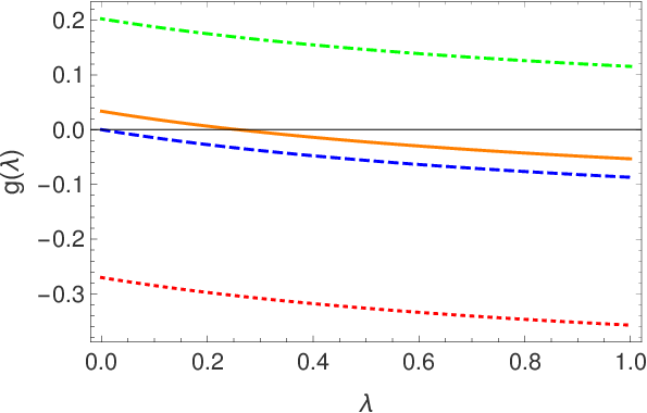
From Eq. (56) and Eq. (57), we conclude that the contribution of the b4​Fb_{4F}-terms, generated by the four-fermion interactions, modifies the behavior of the renormalized mass, because they may change the sign of the function g⁡(λ)g(\lambda), as shown in Fig. 3. In Fig. 4, we plot the function m⁡(Λ)m(\Lambda). In general, there are three possible cases, namely: (A) g⁡(λ)<0g(\lambda)<0 for any λ\lambda, (B) g⁡(λ)>0g(\lambda)>0 for any λ\lambda, and (C) where either g⁡(λ)>0g(\lambda)>0 for λ>λc\lambda>\lambda_{c} or g⁡(λ)<0g(\lambda)<0 for λ<λc\lambda<\lambda_{c}. The critical point λc\lambda_{c} is obtained from g⁡(λc)=0g(\lambda_{c})=0. Obviously, only the case (C) allow us to control the renormalized mass by tunning the value of λ\lambda.

Next, let us consider the case (A). This is the regime where the renormalized mass is fully controlled by the electromagnetic interactions. Therefore, the sum over the b4​Fb_{4F}-term vanishes. In Fig. 5, we show a plot for such possibility. From table I, we conclude that there are six different combinations that fulfil this criteria. These are: (A.1) (ψ¯​ψ)2+(ψ¯​γ3​γ5​ψ)2\left(\bar{\psi}\psi\right)^{2}+\left(\bar{\psi}\gamma^{3}\gamma^{5}\psi\right)^{2}, (A.2) (ψ¯​ψ)2+(ψ¯​γ3​ψ)2+(ψ¯​γ5​ψ)2\left(\bar{\psi}\psi\right)^{2}+\left(\bar{\psi}\gamma^{3}\psi\right)^{2}+\left(\bar{\psi}\gamma^{5}\psi\right)^{2}, (A.3) (ψ¯​γμ​ψ)2+(ψ¯​γμ​γ3​ψ)2+(ψ¯​γμ​γ5​ψ)2\left(\bar{\psi}\gamma^{\mu}\psi\right)^{2}+\left(\bar{\psi}\gamma^{\mu}\gamma^{3}\psi\right)^{2}+\left(\bar{\psi}\gamma^{\mu}\gamma^{5}\psi\right)^{2} (where (ψ¯​γμ​ψ)2\left(\bar{\psi}\gamma^{\mu}\psi\right)^{2} can be replaced by (ψ¯​γμ​γ3​γ5​ψ)2\left(\bar{\psi}\gamma^{\mu}\gamma^{3}\gamma^{5}\psi\right)^{2}), and (A.4) (ψ¯​γμ​γ3​ψ)2+(ψ¯​γ3​γ5​ψ)2+(ψ¯​γ3​ψ)2+(ψ¯​γ5​ψ)2\left(\bar{\psi}\gamma^{\mu}\gamma^{3}\psi\right)^{2}+\left(\bar{\psi}\gamma^{3}\gamma^{5}\psi\right)^{2}+\left(\bar{\psi}\gamma^{3}\psi\right)^{2}+\left(\bar{\psi}\gamma^{5}\psi\right)^{2} (where (ψ¯​γμ​γ3​ψ)2\left(\bar{\psi}\gamma^{\mu}\gamma^{3}\psi\right)^{2} can be replaced by (ψ¯​γμ​γ5​ψ)2\left(\bar{\psi}\gamma^{\mu}\gamma^{5}\psi\right)^{2}). In the case (A), we conclude that m⁡(Λ)→0m(\Lambda)\rightarrow 0 as Λ→∞\Lambda\rightarrow\infty.

In the case (B), we need combinations that always provide g⁡(λ)g(\lambda) positive. In this regime, the influence of the four-fermion interactions is dominant over the contribution of the electromagnetic interactions. Therefore, the sum over the b4​Fb_{4F}-term must be larger than the first term in the rhs of Eq. (57), for any λ\lambda. In Fig. 5, we show a plot for such possibility. From table I, we conclude that there are seven different combinations that fulfil this criteria. These are: (B.1) (ψ¯​γμ​γ3​ψ)2+(ψ¯​γμ​γ5​ψ)2\left(\bar{\psi}\gamma^{\mu}\gamma^{3}\psi\right)^{2}+\left(\bar{\psi}\gamma^{\mu}\gamma^{5}\psi\right)^{2}, (B.2) (ψ¯​ψ)2+(ψ¯​γμ​γ3​ψ)2\left(\bar{\psi}\psi\right)^{2}+\left(\bar{\psi}\gamma^{\mu}\gamma^{3}\psi\right)^{2} (where (ψ¯​γμ​γ3​ψ)2\left(\bar{\psi}\gamma^{\mu}\gamma^{3}\psi\right)^{2} can be replaced by (ψ¯​γμ​γ5​ψ)2\left(\bar{\psi}\gamma^{\mu}\gamma^{5}\psi\right)^{2}), (B.3) (ψ¯​γμ​γ3​ψ)2+(ψ¯​γ3​ψ)2\left(\bar{\psi}\gamma^{\mu}\gamma^{3}\psi\right)^{2}+\left(\bar{\psi}\gamma^{3}\psi\right)^{2}, and (B.4) (ψ¯​γμ​γ5​ψ)2+(ψ¯​γ3​ψ)2\left(\bar{\psi}\gamma^{\mu}\gamma^{5}\psi\right)^{2}+\left(\bar{\psi}\gamma^{3}\psi\right)^{2} (in the last two combinations (ψ¯​γ3​ψ)2\left(\bar{\psi}\gamma^{3}\psi\right)^{2} can replaced by (ψ¯​γ5​ψ)2\left(\bar{\psi}\gamma^{5}\psi\right)^{2}). In the case (B), we conclude that m⁡(Λ)→∞m(\Lambda)\rightarrow\infty as Λ→∞\Lambda\rightarrow\infty.

In the case (C), the sign of g⁡(λ)g(\lambda) changes after crossing the point λc\lambda_{c}. In this regime, the renormalized mass is described by the competition of electromagnetic and four-fermion interactions, where both of them are relevant. We find two possible values for the critical coupling constant, namely, λcmax=0.66\lambda^{{\rm max}}_{c}=0.66 and λcmin=0.26\lambda^{{\rm min}}_{c}=0.26. From table I, we find seven combinations that provide λcmax\lambda^{{\rm max}}_{c}, given by: (C.1.A) (ψ¯​ψ)2(\bar{\psi}\psi)^{2}, (C.2.A) (ψ¯​γμ​γ3​ψ)2+(ψ¯​γ3​γ5​ψ)2\left(\bar{\psi}\gamma^{\mu}\gamma^{3}\psi\right)^{2}+\left(\bar{\psi}\gamma^{3}\gamma^{5}\psi\right)^{2}, (C.3.A) (ψ¯​ψ)2+(ψ¯​γμ​γ3​ψ)2+(ψ¯​γ3​γ5​ψ)2+(ψ¯​γ3​ψ)2+(ψ¯​γ5​ψ)2\left(\bar{\psi}\psi\right)^{2}+\left(\bar{\psi}\gamma^{\mu}\gamma^{3}\psi\right)^{2}+\left(\bar{\psi}\gamma^{3}\gamma^{5}\psi\right)^{2}+\left(\bar{\psi}\gamma^{3}\psi\right)^{2}+\left(\bar{\psi}\gamma^{5}\psi\right)^{2}, and (C.4.A) (ψ¯​γμ​γ3​ψ)2+(ψ¯​γ3​ψ)2+(ψ¯​γ5​ψ)2\left(\bar{\psi}\gamma^{\mu}\gamma^{3}\psi\right)^{2}+\left(\bar{\psi}\gamma^{3}\psi\right)^{2}+\left(\bar{\psi}\gamma^{5}\psi\right)^{2} (in each of the previous combinations we can change (ψ¯​γμ​γ3​ψ)2\left(\bar{\psi}\gamma^{\mu}\gamma^{3}\psi\right)^{2} by (ψ¯​γμ​γ5​ψ)2\left(\bar{\psi}\gamma^{\mu}\gamma^{5}\psi\right)^{2}). On the other hand, for finding λcmin\lambda^{{\rm min}}_{c}, there are six possibilities, namely, (C.1.B) (ψ¯​ψ)2+(ψ¯​γ3​ψ)2(\bar{\psi}\psi)^{2}+(\bar{\psi}\gamma^{3}\psi)^{2} and (C.2.B) (ψ¯​ψ)2+(ψ¯​γ5​ψ)2(\bar{\psi}\psi)^{2}+(\bar{\psi}\gamma^{5}\psi)^{2}, (C.3.B) (ψ¯​γμ​γ3​ψ)2+(ψ¯​γ3​γ5​ψ)2+(ψ¯​γ3​ψ)2\left(\bar{\psi}\gamma^{\mu}\gamma^{3}\psi\right)^{2}+\left(\bar{\psi}\gamma^{3}\gamma^{5}\psi\right)^{2}+\left(\bar{\psi}\gamma^{3}\psi\right)^{2}, (C.4.B) (ψ¯​γμ​γ3​ψ)2+(ψ¯​γ3​γ5​ψ)2+(ψ¯​γ5​ψ)2\left(\bar{\psi}\gamma^{\mu}\gamma^{3}\psi\right)^{2}+\left(\bar{\psi}\gamma^{3}\gamma^{5}\psi\right)^{2}+\left(\bar{\psi}\gamma^{5}\psi\right)^{2}, (C.5.B) (ψ¯​γμ​γ5​ψ)2+(ψ¯​γ3​γ5​ψ)2+(ψ¯​γ3​ψ)2\left(\bar{\psi}\gamma^{\mu}\gamma^{5}\psi\right)^{2}+\left(\bar{\psi}\gamma^{3}\gamma^{5}\psi\right)^{2}+\left(\bar{\psi}\gamma^{3}\psi\right)^{2}, and (C.6.B) (ψ¯​γμ​γ5​ψ)2+(ψ¯​γ3​γ5​ψ)2+(ψ¯​γ5​ψ)2\left(\bar{\psi}\gamma^{\mu}\gamma^{5}\psi\right)^{2}+\left(\bar{\psi}\gamma^{3}\gamma^{5}\psi\right)^{2}+\left(\bar{\psi}\gamma^{5}\psi\right)^{2}. The case (C) clearly provides two possible asymptotic behaviors for m⁡(Λ)m(\Lambda), see Fig. 5.

Refer to caption
Figure 3: The function g⁡(λ)g(\lambda) in the interval λ∈[0.1,1]\lambda\in\left[0.1,1\right] with N=4N=4. We plot Eq. (57) for four different combinations of the four-fermion interactions. The continuos line is obtained from the (ψ¯​ψ)2(\bar{\psi}\psi)^{2} and (ψ¯​γ3​ψ)2(\bar{\psi}\gamma^{3}\psi)^{2} interactions, which provides ∑{b4​F}b4​F=1/3​π2\sum_{\{b_{4F}\}}b_{4F}=1/3\pi^{2}. In this case, we find λcmin=0.26\lambda^{\rm min}_{c}=0.26. The dashed line is the combination of (ψ¯​ψ)2(\bar{\psi}\psi)^{2} and (ψ¯​γ3​γ5​ψ)2(\bar{\psi}\gamma^{3}\gamma^{5}\psi)^{2} interactions, where ∑{b4​F}b4​f=0\sum_{\{b_{4F}\}}b_{4f}=0. The dotted line is obtained from the (ψ¯​γμ​ψ)2(\bar{\psi}\gamma^{\mu}\psi)^{2} interaction, where b4​F=−8/3π2b_{4F}=-8/3\pi^{2}. The dashed-dotted line is obtained from the (ψ¯​ψ)2(\bar{\psi}\psi)^{2} and (ψ¯​γμ​γ3​ψ)2(\bar{\psi}\gamma^{\mu}\gamma^{3}\psi)^{2} interactions, where ∑{b4​F}b4​F=2/π2\sum_{\{b_{4F}\}}b_{4F}=2/\pi^{2}. Note that only for the continuos line we have a critical point.
Refer to caption
Figure 4: The behavior of m⁡(Λ)m(\Lambda). We plot Eq. (56) considering the (ψ¯​ψ)2(\bar{\psi}\psi)^{2} and (ψ¯​γ3​ψ)2(\bar{\psi}\gamma^{3}\psi)^{2} interactions, which provides λcmin=0.26\lambda^{\rm min}_{c}=0.26. For the line, we use λ=0.1\lambda=0.1 while for the dashed line we use λ=0.5\lambda=0.5. We consider N=4N=4 for both curves.

In Ref. fernandez, it has been shown that the combination of electromagnetic and Gross-Neveu interactions yields λcmax=0.66\lambda^{\rm max}_{c}=0.66, which is our case (C.1.A). We believe that combinations with a minimal critical coupling constant λcmin=0.26\lambda^{\rm min}_{c}=0.26, see Fig. 4, are likely to provide an easier controlling of the renormalized mass. Indeed, because screening effects, due to the substrates, decrease the value of λ\lambda, hence, the phase when λ>λc\lambda>\lambda_{c} becomes harder to achieve experimentally. From the experimental point of view, it is possible to relate the energy scale Λ\Lambda with the electronic density nn (the number of electrons by unit of surface area) by using the scaling law Λ→n1/2\Lambda\rightarrow n^{1/2} sarman. The value of nn is controlled by a gate voltage fernandez. We believe that our results may be relevant for describing a more realistic process of mass renormalization. Obviously, the four-fermion interactions should be related with microscopic interactions, such as mechanical vibrations, impurities, and disorder in the honeycomb lattice.

Refer to caption
Figure 5: The behavior of m⁡(Λ)m(\Lambda). We plot Eq. (56) with N=4N=4 and λ=0.4\lambda=0.4. The continuos line is obtained from the (ψ¯​ψ)2(\bar{\psi}\psi)^{2} and (ψ¯​γ3​γ5​ψ)2(\bar{\psi}\gamma^{3}\gamma^{5}\psi)^{2} interactions (the same curve holds when we replace γ3\gamma_{3} by γ5\gamma_{5}). The dashed line is obtained from the Thirring interaction (ψ¯​γμ​ψ)2(\bar{\psi}\gamma^{\mu}\psi)^{2}. The dotted line is obtained from (ψ¯​ψ)2(\bar{\psi}\psi)^{2} and (ψ¯​γμ​γ3​ψ)2(\bar{\psi}\gamma^{\mu}\gamma^{3}\psi)^{2} interactions.

VI SUMMARY AND OUTLOOK

The experimental realization of two-dimensional materials, where the quasiparticles obey a Dirac-like equation, allow us to consider a quantum-electrodynamical approach in order to describe electronic interactions in these systems. In particular, the experimental observation geim of the Fermi velocity renormalization vozmediano in graphene confirms that electronic interactions are indeed relevant. Recently, the description of the band gap renormalization fernandez in WSe2 WSe and MoS2 MoS increases this window of possible applications, using standard renormalization group equations, as in Ref. foster. Within a nonperturbative regime, one can also consider the description of excitonic spectrum Exc, dynamical mass generation popovici, and the realization of parity anomaly PRX through a quantum valley Hall effect. Beyond these regimes, one can consider the microscopic interactions by taking models that simultaneously describe both electromagnetic and four-fermion interactions. These cases, however, have been less discussed in literature EbertFF.

In this work we gave a step forward in this picture by considering an effective low-energy model that is suitable for calculating the effects of both electromagnetic and the generalized four-fermion interactions with O⁡(4)O(4) symmetry. As a concrete application, we calculated the renormalized mass m⁡(Λ)m(\Lambda), within the large-NN approximation. This may be measured by looking at the energy gap between the valence (negative energy) and conduction (positive energy) bands at the valleys of the honeycomb lattice WSe; MoS. For the sake of comparison with the experimental data, we may replace the energy scale Λ\Lambda by the electron density nn, through the transform Λ→n1/2\Lambda\rightarrow n^{1/2}, which is true for two-dimensional electrons vozmediano; fernandez. Our result shows that an ultraviolet fixed point λc\lambda_{c} is generated, implying that m⁡(Λ)m(\Lambda) does not renormalizes at λ=λc\lambda=\lambda_{c}. Thereafter, we find that there exist two possible values for λc\lambda_{c}, namely, the maximal value λcmax=0.66\lambda^{\rm max}_{c}=0.66 and the minimal value λcmin=0.26\lambda^{\rm min}_{c}=0.26 (this does not depends on the constant NN). The kind of value we find depends on the combinations of four-fermion interactions we are considering in the initial model. This provides a possible tuning mechanism for the renormalized mass, because the behavior of m⁡(Λ)m(\Lambda) changes when λ=π​α/4\lambda=\pi\alpha/4 is either larger or less than λc\lambda_{c}.

The model presented here is also suitable for investigating the ultrarelativistic limit of the Dirac-like materials, where vF​(n)→cv_{F}(n)\rightarrow c as n→0n\rightarrow 0, where cc is the light velocity. Because our current results only describe the regime where vF​(n)≪cv_{F}(n)\ll c (the static limit), it would be interesting to understand the behavior of the renormalized mass in the dynamical limit. We shall consider this generalization elsewhere.

Acknowledgement

L. F. is partially supported by Coordenação de Aperfeiçoamento de Pessoal de Nível Superior Brasil (CAPES), finance code 001. V. S. A. and L. O. N. are partially supported by Conselho Nacional de Desenvolvimento Científico e Tecnológico (CNPq) and by CAPES/NUFFIC, finance code 0112. F. P. acknowledge the financial support from Dirección De Investigación De La Universidad De La Frontera Grant No. DI20-0005.

Appendix A Vacuum polarization tensor of four-fermion interactions

Equation (18) represents the general form of the one-loop quantum correction to the auxiliary-field propagators. Here, we provide a few details of the computation of this term for the case of the Thirring interaction where the vertex is φμ​ψ¯​γμ​ψ\varphi_{\mu}\bar{\psi}\gamma^{\mu}\psi. In this case, we have

Πφμμ​ν(p¯)=−1N​vF2Tr∫d3​k(2​π)3γμSF(p¯+k)γνSF(k).\Pi^{\mu\nu}_{\varphi_{\mu}}(\bar{p})\!=\!\!-\frac{1}{Nv_{F}^{2}}{\rm Tr}\!\!\int\!\!\frac{d^{3}k}{(2\pi)^{3}}\gamma^{\mu}S_{F}\!\left(\bar{p}+k\right)\gamma^{\nu}S_{F}\left(k\right). (A.1)

Next, we use Eq. (6) and the following trace operations over the Dirac matrices, namely,

Tr⁡[γμ​γν]\displaystyle{\rm Tr}[\gamma^{\mu}\gamma^{\nu}] =−4​δμ​ν,\displaystyle=-4\delta^{\mu\nu}, (A.2)
Tr⁡[γμ​γα​γν​γβ]\displaystyle{\rm Tr}\left[\gamma^{\mu}\gamma^{\alpha}\gamma^{\nu}\gamma^{\beta}\right] =(δμ​α​δν​β−δμ​ν​δα​β+δμ​β​δν​α),\displaystyle=4\!\left(\delta^{\mu\alpha}\!\delta^{\nu\beta}\!\!-\delta^{\mu\nu}\delta^{\alpha\beta}+\delta^{\mu\beta}\delta^{\nu\alpha}\right), (A.3)

which are useful properties to expand the numerator of Eq. (A.1). After calculating the trace over the Dirac matrices, this numerator reads

(p¯+k)μ​kν+(p¯+k)ν​kμ−δμ​ν​[(p¯+k)⋅k+m2].(\bar{p}+k)^{\mu}k^{\nu}+(\bar{p}+k)^{\nu}k^{\mu}-\delta^{\mu\nu}\left[(\bar{p}+k)\cdot k+m^{2}\right]. (A.4)

On the other hand, we use the Feynman parametrization in the denominator, which becomes equal to

[(k+x​p¯)2+x⁡(1+x)​p¯2+m2]2.\left[(k+x\bar{p})^{2}+x(1+x)\bar{p}^{2}+m^{2}\right]^{2}. (A.5)

Thereafter, in order to eliminate symmetric-loop integrals, we made a variable change k→k−x​p¯k\rightarrow k-x\bar{p} and, by using Lorentz invariance, we finally find a simplified equation for Πφμμ​ν​(p¯)\Pi^{\mu\nu}_{\varphi_{\mu}}(\bar{p}), namely,

Πφμμ​ν​(p¯)=−4vF2∫10dx{∫d3​k(2​π)3(23−1)​δμ​ν​k2[k2+Δ1]2∫d3​k(2​π)3(δμ​ν−2​p¯μ​p¯νp¯2)​x​(−x)​p¯2−δμ​ν​m2[k2+Δ1]2}\begin{split}\Pi^{\mu\nu}_{\varphi_{\mu}}(\bar{p})&=-\frac{4}{v_{F}^{2}}\int^{1}_{0}dx\left\{\int\frac{d^{3}k}{(2\pi)^{3}}\frac{\left(\frac{2}{3}-1\right)\delta^{\mu\nu}k^{2}}{\left[k^{2}+\Delta_{1}\right]^{2}}\right.\\ &\left.\!\!\!\int\!\!\frac{d^{3}k}{(2\pi)^{3}}\frac{\left(\!\delta^{\mu\nu}\!\!-\!\!2\frac{\bar{p}^{\mu}\bar{p}^{\nu}}{\bar{p}^{2}}\right)\!x(1\!-\!x)\bar{p}^{2}\!\!-\!\delta^{\mu\nu}m^{2}}{\left[k^{2}+\Delta_{1}\right]^{2}}\right\}\end{split} (A.6)

with Δ1=x⁡(1−x)​p¯2+m2\Delta_{1}=x(1-x)\bar{p}^{2}+m^{2}. After solving the integrals, using the dimensional regularization scheme, we find

Πφμμ​ν​(p¯)=−p¯2π​vF2{m22​p¯2+p¯2−4​m24​p¯2​p¯2×arcsin[p¯2p¯2+4​m2]}ℙ¯μ​ν.\begin{split}\Pi^{\mu\nu}_{\varphi_{\mu}}(\bar{p})&=-\frac{\bar{p}^{2}}{\pi v_{F}^{2}}\left\{\frac{\sqrt{m^{2}}}{2\bar{p}^{2}}+\frac{\bar{p}^{2}-4m^{2}}{4\bar{p}^{2}\sqrt{\bar{p}^{2}}}\right.\\ &\left.\times\arcsin\left[\sqrt{\frac{\bar{p}^{2}}{\bar{p}^{2}+4m^{2}}}\right]\right\}\mathbb{\bar{P}}^{\mu\nu}.\end{split} (A.7)

In the cases of other auxiliary fields, we use that γ3\gamma^{3} and γ5\gamma^{5} anti-commute with γμ\gamma^{\mu} and between them, furthermore, (γ3)2=(γ5)2=𝟙(\gamma^{3})^{2}=(\gamma^{5})^{2}=\mathbbm{1}. Hence, it follows some useful properties, given by

Tr⁡[γ3​(5)​γ3​(5)]=4,\displaystyle{\rm Tr}[\gamma^{3(5)}\gamma^{3(5)}]=4, (A.8)
Tr⁡[γ3​(5)​γα​γ3​(5)​γβ]=4​δα​β,\displaystyle{\rm Tr}\left[\gamma^{3(5)}\gamma^{\alpha}\gamma^{3(5)}\gamma^{\beta}\right]=4\delta^{\alpha\beta}, (A.9)
Tr⁡[γ3​γ5​γ3​γ5]=−4,\displaystyle{\rm Tr}\left[\gamma^{3}\gamma^{5}\gamma^{3}\gamma^{5}\right]=-4, (A.10)
Tr⁡[γμ​γ3​(5)​γα​γν​γ3​(5)​γβ]=Tr⁡[γμ​γα​γν​γβ],\displaystyle{\rm Tr}\left[\gamma^{\mu}\gamma^{3(5)}\gamma^{\alpha}\gamma^{\nu}\gamma^{3(5)}\gamma^{\beta}\right]={\rm Tr}\left[\gamma^{\mu}\gamma^{\alpha}\gamma^{\nu}\gamma^{\beta}\right], (A.11)
Tr⁡[γ3​γ5​γα​γ3​γ5​γβ]=4​δα​β\displaystyle{\rm Tr}\left[\gamma^{3}\gamma^{5}\gamma^{\alpha}\gamma^{3}\gamma^{5}\gamma^{\beta}\right]=4\delta^{\alpha\beta} (A.12)
Tr⁡[γμ​γ3​γ5​γα​γν​γ3​γ5​γβ]=−Tr⁡[γμ​γα​γν​γβ].\displaystyle{\rm Tr}\left[\gamma^{\mu}\gamma^{3}\gamma^{5}\gamma^{\alpha}\gamma^{\nu}\gamma^{3}\gamma^{5}\gamma^{\beta}\right]=-{\rm Tr}\left[\gamma^{\mu}\gamma^{\alpha}\gamma^{\nu}\gamma^{\beta}\right]. (A.13)

We obtain Πφ3​(p¯)\Pi_{\varphi_{3}}(\bar{p}) and Πφ5​(p¯)\Pi_{\varphi_{5}}(\bar{p}) using Γl=γ3\Gamma^{l}=\gamma^{3} or γ5\gamma^{5} respectively, in Eq. (18). Then, we implement the same procedure for solve Eq. (A.1) together with Eqs. (A.8) and (A.9), of form that

Πφ3​(p¯)=p¯2π​vF2​[m2p¯2+12​arcsin⁡(p¯2p¯2+4​m2)],\Pi_{\varphi_{3}}\!(\bar{p})\!=\!\!\frac{\sqrt{\bar{p}^{2}}}{\pi v_{F}^{2}}\!\left[\!\sqrt{\frac{m^{2}}{\bar{p}^{2}}}\!+\!\frac{1}{2}\!\arcsin\left(\!\!\sqrt{\frac{\bar{p}^{2}}{\bar{p}^{2}+4m^{2}}}\right)\!\right], (A.14)

for Πφ5​(p¯)\Pi_{\varphi_{5}}(\bar{p}) we have the same previous result. We use Γl=γμ​γ3\Gamma^{l}=\gamma^{\mu}\gamma^{3} (or γμ​γ5\gamma^{\mu}\gamma^{5}) in Eq. (18) and Eqs. (A.9) and (A.11) for we obtain Πφμ​3​(p¯)\Pi_{\varphi_{\mu 3}}(\bar{p}) (or Πφμ​5​(p¯)\Pi_{\varphi_{\mu 5}}(\bar{p})), being

Πφμ​3μ​ν(p¯)=−p¯22​π​vF2{[m2p¯2+p¯2+4​m22​p¯2×arcsin(p¯2p¯2+4​m2)]ℙ¯μ​ν+2m2p¯2δμ​ν},\begin{split}\Pi_{\varphi_{\mu 3}}^{\mu\nu}&(\bar{p})=-\frac{\sqrt{\bar{p}^{2}}}{2\pi v_{F}^{2}}\left\{\left[\sqrt{\frac{m^{2}}{\bar{p}^{2}}}+\frac{\bar{p}^{2}+4m^{2}}{2\bar{p}^{2}}\right.\right.\\ &\left.\left.\times\arcsin\left(\!\!\sqrt{\!\frac{\bar{p}^{2}}{\bar{p}^{2}+4m^{2}}}\,\right)\!\right]\mathbb{\bar{P}}^{\mu\nu}\!+2\frac{m^{2}}{\bar{p}^{2}}\delta^{\mu\nu}\right\},\end{split} (A.15)

using Γl=γ3​γ5\Gamma^{l}=\gamma^{3}\gamma^{5} in Eq. (18) together with Eqs. (A.10) and (A.12) we obtain

Π35​(p¯)=−p¯2π​vF2[m2p¯2+p¯2+4​m22​p¯2×arcsin(p¯2p¯2+4​m2)],\begin{split}\Pi_{35}(\bar{p})&=-\frac{\sqrt{\bar{p}^{2}}}{\pi v_{F}^{2}}\left[\sqrt{\frac{m^{2}}{\bar{p}^{2}}}+\frac{\bar{p}^{2}+4m^{2}}{2\bar{p}^{2}}\right.\\ &\left.\times\arcsin\left(\sqrt{\frac{\bar{p}^{2}}{\bar{p}^{2}+4m^{2}}}\right)\right]\end{split}, (A.16)

by last we may obtain Πφμ​35μ​ν​(p¯)\Pi_{\varphi_{\mu 35}}^{\mu\nu}(\bar{p}) by replacing Γl\Gamma^{l} by γμ​γ3​γ5\gamma^{\mu}\gamma^{3}\gamma^{5} in Eq. (18) and using the trace operation given by Eqs. (A.12) and (A.13), so

Πφμ​35μ​ν​(p¯)=p¯2π​vF2[m22​p¯2+p¯2−4​m24​p¯2​p¯2×arcsin(p¯2p¯2+4​m2)]ℙ¯μ​ν.\begin{split}\Pi^{\mu\nu}_{\varphi_{\mu 35}}(\bar{p})&=\frac{\bar{p}^{2}}{\pi v_{F}^{2}}\left[\frac{\sqrt{m^{2}}}{2\bar{p}^{2}}+\frac{\bar{p}^{2}-4m^{2}}{4\bar{p}^{2}\sqrt{\bar{p}^{2}}}\right.\\ &\left.\times\arcsin\left(\sqrt{\frac{\bar{p}^{2}}{\bar{p}^{2}+4m^{2}}}\right)\right]\mathbb{\bar{P}}^{\mu\nu}.\end{split} (A.17)

References

  • (1) W. Thirring, A soluble relativistic field theory, Ann. Phys. (N.Y.) 3, 91 (1958).
  • (2) Y. Nambu and Jona-Lasinio, Dynamical Model of Elementary Particles Based on an Analogy with Superconductivity. I, Phys. Rev. 122, 345 (1961); Y. Nambu and Jona-Lasinio, Dynamical Model of Elementary Particles Based on an Analogy with Superconductivity. II, Phys. Rev. 124, 246 (1961).
  • (3) R. T. Cahill and C. D. Roberts, Soliton bag models of hadrons from QCD, Phys. Rev. D 32, 2419 (1985); D. Dyakonov and V. Yu Petrov, A theory of light quarks in the instanton vacuum, Nucl. Phys. B 272, 457 (1986); H. Reinhardt, Hadronization of quark flavor dynamics, Phys. Lett. B 244, 316 (1990); H. Rejnhardt, Bosonization of QCD in the field strength approach, Phys. Lett. B 257, 375 (1991).
  • (4) T. Hatsuda and T. Kunihiro, QCD phenomenology based on a chiral effective Lagrangian, Phys. Rep. 247, 221 (1994).
  • (5) F. J. Dyson, The Radiation Theories of Tomonaga, Schwinger, and Feynman, Phys. Rev. 75, 486 (1949); F. J. Dyson, The SS Matrix in Quantum Electrodynamics, Phys. Rev. 75, 1736 (1949).
  • (6) C. de Calan, P. A. Faria da Veiga, J. Magnen, and R. Sénéor, Constructing the three-dimensional Gross-Neveu model with a large number of flavor components, Phys. Rev. Lett. 66, 3233 (1991); H. Gies and L. Janssen, UV fixed-point structure of the three-dimensional Thirring model, Phys. Rev. D 82, 085018 (2010).
  • (7) David J. Gross, in: Roger Balian, Jean Zinn-Justin (Eds.), Proceedings of Lês Houches, Session XXVIII, 1975, North-Holland Publishing Co, Amsterdam, 1976; B. Rosenstein, B.J. Warr, S.H. Park, Four-fermion theory is renormalizable in 2+1 dimensions, Phys. Rev. Lett. 62, 1433 (1989).
  • (8) M. Gomes, V. O. Rivelles, A. J. da Silva, Dynamical parity violation and the Chern-Simons term, Phys. Rev. D 41, 1363 (1990); M. Gomes, R. S. Mendes, R. F. Ribeiro, and A. J. da Silva, Gauge structure, anomalies, and mass generation in a three-dimensional Thirring model, Phys. Rev. D 43, 3516 (1991).
  • (9) J. Hubbard, Calculation of Partition Functions, Phys. Rev. Lett. 3, 77 (1959).
  • (10) K. S. Novoselov, A. K. Geim, S. V. Morozov, D. Jiang, Y. Zhang, S. V. Dubonos, I. V. Grigorieva, and A. A. Firsov, Electric field effect in atomically thin carbon films, Science 306, 666 (2004).
  • (11) B. Lalmi, H. Oughaddou, H. Enriquez, A. Kara, S. Vizzini, B. Ealet, and B. Aufray, Epitaxial growth of a silicene sheet, Appl. Phys. Lett. 97, 223109 (2010).
  • (12) G. Wang, A. Chernikov, M. M. Glazov, T. F. Heinz, X. Marie, T. Amand, and B. Urbaszek, Colloquium: Excitons in atomically thin transition metal dichalcogenides, Rev. Mod. Phys. 90, 021001 (2018).
  • (13) P.-L. Zhao, A.-M. Wang, and G.-Z. Liu, Condition for the emergence of a bulk Fermi arc in disordered Dirac-fermion systems, Phys. Rev. B 98, 085150 (2018).
  • (14) J. Wang, Role of four-fermion interaction and impurity in the states of two-dimensional semi-Dirac materials, J. Phys. Condensed Matter 30, 12 (2018).
  • (15) E. C. Marino, Quantum electrodynamics of particles on a plane and the Chern-Simons theory, Nucl. Phys. B408, 551. (1993).
  • (16) L. Fernández, V. S. Alves, L. O. Nascimento, F. Penña, M. Gomes, and E. C. Marino, Renormalization of the band gap in 2D materials through the competition between electromagnetic and four-fermion interactions in large N expansion, Phys. Rev. D 102, 016020 (2020).
  • (17) P. V. Nguyen, N. C. Teutsch, N. P. Wilson, J. Kahn, X. Xia, A. J. Graham, V. Kandyba, A. Giampietri, A. Barinov, G. C. Constantinescu, N. Yeung, N. D. M. Hine, X. Xu, D. H. Cobden, and N. R. Wilson, Visualizing electrostatic gating effects in two-dimensional heterostructures, Nature (London) 572, 220 (2019).
  • (18) F. Liu, M. E. Ziffer, K. R. Hansen, J. Wang, and X. Zhu, Direct Determination of Band-Gap Renormalization in the Photoexcited Monolayer M​o​S2MoS_{2}, Phys. Rev. Lett. 122, 246803 (2019).
  • (19) M. A. H. Vozmediano and F. Guinea, Effect of Coulomb interactions on the physical observables of graphene, Phys. Scr. T146, 014015 (2012); F. de Juan, A. G. Grushin, and M. A. H. Vozmediano, Renormalization of Coulomb inter- action in graphene: Determining observable quantities, Phys. Rev. B 82, 125409 (2010); J. González, F. Guinea, and M. A. H. Vozmediano, Marginal-Fermi-liquid behavior from two-dimensional Coulomb interaction, Phys. Rev. B 59, R2474 (1999).
  • (20) B. Charneski, M. Gomes, T. Mariz, J. R. Nascimento, and A. J. da Silva, Dynamical Lorentz symmetry breaking in 3D and charge fractionalization, Phys. Rev. D 79, 065007 (2009).
  • (21) N. Menezes, V. S. Alves, E. C. Marino, L. Nascimento, L. O. Nascimento, and C. Morais Smith, Spin g-factor due to electronic interactions in graphene, Phys. Rev. B 95, 245138 (2017).
  • (22) E. C. Marino, Quantum Field Theory Approach to Condensed Matter Physics, Cambridge University Press, (2017).
  • (23) J.-R. Wang, G.-Z. Liu, and C.-J. Zhang, Renormalization of fermion velocity in finite temperature QED3, Phys. Rev. D 93, 045017 (2016).
  • (24) T. Son, Quantum critical point in graphene approached in the limit of infinitely strong Coulomb interaction, Phys. Rev. B 75, 235423 (2007).
  • (25) S. Das Sarma, S. Adam, E. H. Hwang, and E. Rossi, Electronic transport in two-dimensional graphene, Rev. Mod. Phys. 83, 407 (2011); S. Das Sarma, E. H. Hwang, and H. Min, Carrier screening, transport, and relaxation in three-dimensional Dirac semimetals, Phys. Rev. B 91, 035201 (2015).
  • (26) D. C. Elias, R. V. Gorbachev, A. S. Mayorov, S. V. Morozov, A. A. Zhukov, P. Blake, L. A. Ponomarenko, I. V. Grigorieva, K. S. Novoselov, F. Guinea, and A.K. Geim, Dirac cones reshaped by interaction effects in suspended graphene, Nat. Phys. 7, 701 (2011).
  • (27) M. S. Foster and I. L. Aleiner, Grapehen via large N: A renormalization group study, Phys. Rev. B 77, 195413 (2008).
  • (28) E. C. Marino, L. O. Nascimento, V. S. Alves, N. Menezes, and C. M. Smith, Quantum-electrodynamical approach to the exciton spectrum in transition-metal dichalcogenides, 2D Materials 5, 041006 (2018).
  • (29) E. C. Marino, L. O. Nascimento, V. S. Alves, and C. M. Smith, Interaction Induced Quantum Valley Hall Effect in Graphene, Phys. Rev. X 5, 011040 (2015).
  • (30) C. Popovici, C. S. Fischer, and L. von Smekal, Fermi velocity renormalization and dynamical gap generation in graphene, Phys. Rev. B 88, 205429 (2013).
  • (31) D. Ebert, K. G. Klimenko, P. B. Kolmakov, V. Ch. Zhukovsky, Phase transitions in hexagonal, graphene-like lattice sheets and nanotubes under the influence of external conditions, Annals of Physics 371, 254 (2016).