The equilibrium points and stability of grid-connected synchronverters

Most distributed generators are connected to the utility grid via inverters that rely on various control algorithms to maintain synchronism. They usually offer no inertia, and behave as controlled current sources that produce fluctuating power. Numerous researchers are investigating how the future power grids should be controlled when inverters become dominant, offering competing control algorithms for grid-forming converters, see for instance the recent study [28]. One of the proposed approaches is to emulate the behavior of synchronous generators (SG), so that an inverter-based grid behaves like one based on SG, see for instance [4, 7, 9, 16, 19, 23, 28, 31, 36]. This has many advantages, such as backward compatibility with the current grid, well known black start and fault ride-through procedures, and well tested primary and secondary frequency and voltage support algorithms. Following [4], inverters that behave towards the utility grid like synchronous machines are called virtual synchronous machines (VSM).

One particular type of VSM are the synchronverters, introduced in [36, 37]. This type of inverter has attracted considerable attention, see for instance [1, 2, 5, 8, 26, 23, 33, 34, 35], and the recent survey [29]. The hardware of a synchronverter is similar to that of a conventional three phase inverter (with any number of DC levels, most commonly 3), the novelty is in the control algorithm. The only hardware difference is that some fast acting energy storage (typically, capacitors) is required on the DC bus, to provide the energy pulses (both positive and negative) needed for the emulation of rotor inertia. We base our modelling on the simplified circuit diagram of a grid-connected inverter in Fig. 1. Even though the synchronverter control scheme has evolved over time, all the formulations present in the literature share the same “basic control algorithm”. We base our modelling on this basic algorithm (see Fig. 2 in Sect. II for more details).

The stability of a SG (or VSM) connected to an infinite bus is a well motivated classical problem in the study of power systems. For instance, in [10, Sect. 12.3] and [13] we can find the stability analysis of a linearized second order approximation of this system. The same problem, with a more complex SG model, has been addressed in [24]. In the last decade, motivated by the growing interest in VSM-based grids, similar stability studies have been performed for more complex models of grid-connected VSM. In [3], [20] a fourth order model is formulated for a grid-connected VSM, and conditions on the parameters ensuring almost global asymptotic stability (aGAS) are derived, and in [17] a novel technique for state-space modeling of grid-connected converters is presented, with local stability evaluation via eigenvalues. In [27] a VSM model is developed, which contains a DC side that interacts with the AC side in an ingenious way, leading to aGAS of the VSM connected to an infinite bus. In the context of microgrids, stability results are derived in [6, 25, 32], and the importance of accurate modeling has been discussed, among others, in [30] and in the recent review [22]. The paper [18] presents an interesting equilibrium point analysis for microgrids interfaced via solid-state transformers. This analysis is then employed to develop a power sharing algorithm between the inverters.

This paper investigates the local asymptotic stability of a VSM functioning according to the basic synchronverter algorithm, when connected to a powerful grid modelled as an infinite bus. For this purpose, we formulate a fifth order grid-connected synchronverter model. This model is an extension of the fourth order model developed and analyzed in [3, 20], where the rotor (or field) current was assumed to be constant (thus ignoring the reactive power control loop). Using advanced mathematical methods, different sufficient conditions for almost global asymptotic stability of the fourth order model were derived in [3, 20]. Here we include the field current as the fifth state variable and we investigate the stability of the equilibrium points of the resulting fifth order system.

We derive a novel geometric representation of the fourth and fifth order models’ equilibrium points. We use extensively the mapping of equilibrium points into the power plane, where the coordinates are $P$ (the active power) and $Q$ (the reactive power). (In the language of differential geometry, the manifold of equilibrium points with positive field current is diffeomorphic to the power plane.) We show that, for a fixed prime mover torque and for field current values in a “reasonable” range, the image of the fourth order model equilibrium points in the power plane moves on a circle. The radius of this circle depends on the prime mover torque at the equilibrium. In the same geometric representation, we identify a stability sector for the fifth order model equilibrium points. This sector allows to determine a priori if certain reference values of active and reactive power will generate stable (or unstable) fifth order model equilibrium points.

The paper is organized as follows. In Sect. II we recover the fourth order grid-connected synchronverter model from [20, 21], and we extend it to a fifth order one, adding the field current to the state vector. In Sect. III the equilibrium points of the fourth order model are studied and the novel geometric representation is introduced. In Sect. IV we study the equilibrium points of the fifth order model and their representation in the power plane. In Sect. V we use results from Sect. III and IV to find a sufficient condition ensuring the stability of the fifth order model equilibrium points, employing singular perturbation methods developed in [15]. Based on this result, we characterize the power plane region corresponding to stable fifth order model equilibrium points. Finally, in Sect. VI we use two numerical examples to illustrate our novel geometric representation and our theoretical derivations.

In this section we construct the basic fifth order model of the synchronverter, following the terminology and notation of [20, 21, 37]. Note that the paper [21] has proposed five modifications to the synchronverter algorithm from [37], to improve its stability and performance. Of these, we adopt here only the two most important ones: a substantial increase of the effective size of the filter inductors, by using virtual inductors, and the improved anti-windup field current controller.

Our analysis is based on a simplified model of a synchronverter, given in Fig. 2. This model is simplified because it does not take into account the various low-pass filters that are included to reduce high frequency noise, and it also ignores most of the saturation blocks included in the algorithm (see [21, 5]) (however, the saturating integrator contained in the field current controller is considered). We also ignore start-up procedures and various protections. Including these features would result in a high-order model that is practically impossible to analyze rigorously. Moreover, ignoring the aforementioned features does not significantly alter the steady-state behaviour of the system, making our stability analysis relevant also for higher order models.

We proceed as follows: first we recover the fourth order model from [21] (where the field current $i_{f}$ was assumed to be a parameter). Then, we extend this model by including $i_{f}$ as a state variable, obtaining a fifth order model.

We denote by $\theta_{g}$ the grid angle and by ${\omega}_{g}$ the grid frequency, so that ${\omega}_{g}=\dot{\theta}_{g}$. The frequency ${\omega}_{g}$ is usually close to ${\omega}_{n}=100\pi$ rad/sec. We denote by $\theta$ the synchronverter virtual rotor angle, and by ${\omega}$ its angular velocity, so that ${\omega}=\dot{\theta}$. The difference $\delta=\theta-\theta_{g}$ is called the power angle. The notation $\widetilde{\cos}{\hbox{\hskip 1.0pt}}\theta$ and $\widetilde{\sin}{\hbox{\hskip 1.0pt}}\theta$ is defined by

$$\widetilde{\cos}{\hbox{\hskip 1.0pt}}\theta{\hbox{\hskip 1.0pt}}={\hbox{\hskip 1.0pt}}\left[\cos\theta\ {\hbox{\hskip 1.0pt}}\cos\left(\theta-\frac{2\pi}{3}\right)\ {\hbox{\hskip 1.0pt}}\cos\left(\theta+\frac{2\pi}{3}\right)\right]^{\top}{\hbox{\hskip 1.0pt}},$$

$$\widetilde{\sin}{\hbox{\hskip 1.0pt}}\theta{\hbox{\hskip 1.0pt}}={\hbox{\hskip 1.0pt}}\left[\sin\theta\ {\hbox{\hskip 1.0pt}}\sin\left(\theta-\frac{2\pi}{3}\right)\ {\hbox{\hskip 1.0pt}}\sin\left(\theta+\frac{2\pi}{3}\right)\right]^{\top}.$$

Then the grid voltage vector is

$$v{\hbox{\hskip 1.0pt}}={\hbox{\hskip 1.0pt}}\sqrt{\frac{2}{3}}V\widetilde{\sin}{\hbox{\hskip 1.0pt}}\theta_{g},$$

(1)

where $V$ is a positive constant or a slowly changing signal (this is the rms value of the line voltage).

Denote by $M_{f}>0$, the peak mutual inductance between the virtual rotor winding and any one stator winding, by $i_{f}$ the variable field current (or rotor current) and by $e$ the vector of electromotive forces, also called the internal synchronous voltage. We rewrite [37, eq. (4)]:

$$e{\hbox{\hskip 1.0pt}}={\hbox{\hskip 1.0pt}}M_{f}i_{f}{\omega}{\hbox{\hskip 1.0pt}}\widetilde{\sin}\theta-M_{f}\frac{{\rm d\hbox{\hskip 0.5pt}}i_{f}}{{\rm d\hbox{\hskip 0.5pt}}t}\widetilde{\cos}\theta$$

(2)

and we note that the variable current $i_{f}$ governs the amplitude of $e$. We apply the Park transformation

$$U(\theta)=\sqrt{\frac{2}{3}}\left[\begin{matrix}\vskip 2.84526pt\cos\theta&\cos(\theta-\frac{2\pi}{3})&\cos(\theta+\frac{2\pi}{3})\\ \vskip 2.84526pt-\sin\theta&-\sin(\theta-\frac{2\pi}{3})&-\sin(\theta+\frac{2\pi}{3})\\ 1/\sqrt{2}&1/\sqrt{2}&1/\sqrt{2}\end{matrix}\right]\vskip 2.84526pt$$

to (2). For any ${\mathbb{R}}^{3}$-valued signal $v$, the first two components of $U(\theta)v$ are called the $dq$ coordinates of $v$, denoted by $v_{d}$, $v_{q}$. By using the notation $m=\sqrt{3/2}{\hbox{\hskip 1.0pt}}M_{f}$, we represent the internal synchronous voltage $e$ in $dq$ coordinates as:

$$e_{d}{\hbox{\hskip 1.0pt}}={\hbox{\hskip 1.0pt}}-m\frac{{\rm d\hbox{\hskip 0.5pt}}i_{f}}{{\rm d\hbox{\hskip 0.5pt}}t},\hskip 20.00003pte_{q}{\hbox{\hskip 1.0pt}}={\hbox{\hskip 1.0pt}}-mi_{f}{\omega}.$$

(3)

The term $e_{d}$ can be neglected, because the rate of change of the field current is small, so that $e_{d}<<e_{q}$. Thus, in the synchronverter algorithm from [37] the approximation $e_{d}=0$ is adopted, and our analysis will follow this. (We remark that we did simulation experiments with $e_{d}$ as in (3), and the results were practically the same as for $e_{d}=0$.)

Applying the Park transformation to (1), we get the $dq$ representation of the grid voltage as

$$v_{d}{\hbox{\hskip 1.0pt}}={\hbox{\hskip 1.0pt}}-V\sin\delta,\hskip 20.00003ptv_{q}{\hbox{\hskip 1.0pt}}={\hbox{\hskip 1.0pt}}-V\cos\delta.$$

(4)

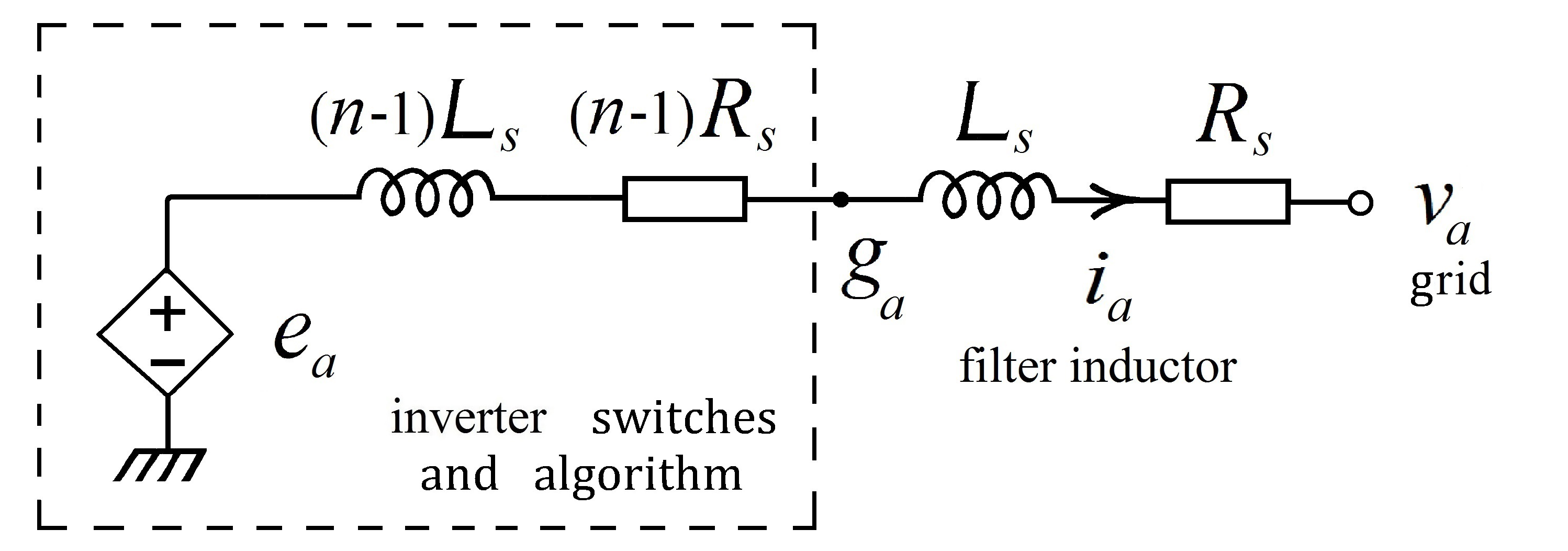
The control algorithm computes $g=[{\hbox{\hskip 1.0pt}}g_{a}\ {\hbox{\hskip 1.0pt}}g_{b}\ {\hbox{\hskip 1.0pt}}g_{c}]^{\top}$ and sends it to the switches in the power part (see Fig. 3). In the original synchronverter algorithm from [37], we have $g_{d}=e_{d}$ and $g_{q}=e_{q}$, i.e., the internal synchronous voltage $e$ from (2) is sent straight to the PWM signal generator. Here we consider the modified synchronverter equations according to [21], which contain the original algorithm as a special case, namely $n=1$. Writing [21, eq. (22)] in $dq$ coordinates, we have

$$g_{d}={\hbox{\hskip 1.0pt}}\frac{(n-1)v_{d}+e_{d}}{n},\ \ \ \ {\hbox{\hskip 1.0pt}}g_{q}={\hbox{\hskip 1.0pt}}\frac{(n-1)v_{q}+e_{q}}{n}{\hbox{\hskip 1.0pt}}.$$

The current sensors are placed after the filter capacitors, as shown in Fig. 1, to avoid the switching noise. From these measurements, the inductor currents $i_{a},{\hbox{\hskip 1.0pt}}i_{b},{\hbox{\hskip 1.0pt}}i_{c}$ can be estimated. (Alternatively, in some versions of synchronverters, the output elements $L_{s}$ and $R_{s}$ are virtual, e.g., see [11], and then the currents $i_{a},{\hbox{\hskip 1.0pt}}i_{b},{\hbox{\hskip 1.0pt}}i_{c}$ are computed in the algorithm from the voltage measurements.) By applying the Park transformation on the circuit equations corresponding to Fig. 3, we have

$$L_{s}\frac{{\rm d\hbox{\hskip 0.5pt}}i_{d}}{{\rm d\hbox{\hskip 0.5pt}}t}{\hbox{\hskip 1.0pt}}={\hbox{\hskip 1.0pt}}-R_{s}i_{d}+{\omega}L_{s}i_{q}+g_{d}-v_{d},$$

(5)

$$L_{s}\frac{{\rm d\hbox{\hskip 0.5pt}}i_{q}}{{\rm d\hbox{\hskip 0.5pt}}t}{\hbox{\hskip 1.0pt}}={\hbox{\hskip 1.0pt}}-{\omega}L_{s}i_{d}-R_{s}i_{q}+g_{q}-v_{q}.\vskip 2.84526pt$$

(6)

Here, $L_{s}$ and $R_{s}$ are positive constants. Combining (3)-(6) (with $e_{d}=0$) and using the notation

$$R{\hbox{\hskip 1.0pt}}={\hbox{\hskip 1.0pt}}nR_{s}{\hbox{\hskip 1.0pt}},\hskip 20.00003ptL{\hbox{\hskip 1.0pt}}={\hbox{\hskip 1.0pt}}nL_{s}{\hbox{\hskip 1.0pt}},\vskip-8.53581pt$$

we get

$$L\frac{{\rm d\hbox{\hskip 0.5pt}}i_{d}}{{\rm d\hbox{\hskip 0.5pt}}t}{\hbox{\hskip 1.0pt}}={\hbox{\hskip 1.0pt}}-Ri_{d}+{\omega}Li_{q}+V\sin\delta,\vskip-2.84526pt$$

(7)

$$L\frac{{\rm d\hbox{\hskip 0.5pt}}i_{q}}{{\rm d\hbox{\hskip 0.5pt}}t}{\hbox{\hskip 1.0pt}}={\hbox{\hskip 1.0pt}}-{\omega}Li_{d}-Ri_{q}-mi_{f}{\omega}+V\cos\delta.$$

(8)

The angular frequency evolves according to the swing equation

$$J\frac{{\rm d\hbox{\hskip 0.5pt}}{\omega}}{{\rm d\hbox{\hskip 0.5pt}}t}{\hbox{\hskip 1.0pt}}={\hbox{\hskip 1.0pt}}T_{m}-T_{e}-D_{p}{\omega}+D_{p}{\omega}_{n},$$

(9)

where $J>0$ represents the virtual inertia of the rotor, $T_{m}>0$ is the nominal active mechanical torque from the prime mover,

$$T_{e}{\hbox{\hskip 1.0pt}}={\hbox{\hskip 1.0pt}}-mi_{f}i_{q}$$

(10)

is the electric torque computed using the measured output currents, ${\omega}_{n}$ is the nominal grid frequency and $D_{p}>0$ is the frequency droop constant. We refer to (44) for a way to choose the value of $T_{m}$.

We assume here that the inverter works in the linear region of the frequency droop. The actual droop function contains dead-band and saturation, but taking these into account would make the analysis very complicated.

The following equation comes from the definition of $\delta$:

$$\frac{{\rm d\hbox{\hskip 0.5pt}}\delta}{{\rm d\hbox{\hskip 0.5pt}}t}{\hbox{\hskip 1.0pt}}={\hbox{\hskip 1.0pt}}{\omega}-{\omega}_{g}{\hbox{\hskip 1.0pt}}.$$

(11)

The fourth order grid-connected synchronverter model, which considers $i_{f}$ as a given parameter, can be constructed by combining the equations (7)-(11). Its state vector is

$${\bf x}{\hbox{\hskip 1.0pt}}={\hbox{\hskip 1.0pt}}[{\hbox{\hskip 1.0pt}}i_{d}\ i_{q}\ {\omega}\ \delta{\hbox{\hskip 1.0pt}}]^{\top}{\hbox{\hskip 1.0pt}}\in{\hbox{\hskip 1.0pt}}\mathbb{R}^{4}.$$

(12)

We write it as a nonlinear dynamical system:

$${\mathbf{H}}\dot{{\mathbf{x}}}{\hbox{\hskip 1.0pt}}={\hbox{\hskip 1.0pt}}{\mathbf{A}}({\mathbf{x}},i_{f}){\mathbf{x}}{\hbox{\hskip 1.0pt}}+f({\mathbf{x}}){\hbox{\hskip 1.0pt}},\vskip-5.69054pt$$

(13)

where

$${\mathbf{H}}{\hbox{\hskip 1.0pt}}={\hbox{\hskip 1.0pt}}\left[\begin{matrix}L&0&0&0\\ 0&L&0&0\\ 0&0&J&0\\ 0&0&0&1\end{matrix}\right]{\hbox{\hskip 1.0pt}},\hskip 20.00003pt{\hbox{\hskip 1.0pt}}f({\mathbf{x}}){\hbox{\hskip 1.0pt}}={\hbox{\hskip 1.0pt}}\left[\begin{matrix}V\sin\delta\\ V\cos\delta\\ T_{m}{\hbox{\hskip 1.0pt}}+D_{p}{\omega}_{n}\\ \vskip 2.84526pt-{\omega}_{g}\end{matrix}\right],$$

and

$${\mathbf{A}}({\mathbf{x}},i_{f}){\hbox{\hskip 1.0pt}}={\hbox{\hskip 1.0pt}}\left[\begin{matrix}-R&{\omega}L&0&0\\ -{\omega}L&-R&-mi_{f}&0\\ 0&mi_{f}&-D_{p}&0\\ 0&0&1&0\end{matrix}\right]{\hbox{\hskip 1.0pt}}.$$

We now derive the fifth order basic model of a synchronverter, by including $i_{f}$ into the vector of the state variables. The instantaneous inverter output reactive power is

$$Q{\hbox{\hskip 1.0pt}}={\hbox{\hskip 1.0pt}}v_{q}i_{d}-v_{d}i_{q}{\hbox{\hskip 1.0pt}}={\hbox{\hskip 1.0pt}}V[i_{q}\sin\delta-i_{d}\cos\delta]{\hbox{\hskip 1.0pt}},$$

(14)

see [20, eq. (16)]. For convenience, we introduce

$$\tilde{Q}{\hbox{\hskip 1.0pt}}={\hbox{\hskip 1.0pt}}Q_{\rm set}+D_{q}\left({\hbox{\hskip-3.0pt}}v_{\rm set}-\sqrt{\frac{2}{3}}V\right){\hbox{\hskip 1.0pt}},$$

(15)

where $v_{\rm set}$ is the desired amplitude of $v$, $D_{q}>0$ is the voltage droop coefficient, $Q_{\rm set}$ is the desired reactive power, and $V$ is as in (1). Then, the field current $i_{f}$ evolves according to

$$M_{f}\frac{{\rm d\hbox{\hskip 0.5pt}}i_{f}}{{\rm d\hbox{\hskip 0.5pt}}t}{\hbox{\hskip 1.0pt}}={\hbox{\hskip 1.0pt}}\frac{\tilde{Q}-Q}{K},$$

(16)

see [21, eq. (15)], where $K>0$ is a large constant. We want to make sure that $i_{f}$ stays in a reasonable operating range $[u_{min},u_{max}]$. (We will say more about this range in Sect. V.) For this, we replace the integrator from (16) with a saturating integrator (see [15]), obtaining [21, eq. (21)]:

$$\frac{{\rm d\hbox{\hskip 0.5pt}}i_{f}}{{\rm d\hbox{\hskip 0.5pt}}t}{\hbox{\hskip 1.0pt}}={\hbox{\hskip 1.0pt}}{\cal S}\left(i_{f},\frac{\tilde{Q}-Q}{\tilde{K}}\right),$$

(17)

where $\tilde{K}=KM_{f}$. Denoting $w=\frac{\tilde{Q}-Q}{\tilde{K}}$, the function ${\cal S}$ is defined by

$${\cal S}(i_{f},w){\hbox{\hskip 1.0pt}}={\hbox{\hskip 1.0pt}}\begin{cases}w^{+}&\text{if}\quad i_{f}\leq u_{min},\\ w&\text{if}\quad i_{f}\in(u_{min},u_{max}),\\ w^{-}&\text{if}\quad i_{f}\geq u_{max},\end{cases}$$

where $w^{+}=\max\{w,0\}$, $w^{-}=\min\{w,0\}$, so that $w=w^{+}+w^{-}$. This means that as long as $i_{f}$ is in the range $(u_{min},u_{max})$, we have $\frac{{\rm d\hbox{\hskip 0.5pt}}i_{f}}{{\rm d\hbox{\hskip 0.5pt}}t}=\frac{\tilde{Q}-Q}{\tilde{K}}$. However, if $i_{f}$ reaches one of the end points of $[u_{min},u_{max}]$, it is not allowed to continue out of this interval. (Note that in (17) we use $\tilde{K}$ in place of $K$ because, differently from [21], here $i_{f}$ is the state, not $M_{f}i_{f}$.) Using a saturating integrator in place of a usual one is needed in practice, and also in our stability proof in Sect. V.

The fifth order grid-connected synchronverter model can be constructed by combining (13), (14), and (17) as:

$${\mathbf{H}}\dot{{\mathbf{x}}}{\hbox{\hskip 1.0pt}}={\hbox{\hskip 1.0pt}}{\mathbf{A}}({\mathbf{z}}){\mathbf{x}}{\hbox{\hskip 1.0pt}}+f({\mathbf{x}}),\hskip 20.00003pt\frac{{\rm d\hbox{\hskip 0.5pt}}i_{f}}{{\rm d\hbox{\hskip 0.5pt}}t}{\hbox{\hskip 1.0pt}}={\hbox{\hskip 1.0pt}}{\cal S}\left(i_{f},\frac{\tilde{Q}-Q}{\tilde{K}}\right),$$

(18)

with ${\mathbf{x}}$ from (12), and with the state ${\mathbf{z}}=\left[\begin{smallmatrix}{\bf x}\\ i_{f}\end{smallmatrix}\right]\in{\mathbb{R}}^{5}$. Clearly, we mean that ${\mathbf{A}}({\mathbf{z}})={\mathbf{A}}({\mathbf{x}},i_{f})$. If we ignore the saturating feature of ${\cal S}$ in (17), and we use (16) (with $Q$ from (14)) instead of (17) for the evolution of $i_{f}$ (this is true for $i_{f}\in(u_{min},u_{max})$), i.e.,

$$m\frac{{\rm d\hbox{\hskip 0.5pt}}i_{f}}{{\rm d\hbox{\hskip 0.5pt}}t}{\hbox{\hskip 1.0pt}}={\hbox{\hskip 1.0pt}}ki_{d}\cos\delta-ki_{q}\sin\delta+\frac{k}{V}\tilde{Q},$$

(19)

then we get the fifth order non-saturated model

$$\tilde{{\mathbf{H}}}\dot{{\mathbf{z}}}{\hbox{\hskip 1.0pt}}={\hbox{\hskip 1.0pt}}\tilde{{\mathbf{A}}}({\mathbf{z}}){\mathbf{z}}{\hbox{\hskip 1.0pt}}+\tilde{f}({\mathbf{z}}){\hbox{\hskip 1.0pt}},$$

(20)

where

$$\tilde{{\mathbf{H}}}{\hbox{\hskip 1.0pt}}={\hbox{\hskip 1.0pt}}\left[\begin{array}[]{c|c}{\mathbf{H}}&0\\ \hline\cr 0&m\rule{0.0pt}{8.61108pt}\end{array}\right]{\hbox{\hskip 1.0pt}},\hskip 10.00002pt\tilde{f}({\mathbf{z}}){\hbox{\hskip 1.0pt}}={\hbox{\hskip 1.0pt}}\left[\begin{array}[]{c}f({\mathbf{x}})\\ \frac{k}{V}\tilde{Q}\end{array}\right],\hskip 10.00002ptk{\hbox{\hskip 1.0pt}}={\hbox{\hskip 1.0pt}}\sqrt{\frac{3}{2}}\frac{V}{K}{\hbox{\hskip 1.0pt}},\vskip 5.69054pt$$

$$\tilde{{\mathbf{A}}}({\mathbf{z}}){\hbox{\hskip 1.0pt}}={\hbox{\hskip 1.0pt}}\left[\begin{array}[]{cccc|c}\lx@intercol\hfil\scalebox{1}{${\mathbf{A}}({\mathbf{z}})$}\hfil\lx@intercol\hskip-5.0pt\vline\hskip-5.0pt\hskip 1.49374pt&0\rule[-3.87495pt]{0.0pt}{0.0pt}\\ \hline\cr k\cos\delta&-k\sin\delta&0&0&0\rule{0.0pt}{11.19443pt}\end{array}\right]{\hbox{\hskip 1.0pt}},$$

with ${\mathbf{H}}$, ${\mathbf{A}}$, and $f$ as defined after (13).

An extension of the model (20), to include the effect of measurement errors, has been derived in [11]. This is needed to analyze the sensitivity of the currents $i_{d},i_{q}$ with respect to the measurement errors. The paper [11] also presents the linearization of the model (20), a typical application example with relevant Bode plots, and experimental results.

The instantaneous active power $P$ to the grid is

$$P{\hbox{\hskip 1.0pt}}={\hbox{\hskip 1.0pt}}v_{d}i_{d}+v_{q}i_{q}{\hbox{\hskip 1.0pt}}={\hbox{\hskip 1.0pt}}-V[i_{d}\sin\delta+i_{q}\cos\delta]$$

(21)

(see also [21, eq. (17)]), but this is not computed in the control algorithm, except possibly for monitoring. It is easy to derive from (14) and (21) that

$$P^{2}+Q^{2}{\hbox{\hskip 1.0pt}}={\hbox{\hskip 1.0pt}}V^{2}(i_{d}^{2}+i_{q}^{2}){\hbox{\hskip 1.0pt}}.$$

(22)

We derive a nice formula linking the $dq$ currents and the powers $P$ and $Q$. We know from (14) and (21) that

$$\left[\begin{matrix}P\\ Q\end{matrix}\right]{\hbox{\hskip 1.0pt}}={\hbox{\hskip 1.0pt}}-V\left[\begin{matrix}\cos\delta&\sin\delta\\ -\sin\delta&\cos\delta\end{matrix}\right]\left[\begin{matrix}i_{q}\\ i_{d}\end{matrix}\right]{\hbox{\hskip 1.0pt}}.$$

(23)

By inverting the matrix, we obtain

$$\left[\begin{matrix}i_{q}\\ i_{d}\end{matrix}\right]{\hbox{\hskip 1.0pt}}={\hbox{\hskip 1.0pt}}-\frac{1}{V}\left[\begin{matrix}\cos\delta&-\sin\delta\\ \sin\delta&\cos\delta\end{matrix}\right]\left[\begin{matrix}P\\ Q\end{matrix}\right]{\hbox{\hskip 1.0pt}}.$$

(24)

In Sect. III we will study the equilibrium points of the fourth order model (13), and in Sect. IV we will extend the study to the fifth order non-saturated model (20). Finally, the model (18) will be used in Sect. V to derive local exponential stability results for the grid-connected synchronverter.

In this section we study the equilibrium points of the fourth order model (13) for the grid-connected synchronverter. Thus, $i_{f}$ is treated as a parameter here (i.e., there is no field current controller for the reactive power $Q$). Our main results is a geometric representation of the equilibrium points of (13) in the power plane: We find that, for “reasonable” values of $i_{f}$, the images of the corresponding equilibrium points of (13) through the mappings $P$ and $Q$ from (23) move on a circle in the power plane. The radius and centre of this circle depend on the synchronverter parameters, on the grid voltage, and on the prime mover torque at the equilibrium. In addition, the point $(P,Q)$ determines the power angle $\delta$ at the equilibrium. Finally, we establish a crucial results for the stability analysis of Sect. V: We find the interval of those field currents $i_{f}>0$ for which the reactive power $Q$ corresponding to the relevant equilibrium point is increasing (as a function of $i_{f}$).

The equilibrium points of (13) have been explicitly computed in [20, Sect. 3], under the assumption of a constant field current $i_{f}$ in a reasonable range $I_{f}\subset(0,\infty)$. For the reader’s convenience, we report those results here. In this paper, angles are regarded modulo $2\pi$, i.e., $\delta$ and $\delta+2\pi$ are considered to be the same angle, except for certain arguments in Sect. V.

Assumption 1

Let $R,L,J,m,D_{p},V,{\omega}_{g},{\omega}_{n}>0$ and $T_{m}\in{\mathbb{R}}$ be given. Denote $$\tilde{T}_{m}{\hbox{\hskip 1.0pt}}={\hbox{\hskip 1.0pt}}T_{m}+D_{p}({\omega}_{n}-{\omega}_{g}).$$ (25) Assume that $$4R{\omega}_{g}\tilde{T}_{m}\geq-V^{2}.$$ (26)

Note that Assumption 1 guarantees that $I_{f}$ is nonempty.

It is clear from (9) that $\tilde{T}_{m}$ represents the prime mover torque at equilibrium. The proof follows from [20, Sect. 3], where the notation is slightly different: what is denoted in [20] by $T_{m}$, $R_{s}$ and $L_{s}$, is denoted here by $T_{m}+D_{p}{\omega}_{n}$, $R$ and $L$, respectively. Moreover, in [20] it is assumed that $i_{f}>0$, however the derivations in [20, Sect. 3] remains valid also for $i_{f}\in(-I_{f})$. We now prove that if $\tilde{T}_{m}\not=0$, then $I_{f}$ is a closed interval. If $\tilde{T}_{m}>0$, then ${\Lambda}$ is an increasing function of $i_{f}$, and our claim follows. If, instead, $\tilde{T}_{m}<0$, then ${\Lambda}$ is first decreasing for a certain interval of $i_{f}$, after which it becomes increasing, and we have ${\Lambda}>0$ for all $i_{f}>0$. Thus, we can conclude again that $I_{f}$ is a closed interval. Finally, if $\tilde{T}_{m}=0$, then ${\Lambda}$ depends linearly on $i_{f}$ and it is clear that $I_{f}$ is an interval (not closed). The above scenarios are depicted in Fig. 4.

Note that if $R$ tends to zero then $\phi$ tends to $\pi/2$, see (27), and the above condition becomes the famous necessary stability condition $\delta\in(-\frac{\pi}{2},\frac{\pi}{2})$ appearing often in the literature.

Proof.  Denote by $h({\mathbf{x}})$ the right-hand side of (13). Let $A_{lj}$, $j\in\{1,2\}$, be the Jacobian $A_{lj}=\partial h/\partial{\mathbf{x}}$ computed at ${\mathbf{x}}^{e}_{j}$. A necessary condition for the equilibrium point ${\mathbf{x}}^{e}_{j}$ to be stable is that ${\mathbf{H}}^{-1}A_{lj}$ is a stable matrix, which implies that $\det({\mathbf{H}}^{-1}A_{lj})>0$. It can be verified easily that

$$\det({\mathbf{H}}^{-1}A_{lj}){\hbox{\hskip 1.0pt}}>{\hbox{\hskip 1.0pt}}0\iff\sin(\delta^{e}_{j}+\phi)>0{\hbox{\hskip 1.0pt}},$$

(32)

see [20, eq. (3.5)] for the detailed derivation.

Recall the expressions of $\delta^{e}_{1}$ and $\delta^{e}_{2}$ from (29). We have

$$\delta^{e}_{1}+\phi\in[0,\pi],\hskip 20.00003pt\delta^{e}_{2}+\phi\in[-\pi,0].$$

Clearly, (32) holds only for $j=1$. Thus, ${\mathbf{x}}_{st}^{e}={\mathbf{x}}^{e}_{1}$ and, moreover, we must have $\delta^{e}_{1}+\phi\in(0,\pi)$. $\blacksquare$

Proof.  In this proof, for convenience, we omit the superscript $e$ to indicate the equilibrium point values. At an equilibrium point of (13) the left-hand sides of (7) and (8) are zero. We multiply these equations with $i_{d}$ and $i_{q}$, respectively, and we add them using (4), obtaining

$$-R(i_{d}^{2}+i_{q}^{2})-mi_{f}i_{q}{\omega}-v_{d}i_{d}-v_{q}i_{q}{\hbox{\hskip 1.0pt}}={\hbox{\hskip 1.0pt}}0{\hbox{\hskip 1.0pt}}.$$

Using the formulas (10) and (21), we get

$$R(i_{d}^{2}+i_{q}^{2})-T_{e}{\omega}+P{\hbox{\hskip 1.0pt}}={\hbox{\hskip 1.0pt}}0{\hbox{\hskip 1.0pt}}.$$

It follows from (9) that $T_{e}=\tilde{T}_{m}$, and we know from (30) that ${\omega}={\omega}_{g}$. Substituting these values above, we get

$$\tilde{T}_{m}{\omega}_{g}{\hbox{\hskip 1.0pt}}={\hbox{\hskip 1.0pt}}P+R(i_{d}^{2}+i_{q}^{2}){\hbox{\hskip 1.0pt}}.$$

Using (22) this becomes (33).

Now we turn our attention to (34). If we multiply both sides of (7) (at equilibrium) with $\sin\delta$ , both sides of (8) (at equilibrium) with $\cos\delta$  and then we add them, we get

$$m{\omega}_{g}i_{f}\cos\delta{\hbox{\hskip 1.0pt}}=-R[i_{d}\sin\delta{\hbox{\hskip 1.0pt}}+i_{q}\cos\delta]{\hbox{\hskip 1.0pt}}+{\omega}_{g}L\frac{Q}{V}{\hbox{\hskip 1.0pt}}+V{\hbox{\hskip 1.0pt}}.$$

In the same way, if we multiply (7) with $\cos\delta$ , (8) with $\sin\delta$ and we subtract them, we get

$$-m{\omega}_{g}i_{f}\sin\delta{\hbox{\hskip 1.0pt}}={\omega}_{g}L[i_{d}\sin\delta{\hbox{\hskip 1.0pt}}+i_{q}\cos\delta]{\hbox{\hskip 1.0pt}}+R\frac{Q}{V}{\hbox{\hskip 1.0pt}}.$$

According to (21) the last two equations can be rewritten as

$$mi_{f}{\omega}_{g}\cos\delta{\hbox{\hskip 1.0pt}}={\hbox{\hskip 1.0pt}}R\frac{P}{V}+{\omega}_{g}L\frac{Q}{V}+V{\hbox{\hskip 1.0pt}},$$

(35)

$$mi_{f}{\omega}_{g}\sin\delta{\hbox{\hskip 1.0pt}}={\hbox{\hskip 1.0pt}}{\omega}_{g}L\frac{P}{V}{\hbox{\hskip 1.0pt}}-R\frac{Q}{V}{\hbox{\hskip 1.0pt}}.$$

(36)

Since $i_{f}\neq 0$, the left sides of (35) and (36) cannot be both zero. We divide the sides of (36) by the sides of (35), which shows that (34) holds. $\blacksquare$

In the following, we present the novel geometric representation of the (manifold of) equilibrium points of (13) in the $PQ$ plane. For this, we first introduce some useful notation.

Notation.  We use the notation of Proposition III.1. Consider the model (13), with parameters satisfying Assumption 1. We define $i_{f-}=\inf{\hbox{\hskip 1.0pt}}I_{f}$, and $i_{f+}=\sup{\hbox{\hskip 1.0pt}}I_{f}$. (Depending on the sign of $\tilde{T}_{m}$, ${\Lambda}(i_{f-})$ and ${\Lambda}(i_{f+})$ take different values, as discussed in Remark III.2.) Let ${\mathbf{x}}^{e}_{1}(i_{f})$, ${\mathbf{x}}^{e}_{2}(i_{f})$ be the two equilibrium points of (13) corresponding to $i_{f}\in I_{f}$, as described in (29)-(30). (${\mathbf{x}}^{e}_{1}(i_{f})$, ${\mathbf{x}}^{e}_{2}(i_{f})$ coincide at $i_{f}=i_{f-}$ and at $i_{f}=i_{f+}$.) We denote by $\delta_{j}(i_{f})$ the power angle component of ${\mathbf{x}}^{e}_{j}(i_{f})$, $j\in\{1,2\}$, and by $P_{j}(i_{f})$ ($Q_{j}(i_{f})$) the active (reactive) power at the equilibrium point ${\mathbf{x}}^{e}_{j}(i_{f})$, for $j\in\{1,2\}$. If $X,Y,Z\in{\mathbb{R}}^{2}$, then $\widehat{X;Y;Z}$ denotes the angle from the vector $X-Y$ to the vector $Z-Y$ (counterclockwise). We do not distinguish between a vector and the pair of real numbers that are its coordinates.

Proof.  According to Proposition III.4, the powers $P_{j}(i_{f})$ and $Q_{j}(i_{f})$ satisfy the quadratic equation

$$P_{j}^{2}+Q_{j}^{2}+\frac{V^{2}}{R}P_{j}{\hbox{\hskip 1.0pt}}={\hbox{\hskip 1.0pt}}\frac{\tilde{T}_{m}{\omega}_{g}V^{2}}{R}{\hbox{\hskip 1.0pt}}.$$

The solutions of this equation are on a circle symmetric with respect to the $P$ axis. The formulas for the centre $C$ and the radius $r$ follow from standard computations.

From a routine computation we get that

$$\|M-C\|{\hbox{\hskip 1.0pt}}={\hbox{\hskip 1.0pt}}\frac{V^{2}}{2R}{\hbox{\hskip 1.0pt}}={\hbox{\hskip 1.0pt}}\|C\|{\hbox{\hskip 1.0pt}}.$$

One conclusion from the above is that the triangle $COM$ is isosceles, and since the angle of $Z$ (with respect to the $P$ axis) is $\phi$, we get that (38) holds (see Fig. 5(a), 5(b)).

We now prove (39). For convenience we denote $(P,Q)=(P_{j}(i_{f}),Q_{j}(i_{f}))$, $\delta=\delta_{j}(i_{f})$. From (7), (8) and (24), we have

$$\frac{1}{V}\left[\begin{matrix}R&-{\omega}L\\ {\omega}L&R\end{matrix}\right]\begin{bmatrix}\cos\delta&\sin\delta\\ -\sin\delta&\cos\delta\end{bmatrix}\begin{bmatrix}Q\\ P\end{bmatrix}+V\begin{bmatrix}\sin\delta\\ \cos\delta\end{bmatrix}=\begin{bmatrix}0\\ mi_{f}{\omega}_{g}\end{bmatrix}.$$

Using the definition of $\phi$ from (27), we have

$$\frac{1}{V}\left[\begin{matrix}R&-{\omega}L\\ {\omega}L&R\end{matrix}\right]=\frac{\|Z\|}{V}\left[\begin{matrix}\cos\phi&-\sin\phi\\ \sin\phi&\cos\phi\end{matrix}\right].$$

Substituting this above, commuting the first two matrices, and multiplying with the inverse of the matrix from (23), we obtain

$$\frac{\|Z\|}{V}\left[\begin{matrix}\cos\phi&-\sin\phi\\ \sin\phi&\cos\phi\end{matrix}\right]\begin{bmatrix}Q\\ P\end{bmatrix}+V\begin{bmatrix}0\\ 1\end{bmatrix}=\begin{bmatrix}-\sin\delta\\ \cos\delta\end{bmatrix}mi_{f}{\omega}_{g}.$$

Multiplying with the inverse of the first matrix above, and also with $V/\|Z\|$, and swapping the rows, we get

$$\left[\begin{matrix}P\\ Q\end{matrix}\right]+\frac{V^{2}}{\|Z\|}\left[\begin{matrix}\cos\phi\\ \sin\phi\end{matrix}\right]=\frac{V}{\|Z\|}\left[\begin{matrix}\cos(\phi-\delta)\\ \sin(\phi-\delta)\end{matrix}\right]mi_{f}{\omega}_{g}.$$

From here, we get (39) by substituting

$$M=-\frac{V^{2}}{\|Z\|}\left[\begin{matrix}\cos\phi\\ \sin\phi\end{matrix}\right].\vskip-14.22636pt$$

$\blacksquare$

References

- [1] J. Alipoor, Y. Miura and T. Ise, “Distributed generation grid integration using virtual synchronous generator with adaptive virtual inertia,” in Proc. IEEE Energy Conversion Congress and Exposition (ECCE), Denver, CO, Sept. 2013, pp. 4546-4552.
- [2] R. Aouini, B. Marinescu, K. Ben Kilani and M. Elleuch, “Synchronverter-based emulation and control of HVDC transmission,” IEEE Trans. Power Systems, vol. 31, 2015, pp. 278-286.
- [3] N. Barabanov, J. Schiffer, R. Ortega, and D. Efimov, “Conditions for almost global attractivity of a synchronous generator connected to an infinite bus,” IEEE Trans. on Automatic Control, vol. 62, 2017, pp. 4905-4916.
- [4] H.-P. Beck and R. Hesse, “Virtual synchronous machine,” in Proc. 9th Int. Conf. on Electrical Power Quality and Utilisation (EPQU), Barcelona, Spain, 2007, pp. 1-6.
- [5] M. Blau and G. Weiss, “Synchronverters used for damping inter-area oscillations in two-area power systems,” in Int. Conf. on Renew. Energies and Power Quality (ICREPQ), Salamanca, Spain, March 2018.
- [6] N. G. Bretas and L. F. C. Alberto, “Lyapunov function for power systems with transfer conductances: extension of the invariance principle,” IEEE Trans. on Power Systems, vol. 18, no. 2, pp. 769-777, 2003.
- [7] S. Dong and Y.C. Chen, “Adjusting synchronverter dynamic response speed via damping correction loop,” in IEEE Trans. on Energy Conversion, vol. 32, no. 2, pp. 608-619, 2017.
- [8] S. Dong, Y.-N. Chi and Y. Li, “Active voltage feedback control for hybrid multi-terminal HVDC system adopting improved synchronverters,” IEEE Trans. on Power Delivery, vol. 31, pp. 445-455, 2016.
- [9] J. Driesen and K. Visscher, “Virtual synchronous generators,” IEEE Power and Energy Soc. General Meeting - Conversion and Delivery of Electrical Energy in the 21st Century, Pittsburg, PA, July 2008, pp. 1-3.
- [10] P. Kundur, Power System Stability and Control, McGraw-Hill, New York, 1994.
- [11] Z. Kustanovich F. Reissner, S. Shivratri, G. Weiss, “The sensitivity of grid-connected synchronverters with respect to measurement errors,” submitted in 2021.
- [12] Z. Kustanovich and G. Weiss, “Synchronverter based photovoltaic inverter,” in Proc. of ICSEE 2018, Eilat, December 2018.
- [13] J. Liu, Y. Miura and T. Ise, “Fixed-parameter damping methods of virtual synchronous generator control using state feedback,” IEEE Access, vol. 7, pp. 99177-99190, 2019.
- [14] P. Lorenzetti and G. Weiss, “PI control of stable nonlinear plants using projected dynamical systems theory,” submitted in 2021.
- [15] P. Lorenzetti and G. Weiss, “Saturating PI control of stable nonlinear systems using singular perturbations,” submitted in 2020, available on arXiv.
- [16] F. Mandrile, E. Carpaneto, R. Bojoi, “Grid-feeding inverter with simplified virtual synchronous compensator providing grid services and grid support,” IEEE Trans. on Industry Appl., vol. 57, pp. 559-569, 2021.
- [17] F. Mandrile, S. Musumeci, E. Carpaneto, R. Bojoi, T. Dragicevic and F. Blaabjerg, “State-space modeling techniques of emerging grid-connected converters,” Energies, vol. 13, 2020.
- [18] A. A. Milani, M. T. A. Khan, A. Chakrabortty, I. Husain, “Equilibrium Point Analysis and Power Sharing Methods for Distribution Systems Driven by Solid-State Transformers,” IEEE Transactions on Power Systems, vol. 33, pp. 1473-1483, 2018.
- [19] O. Mo, S. D’Arco, J. A. Suul, “Evaluation of virtual synchronous machines with dynamic or quasi-stationary machine models,” IEEE Trans. Ind. Electronics, vol. 64, pp. 5952-5962, 2017.
- [20] V. Natarajan and G. Weiss, “Almost global asymptotic stability of a grid-connected synchronous generator,” Math. of Control, Signals and Systems, vol. 30, 2018.
- [21] V. Natarajan and G. Weiss, “Synchronverters with better stability due to virtual inductors, virtual capacitors and anti-windup,” IEEE Trans. on Industrial Electronics, vol. 64, pp. 5994-6004, 2017.
- [22] Y. Ojo, J. Watson and I. Lestas, “A review of reduced-order models for microgrids: simplifications vs accuracy,” available on arXiv, 2020.
- [23] J. Roldan-Perez, A. Rodriguez-Cabero and M. Prodanovic, “Design and analysis of virtual synchronous machines in inductive and resistive weak grids,” IEEE Trans. on Energy Conversion, vol. 34, pp. 1818-1828, 2019.
- [24] P.W. Sauer and M.A. Pai, Power Systems Dynamics and Stability, Stipes Publishing, Champaign, IL, 1997.
- [25] J. Schiffer, R. Ortega, A. Astolfi, J. Raisch and T. Sezi, “Conditions for stability of droop-controlled inverter-based microgrids,” Automatica, vol. 50, pp. 2457-2469, 2014.
- [26] Z. Shuai, W. Huang, Z. J. Shen, A. Luo and Z. Tian, “Active power oscillation and suppression techniques between two parallel synchronverters during load fluctuations,” IEEE Trans. on Power Electronics, vol. 35, pp. 4127-4142, 2020.
- [27] A. Tayyebi, A. Anta, and F. Dörfler, “Hybrid angle control and almost global stability of grid-forming power converters,” available on arXiv, 2020.
- [28] A. Tayyebi, D. Gross, A. Anta, F. Kupzog and F. Dörfler, “Frequency stability of synchronous machines and grid-forming power converters,” IEEE J. of Emerging and Selected Topics in Power Electronics, vol. 8, pp. 1004-1018, 2020.
- [29] K. R. Vasudevan, V. K. Ramachandaramurthy, T. S. Babu and A. Pouryekta, “Synchronverter: A comprehensive review of modifications, stability assessment, applications and future perspectives,” IEEE Access, vol. 8, pp. 131565-131589, 2020.
- [30] P. Vorobev, P. Huang, M. Al Hosani, J. L. Kirtley and K. Turitsyn, “High-fidelity model order reduction for microgrids stability assessment” IEEE Trans. on Power Systems, vol. 33, no. 1, pp. 874-887, 2018.
- [31] H. Wu, X. Ruan, D. Yang, X. Chen, W. Zhao, Z. Lv and Q.C. Zhong, “Small-signal modeling and parameters design of virtual synchronous generators,” in IEEE Trans. Industrial Electronics, vol. 63, pp. 4292-4303, 2016.
- [32] Y. Zhang and L. Xie, “A transient stability assessment framework in power electronic-interfaced distribution systems,” IEEE Trans. on Power Systems, vol. 31, no. 6, pp. 5106-5114, 2016.
- [33] Q.-C. Zhong and T. Hornik, Control of Power Inverters in Renewable Energy and Smart Grid Integration, Wiley, Chichester, UK, 2013.
- [34] Q.-C. Zhong, G.C. Konstantopoulos, B. Ren and M. Krstic, “Improved synchronverters with bounded frequency and voltage for smart grid integration,” IEEE Trans. Smart Grid, vol. 9, no. 2, pp. 786-796, 2018.
- [35] Q.-C. Zhong, P.-L. Nguyen, Z. Ma and W. Sheng, “Self-synchronized Synchronverters: Inverters without a dedicated synchronization units,” IEEE Trans. Power Electronics, vol. 29, pp. 617-630, 2014.
- [36] Q.-C. Zhong and G. Weiss, “Static synchronous generators for distributed generation and renewable energy,” in Proc. IEEE PES Power Systems Conf. & Exhibition (PSCE), Washington, USA, March 2009.
- [37] Q.-C. Zhong and G. Weiss, “Synchronverters: Inverters that mimic synchronous generators,” IEEE Trans. Industr. Electronics, vol. 58, pp. 1259-1267, 2011.
- [38]
Pietro Lorenzetti is an Early Stage Researcher within the Marie Curie ITN project “ConFlex”, who focuses his research on nonlinear control. Pietro has completed the bachelor degree in “Computer engineering and automation” at Universita Politecnica delle Marche, in Ancona. In 2015 he graduated with honors and he moved to Torino, where he enrolled the master degree in “Mechatronic Engineering” at Politecnico di Torino. In the same year, he also joined the double-degree program “Alta Scuola Politecnica”, a highly selective joined program between Politecnico di Torino and Politecnico di Milano. In 2017 he graduated in both Politecnico di Milano and Politecnico di Torino, with honors. His research interests include nonlinear systems, nonlinear control, and power system stability.
Zeev Kustanovich received the B.Sc. degree from Ben Gurion University of the Negev, Beer Sheva, Israel, in 1997, and the M.Sc. degree from Technion, Haifa, Israel, in 2003 both in electrical engineering. Since 2003 he is Senior Electrical Engineer at the Israel Electricity Company. In 2018, he started his Ph.D. with the Power Electronics for Renewable Energy group in Tel Aviv University, Israel. His main research interests include power systems, renewable energy, control theory and applicatons to power system stability.
Shivprasad Shivratri received the B.Sc. degree in electrical and electronics engineering from Tel Aviv University, Israel, in 2018. In 2018, he started his M.Sc. with the Power Electronics for Renewable Energy group in Tel Aviv University and he graduated in May 2021. His research interests include control techniques in power systems and control theory.
George Weiss received the MEng degree in control engineering from the Polytechnic Institute of Bucharest, Romania, in 1981, and the Ph.D. degree in applied mathematics from the Weizmann Institute, Rehovot, Israel, in 1989. He was with Brown University, Providence, RI, Virginia Tech, Blacksburg, VA, Ben-Gurion University, Beer Sheva, Israel, the University of Exeter, U.K., and Imperial College London, U.K. His current research interests include distributed parameter systems, operator semigroups, passive and conservative systems (linear and nonlinear), power electronics, microgrids, repetitive control, sampled data systems, and wind-driven power generators. He is leading research projects for the European Commission and for the Israeli Ministry of Infrastructure, Energy and Water.