跳到论文正文
W Papers独立论文阅读器 arXiv:2103.07818 论文正文 计算阅读时间 · 0%
引用这篇论文根据当前论文元数据生成,正式投稿前建议核对。


License: CC BY 4.0
arXiv:2103.07818v2 [stat.ME] 30 Jul 2021

Quantifying uncertainty in spikes estimated from calcium imaging data

YIQUN T. CHEN∗
Department of Biostatistics, University of Washington, Seattle, WA 98195, USA
yiqunc@uw.edu
SEAN W. JEWELL
Department of Statistics, University of Washington, Seattle, WA 98195, USA
DANIELA M. WITTEN
Departments of Statistics & Biostatistics, University of Washington, Seattle, WA 98195, USA
Abstract

In recent years, a number of methods have been proposed to estimate the times at which a neuron spikes on the basis of calcium imaging data. However, quantifying the uncertainty associated with these estimated spikes remains an open problem. We consider a simple and well-studied model for calcium imaging data, which states that calcium decays exponentially in the absence of a spike, and instantaneously increases when a spike occurs. We wish to test the null hypothesis that the neuron did not spike — i.e., that there was no increase in calcium — at a particular timepoint at which a spike was estimated. In this setting, classical hypothesis tests lead to inflated Type I error, because the spike was estimated on the same data used for testing. To overcome this problem, we propose a selective inference approach. We describe an efficient algorithm to compute finite-sample pp-values that control selective Type I error, and confidence intervals with correct selective coverage, for spikes estimated using a recent proposal from the literature. We apply our proposal in simulation and on calcium imaging data from the spikefinder challenge. Calcium imaging; Changepoint detection; Neuroscience; Hypothesis testing; Selective inference

00footnotetext: To whom correspondence should be addressed.

1 Introduction

In the field of neuroscience, recent advances in calcium imaging have enabled recording from large populations of neurons in vivo (Prevedel and others 2014; Ahrens and others 2013; Chen and others 2013). When a neuron spikes, calcium floods the cell; the presence of fluorescent calcium indicator molecules causes it to fluoresce. Thus, for each neuron, calcium imaging results in a time series of fluorescence intensities that can be seen as a noisy approximation to its unobserved spike times. Typically, the neuron’s observed fluorescence trace is not of scientific interest; instead, the interest lies in the unobserved spike times.

A number of methods have been developed to estimate spike times from the fluorescence trace of a neuron (Theis and others 2016; Berens and others 2018; Vogelstein and others 2010; Jewell and Witten 2018; Pachitariu and others 2018; Stringer and Pachitariu 2019; Jewell and others 2019). One line of work makes use of a simple model that relates the unobserved calcium ctc_{t} and the observed fluorescence YtY_{t} at the ttth time step (Vogelstein and others 2010; Friedrich and Paninski 2016; Jewell and Witten 2018; Jewell and others 2019),

Yt\displaystyle Y_{t} =ct+ϵt,ϵt​∼i.i.d.​𝒩​(0,σ2),t=1,…,T,\displaystyle=c_{t}+\epsilon_{t},\quad\epsilon_{t}\overset{\text{i.i.d.}}{\sim}\mathscr{N}(0,\sigma^{2}),\quad t=1,\ldots,T,
ct\displaystyle c_{t} =γct−1+zt,t=2,…,T,\displaystyle=\gamma c_{t-1}+z_{t},\quad t=2,\ldots,T, (1)

where zt≥0z_{t}\geq 0 for all tt, and zt>0z_{t}>0 indicates the presence of a spike at the ttth time step. At most time steps, zt=0z_{t}=0, corresponding to no spike. Between spikes, calcium decays exponentially at a rate γ∈(0,1)\gamma\in(0,1); γ\gamma can be viewed as a property of the calcium indicator, and is taken to be known. Model (1) suggests estimating the underlying calcium ctc_{t} by solving the optimization problem

minimizec1,…,cT≥0;z1,…,zT​{12​∑t=1T(yt−ct)2+λ​∑t=2T1(zt≠0)}​ subject to zt=ct−γ​ct−1≥0 ,\displaystyle{\underset{c_{1},\ldots,c_{T}\geq 0;\;\;z_{1},\ldots,z_{T}}{\mathrm{minimize}}}\left\{\frac{1}{2}\sum_{t=1}^{T}(y_{t}-c_{t})^{2}+\lambda\sum_{t=2}^{T}1_{(z_{t}\neq 0)}\right\}\text{ subject to $z_{t}=c_{t}-\gamma c_{t-1}\geq 0$ }, (2)

where λ≥0\lambda\geq 0 is a tuning parameter that trades off the number of estimated spikes and the fit to the observed fluorescence (Jewell and Witten 2018). The ℓ0\ell_{0} penalty ∑t=2T1(zt≠0)\sum_{t=2}^{T}1_{(z_{t}\neq 0)} is non-convex, which has motivated a number of authors to consider a convex relaxation to (2) using an ℓ1\ell_{1} penalty (Friedrich and Paninski 2016; Vogelstein and others 2010; Friedrich and others 2017). An efficient dynamic programming algorithm that yields the global optimum to (2) has also been proposed (Jewell and Witten 2018; Jewell and others 2019).

Despite the extensive literature on estimating a neuron’s spike times from its fluorescence intensity (Theis and others 2016; Vogelstein and others 2010; Jewell and Witten 2018; Pachitariu and others 2018; Jewell and others 2019), quantifying the uncertainty associated with these estimated spikes remains in large part an open problem. More precisely, suppose we observe a TT-vector of fluorescence intensities under model (1), and estimate the JJ spike times τ^1,…,τ^J\hat{\tau}_{1},\ldots,\hat{\tau}_{J}. For fixed j∈{1,…,J}j\in\{1,\ldots,J\}, consider testing whether there is a spike at τ^j\hat{\tau}_{j}, i.e.,

H0:cτ^j+1−γ​cτ^j=0versusH1:cτ^j+1−γ​cτ^j>0,\displaystyle H_{0}:c_{\hat{\tau}_{j}+1}-\gamma c_{\hat{\tau}_{j}}=0\quad\text{versus}\quad H_{1}:c_{\hat{\tau}_{j}+1}-\gamma c_{\hat{\tau}_{j}}>0, (3)

where the one-sided alternative reflects the fact that a spike leads to an increase (rather than a decrease) in calcium. Despite the apparent simplicity of (3), obtaining a test with correct size requires care. For instance, motivated by a Wald test, we can consider the pp-value

ℙH0​(Yτ^j+1−γ​Yτ^j≥yτ^j+1−γ​yτ^j),\displaystyle\mathbb{P}_{H_{0}}\left(Y_{\hat{\tau}_{j}+1}-\gamma Y_{\hat{\tau}_{j}}\geq y_{\hat{\tau}_{j}+1}-\gamma y_{\hat{\tau}_{j}}\right), (4)

where y1,…,yTy_{1},\ldots,y_{T} is the observed fluorescence, and (1) implies that Yτ^j+1−γ​Yτ^j∼𝒩⁡(0,(1+γ2)​σ2)Y_{\hat{\tau}_{j}+1}-\gamma Y_{\hat{\tau}_{j}}\sim\mathscr{N}\left(0,(1+\gamma^{2})\sigma^{2}\right) under H0H_{0}. But this naive approach ignores the fact that estimation (2) and inference (3) for τ^j\hat{\tau}_{j} were performed on the same data (Button 2019; Fithian and others 2014). Thus, even in the absence of a true spike, we will observe a large value of yτ^j+1−γ​yτ^jy_{\hat{\tau}_{j}+1}-\gamma y_{\hat{\tau}_{j}}; see Figure 1(a). Figure 1(b) demonstrates that (4) does not control the selective Type I error: the probability of a false rejection conditional on the fact that this null hypothesis was tested (Fithian and others 2014).

In this paper, we leverage the selective inference framework, which enables us to test a null hypothesis that was selected using the data, to develop a valid test for (3). Related approaches have been developed for a number of problems, including penalized and stepwise regression (Lee and others 2016; Tibshirani and others 2016; Fithian and others 2014), changepoint detection (Hyun and others 2021; Jewell and others 2020), and aggregate testing (Heller and others 2018). In a nutshell, to obtain a test that controls the selective Type I error, we condition on the aspect of the data that led us to test this particular null hypothesis. In particular, since we have chosen to test the null hypothesis H0:cτ^j+1−γ​cτ^j=0H_{0}:c_{\hat{\tau}_{j}+1}-\gamma c_{\hat{\tau}_{j}}=0 in (3) because τ^j\hat{\tau}_{j} is an estimated changepoint, our pp-value should be computed conditional on the event that τ^j\hat{\tau}_{j} is an estimated changepoint. As seen in Figure 1(c), this results in a test that controls the selective Type I error.

Some authors have considered quantifying the uncertainty in the location of an estimated spike τ^j\hat{\tau}_{j} (Pnevmatikakis and others 2016; Merel and others 2016). Others have applied a Bayesian lens to the uncertainty associated with the magnitude of the change in calcium associated with an estimated spike τ^j\hat{\tau}_{j} (Pnevmatikakis and others 2016; Soltanian-Zadeh and others 2018; Merel and others 2016; Theis and others 2016; Vogelstein and others 2009; Deneux and others 2016). Despite the flexibility and robustness of Bayesian methods, they do not provide a straightforward way to test (3). First, they provide an uncertainty estimate for the change of calcium at every timepoint. As a result, we still need to account for selection if we only choose to test the null hypothesis for the estimated spikes (Yekutieli 2012). Second, even with appropriate adjustments, Bayesian hypothesis testing typically will not control Type I error (Ghosh 2011).

The current paper is closely related to the literature on changepoint detection. Jewell and Witten 2018 showed that (2) is equivalent to a changepoint detection problem, which allows us to tap into the toolbox of inferential procedures for changepoint detection (Yao and Au 1989; Yao 1988; Harchaoui and Lévy-Leduc 2010; Zou and others 2020; Song and others 2016; Fryzlewicz 2014). Despite the abundant literature on this topic, a few gaps remain to be filled, as reviewed in Niu and others 2016: (i) much of the prior work has focused on quantifying the uncertainty associated with either the number or locations of the estimated changepoints; and (ii) most existing inferential procedures are asymptotic and approximate. Two recent exceptions include Hyun and others 2021 and Jewell and others 2020, which took a selective inference approach and computed finite-sample pp-values for testing the changes in mean around changepoints estimated using an ℓ1\ell_{1} and an ℓ0\ell_{0} penalty, respectively. Our work is closest to Jewell and others 2020, and extends their proposal to the model (1).

In this paper, we propose a general framework to quantify the uncertainty associated with the set of spikes estimated from calcium imaging data, using any spike detection algorithm. Our testing framework controls the selective Type I error associated with the null hypothesis (3). However, in practice it might be very hard to carry out this framework for an arbitrary spike detection algorithm. Thus, in the special case of spikes estimated by solving a variant of the ℓ0\ell_{0} optimization problem in (2), we provide an algorithm that can be used to efficiently compute pp-values and confidence intervals associated with these estimated spikes.

The rest of this paper is organized as follows. In Section 2, we detail the null hypothesis of interest, and develop a framework to test it for spikes estimated using any spike estimation procedure, under model (1). We develop an efficient algorithm to compute the pp-values for spikes estimated via a variant of (2) in Section 3, and develop confidence intervals in Section 4. We apply our proposal in a simulation study in Section 5, and to calcium imaging data in Section 6. The discussion is in Section 7. Proofs and other technical details are relegated to the Appendix.

Throughout this paper, upper case YY denotes a random variable, and lower case yy denotes a realization of YY. For a vector ν∈ℝT\nu\in\mathbb{R}^{T}, ‖ν‖2\|\nu\|_{2} denotes its ℓ2\ell_{2} norm, ν⊤\nu^{\top} its transpose, and Πν⟂\Pi_{\nu}^{\perp} the projection matrix onto its orthogonal complement, i.e., Πν⟂=I−ν​ν⊤‖ν‖22\Pi_{\nu}^{\perp}=I-\frac{\nu\nu^{\top}}{\|\nu\|_{2}^{2}}. We use ℕ\mathbb{N} to denote the natural numbers and ℝ\mathbb{R} to denote the real numbers. The notation 1​(⋅)1(\cdot) and =𝑑\overset{d}{=} denote an indicator function and equality in distribution, respectively.

2 Selective inference for spike detection

2.1 Defining the null hypothesis

We wish to test for an increase in calcium at τ^j\hat{\tau}_{j}, an estimated spike time. We re-write (3) as

H0:ν⊤​c=0​ versus ​H1:ν⊤​c>0,H_{0}:\nu^{\top}c=0\mbox{ versus }H_{1}:\nu^{\top}c>0, (5)

where ν∈ℝT\nu\in\mathbb{R}^{T} is a contrast vector defined as

νt=\displaystyle\nu_{t}= {−γ,t=τ^j,1,t=τ^j+1,0,otherwise.\displaystyle\begin{cases}-\gamma,&t=\hat{\tau}_{j},\\ 1,&t=\hat{\tau}_{j}+1,\\ 0,&\mbox{otherwise}.\end{cases} (6)

However, (6) only considers the two timepoints immediately before and after τ^j\hat{\tau}_{j}, leaving most data unused. In order to take advantage of a larger data window, we will generalize the contrast vector ν\nu under a simple assumption.

Assumption 1: There are no spikes within a window of ±h\pm h of τ^j\hat{\tau}_{j}. In other words, γh​cτ^j−h+1=γh−1​cτ^j−h+2=…=γ​cτ^j\gamma^{h}c_{\hat{\tau}_{j}-h+1}=\gamma^{h-1}c_{\hat{\tau}_{j}-h+2}=\ldots=\gamma c_{\hat{\tau}_{j}} and cτ^j+1=cτ^j+2​γ−1=…=γ−h+1​cτ^j+hc_{\hat{\tau}_{j}+1}=c_{\hat{\tau}_{j}+2}\gamma^{-1}=\ldots=\gamma^{-h+1}c_{\hat{\tau}_{j}+h}.

Under Assumption 1, and treating τ^j\hat{\tau}_{j} as fixed, the log likelihood of Yτ^j−h+1,…,Yτ^jY_{\hat{\tau}_{j}-h+1},\ldots,Y_{\hat{\tau}_{j}} is proportional to ∑t=τ^j−h+1τ^j(Yt−cτ^j​γt−τ^j)2\sum_{t=\hat{\tau}_{j}-h+1}^{\hat{\tau}_{j}}\left(Y_{t}-c_{\hat{\tau}_{j}}\gamma^{t-\hat{\tau}_{j}}\right)^{2}. Thus, the maximum likelihood estimator for cτ^jc_{\hat{\tau}_{j}} is c^τ^j=γ2−1γ2−γ−2​h+2​∑t=τ^j−h+1τ^jYt​γt−τ^j.\hat{c}_{\hat{\tau}_{j}}=\frac{\gamma^{2}-1}{\gamma^{2}-\gamma^{-2h+2}}\sum_{t=\hat{\tau}_{j}-h+1}^{\hat{\tau}_{j}}Y_{t}\gamma^{t-\hat{\tau}_{j}}. Similarly, using the hh observations Yτ^j+1,…,Yτ^j+hY_{\hat{\tau}_{j}+1},\ldots,Y_{\hat{\tau}_{j}+h}, the maximum likelihood estimator for cτ^j+1{c}_{\hat{\tau}_{j}+1} is c^τ^j+1=γ2−1γ2​h−1​∑t=τ^j+1τ^j+hYt​γt−(τ^j+1).\hat{c}_{\hat{\tau}_{j}+1}=\frac{\gamma^{2}-1}{\gamma^{2h}-1}\sum_{t=\hat{\tau}_{j}+1}^{\hat{\tau}_{j}+h}Y_{t}\gamma^{t-(\hat{\tau}_{j}+1)}. This suggests that we can test for an increase in calcium at τ^j\hat{\tau}_{j} using (5) with ν\nu defined as

νt\displaystyle\nu_{t} ={−γ⁡(γ2−1)γ2−γ−2​h+2​γt−τ^j,τ^j−h+1≤t≤τ^j,γ2−1γ2​h−1​γt−(τ^j+1),τ^j+1≤t≤τ^j+h,0,otherwise.\displaystyle=\begin{cases}-\frac{\gamma(\gamma^{2}-1)}{\gamma^{2}-\gamma^{-2h+2}}\gamma^{t-\hat{\tau}_{j}},&\hat{\tau}_{j}-h+1\leq t\leq\hat{\tau}_{j},\\ \frac{\gamma^{2}-1}{\gamma^{2h}-1}\gamma^{t-(\hat{\tau}_{j}+1)},&\hat{\tau}_{j}+1\leq t\leq\hat{\tau}_{j}+h,\\ 0,&\mbox{otherwise}.\\ \end{cases} (7)

Details of the form of ν\nu if τ^j+h>T\hat{\tau}_{j}+h>T or τ^j−h+1<1\hat{\tau}_{j}-h+1<1, as well as a visualization of ν\nu in (7), are provided in Appendix .5.

2.2 A selective test for H0:ν⊤​c=0H_{0}:\nu^{\top}c=0 versus H1:ν⊤​c>0H_{1}:\nu^{\top}c>0

Suppose that we test for an increase in calcium only at timepoints at which (i) we estimate a spike; and (ii) there is an increase in fluorescence associated with this estimated spike. This motivates the following pp-value to test (5):

ℙH0(ν⊤Y≥ν⊤y|τ^j(y)∈ℳ(Y),ν⊤Y>0),\displaystyle\mathbb{P}_{H_{0}}\left(\nu^{\top}Y\geq\nu^{\top}y\;\middle|\;\hat{\tau}_{j}(y)\in\mathscr{M}(Y),\nu^{\top}Y>0\right), (8)

where ℳ⁡(Y)\mathscr{M}(Y) is the set of spikes estimated from YY. Roughly speaking, this pp-value answers the question: Assuming that there is no true spike at τ^j\hat{\tau}_{j}, what’s the probability of observing such a large increase in fluorescence at τ^j\hat{\tau}_{j}, given that we decided to test for a spike at τ^j\hat{\tau}_{j}?

The pp-value in (8) controls the selective Type I error (Fithian and others 2014): the probability of falsely rejecting the null hypothesis, given that the we decided to conduct the test. However, computing (8) is hard because the conditional distribution of ν⊤​Y\nu^{\top}Y given τ^j​(y)∈ℳ​(Y)\hat{\tau}_{j}(y)\in\mathscr{M}(Y) and ν⊤​Y>0\nu^{\top}Y>0 depends on the nuisance parameter Πν⟂​c\Pi_{\nu}^{\perp}c. Therefore, we further condition on {Πν⟂Y=Πν⟂y}\left\{\Pi_{\nu}^{\perp}Y=\Pi_{\nu}^{\perp}y\right\} to eliminate the dependence on the nuisance parameter, arriving at the pp-value:

p=ℙH0(ν⊤Y≥ν⊤y|τ^j(y)∈ℳ(Y),ν⊤Y>0,Πν⟂Y=Πν⟂y).\displaystyle p_{\text{}}=\mathbb{P}_{H_{0}}\left(\nu^{\top}Y\geq\nu^{\top}y\;\middle|\;\hat{\tau}_{j}(y)\in\mathscr{M}(Y),\nu^{\top}Y>0,\Pi_{\nu}^{\perp}Y=\Pi_{\nu}^{\perp}y\right). (9)

Following arguments in Section 5 of Lee and others 2016, (9) controls the selective Type I error. This pp-value is the focus of this paper. {Proposition} Suppose that Y∼𝒩⁡(c,σ2​I)Y\sim\mathscr{N}(c,\sigma^{2}I). Then,

\displaystyle ℙ(ν⊤Y≥ν⊤y|τ^j(y)∈ℳ(Y),ν⊤Y>0,Πν⟂Y=Πν⟂y)\displaystyle\mathbb{P}\left(\nu^{\top}Y\geq\nu^{\top}y\;\middle|\;\hat{\tau}_{j}(y)\in\mathscr{M}(Y),\nu^{\top}Y>0,\Pi_{\nu}^{\perp}Y=\Pi_{\nu}^{\perp}y\right) (10)
=ℙ(ϕ≥ν⊤y|τ^j(y)∈ℳ(y′(ϕ)),ϕ>0),\displaystyle=\mathbb{P}\left(\phi\geq\nu^{\top}y\;\middle|\;\hat{\tau}_{j}(y)\in\mathscr{M}(y^{\prime}(\phi)),\phi>0\right),

for ϕ∼𝒩​(ν⊤​c,σ2​‖ν‖22)\phi\sim\mathscr{N}\quantity(\nu^\top c,\sigma^2||\nu||_2^2), where

y′​(ϕ)=Πν⟂​y+ϕ⋅ν‖ν‖22=y+(ϕ−ν⊤​y‖ν‖22)​ν.\displaystyle y^{\prime}(\phi)=\Pi_{\nu}^{\perp}y+\phi\cdot\frac{\nu}{||\nu||_{2}^{2}}=y+\left(\frac{\phi-\nu^{\top}y}{||\nu||_{2}^{2}}\right)\nu. (11)

Furthermore, for pp_{\text{}} defined in (9), and ϕ0∼𝒩​(0,σ2​‖ν‖22)\phi_{0}\sim\mathscr{N}\quantity(0,\sigma^2||\nu||_2^2),

p=ℙ(ϕ0≥ν⊤y|τ^j(y)∈ℳ(y′(ϕ0)),ϕ0>0).\displaystyle p_{\text{}}=\mathbb{P}\left(\phi_{0}\geq\nu^{\top}y\;\middle|\;\hat{\tau}_{j}(y)\in\mathscr{M}(y^{\prime}(\phi_{0})),\phi_{0}>0\right). (12)

It follows that to compute the pp-value in (9), we must characterize the set

𝒮={ϕ:τ^j∈ℳ⁡(y′​(ϕ))}.\displaystyle\mathscr{S}=\left\{\phi:\hat{\tau}_{j}\in\mathscr{M}(y^{\prime}(\phi))\right\}. (13)

Of course, the practical details of computing the set (13) will depend on the function ℳ⁡(⋅)\mathscr{M}(\cdot) that yields the estimated spikes. The task of characterizing the set (13) is the focus of Section 3.

In (11), y′​(ϕ)y^{\prime}(\phi) results from perturbing yy by a function of ϕ\phi along the direction defined by ν\nu. Elements of yy that fall outside of the support of ν\nu are not perturbed. Then, 𝒮\mathscr{S} in (13) is the set of ϕ\phi such that applying ℳ⁡(⋅)\mathscr{M}(\cdot) to the perturbed data y′​(ϕ)y^{\prime}(\phi) results in an estimated spike at τ^j\hat{\tau}_{j}.

As an example, we generate data from (1) with T=80T=80, σ=0.1\sigma=0.1, and γ=0.98\gamma=0.98 with a true spike at t=40t=40, and c41−γ​c40=1c_{41}-\gamma c_{40}=1. This results in ϕ=ν⊤​y=1.02\phi=\nu^{\top}y=1.02. Solving the optimization problem in (2) with λ=0.75\lambda=0.75 results in a single estimated spike at t=40t=40, which means that 𝒮={ϕ:40∈ℳ⁡(y′​(ϕ))}\mathscr{S}=\{\phi:40\in\mathscr{M}(y^{\prime}(\phi))\}. The set-up is displayed in Figure 2(a). In panel (b), we perturb the observed data with ϕ=0\phi=0. Now a spike is no longer estimated at t=40t=40, so 0∉𝒮0\notin\mathscr{S}. In panel (c), we perturb the observed data with ϕ=2\phi=2 to exaggerate the increase in fluorescence; now a spike is estimated at t=40t=40, so 2∈𝒮2\in\mathscr{S}. In panel (d), we display the set 𝒮∩(0,+∞)=(0.29,+∞)\mathscr{S}\cap(0,+\infty)=(0.29,+\infty).

3 Computation of the selective pp-value

Proposition 2.2 indicates that we can compute the pp-value defined in (9) provided that we are able to compute the set 𝒮\mathscr{S} defined in (13). In this section, we will show that 𝒮\mathscr{S} can be efficiently computed for spikes estimated by solving a variant of the ℓ0\ell_{0} optimization problem in (2) that omits the positivity constraint ct−γ​ct−1≥0c_{t}-\gamma c_{t-1}\geq 0: namely,

minimizec1,…,cT≥0​{12​∑t=1T(yt−ct)2+λ​∑t=2T1(ct≠γ​ct−1)}.\displaystyle{\underset{c_{1},\ldots,c_{T}\geq 0}{\mathrm{minimize}}}\left\{\frac{1}{2}\sum_{t=1}^{T}(y_{t}-c_{t})^{2}+\lambda\sum_{t=2}^{T}1_{(c_{t}\neq\gamma c_{t-1})}\right\}. (14)

In Section 3.1, we briefly review the work of Jewell and Witten 2018 and Jewell and others 2019, who showed that the solution to (14) can be characterized through a recursion involving piecewise quadratic functions. The rest of this section is quite technical. An overview is as follows:

  • •

    In Section 3.2, we introduce functions C⁡(ϕ)C(\phi) and C′​(ϕ)C^{\prime}(\phi) such that 𝒮={ϕ:C⁡(ϕ)≤C′​(ϕ)}\mathscr{S}=\{\phi:C(\phi)\leq C^{\prime}(\phi)\}.

  • •

    Then, in Section 3.3, we show that C⁡(ϕ)C(\phi) and C′​(ϕ)C^{\prime}(\phi) are piecewise quadratic in ϕ\phi.

  • •

    We can therefore apply approaches from Rigaill 2015 and Maidstone and others 2017 for efficient manipulation of piecewise quadratic functions, to efficiently compute {ϕ:C⁡(ϕ)≤C′​(ϕ)}\{\phi:C(\phi)\leq C^{\prime}(\phi)\}, and in turn, 𝒮\mathscr{S} in (13).

3.1 An algorithm to solve (14)

Jewell and Witten 2018 noted that (14) is equivalent to a changepoint detection problem,

minimize0=τ0<τ1<…<τk<τk+1=T,k​{∑j=0kminα≥0⁡{12​∑t=τj+1τj+1(yt−α​γt−τj+1)2}+λ​k},\displaystyle{\underset{0=\tau_{0}<\tau_{1}<\ldots<\tau_{k}<\tau_{k+1}=T,k}{\mathrm{minimize}}}\left\{\sum_{j=0}^{k}\min_{\alpha\geq 0}\left\{\frac{1}{2}\sum_{t=\tau_{j}+1}^{\tau_{j+1}}(y_{t}-\alpha\gamma^{t-\tau_{j+1}})^{2}\right\}+\lambda k\right\}, (15)

in the sense that {t:c^t+1−γ​c^t≠0}={τ^1,…,τ^J}\{t:\hat{c}_{t+1}-\gamma\hat{c}_{t}\neq 0\}=\{\hat{\tau}_{1},\ldots,\hat{\tau}_{J}\}, where c^1,…,c^T\hat{c}_{1},\ldots,\hat{c}_{T} and τ^1,…,τ^J,J\hat{\tau}_{1},\ldots,\hat{\tau}_{J},J are solutions to (14) and (15), respectively. Furthermore, let F⁡(s)F(s) denote the optimal objective of (15) for the first ss data points y1:s=(y1,…,ys)y_{1:s}=(y_{1},\ldots,y_{s}), and define

Cost(y1:s,α;γ)=min0≤τ<s{F(τ)+{12∑t=τ+1s(yt−α​γt−s)2}+λ}.\displaystyle\text{Cost}\quantity(y_{1:s},\alpha;\gamma)=\min_{0\leq\tau<s}\left\{F(\tau)+\left\{\frac{1}{2}\sum_{t=\tau+1}^{s}\quantity(y_t - \alpha\gamma^{t-s})^{2}\right\}+\lambda\right\}. (16)

In words, Cost(y1:s,α;γ)\text{Cost}\quantity(y_{1:s},\alpha;\gamma) is the optimal cost of partitioning the data y1:sy_{1:s} into exponentially decaying regions with decay parameter γ\gamma, given that the calcium at the ssth timepoint equals α\alpha. It turns out that Cost(y1:s,α;γ)\text{Cost}\quantity(y_{1:s},\alpha;\gamma) admits a recursion that can be solved efficiently, which provides intuition for characterizing the set 𝒮\mathscr{S} in the next section.

{Proposition}

[Proposition 1 and Section 2.2.3 in Jewell and others 2019] For Cost(y1:s,α;γ)\text{Cost}\quantity(y_{1:s},\alpha;\gamma) defined in (16), the following recursion holds:

Cost(y1:s,α;γ)=min{Cost(y1:(s−1),α/γ;γ),minα′≥0Cost(y1:(s−1),α′;γ)+λ}+12(ys−α)2,\small{\text{Cost}}\quantity(y_{1:s},\alpha;\gamma)=\min\left\{{\text{Cost}}\quantity(y_{1:(s-1)},\alpha/\gamma;\gamma),\min_{\alpha^{\prime}\geq 0}{\text{Cost}}\quantity(y_{1:(s-1)},\alpha';\gamma)+\lambda\right\}+\frac{1}{2}\quantity(y_s-\alpha)^{2}, (17)

with Cost​(y1,α;γ)=12​(y1−α)2{\text{Cost}}\quantity(y_{1},\alpha;\gamma)=\frac{1}{2}\quantity(y_1 - \alpha)^{2}. Also, Cost(y1:s,α;γ){\text{Cost}}\quantity(y_{1:s},\alpha;\gamma) is a piecewise quadratic function of α\alpha.

In words, the recursion in (17) considers the following two possibilities: (i) there is no spike at the (s−1)(s-1)th time point, in which case the calcium decays exponentially, and the cost equals Cost(y1:(s−1),α/γ;γ)\text{Cost}\quantity(y_{1:(s-1)},\alpha/\gamma;\gamma); (ii) there is a spike at the (s−1)(s-1)th time point, and the cost equals the optimal cost up to s−1s-1, minα′≥0Cost(y1:(s−1),α′;γ)\min_{\alpha^{\prime}\geq 0}\text{Cost}\quantity(y_{1:(s-1)},\alpha';\gamma), plus the cost of placing a changepoint, λ\lambda.

Building on Proposition 3.1, Jewell and others 2019 made use of the recent literature on functional pruning (Maidstone and others 2017; Rigaill 2015) to efficiently compute the cost functions Cost(y1:s,α;γ)\text{Cost}(y_{1:s},\alpha;\gamma), as a function of α\alpha, using clever manipulations of the piecewise quadratic functions involved in the recursion (17). This approach has a worst-case complexity of O⁡(s2)O(s^{2}), and is often much faster in practice. Once the cost functions have been computed, it is straightforward to identify the changepoints in (15), and, in turn, the spikes in (14). Details are provided in Section 2.2 of Jewell and others 2019.

3.2 Characterizing 𝒮\mathscr{S} for spikes estimated using (14)

In what follows, we leverage ideas from Jewell and others 2020 to develop an efficient algorithm to analytically characterize (13), i.e., the set of values ϕ\phi such that solving (14) on perturbed data y′​(ϕ)y^{\prime}(\phi) yields an estimated spike τ^j\hat{\tau}_{j}. Throughout this section, we define y1:s=(y1,…,ys)y_{1:s}=\quantity(y_1,\ldots,y_s), yT:s=(yT,…,ys)y_{T:s}=\quantity(y_T,\ldots,y_s), y1:s′(ϕ)=([y′​(ϕ)]1,…,[y′​(ϕ)]s)y^{\prime}_{1:s}(\phi)=\quantity([y'(\phi)]_1,\ldots,[y'(\phi)]_s), and yT:s′(ϕ)=([y′​(ϕ)]T,…,[y′​(ϕ)]s)y^{\prime}_{T:s}(\phi)=\quantity([y'(\phi)]_T,\ldots,[y'(\phi)]_s).

Let ℳ⁡(y)\mathscr{M}(y) denote the spikes estimated by applying (14) to the data yy. To begin, we characterize the set 𝒮\mathscr{S} using the Cost(y1:s,α;γ)\text{Cost}\quantity(y_{1:s},\alpha;\gamma) function defined in (16).

{Proposition}

Let {τ^1,…,τ^J}={t:c^t+1−γ​c^t≠0}\{\hat{\tau}_{1},\ldots,\hat{\tau}_{J}\}=\left\{t:\hat{c}_{t+1}-\gamma\hat{c}_{t}\neq 0\right\} be the timesteps of the estimated spikes from (14). For Cost(y1:s,α;γ){\text{Cost}}\quantity(y_{1:s},\alpha;\gamma) in (16), we have that

C⁡(ϕ)\displaystyle C(\phi) =minα≥0{Cost(y′1:τ^j(ϕ),α;γ)}+minα′≥0{Cost(y′T:(τ^j+1)(ϕ),α′;1/γ)}+λ\displaystyle=\min_{\alpha\geq 0}\left\{{\text{Cost}}\quantity(y'_{1:\thj}(\phi),\alpha;\gamma)\right\}+\min_{\alpha^{\prime}\geq 0}\left\{{\text{Cost}}\quantity(y'_{T:(\thj+1)}(\phi),\alpha';1/\gamma)\right\}+\lambda\, (18)

equals the objective of (15) applied to data y′​(ϕ)y^{\prime}(\phi), subject to the constraint that τ^j\hat{\tau}_{j} is an estimated spike. Furthermore,

C′​(ϕ)\displaystyle C^{\prime}(\phi) =minα≥0{Cost(y′1:τ^j(ϕ),α;γ)+Cost(y′T:(τ^j+1)(ϕ),γα;1/γ)}\displaystyle=\min_{\alpha\geq 0}\left\{{\text{Cost}}\quantity(y'_{1:\thj}(\phi),\alpha;\gamma)+{\text{Cost}}\quantity(y'_{T:(\thj+1)}(\phi),\gamma\alpha; 1/\gamma)\right\} (19)

equals the objective of (15) applied to data y′​(ϕ)y^{\prime}(\phi), subject to the constraint that τ^j\hat{\tau}_{j} is not an estimated spike. Moreover, for 𝒮\mathscr{S} defined in (13),

𝒮={ϕ:C⁡(ϕ)≤C′​(ϕ)}.\mathscr{S}=\left\{\phi:C(\phi)\leq C^{\prime}(\phi)\right\}. (20)

Therefore, to characterize 𝒮\mathscr{S} in (13), it suffices to characterize C⁡(ϕ)C(\phi) in (18) and C′​(ϕ)C^{\prime}(\phi) in (19). To do this, we will leverage the toolkit from Jewell and others 2020 to analytically characterize Cost(y1:s′(ϕ),α;γ)\text{Cost}(y_{1:s}^{\prime}(\phi),\alpha;\gamma) as a function of both ϕ\phi and α\alpha. While this is related to the task of efficiently characterizing Cost(y1:s,α;γ)\text{Cost}(y_{1:s},\alpha;\gamma) in terms of α\alpha in Section 3.1, it is substantially more challenging, due to the presence of the additional parameter ϕ\phi.

3.3 Efficient computation of 𝒮\mathscr{S} via Cost(y1:s′(ϕ),α;γ)\emph{\text{Cost}}\quantity(y_{1:s}'(\phi),\alpha;\gamma)

While Proposition 3.1 cannot be directly applied to Cost(y1:s′(ϕ),α;γ)\text{Cost}\quantity(y_{1:s}'(\phi),\alpha;\gamma), we can arrive at a very similar result by adapting Theorem 2 from Jewell and others 2020.

{Proposition}

For τ^j−h+1≤s≤τ^j\hat{\tau}_{j}-h+1\leq s\leq\hat{\tau}_{j} and y′​(ϕ)y^{\prime}(\phi) defined in (11),

Cost(y1:s′(ϕ),α;γ)=minf∈𝒞sf(α,ϕ),\displaystyle{\text{Cost}}\quantity(y_{1:s}'(\phi),\alpha;\gamma)=\min_{f\in\mathscr{C}_{s}}f(\alpha,\phi), (21)

where 𝒞s\mathscr{C}_{s} is a collection of s−τ^j+h+1s-\hat{\tau}_{j}+h+1 piecewise quadratic functions of α\alpha and ϕ\phi constructed with the initialization

𝒞τ^j−h={Cost(y1:(τ^j−h)′(ϕ),α;γ)},\displaystyle\mathscr{C}_{\hat{\tau}_{j}-h}=\left\{{\text{Cost}}(y_{1:(\hat{\tau}_{j}-h)}^{\prime}(\phi),\alpha;\gamma)\right\}, (22)

and the recursion

𝒞s=(⋃f∈𝒞s−1{f⁡(α/γ,ϕ)+12​(ys′​(ϕ)−α)2})​⋃{gs​(ϕ)+12​(ys′​(ϕ)−α)2},\displaystyle\mathscr{C}_{s}=\left(\bigcup_{f\in\mathscr{C}_{s-1}}\left\{f(\alpha/\gamma,\phi)+\frac{1}{2}(y^{\prime}_{s}(\phi)-\alpha)^{2}\right\}\right)\bigcup\left\{g_{s}(\phi)+\frac{1}{2}(y^{\prime}_{s}(\phi)-\alpha)^{2}\right\}\,, (23)

where

gs​(ϕ)=minf∈𝒞s−1⁡minα≥0⁡f⁡(α,ϕ)+λ.\displaystyle g_{s}(\phi)=\min_{f\in\mathscr{C}_{s-1}}\min_{\alpha\geq 0}f(\alpha,\phi)+\lambda. (24)

Proposition 3.3 applies when τ^j−h≥1\hat{\tau}_{j}-h\geq 1; Appendix .9 details the extension for τ^j−h<1\hat{\tau}_{j}-h<1. Proposition 3.3 indicates that Cost(y1:s′(ϕ),α;γ)\text{Cost}\quantity(y_{1:s}'(\phi),\alpha;\gamma) is in fact a bivariate piecewise quadratic function of both ϕ\phi and α\alpha (in contrast to a univariate piecewise quadratic function of α\alpha, as in Cost(y1:s,α;γ)\text{Cost}\quantity(y_{1:s},\alpha;\gamma)). Moreover, Cost(y1:s′(ϕ),α;γ)\text{Cost}\quantity(y_{1:s}'(\phi),\alpha;\gamma) can be efficiently computed with the recursion in (23).

To compute C⁡(ϕ)C(\phi) in (18), we first use Proposition 3.3 to compute the collection 𝒞τ^j\mathscr{C}_{\hat{\tau}_{j}} such that Cost(y′1:τ^j(ϕ),α;γ)=minf∈𝒞τ^jf(α,ϕ)\text{Cost}\quantity(y'_{1:\thj}(\phi),\alpha;\gamma)=\min_{f\in\mathscr{C}_{\hat{\tau}_{j}}}f(\alpha,\phi). Using a slight modification of Proposition 3.3 (see Proposition .8 in Appendix .8), we also compute the collection 𝒞~τ^j+1\tilde{\mathscr{C}}_{\hat{\tau}_{j}+1} such that Cost(y′T:(τ^j+1)(ϕ),α′;1/γ)=minf∈𝒞~τ^j+1f(α′,ϕ)\text{Cost}\quantity(y'_{T:(\thj+1)}(\phi),\alpha';1/\gamma)=\min_{f\in\tilde{\mathscr{C}}_{\hat{\tau}_{j}+1}}f(\alpha^{\prime},\phi). Then, we have that

C⁡(ϕ)\displaystyle C(\phi) =a.​minα≥0​{minf∈𝒞τ^j⁡f⁡(α,ϕ)}+minα′≥0⁡{minf∈𝒞~τ^j+1⁡f⁡(α′,ϕ)}+λ\displaystyle\overset{a.}{=}\min_{\alpha\geq 0}\left\{\min_{f\in\mathscr{C}_{\hat{\tau}_{j}}}f(\alpha,\phi)\right\}+\min_{\alpha^{\prime}\geq 0}\left\{\min_{f\in\tilde{\mathscr{C}}_{\hat{\tau}_{j}+1}}f(\alpha^{\prime},\phi)\right\}+\lambda\, (25)
=b.​minf∈𝒞τ^j​{minα≥0⁡f⁡(α,ϕ)}+minf∈𝒞~τ^j+1⁡{minα′≥0⁡f⁡(α′,ϕ)}+λ.\displaystyle\overset{b.}{=}\min_{f\in\mathscr{C}_{\hat{\tau}_{j}}}\left\{\min_{\alpha\geq 0}f(\alpha,\phi)\right\}+\min_{f\in\tilde{\mathscr{C}}_{\hat{\tau}_{j}+1}}\left\{\min_{\alpha^{\prime}\geq 0}f(\alpha^{\prime},\phi)\right\}+\lambda.

Here, a.a. follows from combining the definition of C⁡(ϕ)C(\phi) in (18) with the expression for Cost(y1:s′(ϕ),α;γ){\text{Cost}}\quantity(y_{1:s}'(\phi),\alpha;\gamma) in (21) and the expression for Cost(yT:s′(ϕ),α;1/γ){\text{Cost}}\quantity(y_{T:s}'(\phi),\alpha;1/\gamma) in Appendix .8; b.b. follows from changing the order of minimizations. Furthermore, since Proposition 3.3 states that the functions in 𝒞τ^j\mathscr{C}_{\hat{\tau}_{j}} are piecewise quadratic in ϕ\phi and α\alpha, it follows that minα≥0⁡f⁡(α,ϕ)\min_{\alpha\geq 0}f(\alpha,\phi) is a piecewise quadratic function of ϕ\phi only. A similar result in Appendix .8 guarantees that the functions in 𝒞~τ^j+1\tilde{\mathscr{C}}_{\hat{\tau}_{j}+1} are piecewise quadratic in ϕ\phi and α\alpha; therefore, for each f∈𝒞~τ^j+1f\in\tilde{\mathscr{C}}_{\hat{\tau}_{j}+1}, we have that minα′≥0⁡f⁡(α′,ϕ)\min_{\alpha^{\prime}\geq 0}f(\alpha^{\prime},\phi) is piecewise quadratic in ϕ\phi. Because minimization and summation over piecewise quadratic functions yields a piecewise quadratic function, it follows that C⁡(ϕ)C(\phi) is piecewise quadratic in ϕ\phi.

We now consider computing C′​(ϕ)C^{\prime}(\phi) in (19). Plugging in the expressions for Cost(y1:s′(ϕ),α;γ){\text{Cost}}\quantity(y_{1:s}'(\phi),\alpha;\gamma) in (21) and Cost(yT:s′(ϕ),α;1/γ){\text{Cost}}\quantity(y_{T:s}'(\phi),\alpha;1/\gamma) in Appendix .8 into (19), we have

C′​(ϕ)\displaystyle C^{\prime}(\phi) =minα≥0⁡{minf∈𝒞τ^j⁡f⁡(α,ϕ)+minf∈𝒞~τ^j+1⁡f⁡(γ​α,ϕ)}\displaystyle=\min_{\alpha\geq 0}\quantity{ \min_{f \in\mathcal{C}_{\thj}} f(\alpha,\phi) + \min_{f \in\tilde{\mathcal{C}}_{\thj+1}} f(\gamma\alpha,\phi) } (26)
=minα≥0⁡{minf∈𝒞τ^j,f~∈𝒞~τ^j+1⁡{f⁡(α,ϕ)+f~​(γ​α,ϕ)}}\displaystyle=\min_{\alpha\geq 0}\quantity{ \min_{ f\in\mathcal{C}_{\thj}, \tilde{f}\in\tilde{\mathcal{C}}_{\thj+1}}\qty{ f(\alpha,\phi)+\tilde{f}(\gamma\alpha,\phi) } }
=minf∈𝒞τ^j,f~∈𝒞~τ^j+1⁡{minα≥0⁡{f⁡(α,ϕ)+f~​(γ​α,ϕ)}}.\displaystyle=\min_{f\in\mathscr{C}_{\hat{\tau}_{j}},\tilde{f}\in\tilde{\mathscr{C}}_{\hat{\tau}_{j}+1}}\quantity{ \min_{\alpha\geq 0} \qty{ f(\alpha,\phi)+\tilde{f}(\gamma\alpha,\phi) } }.

By Proposition 3.3 and Appendix .8, both f⁡(α,ϕ)f(\alpha,\phi) and f~​(γ​α,ϕ)\tilde{f}(\gamma\alpha,\phi) are piecewise quadratic in α\alpha and ϕ\phi, which implies that minα≥0⁡{f⁡(α,ϕ)+f~​(γ​α,ϕ)}\min_{\alpha\geq 0}\quantity{ f(\alpha,\phi)+\tilde{f}(\gamma\alpha,\phi) } is a piecewise quadratic function of ϕ\phi. Therefore, C′​(ϕ)C^{\prime}(\phi) is the minimum over a set of piecewise quadratic functions of ϕ\phi, and thus is itself piecewise quadratic in ϕ\phi.

Finally, since both C⁡(ϕ)C(\phi) and C′​(ϕ)C^{\prime}(\phi) are piecewise quadratic in ϕ\phi, we can apply ideas from the functional pruning literature to compute the set 𝒮={ϕ:C⁡(ϕ)≤C′​(ϕ)}\mathscr{S}=\{\phi:C(\phi)\leq C^{\prime}(\phi)\} efficiently (Maidstone and others 2017; Rigaill 2015). The procedure and computation time are summarized in Algorithm 1 (see Appendix .10) and Proposition 3.3, respectively.

{Proposition}

Once Cost(y1:(τ^j−h),α;γ){\text{Cost}}\quantity(y_{1:(\thj-h)},\alpha;\gamma) and Cost(yT:(τ^j+h+1),α;1/γ){\text{Cost}}\quantity(y_{T:(\thj+h+1)},\alpha;1/\gamma) have been computed, Algorithm 1 can be performed in O⁡(h2)O(h^{2}) operations. The worst-case complexity of computing Cost(y1:(τ^j−h),α;γ)\text{Cost}\quantity(y_{1:(\thj-h)},\alpha;\gamma) and Cost(yT:(τ^j+h+1),α;1/γ)\text{Cost}\quantity(y_{T:(\thj+h+1)},\alpha;1/\gamma) is O⁡(T2)O(T^{2}), but it is often much faster in practice (Jewell and others 2019). Furthermore, Cost(y1:(τ^j−h),α;γ){\text{Cost}}(y_{1:(\hat{\tau}_{j}-h)},\alpha;\gamma) was already computed to solve (14). Therefore, estimating JJ changepoints via (14) and then computing their corresponding pp-values has a worst-case computation time of O⁡(T2+J​h2)O(T^{2}+Jh^{2}), and is often much faster in practice. An empirical analysis of the timing complexity of Algorithm 1 can be found in Appendix .12. We walk through Algorithm 1 on a small example in Appendix .13.

4 Confidence intervals with correct selective coverage

We now construct a (1−α)(1-\alpha) confidence interval for ν⊤​c\nu^{\top}c, the change in calcium associated with an estimated spike τ^j\hat{\tau}_{j}. {Proposition} Suppose that (1) holds, and let τ^j\hat{\tau}_{j} denote a spike estimated by solving (14). For a given value of α∈(0,1)\alpha\in(0,1), define functions θL​(t)\theta_{L}(t) and θU​(t)\theta_{U}(t) such that

FθL​(t),σ2​‖ν‖22𝒮∩(0,∞)​(t)=1−α2,FθU​(t),σ2​‖ν‖22𝒮∩(0,∞)​(t)=α2,\displaystyle F_{\theta_{L}(t),\sigma^{2}||\nu||_{2}^{2}}^{\mathscr{S}\cap(0,\infty)}(t)=1-\frac{\alpha}{2},\quad F_{\theta_{U}(t),\sigma^{2}||\nu||_{2}^{2}}^{\mathscr{S}\cap(0,\infty)}(t)=\frac{\alpha}{2}, (27)

where Fμ,σ2𝒮∩(0,∞)​(t)F_{\mu,\sigma^{2}}^{\mathscr{S}\cap(0,\infty)}(t) is the cumulative distribution function of a normal distribution with mean μ\mu and variance σ2\sigma^{2}, truncated to the set 𝒮∩(0,∞)\mathscr{S}\cap(0,\infty). Then [θL​(ν⊤​Y),θU​(ν⊤​Y)][\theta_{L}(\nu^{\top}Y),\theta_{U}(\nu^{\top}Y)] is a (1−α)(1-\alpha) confidence interval for ν⊤​c\nu^{\top}c, in the sense that

ℙ⁡(ν⊤​c∈[θL​(ν⊤​Y),θU​(ν⊤​Y)]|τ^j​(y)∈ℳ⁡(Y),ν⊤​Y>0,Πν⟂​Y=Πν⟂​y)=1−α.\displaystyle\mathbb{P}\Big(\nu^{\top}c\in\left[\theta_{L}(\nu^{\top}Y),\theta_{U}(\nu^{\top}Y)\right]\;\Big|\;\hat{\tau}_{j}(y)\in\mathscr{M}(Y),\nu^{\top}Y>0,\Pi_{\nu}^{\perp}Y=\Pi_{\nu}^{\perp}y\Big)=1-\alpha. (28)

Thus, the confidence interval guarantees coverage conditional on the selection procedure (Lee and others 2016; Fithian and others 2014; Tibshirani and others 2016). Computing θL\theta_{L} (and θU\theta_{U}) in (27) amounts to a root-finding problem, which can be solved, e.g., using bisection.

5 Simulation study

Recall that our selective inference framework involves testing the null hypothesis of no increase in calcium at timepoints for which the following two conditions hold: (i) this timepoint was an estimated spike in the solution to (14); and (ii) ν⊤​y>0\nu^{\top}y>0 for this particular timepoint. We let {τ~1,…,τ~M}\left\{\tilde{\tau}_{1},\ldots,\tilde{\tau}_{M}\right\} denote the set of timepoints satisfying these two conditions, i.e., the set of timepoints to be tested using our selective inference approach. That is,

{τ~1,…,τ~M}={τ^1,…,τ^J:ν⊤y>0},\displaystyle\left\{\tilde{\tau}_{1},\ldots,\tilde{\tau}_{M}\right\}=\left\{\hat{\tau}_{1},\ldots,\hat{\tau}_{J}:\nu^{\top}y>0\right\}, (29)

where {τ^1,…,τ^J}\left\{\hat{\tau}_{1},\ldots,\hat{\tau}_{J}\right\} denotes the set of spikes estimated from (14). (29) slightly abuses notation, since ν\nu in (7) is a function of τ^j\hat{\tau}_{j}. Therefore, the right-hand side of (29) should be interpreted as the estimated spike times associated with an increase in fluorescence in a window of ±h\pm h.

5.1 Selective Type I error control under the global null

We simulated y1,…,y10,000y_{1},\ldots,y_{10,000} according to (1) with γ=0.98\gamma=0.98, σ=0.2\sigma=0.2, and zt=0z_{t}=0 for all t=2,…,10,000t=2,\ldots,10,000. Thus, the null hypothesis H0:ν⊤​c=0H_{0}:\nu^{\top}c=0 holds for all contrast vectors ν\nu defined in (7), regardless of the timepoint being tested, and the value of hh in (7).

We solved (14) with the tuning parameter λ\lambda selected to yield J=100J=100 estimated spikes; thus, J=100J=100 in (29). Then, for each τ^j\hat{\tau}_{j}, we constructed four contrast vectors ν\nu, defined in (7), corresponding to h∈{1,2,10,20}h\in\{1,2,10,20\}. Then, provided that ν⊤​y>0\nu^{\top}y>0, we computed the selective pp-values in (9) and the naive (Wald) pp-values defined as

ℙ​(ν⊤​Y≥ν⊤​y).\displaystyle\mathbb{P}\quantity(\nu^{\top}Y \geq\nu^{\top}y). (30)

The results, aggregated over 1,000 simulations, are displayed in Figure 3. Panels (a) and (b) display quantile-quantile plots of the naive and selective pp-value quantiles versus the Uniform(0,1) quantiles, respectively; we see that for all values of hh, (i) the naive procedure in (30) is anti-conservative; and (ii) the proposed selective test in (9) controls the selective Type I error.

5.2 Power and detection probability

Recall that we test H0:ν⊤​c=0H_{0}:\nu^{\top}c=0 only for timepoints in the set {τ~1,…,τ~M}\left\{\tilde{\tau}_{1},\ldots,\tilde{\tau}_{M}\right\} defined in (29). Therefore, we separately consider the conditional power of the proposed test (Jewell and others 2020; Hyun and others 2021) and the detection probability of the spike estimation procedure.

Given a dataset y=(y1,…,yT)y=(y_{1},\ldots,y_{T}) with KK true spikes τ1,…,τK\tau_{1},\ldots,\tau_{K}, and recalling the definition in (29), we define the conditional power to be the ratio between (i) the number of true spikes for which the nearest null hypothesis among those tested (i.e., the set {τ~1,…,τ~M}\{\tilde{\tau}_{1},\ldots,\tilde{\tau}_{M}\} in (29)) is within bb timepoints of the true spike and has a pp-value less than α\alpha; and (ii) the number of true spikes for which the nearest tested hypothesis falls within bb timepoints. That is,

Conditional power=∑i=1K1​(pm⁡(i)≤α,|τi−τ~m⁡(i)|≤b)∑i=1K1​(|τi−τ~m⁡(i)|≤b),\displaystyle\text{Conditional power}=\frac{\sum_{i=1}^{K}1\left(p_{m(i)}\leq\alpha,|\tau_{i}-\tilde{\tau}_{m(i)}|\leq b\right)}{\sum_{i=1}^{K}1\left(|\tau_{i}-\tilde{\tau}_{m(i)}|\leq b\right)}, (31)

where m⁡(i)=argmin𝑚​{|τi−τ~m|}m(i)=\underset{m}{\mathrm{argmin}}\left\{|\tau_{i}-\tilde{\tau}_{m}|\right\} indexes the timepoint to be tested that is closest to the iith true spike time, and pm⁡(i)p_{m(i)} is the corresponding pp-value. Since (31) conditions on the event that the closest tested timepoint τ~m⁡(i)\tilde{\tau}_{m(i)} is within bb timepoints of the true spike time τi\tau_{i}, we also consider the detection probability, which tells us how often this event occurs:

Detection probability=∑i=1K1​(|τi−τ~m⁡(i)|≤b)K.\text{Detection probability}=\frac{\sum_{i=1}^{K}1\left(|\tau_{i}-\tilde{\tau}_{m(i)}|\leq b\right)}{K}. (32)

We evaluate the detection probability and conditional power on data generated from (1) with T=10,000T=10,000, γ=0.98\gamma=0.98, zt​∼i.i.d.​Poisson​(0.01)z_{t}\overset{\text{i.i.d.}}{\sim}\text{Poisson}(0.01) for all t=2,…,Tt=2,\ldots,T, and σ∈{1,2,…,10}\sigma\in\{1,2,\ldots,10\}. In (14), λ\lambda is chosen to yield J=100J=100 estimated spikes, i.e., J=100J=100 in (29); this is the expected number of spikes in this simulation. We generate 500 datasets, and consider h∈{1,2,10,20}h\in\{1,2,10,20\} in (7). Results with α=0.05\alpha=0.05 and b=2b=2 are displayed in Figure 3. Panels (c) and (d) display the detection probability and conditional power, respectively. Both quantities increase as 1/σ1/\sigma increases. Interpreting the relationship between conditional power and hh requires more care: larger values of hh typically give rise to higher conditional power for the same value of σ\sigma. However, the null hypothesis in (5) changes as a function of hh, and it may be the case that H0H_{0} holds for a smaller value of hh, but not for a larger value.

5.3 Confidence interval coverage and width

We now generate data from (1) with T=10,000T=10,000, γ=0.98\gamma=0.98, zt​∼i.i.d.​Poisson​(0.01)z_{t}\overset{\text{i.i.d.}}{\sim}\text{Poisson}(0.01) for t=2,…,Tt=2,\ldots,T, and σ∈{1,2,…,6}\sigma\in\{1,2,\ldots,6\}. The tuning parameter λ\lambda in (14) is chosen to yield J=100J=100 estimated spikes, i.e., J=100J=100 in (29). For each timepoint τ~m\tilde{\tau}_{m} in (29), we construct 95% selective confidence intervals [θL​(ν⊤​y),θU​(ν⊤​y)]\quantity[\theta_L \qty(\nu^\top y), \theta_U \qty(\nu^\top y)] for the parameter ν⊤​c\nu^{\top}c, with h∈{1,2,10,20}h\in\{1,2,10,20\}. As a comparison, we also construct 95% naive (Wald) confidence intervals for ν⊤​c\nu^{\top}c,

[ν⊤​y−1.96​σ​‖ν‖2,ν⊤​y+1.96​σ​‖ν‖2],\quantity[\nu^\top y -1.96 \sigma||\nu||_2 , \nu^\top y + 1.96 \sigma||\nu||_2 ], (33)

which do not account for the fact that we decided to test H0:ν⊤​c=0H_{0}:\nu^{\top}c=0 after looking at the data.

Suppose that we construct MM confidence intervals (see (29) for the definition of MM), we define their coverage, average width, and average midpoint relative to the value of ν⊤​y\nu^{\top}y, as follows:

Coverage =1M​∑m=1M1​(ν⊤​c∈[θL​(ν⊤​y),θU​(ν⊤​y)]),\displaystyle=\frac{1}{M}\sum_{m=1}^{M}1\left(\nu^{\top}c\in\left[\theta_{L}\quantity(\nu^\top y),\theta_{U}\quantity(\nu^\top y)\right]\right), (34)
Width =1M​∑m=1M(θU​(ν⊤​y)−θL​(ν⊤​y)),\displaystyle=\frac{1}{M}\sum_{m=1}^{M}\left(\theta_{U}\quantity(\nu^\top y)-\theta_{L}\quantity(\nu^\top y)\right), (35)
Midpoint =1M​∑m=1M(θL​(ν⊤​y)+θU​(ν⊤​y)2−ν⊤​y).\displaystyle=\frac{1}{M}\sum_{m=1}^{M}\left(\frac{\theta_{L}\quantity(\nu^\top y)+\theta_{U}\quantity(\nu^\top y)}{2}-\nu^{\top}y\right). (36)

There is a slight abuse of notation in (34)–(36), since ν\nu is a function of τ~m\tilde{\tau}_{m} (see (7)).

Panels (a) and (b) of Figure 4 display the coverage of the selective and naive confidence intervals, respectively. The selective intervals achieve the nominal 95% coverage of the parameter ν⊤​c\nu^{\top}c across all values of σ\sigma and hh. The naive intervals have poor coverage when 1/σ1/\sigma is small. As 1/σ1/\sigma increases, however, the coverage of the naive approach improves. This is because when 1/σ1/\sigma is very large (and hence σ\sigma is very small), the spikes estimated by solving the ℓ0\ell_{0} problem (14) do not change much as a function of ϕ\phi, and thus the truncation set {ϕ:τ^j∈ℳ⁡(y′​(ϕ))}\{\phi:\hat{\tau}_{j}\in\mathscr{M}(y^{\prime}(\phi))\} in (13) is very large; this means that ignoring this conditioning set has little effect on the confidence interval computed. A similar observation was made for the lasso in Zhao and others 2021.

Figure 4(c) investigates the average width of the naive and selective confidence intervals as a function of σ\sigma, for h=1h=1. Selective intervals are much wider, on average. But the difference in width diminishes as 1/σ1/\sigma increases. This is congruent with our observations in panel (b): selective intervals can be well-approximated by naive intervals when 1/σ1/\sigma is large.

To understand how selective intervals achieve the nominal coverage, we plot the average midpoint of the selective intervals, after subtracting out ν⊤​y\nu^{\top}y, in panel (d). If a confidence interval is symmetric around ν⊤​y\nu^{\top}y (as is the case for the naive interval in (33)), then this value equals zero. A positive value indicates that the interval is shifted upwards relative to ν⊤​y\nu^{\top}y, and a negative value indicates the opposite. We see that for all values of hh and σ\sigma, the selective intervals have a negative value of the midpoint after subtracting out ν⊤​y\nu^{\top}y. This indicates that the selective approach provides an interval that is centered below the observed value of ν⊤​y\nu^{\top}y.

Throughout this section, we have assumed that σ2\sigma^{2} in (1) is known. However, if it is unknown, we propose to use σ^2=1T−1​∑t=1T(yt−c^t)2\hat{\sigma}^{2}=\frac{1}{T-1}\sum_{t=1}^{T}\left(y_{t}-\hat{c}_{t}\right)^{2} as an estimator for σ2\sigma^{2} in evaluating the pp-value in (9), where c^t\hat{c}_{t} is the solution to (14). In Appendix .16, we demonstrate that this estimator has adequate selective Type I error control and substantial power in a simulation study.

6 Application to calcium imaging data

6.1 Overview of data and analysis plan

Here we examine data aggregated as part of the spikefinder challenge (Theis and others 2016). The data consist of simultaneous electrophysiology and calcium recordings for a number of neurons. We consider the spike times recorded through electrophysiology to be the true, or “ground truth”, spike times, against which we assess the accuracy of the spikes estimated via calcium imaging (Theis and others 2016; Berens and others 2018). The calcium recordings have been resampled to 100 Hz, and linear trends removed, as described in Theis and others 2016.

As in prior work (Pachitariu and others 2018; Jewell and others 2019), we set the value of γ\gamma in (14) based on known properties of the calcium indicators (0.986 for GCamp6f and 0.995 for GCamp6s). In settings where the properties of the calcium indicators are unknown, we can leverage a proposal from Fleming and others 2021 for estimating γ\gamma. Since the calcium has a nonzero baseline, we solve a slight modification of (14):

minimizec1,…,cT≥0,β0​{12​∑t=1T(yt−ct−β0)2+λ​∑t=2T1(ct≠γ​ct−1)}.\displaystyle{\underset{c_{1},\ldots,c_{T}\geq 0,\beta_{0}}{\mathrm{minimize}}}\left\{\frac{1}{2}\sum_{t=1}^{T}(y_{t}-c_{t}-\beta_{0})^{2}+\lambda\sum_{t=2}^{T}1_{(c_{t}\neq\gamma c_{t-1})}\right\}. (37)

We first computed the average firing rates for data from Chen and others 2013, which are 0.53 and 0.42 spikes per second for GCamp6f and GCamp6s recordings, respectively. For each recording, we solved (37) over a two-dimensional grid of (λ,β0)(\lambda,\beta_{0}) values on the first 25% of the recording, and considered only the 20 pairs that yield an estimated average firing rate closest to the average firing rate of the corresponding calcium indicator. Among the 20 pairs, we then chose the (λ,β0)(\lambda,\beta_{0}) pair that results in the smallest objective in (37) on the first 25% of the recording.

We quantify the accuracy of the estimated spikes resulting from (37) by comparing them to the ground truth spikes recorded using electrophysiology on the remaining 75% of each recording, using two widely-used metrics: (i) The correlation between the true and estimated spikes, after downsampling to 25 Hz, as described in Theis and others 2016. Larger values of the correlation suggest better agreement between the true and estimated spikes. (ii) The Victor-Purpura distance between the true and estimated spikes, with cost parameter 10, as proposed in Victor and Purpura 1996; Victor and Purpura 1997. Smaller values of the Victor-Purpura distance suggest better agreement between the true and estimated spikes.

We also quantify the accuracy of the subset of estimated spikes from (37) for which the pp-values in (9) are below 0.050.05. As before, we computed the pp-value (9) only on the estimated spikes for which ν⊤​y>0\nu^{\top}y>0. For each recording, we used σ^2=1T−1​∑t=1T(yt−c^t)2\hat{\sigma}^{2}=\frac{1}{T-1}\sum_{t=1}^{T}\left(y_{t}-\hat{c}_{t}\right)^{2} to estimate the variance parameter σ2\sigma^{2}, where c^t\hat{c}_{t} is the solution to (37). We used h=20h=20 in (7); this choice is motivated by the half decay times of the calcium indicators used in Chen and others 2013, which are approximately 150 ms and 250 ms for GCamp6f and GCamp6s, respectively. Results for other values of hh, as well as diagnostics to model (1), are in Section .15 of the Appendix.

6.2 Results for a single cell

In Figure 5, we display results for a single cell: recording 29 of dataset 7 from the spikefinder challenge. Each panel displays the following quantities, at varying levels of zoom: (i) the fluorescence trace (grey dots); (ii) the estimated spikes from (37) (orange ticks); (iii) the estimated spikes from (37) for which the pp-values from (9) with h=20h=20 are below 0.050.05 (blue ticks); and (iv) the true spikes (black ticks).

We see that the estimated spikes with pp-values less than 0.050.05 match very closely with the true spikes. For example, (37) estimates spikes near 79.3, 83.0, 89.1, and 92.9 seconds. None of these correspond to a true spike, and none have a pp-value less than 0.050.05. Thus, the spikes with pp-values above 0.050.05 appear to be false positives. By contrast, those with pp-values below 0.05 are mostly true positives. The quantitative measures defined in Section 6.1 further indicate that considering only spikes with pp-values below 0.050.05 increases accuracy: the correlations between the true spikes and the estimated spikes including and excluding pp-values below 0.050.05 are 0.540.54 and 0.620.62, respectively, and the Victor-Purpura distances are 278278 and 244244, respectively.

6.3 Results for recordings in Chen and others 2013

We now examine datasets 7 and 8 of the spikefinder challenge. Their original source is Chen and others 2013. The data consist of 58 recordings; each is approximately 230 seconds long.

Figure 6 displays the accuracy — relative to the ground truth spikes obtained via electrophysiology — of the spikes estimated via (37) (in orange), along with the subset of those spikes for which the pp-value is below 0.050.05 (in blue). Accuracy is measured using Victor-Purpura distance and correlation. We find that the spikes from (37) with pp-values below 0.050.05 are more accurate than the full set of spikes from (37). These results are based on h=20h=20 in (9). Results for h=5h=5 and h=50h=50 are similar; see Figures 9 and 10 in Section .15 of the Appendix.

It is natural to wonder whether retaining only estimated spikes with pp-values below 0.050.05 improves the correlation and Victor-Purpura distance merely as a byproduct of reducing the number of estimated spikes, rather than due to the high quality of the estimated spikes with pp-values below 0.050.05. We assess this using a resampling approach. Let MM denote the number of spikes for which pp-values are computed, and let M~\tilde{M} denote the number that are below 0.050.05. We sample M~\tilde{M} out of MM estimated spike times for which pp-values are computed without replacement, and compute the correlation and Victor-Purpura distance between the true spike times and the sampled subset. We do this 1,000 times, and record the 2.5% and 97.5% quantiles of the accuracy measures obtained. These are shown as the endpoints of the black lines displayed in Figure 6. We see that even after taking into account the effect of a smaller number of estimated spikes, excluding spikes with pp-values greater than 0.05 still provides improved accuracy, measured using either correlation (56 out of 58 recordings) or Victor-Purpura distance (51 out of 58 recordings).

7 Discussion

Methods developed in this paper are implemented in the R package SpikeInference, available at https://github.com/yiqunchen/SpikeInference. We provide a tutorial for the package at https://yiqunchen.github.io/SpikeInference/. Code for reproducing the results in this paper can be found at https://github.com/yiqunchen/SpikeInference-experiments.

Our work leads to a few future directions of research.

7.1 Alternative conditioning sets and contrast vectors for testing (5)

Instead of conditioning on the jjth estimated spike τ^j\hat{\tau}_{j} to obtain the pp-value in (9), we could instead condition on τ^j\hat{\tau}_{j} and its immediate neighbors, τ^j−1\hat{\tau}_{j-1} and τ^j+1\hat{\tau}_{j+1}. This would allows us to define the contrast vector ν\nu as

νt={−γ⁡(γ2−1)γ2−γ2​(τ^j−1−τ^j)⋅γt−τ^j,τ^j−1+1≤t≤τ^jγ2−1γ2​(τ^j+1−τ^j)−1⋅γt−(τ^j+1),τ^j+1≤t≤τ^j+10,otherwise,\nu_{t}=\begin{cases}-\frac{\gamma(\gamma^{2}-1)}{\gamma^{2}-\gamma^{2(\hat{\tau}_{j-1}-\hat{\tau}_{j})}}\cdot\gamma^{t-\hat{\tau}_{j}},&\hat{\tau}_{j-1}+1\leq t\leq\hat{\tau}_{j}\\ \frac{\gamma^{2}-1}{\gamma^{2(\hat{\tau}_{j+1}-\hat{\tau}_{j})}-1}\cdot\gamma^{t-(\hat{\tau}_{j}+1)},&\hat{\tau}_{j}+1\leq t\leq\hat{\tau}_{j+1}\\ 0,&\text{otherwise},\end{cases}

leading to a pp-value given by ℙ(ϕ≥ν⊤y|{τ^j−1,τ^j,τ^j+1}⊆ℳ(y′(ϕ)),ϕ>0)\mathbb{P}\left(\phi\geq\nu^{\top}y\;\middle|\;\{\hat{\tau}_{j-1},\hat{\tau}_{j},\hat{\tau}_{j+1}\}\subseteq\mathscr{M}(y^{\prime}(\phi)),\phi>0\right), where ϕ∼𝒩⁡(0,σ2​‖ν‖22)\phi\sim\mathscr{N}(0,\sigma^{2}||\nu||_{2}^{2}). This approach eliminates the need to specify a window size hh, and instead chooses the window size adaptively. Computing this new pp-value requires only minor modifications of the results in Section 3, using ideas from Jewell and others 2020; we leave the details to future work.

As an alternative, we could keep the conditioning set in (9), but define a contrast vector ν\nu that uses different numbers of timepoints to the left and right of τ^j\hat{\tau}_{j} (in contrast to (7)).

7.2 Selective inference for other spike detection methods

In this paper, we considered selective inference on spikes estimated via the ℓ0\ell_{0} problem in (14). However, another line of research (Vogelstein and others 2010; Friedrich and Paninski 2016; Friedrich and others 2017) involves estimating spikes via an ℓ1\ell_{1}-penalized approach:

minimizec1,…,cT≥0;z1,…,zT​{12​∑t=1T(yt−ct)2+λ​∑t=2T|zt|}​ subject to ​zt=ct−γ​ct−1≥0.{\underset{c_{1},\ldots,c_{T}\geq 0;z_{1},\ldots,z_{T}}{\mathrm{minimize}}}\left\{\frac{1}{2}\sum_{t=1}^{T}(y_{t}-c_{t})^{2}+\lambda\sum_{t=2}^{T}|z_{t}|\right\}\text{ subject to }z_{t}=c_{t}-\gamma c_{t-1}\geq 0. (38)

Spikes are estimated at timepoints for which c^t≠γ​c^t−1\hat{c}_{t}\neq\gamma\hat{c}_{t-1}. To conduct inference on these estimated spikes, we could leverage the framework in Section 2.2, along with recent developments in selective inference for the lasso and related problems (Lee and others 2016; Hyun and others 2021).

7.3 Propagating uncertainty to downstream data analysis

This article focused on quantifying the uncertainty associated with ν⊤​c\nu^{\top}c, the change in calcium associated with an estimated spike. It is also of interest to propagate this uncertainty to downstream analyses, such as the neural decoding model (Pillow and others 2011; Ventura 2008). This model is similar to (1) with zt​∼i.i.d.​Poisson​(f​(θt))z_{t}\overset{\text{i.i.d.}}{\sim}\text{Poisson}\quantity(f\qty(\theta_t)) for a function ff; the goal is to estimate the coefficients θt\theta_{t}. We could leverage the framework proposed in Wei and others 2019 to propagate uncertainty of estimating ν⊤​c\nu^{\top}c to θt\theta_{t}.

Supplementary Materials

The reader is referred to the online Supplementary Materials for technical appendices, proofs of all Propositions, and additional results.

Acknowledgments

We thank Paul Fearnhead for helpful conversations. Conflict of Interest: None declared.

Funding

This work was partially supported by National Institutes of Health grants [R01EB026908, R01DA047869] and a Simons Investigator Award in Mathematical Modeling of Living Systems to D.W.

References

  • Ahrens and others (2013) Ahrens, M. and others. (2013). Whole-brain functional imaging at cellular resolution using light-sheet microscopy. Nature Methods 10(5), 413–420.
  • Berens and others (2018) Berens, P. and others. (2018). Community-based benchmarking improves spike rate inference from two-photon calcium imaging data. PLoS Computational Biology 14(5), e1006157.
  • Button (2019) Button, K. S. (2019). Double-dipping revisited. Nature Neuroscience 22(5), 688–690.
  • Chen and others (2013) Chen, T. and others. (2013). Ultrasensitive fluorescent proteins for imaging neuronal activity. Nature 499(7458), 295–300.
  • Deneux and others (2016) Deneux, T., Kaszas, A., Szalay, G., Katona, G., Lakner, T. and others. (2016). Accurate spike estimation from noisy calcium signals for ultrafast three-dimensional imaging of large neuronal populations in vivo. Nature Communication 7, 12190.
  • Fithian and others (2014) Fithian, W., Sun, D. and Taylor, J. (2014). Optimal inference after model selection. arXiv preprint arXiv:1410.2597.
  • Fleming and others (2021) Fleming, W., Jewell, S., Engelhard, B., Witten, D. and Witten, I. (2021, June). Inferring spikes from calcium imaging in dopamine neurons. PloS one 16(6), e0252345.
  • Friedrich and Paninski (2016) Friedrich, J. and Paninski, L. (2016). Fast active set methods for online spike inference from calcium imaging. In: Advances In Neural Information Processing Systems. pp. 1984–1992.
  • Friedrich and others (2017) Friedrich, J., Zhou, P. and Paninski, L. (2017). Fast online deconvolution of calcium imaging data. PLoS Computational Biology 13(3), e1005423.
  • Fryzlewicz (2014) Fryzlewicz, P. (2014). Wild binary segmentation for multiple change-point detection. The Annals of Statistics 42(6), 2243–2281.
  • Ghosh (2011) Ghosh, M. (2011). Objective priors: An introduction for frequentists. Statistical Science 26(2), 187–202.
  • Harchaoui and Lévy-Leduc (2010) Harchaoui, Z. and Lévy-Leduc, C. (2010). Multiple change-point estimation with a total variation penalty. Journal of the American Statistical Association 105(492), 1480–1493.
  • Heller and others (2018) Heller, R., Chatterjee, N., Krieger, A. and Shi, J. (2018). Post-selection inference following aggregate level hypothesis testing in large-scale genomic data. Journal of the American Statistical Association 113(524), 1770–1783.
  • Hyun and others (2021) Hyun, S., Lin, K., G’Sell, M. and Tibshirani, R. (2021). Post-selection inference for changepoint detection algorithms with application to copy number variation data. Biometrics (biom.13422).
  • Jewell and others (2020) Jewell, S., Fearnhead, P. and Witten, D. (2020). Testing for a change in mean after changepoint detection. arXiv preprint arXiv:1910.04291.
  • Jewell and others (2019) Jewell, S., Hocking, T., Fearnhead, P. and Witten, D. (2019). Fast nonconvex deconvolution of calcium imaging data. Biostatistics 21(4), 709–726.
  • Jewell and Witten (2018) Jewell, S. and Witten, D. (2018). Exact spike train inference via ℓ0\ell_{0} optimization. Annals of Applied Statistics 12(4), 2457–2482.
  • Kivaranovic and Leeb (2020) Kivaranovic, D. and Leeb, H. (2020). On the length of post-model-selection confidence intervals conditional on polyhedral constraints. Journal of the American Statistical Association, 1–13.
  • Lee and others (2016) Lee, J., Sun, D., Sun, Y. and Taylor, J. (2016). Exact post-selection inference, with application to the lasso. Annals of Statistics 44(3), 907–927.
  • Maidstone and others (2017) Maidstone, R., Hocking, T., Rigaill, G. and Fearnhead, P. (2017). On optimal multiple changepoint algorithms for large data. Statistics and Computing 27(2), 519–533.
  • Merel and others (2016) Merel, J. and others. (2016). Bayesian methods for event analysis of intracellular currents. Journal of Neuroscience Methods 269, 21–32.
  • Niu and others (2016) Niu, Y., Hao, N. and Zhang, H. (2016). Multiple change-point detection: A selective overview. Statical Science 31(4), 611–623.
  • Pachitariu and others (2018) Pachitariu, M., Stringer, C. and Harris, K. (2018). Robustness of spike deconvolution for neuronal calcium imaging. Journal of Neuroscience 38(37), 7976–7985.
  • Pillow and others (2011) Pillow, J., Ahmadian, Y. and Paninski, L. (2011). Model-based decoding, information estimation, and change-point detection techniques for multineuron spike trains. Neural Computation 23(1), 1–45.
  • Pnevmatikakis and others (2016) Pnevmatikakis, E. and others. (2016). Simultaneous denoising, deconvolution, and demixing of calcium imaging data. Neuron 89(2), 285–299.
  • Prevedel and others (2014) Prevedel, R. and others. (2014). Simultaneous whole-animal 3D imaging of neuronal activity using light-field microscopy. Nature Methods 11(7), 727–730.
  • Rigaill (2015) Rigaill, G. (2015). A pruned dynamic programming algorithm to recover the best segmentations with 1 to kmaxk_{\max} change-points. Journal de la Société Française de Statistique 156(4), 180–205.
  • Soltanian-Zadeh and others (2018) Soltanian-Zadeh, S., Gong, Y. and Farsiu, S. (2018). Information-theoretic approach and fundamental limits of resolving two closely timed neuronal spikes in mouse brain calcium imaging. IEEE Transactions on Bio-medical Engineering 65(11), 2428–2439.
  • Song and others (2016) Song, R., Banerjee, M. and Kosorok, M. (2016). Asymptotics for change-point models under varying degrees of mis-specification. Annals of Statistics 44(1), 153–182.
  • Stringer and Pachitariu (2019) Stringer, C. and Pachitariu, M. (2019). Computational processing of neural recordings from calcium imaging data. Current Opinion in Neurobiology 55, 22–31.
  • Theis and others (2016) Theis, L. and others. (2016). Benchmarking spike rate inference in population calcium imaging. Neuron 90(3), 471–482.
  • Tibshirani and others (2016) Tibshirani, Ryan, Taylor, J., Lockhart, R. and Tibshirani, Robert. (2016). Exact post-selection inference for sequential regression procedures. Journal of the American Statistical Association 111(514), 600–620.
  • Ventura (2008) Ventura, Valérie. (2008). Spike train decoding without spike sorting. Neural computation 20(4), 923–963.
  • Victor and Purpura (1996) Victor, J. and Purpura, K. (1996). Nature and precision of temporal coding in visual cortex: a metric-space analysis. Journal of Neurophysiology 76(2), 1310–1326.
  • Victor and Purpura (1997) Victor, J. and Purpura, K. (1997). Metric-space analysis of spike trains: theory, algorithms and application. Network: Computation in Neural Systems 8(2), 127–164.
  • Vogelstein and others (2010) Vogelstein, J., Packer, A., Machado, T., Sippy, T., Babadi, B., Yuste, R. and Paninski, L. (2010). Fast nonnegative deconvolution for spike train inference from population calcium imaging. Journal of Neurophysiology 104(6), 3691–3704.
  • Vogelstein and others (2009) Vogelstein, J., Watson, B., Packer, A., Yuste, R., Jedynak, B. and Paninski, L. (2009). Spike inference from calcium imaging using sequential monte carlo methods. Biophysical journal 97(2), 636–655.
  • Wei and others (2019) Wei, X. and others. (2019). A zero-inflated gamma model for post-deconvolved calcium imaging traces. bioRxiv 10.1101/637652.
  • Yao (1988) Yao, Y. (1988). Estimating the number of change-points via Schwarz’ criterion. Statistics & probability letters 6(3), 181–189.
  • Yao and Au (1989) Yao, Y. and Au, S. (1989). Least-squares estimation of a step function. Sankhyā: The Indian Journal of Statistics, Series A (1961-2002) 51(3), 370–381.
  • Yekutieli (2012) Yekutieli, D. (2012). Adjusted bayesian inference for selected parameters: Adjusted bayesian inference. Journal of the Royal Statistical Society. Series B, Statistical methodology 74(3), 515–541.
  • Zhao and others (2021) Zhao, S., Witten, D. and Shojaie, A. (2021). In defense of the indefensible: A very naive approach to high-dimensional inference. Statistical Science.
  • Zou and others (2020) Zou, C., Wang, G. and Li, R. (2020). Consistent selection of the number of change-points via sample-splitting. Annals of Statistics 48(1), 413–439.

(a)              (b)              (c)

Figure 1: (a): One simulation with y1,…,y10,000y_{1},\dots,y_{10,000} (grey dots) generated according to model (1) with γ=0.98\gamma=0.98, σ=0.2\sigma=0.2, and zt=0z_{t}=0 for all tt. The ℓ0\ell_{0} problem in (14) was solved with λ=0.1\lambda=0.1, resulting in 47 estimated spikes with fluorescence increases. Estimated calcium is displayed in blue. We display one estimated spike at time τ^=3,060\hat{\tau}=3,060 with y3,000,…,y3,100y_{3,000},\ldots,y_{3,100}. (b): Quantile-quantile plot for the Wald pp-values (defined in (4)) based on 100 simulations (2,988 hypothesis tests). (c): Quantile-quantile plot for the selective pp-values (defined in (9) with h=1h=1) based on 100 simulations (2,988 hypothesis tests).
Refer to caption
Refer to caption
Refer to caption

(a)              (b)              (c)

Refer to caption
Refer to caption
Refer to caption

(d)    

Refer to caption
Figure 2: Data generated according to (1), with T=80,σ=0.1,γ=0.98T=80,\sigma=0.1,\gamma=0.98, and one spike at t=40t=40. Solving the ℓ0\ell_{0} problem (14) with λ=0.75\lambda=0.75 yields a single estimated spike at t=40t=40. (a): We plot the original data, which corresponds to y′​(ϕ)y^{\prime}(\phi) with ϕ=ν⊤​y=1.02\phi=\nu^{\top}y=1.02, where ν\nu is constructed according to (7) with τ^j=40\hat{\tau}_{j}=40 and h=40h=40. The estimated calcium concentration is displayed in blue. (b): The perturbed dataset y′​(ϕ)y^{\prime}(\phi) with ϕ=0\phi=0 is shown. Now there is no increase in calcium at t=40t=40 on y′​(ϕ)y^{\prime}(\phi), and no spike is estimated. (c): The perturbed dataset y′​(ϕ)y^{\prime}(\phi) with ϕ=2\phi=2 is shown. There is now a very pronounced increase in calcium at t=40t=40, and a spike is estimated. (d): The set of ϕ\phi for which 40∈ℳ​(y′​(ϕ))40\in\mathscr{M}(y^{\prime}(\phi)) and ϕ>0\phi>0 is displayed in blue; other values of ϕ\phi are in orange.

(a)                   (b)

Refer to caption

(c)                   (d)

Refer to caption
Figure 3: (a): Quantile-quantile plot for the naive pp-values defined in (30), which have inflated selective Type I error. (b): Quantile-quantile plot for pp-values from our proposed selective test in (9), which controls selective Type I error. (c): Under the model (1), detection probability (32) is an increasing function of 1/σ1/\sigma. (d): Conditional power (31) increases as a function of 1/σ1/\sigma for all hh. For a given value of σ\sigma, a larger value of hh corresponds to higher conditional power, with the caveat that the meaning of the null hypothesis in (5) changes as a function of hh, and the null hypothesis that holds for a smaller hh might not hold for a larger value of hh. The constant hh appears in the definition of the contrast vector ν\nu; see (7).

(a)                   (b)

Refer to caption

(c)                   (d)

Refer to caption
Figure 4: (a): Selective confidence intervals achieve correct nominal coverage (95% coverage at level α=0.05\alpha=0.05) across all values of hh (defined in (7)) and σ\sigma (defined in (1)). The mean (and standard deviation) over 500 simulated datasets are displayed. (b): Naive confidence intervals have poor coverage when 1/σ1/\sigma is small, for all values of hh. (c): For h=1h=1, selective confidence intervals are on average wider than naive intervals, but the difference decreases as 1/σ1/\sigma increases. (d): The midpoint of the selective confidence interval is, on average, smaller than ν⊤​y\nu^{\top}y.
Refer to caption
Figure 5: Illustrative example for recording 29 from Chen and others 2013, which uses the GCaMP6f indicator, after preprocessing as described in Theis and others 2016. The cell’s fluorescence trace is displayed in grey. Estimated spikes from (37) are displayed in orange; the spikes with pp-values from (9) below 0.050.05 (with h=20h=20) are displayed in blue; and the true spike times are shown in black.

(a)    

Refer to caption

(b)    

Refer to caption
Figure 6: Result for recordings from the Chen and others 2013 dataset. (a): The correlations between the true spike times and the spikes estimated from (37) are plotted in orange. The correlations between the true spike times and the subset of the spikes from (37) with pp-value (9) below 0.050.05 are plotted in blue. For each recording, the black line represents the 2.5% and 97.5% quantiles of the resampling distribution with 1,000 samples. (b): As in (a), but Victor-Purpura distance is displayed instead of correlation.

Quantifying uncertainty in spikes estimated from calcium imaging data
Supplementary Materials

.4 Proof of Proposition 2.2

We first prove the statement (10). The following equalities hold:

ℙ(ν⊤Y≥ν⊤y|τ^j(y)∈ℳ(Y),Πν⟂Y=Πν⟂y,ν⊤Y>0)\displaystyle\mathbb{P}\left(\nu^{\top}Y\geq\nu^{\top}y\;\middle|\;\hat{\tau}_{j}(y)\in\mathscr{M}(Y),\Pi_{\nu}^{\perp}Y=\Pi_{\nu}^{\perp}y,\nu^{\top}Y>0\right)
=a.ℙ(ν⊤Y≥ν⊤y|τ^j(y)∈ℳ(Πν⟂y+ΠνY),Πν⟂Y=Πν⟂y,ν⊤Y>0)\displaystyle\overset{a.}{=}\mathbb{P}\left(\nu^{\top}Y\geq\nu^{\top}y\;\middle|\;\hat{\tau}_{j}(y)\in\mathscr{M}(\Pi_{\nu}^{\perp}y+\Pi_{\nu}Y),\Pi_{\nu}^{\perp}Y=\Pi_{\nu}^{\perp}y,\nu^{\top}Y>0\right)
=b.ℙ(ϕ≥ν⊤y|τ^j(y)∈ℳ(y′(ϕ)),Πν⟂Y=Πν⟂y,ν⊤Y>0)\displaystyle\overset{b.}{=}\mathbb{P}\left(\phi\geq\nu^{\top}y\;\middle|\;\hat{\tau}_{j}(y)\in\mathscr{M}\left(y^{\prime}(\phi)\right),\Pi_{\nu}^{\perp}Y=\Pi_{\nu}^{\perp}y,\nu^{\top}Y>0\right)
=c.ℙ(ϕ≥ν⊤y|τ^j(y)∈ℳ(y′(ϕ)),ϕ>0).\displaystyle\overset{c.}{=}\mathbb{P}\left(\phi\geq\nu^{\top}y\;\middle|\;\hat{\tau}_{j}(y)\in\mathscr{M}\left(y^{\prime}(\phi)\right),\phi>0\right).

Here, a.a. follows from the fact that Y=Πν⟂​Y+Πν​YY=\Pi_{\nu}^{\perp}Y+\Pi_{\nu}Y, and the fact that we have conditioned on the event Πν⟂​Y=Πν⟂​y\Pi_{\nu}^{\perp}Y=\Pi_{\nu}^{\perp}y. To prove b.b., we first note that I=Πν+Πν⟂I=\Pi_{\nu}+\Pi_{\nu}^{\perp} and Πν​Y=ν​ν⊤‖ν‖22​Y\Pi_{\nu}Y=\frac{\nu\nu^{\top}}{||\nu||_{2}^{2}}Y, which implies

Πν⟂​y+Πν​Y=y−Πν​y+Πν​Y=y−ν⊤​y‖ν‖22​ν+ν⊤​Y‖ν‖22​ν=y′​(ϕ),\Pi_{\nu}^{\perp}y+\Pi_{\nu}Y=y-\Pi_{\nu}y+\Pi_{\nu}Y=y-\frac{\nu^{\top}y}{||\nu||_{2}^{2}}\nu+\frac{\nu^{\top}Y}{||\nu||_{2}^{2}}\nu=y^{\prime}(\phi),

where we define ϕ=ν⊤​Y∼𝒩⁡(ν⊤​c,σ2​‖ν‖22)\phi=\nu^{\top}Y\sim\mathscr{N}(\nu^{\top}c,\sigma^{2}||\nu||_{2}^{2}). Finally, c.c. follows from the fact that Y∼𝒩⁡(c,σ2​I)Y\sim\mathscr{N}(c,\sigma^{2}I) implies independence of ϕ=ν⊤​Y\phi=\nu^{\top}Y and Πν⟂​Y\Pi_{\nu}^{\perp}Y.

Now to prove (12), we note that under H0H_{0} in (5), ν⊤​Y∼𝒩​(0,σ2​‖ν‖22)\nu^{\top}Y\sim\mathscr{N}\quantity(0, \sigma^2 ||\nu||_2^2). Therefore, applying the result above with ν⊤​c=0\nu^{\top}c=0 completes the proof.

.5 General case for the contrast vector ν\nu

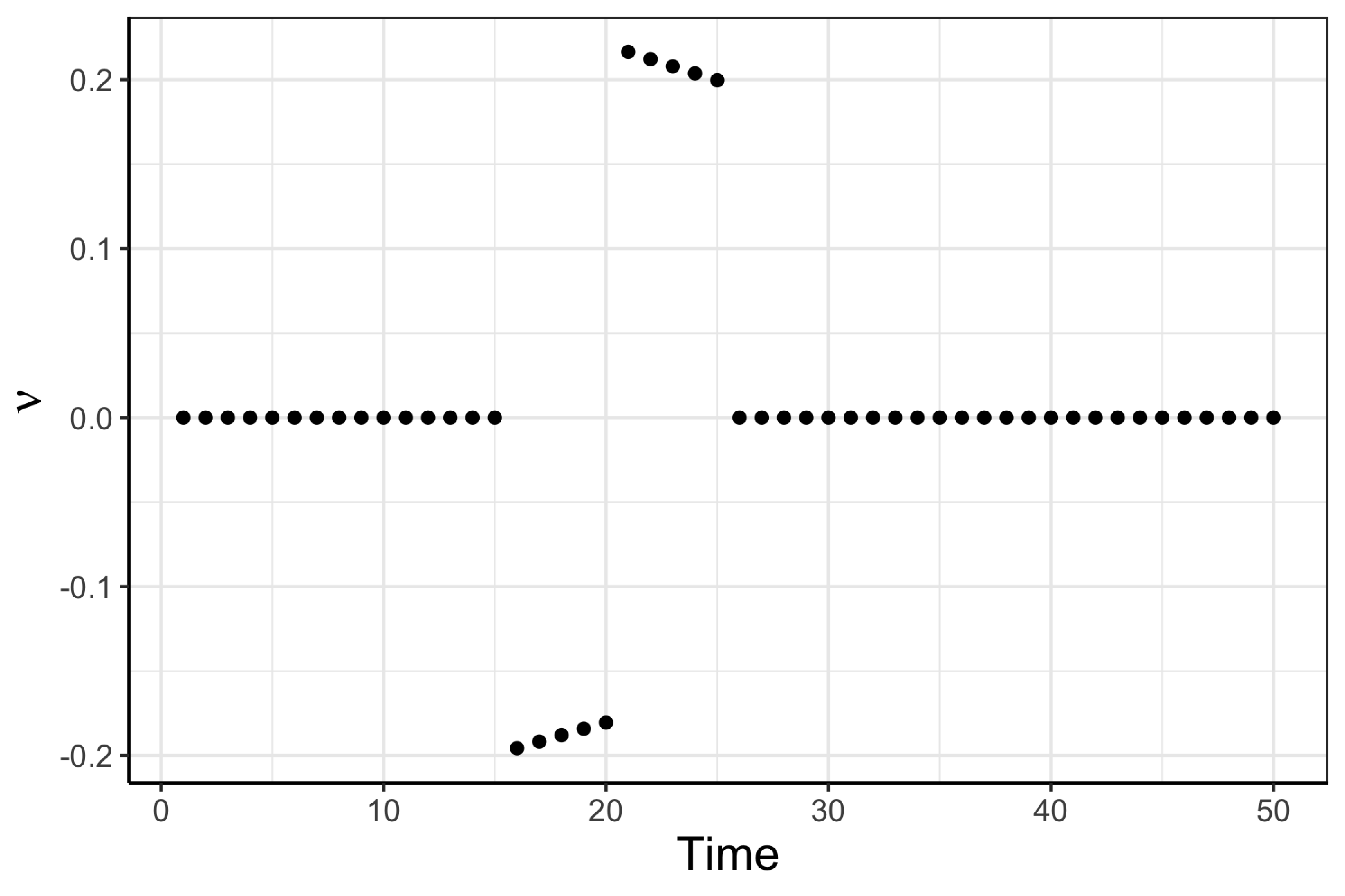
The definition (7) only applies when τ^j−h+1≥1\hat{\tau}_{j}-h+1\geq 1 and τ^j+h≤T\hat{\tau}_{j}+h\leq T. In the case that τ^j−h+1<1\hat{\tau}_{j}-h+1<1 or τ^j+h>T\hat{\tau}_{j}+h>T, we define the contrast vector ν\nu as follows:

νt\displaystyle\nu_{t} ={−γγ2−1γ2−γ2​(τ^L−τ^j)⋅γt−τ^j,τ^L≤t≤τ^jγ2−1γ2​(τ^R−τ^j)−1⋅γt−(τ^j+1),τ^j+1≤t≤τ^R0,otherwise,\displaystyle=\begin{cases}-\gamma\frac{\gamma^{2}-1}{\gamma^{2}-\gamma^{2(\hat{\tau}_{L}-\hat{\tau}_{j})}}\cdot\gamma^{t-\hat{\tau}_{j}},&\hat{\tau}_{L}\leq t\leq\hat{\tau}_{j}\\ \frac{\gamma^{2}-1}{\gamma^{2(\hat{\tau}_{R}-\hat{\tau}_{j})}-1}\cdot\gamma^{t-(\hat{\tau}_{j}+1)},&\hat{\tau}_{j}+1\leq t\leq\hat{\tau}_{R}\\ 0,&\text{otherwise}\\ \end{cases}, (39)

where τ^L=max⁡(1,τ^j−h+1)\hat{\tau}_{L}=\max(1,\hat{\tau}_{j}-h+1), and τ^R=min⁡(T,τ^j+h)\hat{\tau}_{R}=\min(T,\hat{\tau}_{j}+h).

In Figure 7, we plot the contrast vector in (7), generated with T=50T=50, γ=0.98\gamma=0.98, τ^j=20\hat{\tau}_{j}=20, and h=5h=5.

.6 Proof of Proposition 3.2

Recall that the ℓ0\ell_{0} problem (14) is equivalent to the changepoint detection problem (15), in the sense that (14) results in an estimated changepoint at τ^j\hat{\tau}_{j} if and only if τ^j\hat{\tau}_{j} is in the solution to (15).

We first prove that C⁡(ϕ)C(\phi) defined in (18) equals the objective of (15) applied to data y′​(ϕ)y^{\prime}(\phi), subject to the constraint that τ^j\hat{\tau}_{j} is in the solution.

C⁡(ϕ)\displaystyle C(\phi) =minα≥0{Cost(y1:τ^j′(ϕ),α;γ)}+minα≥0{Cost(yT:(τ^j+1)′(ϕ),α;1/γ)}+λ\displaystyle=\min_{\alpha\geq 0}\quantity{\cost\left(y_{1:\thj}'(\phi),\alpha;\gamma\right)}+\min_{\alpha\geq 0}\quantity{\cost\qty(y_{T:(\thj+1)}'(\phi),\alpha;1/\gamma)}+\lambda
=a.minα≥0{Cost(y1:τ^j′(ϕ),α;γ)}+minα≥0{Cost(y(τ^j+1):T′(ϕ),α;γ)}+λ\displaystyle\overset{a.}{=}\min_{\alpha\geq 0}\quantity{\cost\qty(y_{1:\thj}'(\phi),\alpha;\gamma)}+\min_{\alpha\geq 0}\quantity{\cost\qty(y_{(\thj+1):T}'(\phi),\alpha;\gamma)}+\lambda
=b.​min0=τ0<τ1<…<τk<τk+1=τ^j,k​{∑j=0kminα≥0⁡(12​∑t=τj+1τj+1(yt′​(ϕ)−α​γt−τj+1)2)+λ​k}\displaystyle\overset{b.}{=}\min_{\begin{subarray}{c}0=\tau_{0}<\tau_{1}<\ldots<\tau_{k}<\tau_{k+1}=\hat{\tau}_{j},k\end{subarray}}\quantity{ \sum_{j=0}^k \min_{\alpha\geq 0} \qty(\frac{1}{2} \sum_{t=\tau_j+1}^{\tau_{j+1}} \qty(y_t'(\phi)-\alpha\gamma^{t-\tau_{j+1}})^2 ) +\lambda k }
+minτ^j=τ~0<τ~1<…<τ~l<τ~l+1=T,l⁡{∑j=0lminα≥0⁡(12​∑t=τ~j+1τ~j+1(yt′​(ϕ)−α​γt−τ~j+1)2)+λ​l}+λ\displaystyle+\min_{\begin{subarray}{c}\hat{\tau}_{j}=\tilde{\tau}_{0}<\tilde{\tau}_{1}<\ldots<\tilde{\tau}_{l}<\tilde{\tau}_{l+1}=T,l\end{subarray}}\quantity{\sum_{j=0}^l \min_{\alpha\geq 0} \qty(\frac{1}{2} \sum_{t=\tilde{\tau}_{j}+1}^{\tilde{\tau}_{j+1}} \qty(y_{t}'(\phi)-\alpha\gamma^{t-\tilde{\tau}_{j+1}})^2 ) +\lambda l }+\lambda
=c.min0=τ0<τ1<…<τk<τk+1=τ^j,k,τ^j=τ~0<τ~1<…<τ~l<τ~l+1=T,l\bBigg@4{∑j=0kminα≥0(12​∑t=τj+1τj+1(yt′​(ϕ)−α​γt−τj+1)2)\displaystyle\overset{c.}{=}\min_{\begin{subarray}{c}0=\tau_{0}<\tau_{1}<\ldots<\tau_{k}<\tau_{k+1}=\hat{\tau}_{j},k,\\ \hat{\tau}_{j}=\tilde{\tau}_{0}<\tilde{\tau}_{1}<\ldots<\tilde{\tau}_{l}<\tilde{\tau}_{l+1}=T,l\end{subarray}}\bBigg@{4}\{\sum_{j=0}^{k}\min_{\alpha\geq 0}\quantity(\frac{1}{2} \sum_{t=\tau_j+1}^{\tau_{j+1}} \qty(y_t'(\phi)-\alpha\gamma^{t-\tau_{j+1}})^2 )
+∑j=0lminα≥0(12​∑t=τ~j+1τ~j+1(yt′​(ϕ)−α​γt−τ~j+1)2)+λ(k+l)\bBigg@4}+λ\displaystyle+\sum_{j=0}^{l}\min_{\alpha\geq 0}\quantity(\frac{1}{2} \sum_{t=\tilde{\tau}_{j}+1}^{\tilde{\tau}_{j+1}} \qty(y_{t}'(\phi)-\alpha\gamma^{t-\tilde{\tau}_{j+1}})^2 )+\lambda(k+l)\bBigg@{4}\}+\lambda
=d.​min0=τ0<τ1<…<τk<τk+1=T,k,τ^j∈{τ1,…,τk}​{∑j=0kminα≥0⁡(12​∑t=τj+1τj+1(yt′​(ϕ)−α​γt−τj+1)2)+λ​k}.\displaystyle\overset{d.}{=}\min_{\begin{subarray}{c}0=\tau_{0}<\tau_{1}<\ldots<\tau_{k}<\tau_{k+1}=T,\\ k,\hat{\tau}_{j}\in\{\tau_{1},\ldots,\tau_{k}\}\end{subarray}}\quantity{ \sum_{j=0}^k \min_{\alpha\geq 0} \qty(\frac{1}{2} \sum_{t=\tau_j+1}^{\tau_{j+1}} \qty(y_t'(\phi)-\alpha\gamma^{t-\tau_{j+1}})^2 ) +\lambda k }.

Here, a.a. follows from Lemma .5 and b.b. follows from Lemma .3. Part c.c. follows from combining the two minimization problems, and finally part d.d. follows from treating (k+l)(k+l) as a new variable in the optimization problem.

Next, we show that C′​(ϕ)C^{\prime}(\phi) defined in (19) equals the objective of (15) applied to data y′​(ϕ)y^{\prime}(\phi), subject to the constraint that τ^j\hat{\tau}_{j} is not in the solution.

C′​(ϕ)\displaystyle C^{\prime}(\phi) =minα≥0{Cost(y1:τ^j′(ϕ),α;γ)+Cost(yT:(τ^j+1)′(ϕ),γα;1/γ)}\displaystyle=\min_{\alpha\geq 0}\quantity{ \cost\qty(y_{1:\thj}'(\phi),\alpha;\gamma) + \cost\qty(y_{T:(\thj+1)}'(\phi),\gamma\alpha;1/\gamma)}
=a.minα≥0\bBigg@4{min0=τ0<τ1<…<τk<τk+1=τ^j,α0,…,αk−1≥0,αk=α,k{12​∑j=0k∑t=τj+1τj+1(yt′​(ϕ)−αj​γt−τj+1)2+λ​k}\displaystyle\overset{a.}{=}\min_{\alpha\geq 0}\bBigg@{4}\{\min_{\begin{subarray}{c}0=\tau_{0}<\tau_{1}<\ldots<\tau_{k}<\tau_{k+1}=\hat{\tau}_{j},\\ \alpha_{0},\ldots,\alpha_{k-1}\geq 0,\alpha_{k}=\alpha,k\end{subarray}}\quantity{ \frac{1}{2} \sum_{j=0}^k \sum_{t=\tau_j+1}^{\tau_{j+1}} \qty(y_t'(\phi)-\alpha_j \gamma^{t-\tau_{j+1}})^2 +\lambda k }
+minτ^j=τ0<τ1<…<τk<τk+1=T,α0,…,αk≥0,αk=γ​α,k{12​∑j=0k∑t=τj+1τj+1(yT+τ^j+1−t′​(ϕ)−αj​(1/γ)t−τj+1)2+λ​k}\bBigg@4}\displaystyle+\min_{\begin{subarray}{c}\hat{\tau}_{j}=\tau_{0}<\tau_{1}<\ldots<\tau_{k}<\tau_{k+1}=T,\\ \alpha_{0},\ldots,\alpha_{k}\geq 0,\alpha_{k}=\gamma\alpha,k\end{subarray}}\quantity{\frac{1}{2} \sum_{j=0}^k \sum_{t=\tau_j+1}^{\tau_{j+1}} \qty(y_{T+\thj+1-t}'(\phi)-\alpha_j (1/\gamma)^{t-\tau_{j+1}})^2 +\lambda k }\bBigg@{4}\}
=b.minα≥0\bBigg@4{min0=τ0<τ1<…<τk<τk+1=τ^j,α0,…,αk−1≥0,αk=α,k{12​∑j=0k∑t=τj+1τj+1(yt′​(ϕ)−αj​γt−τj+1)2+λ​k}\displaystyle\overset{b.}{=}\min_{\alpha\geq 0}\bBigg@{4}\{\min_{\begin{subarray}{c}0=\tau_{0}<\tau_{1}<\ldots<\tau_{k}<\tau_{k+1}=\hat{\tau}_{j},\\ \alpha_{0},\ldots,\alpha_{k-1}\geq 0,\alpha_{k}=\alpha,k\end{subarray}}\quantity{ \frac{1}{2} \sum_{j=0}^k \sum_{t=\tau_j+1}^{\tau_{j+1}} \qty(y_t'(\phi)-\alpha_j \gamma^{t-\tau_{j+1}})^2 +\lambda k }
+minT=τ~0>τ~1>…>τ~k>τ~k+1=τ^j,α0,…,αk≥0,αk=γ​α,k{12​∑j=0k∑t=τ~j+1τ~j+1(yt′​(ϕ)−αj​γt−τ~j+1)2+λ​k}\bBigg@4}\displaystyle+\min_{\begin{subarray}{c}T=\tilde{\tau}_{0}>\tilde{\tau}_{1}>\ldots>\tilde{\tau}_{k}>\tilde{\tau}_{k+1}=\hat{\tau}_{j},\\ \alpha_{0},\ldots,\alpha_{k}\geq 0,\alpha_{k}=\gamma\alpha,k\end{subarray}}\quantity{\frac{1}{2} \sum_{j=0}^k \sum_{t=\tilde{\tau}_{j+1}}^{\tilde{\tau}_{j}+1} \qty(y_{t}'(\phi)- \alpha_j \gamma^{t-\tilde{\tau}_{j+1}})^2 +\lambda k }\bBigg@{4}\}
=c.​min0=τ0<τ1<…<τk<τk+1=τ^j,α0,…,αk−1≥0,αk=α,k,τ^j=τ~k~+1<τ~k~<…<τ~1<τ~0=Tα~0,…,α~k~≥0,α~k~=γ​α,k~​{12​∑j=0k∑t=τj+1τj+1(yt′​(ϕ)−αj​γt−τj+1)2+λ​k+12​∑j=0k~∑t=τ~j+1τ~j+1(yt′​(ϕ)−α~j​γt−τ~j+1)2+λ​k~}\displaystyle\overset{c.}{=}\min_{\begin{subarray}{c}0=\tau_{0}<\tau_{1}<\ldots<\tau_{k}<\tau_{k+1}=\hat{\tau}_{j},\\ \alpha_{0},\ldots,\alpha_{k-1}\geq 0,\alpha_{k}=\alpha,k,\\ \hat{\tau}_{j}=\tilde{\tau}_{\tilde{k}+1}<\tilde{\tau}_{\tilde{k}}<\ldots<\tilde{\tau}_{1}<\tilde{\tau}_{0}=T\,\\ \tilde{\alpha}_{0},\ldots,\tilde{\alpha}_{\tilde{k}}\geq 0,\tilde{\alpha}_{\tilde{k}}=\gamma\alpha,\tilde{k}\end{subarray}}\left\{\frac{1}{2}\sum_{j=0}^{k}\sum_{t=\tau_{j}+1}^{\tau_{j+1}}\quantity(y_t'(\phi)-\alpha_j \gamma^{t-\tau_{j+1}})^{2}+\lambda k+\frac{1}{2}\sum_{j=0}^{\tilde{k}}\sum_{t=\tilde{\tau}_{j}+1}^{\tilde{\tau}_{j+1}}\quantity(y_{t}'(\phi)- \tilde{\alpha}_j \gamma^{t-\tilde{\tau}_{j+1}})^{2}+\lambda\tilde{k}\right\}
=d.​min0=τ0<τ1<…<τk<τk+1=T,α0,…,αk≥0,k,τ^j≠τj,∀j=1,…,k.​{12​∑j=0k∑t=τj+1τj+1(yt′​(ϕ)−αj​γt−τj+1)2+λ​k}\displaystyle\overset{d.}{=}\min_{\begin{subarray}{c}0=\tau_{0}<\tau_{1}<\ldots<\tau_{k}<\tau_{k+1}=T,\\ \alpha_{0},\ldots,\alpha_{k}\geq 0,k,\\ \hat{\tau}_{j}\neq\tau_{j},\forall j=1,\ldots,k.\end{subarray}}\left\{\frac{1}{2}\sum_{j=0}^{k}\sum_{t=\tau_{j}+1}^{\tau_{j+1}}\quantity(y_t'(\phi)-\alpha_j \gamma^{t-\tau_{j+1}})^{2}+\lambda k\right\}
=e.​min0=τ0<τ1<…<τk<τk+1=T,k,τ^j∉{τ1,…,τk}​{∑j=0kminα≥0⁡(12​∑t=τj+1τj+1(yt′​(ϕ)−α​γt−τj+1)2)+λ​k}.\displaystyle\overset{e.}{=}\min_{\begin{subarray}{c}0=\tau_{0}<\tau_{1}<\ldots<\tau_{k}<\tau_{k+1}=T,\\ k,\hat{\tau}_{j}\notin\{\tau_{1},\ldots,\tau_{k}\}\end{subarray}}\quantity{ \sum_{j=0}^k \min_{\alpha\geq 0} \qty(\frac{1}{2} \sum_{t=\tau_j+1}^{\tau_{j+1}} \qty(y_t'(\phi)-\alpha\gamma^{t-\tau_{j+1}})^2 ) +\lambda k }.

Part a.a. follows from expanding Cost​(⋅)\text{Cost}(\cdot) using Lemma .1. We then change the optimization variable in the second term from τj\tau_{j} to τ~j=T+τ^j−τj\tilde{\tau}_{j}=T+\hat{\tau}_{j}-\tau_{j}, which does not change the optimization problem because the mapping between τ~j\tilde{\tau}_{j} and τj\tau_{j} is invertible; re-indexing the summation completes part b.b. Next, c.c. follows from combining the two optimization problems. In step d.d., we observe that the two constraints αk=α\alpha_{k}=\alpha (i.e., fitted value at timepoint τ^j\hat{\tau}_{j} is α\alpha) and α~k~=γ​α\tilde{\alpha}_{\tilde{k}}=\gamma\alpha (i.e., fitted value at timepoint τ^j+1\hat{\tau}_{j}+1 is γ​α\gamma\alpha) are equivalent to a single constraint that τ^j\hat{\tau}_{j} is not a changepoint. Finally, step e.e. follows from pulling the optimization over αj\alpha_{j} inside the summation.

To summarize, we have proven that

C⁡(ϕ)\displaystyle C(\phi) =min0=τ0<τ1<…<τk<τk+1=T,k,τ^j∈{τ1,…,τk}⁡{∑j=0kminα≥0⁡(12​∑t=τj+1τj+1(yt′​(ϕ)−α​γt−τj+1)2)+λ​k},\displaystyle=\min_{\begin{subarray}{c}0=\tau_{0}<\tau_{1}<\ldots<\tau_{k}<\tau_{k+1}=T,\\ k,\hat{\tau}_{j}\in\{\tau_{1},\ldots,\tau_{k}\}\end{subarray}}\quantity{ \sum_{j=0}^k \min_{\alpha\geq 0} \qty(\frac{1}{2} \sum_{t=\tau_j+1}^{\tau_{j+1}} \qty(y_t'(\phi)-\alpha\gamma^{t-\tau_{j+1}})^2 ) +\lambda k }, (40)

and

C′​(ϕ)\displaystyle C^{\prime}(\phi) =min0=τ0<τ1<…<τk<τk+1=T,k,τ^j∉{τ1,…,τk}⁡{∑j=0kminα≥0⁡(12​∑t=τj+1τj+1(yt′​(ϕ)−α​γt−τj+1)2)+λ​k}.\displaystyle=\min_{\begin{subarray}{c}0=\tau_{0}<\tau_{1}<\ldots<\tau_{k}<\tau_{k+1}=T,\\ k,\hat{\tau}_{j}\notin\{\tau_{1},\ldots,\tau_{k}\}\end{subarray}}\quantity{ \sum_{j=0}^k \min_{\alpha\geq 0} \qty(\frac{1}{2} \sum_{t=\tau_j+1}^{\tau_{j+1}} \qty(y_t'(\phi)-\alpha\gamma^{t-\tau_{j+1}})^2 ) +\lambda k }. (41)

By inspection of (40) and (41), we conclude that {ϕ:C⁡(ϕ)≤C′​(ϕ)}={ϕ:τ^j∈ℳ​(y′​(ϕ))}\left\{\phi:C(\phi)\leq C^{\prime}(\phi)\right\}=\left\{\phi:\hat{\tau}_{j}\in\mathscr{M}\quantity(y'\qty(\phi))\right\}, which completes the proof.

We present the technical lemmas used in the proof below.

Lemma .1.

For Cost(y1:s,α;γ)\text{Cost}\quantity(y_{1:s},\alpha;\gamma) defined in (16), we have

Cost(y1:s,α;γ)=min0=τ0<τ1<…<τk<τk+1=s,α0,…,αk≥0,αk=α,k{12​∑j=0k∑t=τj+1τj+1(yt−αj​γt−τj+1)2+λ​k}.\text{Cost}\quantity(y_{1:s},\alpha;\gamma)=\min_{\begin{subarray}{c}0=\tau_{0}<\tau_{1}<\ldots<\tau_{k}<\tau_{k+1}=s,\\ \alpha_{0},\ldots,\alpha_{k}\geq 0,\alpha_{k}=\alpha,k\end{subarray}}\quantity{\frac{1}{2}\sum_{j=0}^k\sum_{t=\tau_j+1}^{\tau_{j+1}} \qty(y_t-\alpha_j \gamma^{t-\tau_{j+1}})^2 + \lambda k}. (42)
Proof .2.
Cost(y1:s,α;γ)\displaystyle\text{Cost}(y_{1:s},\alpha;\gamma) =a.​min0≤τ<s​{F⁡(τ)+12​(∑t=τ+1s(yt−α​γt−s)2)+λ}\displaystyle\overset{a.}{=}\min_{0\leq\tau<s}\quantity{ F(\tau) + \frac{1}{2} \left( \sum_{t=\tau+1}^s (y_t - \alpha\gamma^{t-s})^2 \right) + \lambda}
=b.min0≤τ<s{min0=τ0<τ1<…<τk<τk+1=τ,k12(∑j=0kminα≥0{∑t=τj+1τj+1(yt−α​γt−τj+1)2}+λk)\displaystyle\overset{b.}{=}\min_{0\leq\tau<s}\Bigg\{\min_{0=\tau_{0}<\tau_{1}<\ldots<\tau_{k}<\tau_{k+1}=\tau,k}\frac{1}{2}\left(\sum_{j=0}^{k}\min_{\alpha\geq 0}\left\{\sum_{t=\tau_{j}+1}^{\tau_{j+1}}\quantity(y_t-\alpha\gamma^{t-\tau_{j+1}})^{2}\right\}+\lambda k\right)
+12(∑t=τ+1s(yt−α​γt−s)2)+λ}\displaystyle+\frac{1}{2}\left(\sum_{t=\tau+1}^{s}\quantity(y_t - \alpha\gamma^{t-s})^{2}\right)+\lambda\Bigg\}
=c.​min0=τ0<τ1<…<τk<τk+1=τ<s,α0,…,αk≥0,k,τ​{12​∑j=0k∑t=τj+1τj+1(yt−αj​γt−τj+1)2+λ​k+12​∑t=τk+1+1s(yt−α​γt−s)2+λ}\displaystyle\overset{c.}{=}\min_{\begin{subarray}{c}0=\tau_{0}<\tau_{1}<\ldots<\tau_{k}<\tau_{k+1}=\tau<s,\\ \alpha_{0},\ldots,\alpha_{k}\geq 0,k,\tau\end{subarray}}\quantity{ \frac{1}{2} \sum_{j=0}^k \sum_{t=\tau_j+1}^{\tau_{j+1}} \qty(y_t-\alpha_j \gamma^{t-\tau_{j+1}})^2 + \lambda k + \frac{1}{2}\sum_{t=\tau_{k+1}+1}^s \qty(y_t-\alpha\gamma^{t-s})^2 + \lambda}
=d.​min0=τ0<τ1<…<τk<τk+1=s,α0,…,αk≥0,αk=α,k​{12​∑j=0k∑t=τj+1τj+1(yt−αj​γt−τj+1)2+λ​k}.\displaystyle\overset{d.}{=}\min_{\begin{subarray}{c}0=\tau_{0}<\tau_{1}<\ldots<\tau_{k}<\tau_{k+1}=s,\\ \alpha_{0},\ldots,\alpha_{k}\geq 0,\alpha_{k}=\alpha,k\end{subarray}}\quantity{\frac{1}{2}\sum_{j=0}^k\sum_{t=\tau_j+1}^{\tau_{j+1}} \qty(y_t-\alpha_j \gamma^{t-\tau_{j+1}})^2 + \lambda k}.

Here, a.a. follows from the definition in (16) and b.b. follows from the definition of F⁡(τ)F(\tau), the optimal cost of segmenting the first τ\tau data points. Part c.c. follows from pulling the minα≥0\min_{\alpha\geq 0} operation out of the summation, which is performed separately for each data segment y(τj+1):τj+1y_{(\tau_{j}+1):\tau_{j+1}}. Finally, part d.d. follows by inspection.

Lemma .3.

For Cost(y1:s,α;γ)\text{Cost}\quantity(y_{1:s},\alpha;\gamma) defined in (16), we have

minα≥0{Cost(y1:s,α;γ)}=min0=τ0<τ1<…<τk<τk+1=s,k{∑j=0kminα≥0⁡{12​∑t=τj+1τj+1(yt−α​γt−τj+1)2}+λ​k}.\min_{\alpha\geq 0}\quantity{\cost\qty(y_{1:s},\alpha;\gamma)}=\min_{0=\tau_{0}<\tau_{1}<\ldots<\tau_{k}<\tau_{k+1}=s,k}\quantity{\sum_{j=0}^k \min_{\alpha\geq 0} \left\{\frac{1}{2} \sum_{t=\tau_j+1}^{\tau_{j+1}} \qty(y_t-\alpha\gamma^{t-\tau_{j+1}})^2 \right\} +\lambda k}.
Proof .4.
minα≥0{Cost(y1:s,α;γ)}\displaystyle\min_{\alpha\geq 0}\quantity{\cost\qty(y_{1:s},\alpha;\gamma)} =a.​minα≥0​{min0=τ0<τ1<…<τk<τk+1=s,α0,…,αk≥0,αk=α,k⁡{12​∑j=0k∑t=τj+1τj+1(yt−αj​γt−τj+1)2+λ​k}}\displaystyle\overset{a.}{=}\min_{\alpha\geq 0}\quantity{\min_{\substack{0=\tau_0<\tau_1<\ldots<\tau_k<\tau_{k+1}=s, \\ \alpha_0,\ldots,\alpha_k\geq 0, \alpha_k = \alpha, k}} \qty{\frac{1}{2}\sum_{j=0}^k\sum_{t=\tau_j+1}^{\tau_{j+1}} \qty(y_t-\alpha_j \gamma^{t-\tau_{j+1}})^2 + \lambda k}}
=min0=τ0<τ1<…<τk<τk+1=s,α0,…,αk≥0,k⁡{12​∑j=0k∑t=τj+1τj+1(yt−αj​γt−τj+1)2+λ​k}\displaystyle=\min_{\begin{subarray}{c}0=\tau_{0}<\tau_{1}<\ldots<\tau_{k}<\tau_{k+1}=s,\\ \alpha_{0},\ldots,\alpha_{k}\geq 0,k\end{subarray}}\quantity{\frac{1}{2}\sum_{j=0}^k\sum_{t=\tau_j+1}^{\tau_{j+1}} \qty(y_t-\alpha_j \gamma^{t-\tau_{j+1}})^2 + \lambda k}
=b.​min0=τ0<τ1<…<τk<τk+1=s,k​{12​∑j=0kminα≥0⁡{12​∑t=τj+1τj+1(yt−α​γt−τj+1)2}+λ​k}.\displaystyle\overset{b.}{=}\min_{\begin{subarray}{c}0=\tau_{0}<\tau_{1}<\ldots<\tau_{k}<\tau_{k+1}=s,k\end{subarray}}\quantity{\frac{1}{2}\sum_{j=0}^k \min_{\alpha\geq 0}\qty{ \frac{1}{2} \sum_{t=\tau_j+1}^{\tau_{j+1}} \qty(y_t-\alpha\gamma^{t-\tau_{j+1}})^2 }+ \lambda k}.

Here, a.a. follows from Lemma .1. b.b. follows from noting that αj\alpha_{j} can be minimized independently for each data segment y(τ^j+1):τ^j+1y_{(\hat{\tau}_{j}+1):\hat{\tau}_{j+1}}.

Lemma .5.

For Cost(y1:s,α;γ)\text{Cost}\quantity(y_{1:s},\alpha;\gamma) defined in (16), we have

minα≥0{Cost(y1:s,α;γ)}=minα≥0{Cost(ys:1,α;1/γ)}.\min_{\alpha\geq 0}\quantity{\cost\qty(y_{1:s},\alpha;\gamma)}=\min_{\alpha\geq 0}\quantity{\cost\qty(y_{s:1},\alpha;1/\gamma)}.
Proof .6.
minα≥0{Cost(y1:s,α;γ)}\displaystyle\min_{\alpha\geq 0}\quantity{\cost\qty(y_{1:s},\alpha;\gamma)} =a.​min0=τ0<τ1<…<τk<τk+1=s,α0,…,αk≥0,k​{12​∑j=0k∑t=τj+1τj+1(yt−αj​γt−τj+1)2+λ​k}\displaystyle\overset{a.}{=}\min_{\begin{subarray}{c}0=\tau_{0}<\tau_{1}<\ldots<\tau_{k}<\tau_{k+1}=s,\\ \alpha_{0},\ldots,\alpha_{k}\geq 0,k\end{subarray}}\quantity{\frac{1}{2}\sum_{j=0}^k\sum_{t=\tau_j+1}^{\tau_{j+1}} \qty(y_t-\alpha_j \gamma^{t-\tau_{j+1}})^2 + \lambda k}
=b.​mins=τ~0>τ~1>…>τ~k>τ~k+1=0,α0,…,αk≥0,k​{12​∑j=0k∑t=s−τ~j+1s−τ~j+1(yt−αj​γt−(s−τ~j+1))2+λ​k}\displaystyle\overset{b.}{=}\min_{\begin{subarray}{c}s=\tilde{\tau}_{0}>\tilde{\tau}_{1}>\ldots>\tilde{\tau}_{k}>\tilde{\tau}_{k+1}=0,\\ \alpha_{0},\ldots,\alpha_{k}\geq 0,k\end{subarray}}\quantity{\frac{1}{2}\sum_{j=0}^k\sum_{t=s-\tilde{\tau}_j+1}^{s-\tilde{\tau}_{j+1}} \qty(y_t-\alpha_j \gamma^{t-(s-\tilde{\tau}_{j+1})})^2 + \lambda k}
=c.​mins=τ~0>τ~1>…>τ~k>τ~k+1=0,α0,…,αk≥0,k​{12​∑j=0k∑t=τ~j+1τ~j(ys−t−αj​(1/γ)t−τ~j+1)2+λ​k}\displaystyle\overset{c.}{=}\min_{\begin{subarray}{c}s=\tilde{\tau}_{0}>\tilde{\tau}_{1}>\ldots>\tilde{\tau}_{k}>\tilde{\tau}_{k+1}=0,\\ \alpha_{0},\ldots,\alpha_{k}\geq 0,k\end{subarray}}\quantity{\frac{1}{2}\sum_{j=0}^k\sum_{t=\tilde{\tau}_{j+1}}^{\tilde{\tau}_{j}} \qty(y_{s-t}-\alpha_j (1/\gamma)^{t-\tilde{\tau}_{j+1}})^2 + \lambda k}
=d.minα≥0{Cost(ys:1,α;1/γ)}.\displaystyle\overset{d.}{=}\min_{\alpha\geq 0}\quantity{\cost\qty(y_{s:1},\alpha;1/\gamma)}.

Part a.a. follows from Lemma .1. In step b.b., we change the optimization variable from τj\tau_{j} to τ~j=s−τj\tilde{\tau}_{j}=s-\tau_{j}, which does not change the optimization problem because the mapping between τ~j\tilde{\tau}_{j} and τj\tau_{j} is invertible. Step c.c. follows from re-indexing the summation, and finally d.d. follows from Lemma .1 again.

.7 Proof of Proposition 3.3

To begin, we will prove (21) using an induction argument. The following claim serves as the “base case” for the recursion.

Lemma .7.
Cost(y1:(τ^j−h+1)′(ϕ),α;γ)=minf∈𝒞τ^j−h+1f(α,ϕ),\text{Cost}\left(y_{1:(\hat{\tau}_{j}-h+1)}^{\prime}(\phi),\alpha;\gamma\right)=\min_{f\in\mathscr{C}_{\hat{\tau}_{j}-h+1}}f(\alpha,\phi), (43)

where

𝒞τ^j−h+1={Cost(y1:(τ^j−h)′(ϕ),α/γ;γ)+12(yτ^j−h+1′(ϕ)−α)2,\displaystyle\mathscr{C}_{\hat{\tau}_{j}-h+1}=\Bigg\{\text{Cost}\left(y_{1:(\hat{\tau}_{j}-h)}^{\prime}(\phi),\alpha/\gamma;\gamma\right)+\frac{1}{2}\left(y_{\hat{\tau}_{j}-h+1}^{\prime}(\phi)-\alpha\right)^{2},
minα′≥0{Cost(y1:(τ^j−h)′(ϕ),α′;γ)}+λ+12(yτ^j−h+1′(ϕ)−α)2}.\displaystyle\min_{\alpha^{\prime}\geq 0}\quantity{\cost\left(y_{1:(\thj-h)}'(\phi),\alpha';\gamma\right)}+\lambda+\frac{1}{2}\left(y_{\hat{\tau}_{j}-h+1}^{\prime}(\phi)-\alpha\right)^{2}\Bigg\}. (44)
Proof .8.

To prove Lemma .7, we will first compute Cost(y1:(τ^j−h+1)′(ϕ),α;γ)\text{Cost}\left(y_{1:(\hat{\tau}_{j}-h+1)}^{\prime}(\phi),\alpha;\gamma\right) using the definition in (16); we will then show that this equals minf∈𝒞τ^j−h+1⁡f⁡(α,ϕ)\min_{f\in\mathscr{C}_{\hat{\tau}_{j}-h+1}}f(\alpha,\phi), with 𝒞τ^j−h+1\mathscr{C}_{\hat{\tau}_{j}-h+1} in (44).

Per the definition of ν\nu in (7), y1:(τ^j−h)′(ϕ)=y1:(τ^j−h)y^{\prime}_{1:(\hat{\tau}_{j}-h)}(\phi)=y_{1:(\hat{\tau}_{j}-h)}; therefore, 𝒞τ^j−h=Cost(y1:(τ^j−h)′(ϕ),α;γ)=Cost(y1:(τ^j−h),α;γ)\mathscr{C}_{\hat{\tau}_{j}-h}=\text{Cost}\left(y_{1:(\hat{\tau}_{j}-h)}^{\prime}(\phi),\alpha;\gamma\right)=\text{Cost}\left(y_{1:(\hat{\tau}_{j}-h)},\alpha;\gamma\right). From Proposition 3.1, this means that 𝒞τ^j−h\mathscr{C}_{\hat{\tau}_{j}-h} is a piecewise quadratic function of α\alpha only.

Now we consider the function Cost(y1:(τ^j−h+1)′(ϕ),α;γ)\text{Cost}\left(y_{1:(\hat{\tau}_{j}-h+1)}^{\prime}(\phi),\alpha;\gamma\right). There are two possibilities:

  1. 1.

    There is no changepoint at the (τ^j−h)(\hat{\tau}_{j}-h)th time step. In this case, Cost(y1:(τ^j−h+1)′(ϕ),α;γ)\text{Cost}\left(y_{1:(\hat{\tau}_{j}-h+1)}^{\prime}\left(\phi\right),\alpha;\gamma\right) equals

    Cost(y1:(τ^j−h)′(ϕ),α/γ;γ)+12(yτ^j−h+1′(ϕ)−α)2,\displaystyle\text{Cost}\left(y_{1:(\hat{\tau}_{j}-h)}^{\prime}(\phi),\alpha/\gamma;\gamma\right)+\frac{1}{2}\left(y_{\hat{\tau}_{j}-h+1}^{\prime}\quantity(\phi)-\alpha\right)^{2},

    where α/γ\alpha/\gamma accounts for the exponential calcium decay.

  2. 2.

    There is a changepoint at the (τ^j−h)(\hat{\tau}_{j}-h)th time step. In this case, Cost(y1:(τ^j−h+1)′(ϕ),α;γ)\text{Cost}\left(y_{1:(\hat{\tau}_{j}-h+1)}^{\prime}(\phi),\alpha;\gamma\right) equals

    minα′≥0{Cost(y1:(τ^j−h)′(ϕ),α′;γ)}+λ+12(yτ^j−h+1′(ϕ)−α)2,\displaystyle\min_{\alpha^{\prime}\geq 0}\quantity{\cost\left(y_{1:(\thj-h)}'(\phi),\alpha';\gamma\right)}+\lambda+\frac{1}{2}\left(y_{\hat{\tau}_{j}-h+1}^{\prime}(\phi)-\alpha\right)^{2},

    where the changepoint incurs a penalty of λ\lambda, and there can be an arbitrary change in the calcium from timepoint τ^j−h\hat{\tau}_{j}-h to τ^j−h+1\hat{\tau}_{j}-h+1.

Therefore,

Cost(y1:(τ^j−h+1)′(ϕ),α;γ)=\displaystyle\text{Cost}\left(y_{1:(\hat{\tau}_{j}-h+1)}^{\prime}(\phi),\alpha;\gamma\right)= min{Cost(y1:(τ^j−h)′(ϕ),α/γ;γ)+12(yτ^j−h+1′(ϕ)−α)2,\displaystyle\min\Bigg\{\text{Cost}\left(y_{1:(\hat{\tau}_{j}-h)}^{\prime}(\phi),\alpha/\gamma;\gamma\right)+\frac{1}{2}\left(y_{\hat{\tau}_{j}-h+1}^{\prime}(\phi)-\alpha\right)^{2},
minα′≥0{Cost(y1:(τ^j−h)′(ϕ),α′;γ)}+λ+12(yτ^j−h+1′(ϕ)−α)2}\displaystyle\min_{\alpha^{\prime}\geq 0}\quantity{\cost\left(y_{1:(\thj-h)}'(\phi),\alpha';\gamma\right)}+\lambda+\frac{1}{2}\left(y_{\hat{\tau}_{j}-h+1}^{\prime}(\phi)-\alpha\right)^{2}\Bigg\}
=\displaystyle= minf∈𝒞τ^j−h+1⁡f⁡(α,ϕ),\displaystyle\min_{f\in\mathscr{C}_{\hat{\tau}_{j}-h+1}}f(\alpha,\phi), (45)

where the last equality follows from (44). This completes the proof.

We will now prove the inductive step for the recursion, which relies on the following claim.

Lemma .9.

Suppose that for some s∈{τ^j−h+1,…,τ^j−1}s\in\left\{\hat{\tau}_{j}-h+1,\ldots,\hat{\tau}_{j}-1\right\},

Cost(y1:s′(ϕ),α;γ)=minf∈𝒞sf(α,ϕ).\displaystyle\text{Cost}\left(y_{1:s}^{\prime}(\phi),\alpha;\gamma\right)=\min_{f\in\mathscr{C}_{s}}f(\alpha,\phi). (46)

Then,

Cost(y1:(s+1)′(ϕ),α;γ)=minf∈𝒞s+1f(α,ϕ),\displaystyle\text{Cost}\left(y_{1:(s+1)}^{\prime}(\phi),\alpha;\gamma\right)=\min_{f\in\mathscr{C}_{s+1}}f(\alpha,\phi), (47)

where 𝒞s+1\mathscr{C}_{s+1} is defined recursively according to (23).

Proof .10.

To begin, we apply Proposition 3.1 with y′​(ϕ)y^{\prime}(\phi) instead of yy and get

Cost(y1:(s+1)′(ϕ),α;γ)=min{Cost(y1:s′(ϕ),α/γ;γ),minα′≥0Cost(y1:s′(ϕ),α′;γ)+λ}+12(ys+1′(ϕ)−α)2.\text{Cost}\left(y_{1:(s+1)}^{\prime}(\phi),\alpha;\gamma\right)=\min\left\{\text{Cost}\left(y_{1:s}^{\prime}(\phi),\alpha/\gamma;\gamma\right),\min_{\alpha^{\prime}\geq 0}\text{Cost}\left(y_{1:s}^{\prime}(\phi),\alpha^{\prime};\gamma\right)+\lambda\right\}+\frac{1}{2}\left(y_{s+1}^{\prime}(\phi)-\alpha\right)^{2}. (48)

Applying the inductive hypothesis in (46) with α/γ\alpha/\gamma instead of α\alpha, we have that

Cost(y1:s′(ϕ),α/γ;γ)=minf∈𝒞sf(α/γ,ϕ),\displaystyle\text{Cost}\left(y_{1:s}^{\prime}(\phi),\alpha/\gamma;\gamma\right)=\min_{f\in\mathscr{C}_{s}}f(\alpha/\gamma,\phi), (49)

and

minα′≥0{Cost(y1:s′(ϕ),α′;γ)}=minα′≥0{minf∈𝒞s⁡f⁡(α′,ϕ)}.\displaystyle\min_{\alpha^{\prime}\geq 0}\quantity{\cost\left(y_{1:s}'(\phi),\alpha';\gamma\right)}=\min_{\alpha^{\prime}\geq 0}\quantity{\min_{f\in\mathcal{C}_s} f(\alpha',\phi)}. (50)

Therefore,

Cost(y1:(s+1)′(ϕ),α;γ)\displaystyle\text{Cost}\left(y_{1:(s+1)}^{\prime}(\phi),\alpha;\gamma\right) =a.​min⁡{minf∈𝒞s⁡f⁡(α/γ,ϕ),minα′≥0⁡{minf∈𝒞s⁡f⁡(α′,ϕ)}+λ}+12​(ys+1′​(ϕ)−α)2\displaystyle\overset{a.}{=}\min\left\{\min_{f\in\mathscr{C}_{s}}f(\alpha/\gamma,\phi),\min_{\alpha^{\prime}\geq 0}\quantity{\min_{f\in\mathcal{C}_s} f(\alpha',\phi)}+\lambda\right\}+\frac{1}{2}\left(y_{s+1}^{\prime}(\phi)-\alpha\right)^{2} (51)
=b.​min⁡{minf∈𝒞s⁡f⁡(α/γ,ϕ)+12​(ys+1′​(ϕ)−α)2,minf∈𝒞s⁡{minα′≥0⁡{f⁡(α′,ϕ)}}+λ+12​(ys+1′​(ϕ)−α)2},\displaystyle\overset{b.}{=}\min\quantity{ \min_{f\in\mathcal{C}_s} f(\alpha/\gamma,\phi) + \frac{1}{2}\left(y_{s+1}'(\phi)-\alpha\right)^2 , \min_{f\in\mathcal{C}_s} \qty{ \min_{\alpha'\geq 0}\qty{f(\alpha',\phi)}} + \lambda+ \frac{1}{2}\left(y_{s+1}'(\phi)-\alpha\right)^2 }, (52)

where a.a. follows from (46) and (48), and b.b. follows from exchanging the order of minimization and distributing the 12​(ys+1′​(ϕ)−α)2\frac{1}{2}\left(y_{s+1}^{\prime}(\phi)-\alpha\right)^{2} term inside.

Furthermore,

minf∈𝒞s+1⁡f⁡(α,ϕ)\displaystyle\min_{f\in\mathscr{C}_{s+1}}f(\alpha,\phi) =a.​minf∈{(⋃f∈𝒞s{f⁡(α/γ,ϕ)+12​(ys+1′​(ϕ)−α)2})​⋃{gs+1​(ϕ)+12​(ys+1′​(ϕ)−α)2}}⁡f⁡(α,ϕ)\displaystyle\overset{a.}{=}\min_{f\in\quantity{\left( \bigcup_{f \in\mathcal{C}_{s}} \left\{ f(\alpha/\gamma,\phi)+\frac{1}{2}\left(y'_{s+1}(\phi)-\alpha\right)^2 \right\} \right) \bigcup\left\{ g_{s+1}(\phi)+\frac{1}{2}\left(y'_{s+1}(\phi)-\alpha\right)^2 \right\} }}f(\alpha,\phi) (53)
=b.​min⁡{minf∈𝒞s⁡{f⁡(α/γ,ϕ)+12​(ys+1′​(ϕ)−α)2},gs+1​(ϕ)+12​(ys+1′​(ϕ)−α)2}\displaystyle\overset{b.}{=}\min\quantity{ \min_{f \in\mathcal{C}_{s}} \left\{ f(\alpha/\gamma,\phi)+\frac{1}{2}\left(y'_{s+1}(\phi)-\alpha\right)^2 \right\}, g_{s+1}(\phi)+\frac{1}{2}\left(y'_{s+1}(\phi)-\alpha\right)^2 } (54)
=c.​min⁡{minf∈𝒞s⁡{f⁡(α/γ,ϕ)}+12​(ys+1′​(ϕ)−α)2,minf∈𝒞s⁡{minα≥0⁡{f⁡(α,ϕ)}}+λ+12​(ys+1′​(ϕ)−α)2},\displaystyle\overset{c.}{=}\min\quantity{ \min_{f \in\mathcal{C}_{s}} \left\{ f(\alpha/\gamma,\phi) \right\} +\frac{1}{2}\left(y'_{s+1}(\phi)-\alpha\right)^2 , \min_{f\in\mathcal{C}_{s}}\qty{\min_{\alpha\geq 0} \qty{f(\alpha,\phi)}} +\lambda+\frac{1}{2}\left(y'_{s+1}(\phi)-\alpha\right)^2 }, (55)

where a.a. follows from the definition of 𝒞s+1\mathscr{C}_{s+1} in (23); b.b. follows from noting that minf∈A​⋃B⁡f=min⁡{minf∈A⁡f,minf∈B⁡f}\min_{f\in A\bigcup B}f=\min\quantity{ \min_{f\in A} f , \min_{f\in B} f }; and c.c. follows from the definition of gs+1​(ϕ)g_{s+1}(\phi) in (24).

Now by inspection, (52) is equal to (55); this completes the proof.

The inductive proof of (21) follows directly from combining Lemmas .7 and .9.

We will now show that for τ^j−h+1≤s≤τ^j\hat{\tau}_{j}-h+1\leq s\leq\hat{\tau}_{j}, 𝒞s\mathscr{C}_{s} is a collection of piecewise quadratic functions of α\alpha and ϕ\phi. We will show this by induction. We first make the following observations, which follow from simple algebra:

  • •

    Observation 1: For τ^j−h+1≤s≤τ^j\hat{\tau}_{j}-h+1\leq s\leq\hat{\tau}_{j}, 12​(ys′​(ϕ)−α)2\frac{1}{2}(y^{\prime}_{s}(\phi)-\alpha)^{2} is a quadratic function of ϕ\phi and α\alpha, where y′​(ϕ)y^{\prime}(\phi) is defined in (11).

  • •

    Observation 2: If both f1​(α,ϕ)f_{1}(\alpha,\phi) and f2​(α,ϕ)f_{2}(\alpha,\phi) are piecewise quadratic functions of α\alpha and ϕ\phi, then f1+f2f_{1}+f_{2} is also a piecewise quadratic function of α\alpha and ϕ\phi.

  • •

    Observation 3: If f⁡(α,ϕ)f(\alpha,\phi) is a piecewise quadratic function of ϕ\phi and α\alpha, then minα≥0⁡f⁡(α,ϕ)\min_{\alpha\geq 0}f(\alpha,\phi) is a piecewise quadratic function of only ϕ\phi.

  • •

    Observation 4: If 𝒞s\mathscr{C}_{s} is a finite set of piecewise quadratic functions of ϕ\phi and α\alpha, then minf∈𝒞s⁡f⁡(α,ϕ)\min_{f\in\mathscr{C}_{s}}f(\alpha,\phi) is a piecewise quadratic function of ϕ\phi and α\alpha.

In our induction, Lemma .11 serves as our “base case”. The induction step is presented in Lemma .13.

Lemma .11.

𝒞τ^j−h+1\mathscr{C}_{\hat{\tau}_{j}-h+1} is a collection of piecewise quadratic functions of α\alpha and ϕ\phi.

Proof .12.

Applying the recursion in (23), we see that

𝒞τ^j−h+1={Cost(y1:(τ^j−h)′(ϕ),α;γ)+12(yτ^j−h+1′​(ϕ)−α)2,\displaystyle\mathscr{C}_{\hat{\tau}_{j}-h+1}=\Bigg\{\text{Cost}\quantity(y_{1:(\thj-h)}'(\phi),\alpha;\gamma)+\frac{1}{2}\quantity(y_{\thj-h+1}'(\phi)-\alpha)^{2},
minα≥0{Cost(y1:(τ^j−h)′(ϕ),α;γ)}+λ+12(yτ^j−h+1′​(ϕ)−α)2}.\displaystyle\min_{\alpha\geq 0}\quantity{\cost\qty(y_{1:(\thj-h)}'(\phi),\alpha;\gamma)}+\lambda+\frac{1}{2}\quantity(y_{\thj-h+1}'(\phi)-\alpha)^{2}\Bigg\}.

By Proposition 3.1, Cost(y1:(τ^j−h)′(ϕ),α;γ)=Cost(y1:(τ^j−h),α;γ)\text{Cost}(y_{1:(\hat{\tau}_{j}-h)}^{\prime}(\phi),\alpha;\gamma)=\text{Cost}(y_{1:(\hat{\tau}_{j}-h)},\alpha;\gamma) is a piecewise quadratic function of α\alpha. Furthermore, 12​(yτ^j−h+1′​(ϕ)−α)2\frac{1}{2}(y_{\hat{\tau}_{j}-h+1}^{\prime}(\phi)-\alpha)^{2} is a quadratic function of ϕ\phi and α\alpha, according to Observation 1. Therefore, the first term in 𝒞τ^j−h+1\mathscr{C}_{\hat{\tau}_{j}-h+1} is a piecewise quadratic function of ϕ\phi and α\alpha according to Observation 2. As for the second term, we note that minα≥0{Cost(y1:(τ^j−h)′(ϕ),α;γ)}\min_{\alpha\geq 0}\quantity{\cost(y_{1:(\thj-h)}'(\phi),\alpha;\gamma)} is a piecewise quadratic function of ϕ\phi according to Observation 3, so its sum with λ+12​(yτ^j−h+1′​(ϕ)−α)2\lambda+\frac{1}{2}(y_{\hat{\tau}_{j}-h+1}^{\prime}(\phi)-\alpha)^{2} is piecewise quadratic in ϕ\phi and α\alpha.

Lemma .13.

Suppose that for some s∈{τ^j−h+1,…,τ^j−1}s\in\{\hat{\tau}_{j}-h+1,\ldots,\hat{\tau}_{j}-1\}, 𝒞s\mathscr{C}_{s} is a collection of piecewise quadratic functions of α\alpha and ϕ\phi. Then,

𝒞s+1=(⋃f∈𝒞s{f⁡(α/γ,ϕ)+12​(ys+1′​(ϕ)−α)2})​⋃{gs+1​(ϕ)+12​(ys+1′​(ϕ)−α)2}\displaystyle\mathscr{C}_{s+1}=\left(\bigcup_{f\in\mathscr{C}_{s}}\left\{f(\alpha/\gamma,\phi)+\frac{1}{2}\quantity(y'_{s+1}(\phi)-\alpha)^{2}\right\}\right)\bigcup\left\{g_{s+1}(\phi)+\frac{1}{2}\quantity(y'_{s+1}(\phi)-\alpha)^{2}\right\} (56)

is also a collection of piecewise quadratic functions of α\alpha and ϕ\phi, where gs+1g_{s+1} is defined in (24).

Proof .14.

According to the induction hypothesis, each f∈𝒞sf\in\mathscr{C}_{s} is a piecewise quadratic function of α\alpha and ϕ\phi. Therefore, f⁡(α/γ,ϕ)+12​(ys+1′​(ϕ)−α)2f(\alpha/\gamma,\phi)+\frac{1}{2}(y^{\prime}_{s+1}(\phi)-\alpha)^{2} is a piecewise quadratic function of α\alpha and ϕ\phi for all f∈𝒞sf\in\mathscr{C}_{s}, according to Observation 2. Furthermore, from Observations 3 and 4, we can see that

gs+1​(ϕ)=minf∈𝒞s⁡minα≥0⁡f⁡(α,ϕ)+λ\displaystyle g_{s+1}(\phi)=\min_{f\in\mathscr{C}_{s}}\min_{\alpha\geq 0}f(\alpha,\phi)+\lambda

is a piecewise quadratic function of ϕ\phi.

Combining Lemmas .11 and .13 completes the argument that for s∈{τ^j−h,…,τ^j}s\in\{\hat{\tau}_{j}-h,\ldots,\hat{\tau}_{j}\}, 𝒞s\mathscr{C}_{s} is a collection of piecewise quadratic functions.

To complete the proof of Proposition 3.3, it remains to show that for s∈{τ^j−h,…,τ^j}s\in\{\hat{\tau}_{j}-h,\ldots,\hat{\tau}_{j}\}, |𝒞s|=s−τ^j+h+1|\mathscr{C}_{s}|=s-\hat{\tau}_{j}+h+1. According to (22), 𝒞τ^j−h\mathscr{C}_{\hat{\tau}_{j}-h} consists of a single function. At each iteration of the recursion in (23), only one additional function is added; therefore, 𝒞s\mathscr{C}_{s} consists of 1+s−(τ^j−h)=s−τ^j+h+11+s-(\hat{\tau}_{j}-h)=s-\hat{\tau}_{j}+h+1 functions.

.8 Extension of Proposition 3.3 to yT:(τ^j+1)′(ϕ)y_{T:(\hat{\tau}_{j}+1)}^{\prime}(\phi)

The following proposition is a straightforward extension of Proposition 3.3 to the sequence yT:(τ^j+1)′(ϕ)y_{T:(\hat{\tau}_{j}+1)}^{\prime}(\phi) with decay parameter 1/γ1/\gamma to account for the time reversal.

{Proposition}

For τ^j+1≤s≤τ^j+h\hat{\tau}_{j}+1\leq s\leq\hat{\tau}_{j}+h,

Cost(yT:s′(ϕ),α;1/γ)=minf∈𝒞~sf(α,ϕ),\displaystyle{\text{Cost}}\quantity(y_{T:s}'(\phi),\alpha;1/\gamma)=\min_{f\in\tilde{\mathscr{C}}_{s}}f(\alpha,\phi), (57)

where 𝒞~s\tilde{\mathscr{C}}_{s} is a collection of τ^j+h+2−s\hat{\tau}_{j}+h+2-s piecewise quadratic functions of α\alpha and ϕ\phi, f⁡(α,ϕ)f(\alpha,\phi), constructed with the initialization

𝒞~τ^j+h+1={Cost(yT:(τ^j+h+1)′(ϕ),α;1/γ)},\displaystyle\tilde{\mathscr{C}}_{\hat{\tau}_{j}+h+1}=\left\{\text{Cost}\quantity(y_{T:(\thj+h+1)}'(\phi),\alpha;1/\gamma)\right\}, (58)

and the recursion

𝒞~s=(⋃f∈𝒞~s+1{f⁡(α​γ,ϕ)+12​(ys′​(ϕ)−α)2})​⋃{gs​(ϕ)+12​(ys′​(ϕ)−α)2},\displaystyle\tilde{\mathscr{C}}_{s}=\left(\bigcup_{f\in\tilde{\mathscr{C}}_{s+1}}\left\{f(\alpha\gamma,\phi)+\frac{1}{2}\quantity(y'_s(\phi)-\alpha)^{2}\right\}\right)\bigcup\left\{g_{s}(\phi)+\frac{1}{2}\quantity(y'_s(\phi)-\alpha)^{2}\right\}\,, (59)

where

gs​(ϕ)=minf∈𝒞~s+1⁡minα≥0⁡f⁡(α,ϕ)+λ\displaystyle g_{s}(\phi)=\min_{f\in\tilde{\mathscr{C}}_{s+1}}\min_{\alpha\geq 0}f(\alpha,\phi)+\lambda (60)

and y′​(ϕ)y^{\prime}(\phi) is defined in (11).

.9 General case for Propositions 3.3 and .8

Propositions 3.3 and .8 assumed that τ^j−h≥1\hat{\tau}_{j}-h\geq 1 and τ^j+h+1≤T\hat{\tau}_{j}+h+1\leq T (where TT is the length of the observed data), respectively. We now provide details for the cases where τ^j−h<1\hat{\tau}_{j}-h<1 and τ^j+h+1>T\hat{\tau}_{j}+h+1>T.

  • •

    Case 1: τ^j−h<1\hat{\tau}_{j}-h<1. Define τ^L=max⁡{1,τ^j−h}\hat{\tau}_{L}=\max\{1,\hat{\tau}_{j}-h\} and initialize with

    𝒞τ^L={Cost(y1:τ^L′(ϕ),α;γ)}\displaystyle\mathscr{C}_{\hat{\tau}_{L}}=\left\{{\text{Cost}}\quantity(y_{1:\hat\tau_L}'(\phi),\alpha;\gamma)\right\} (61)

    in Proposition 3.3 instead of (22), with the convention y1:1′(ϕ)=y1′(ϕ)y_{1:1}^{\prime}(\phi)=y_{1}^{\prime}(\phi).

  • •

    Case 2: τ^j+h+1>T\hat{\tau}_{j}+h+1>T. Define τ^R=min⁡{T,τ^j+h+1}\hat{\tau}_{R}=\min\{T,\hat{\tau}_{j}+h+1\} and initialize with

    𝒞τ^R={Cost(yT:τ^R′(ϕ),α;1/γ)}\displaystyle\mathscr{C}_{\hat{\tau}_{R}}=\left\{{\text{Cost}}\quantity(y_{T:\hat\tau_R}'(\phi),\alpha;1/\gamma)\right\} (62)

    in Proposition .8 instead of (58), with the convention yT:T′(ϕ)=yT′(ϕ)y_{T:T}^{\prime}(\phi)=y_{T}^{\prime}(\phi).

.10 Algorithm for computing 𝒮\mathscr{S} in (20)

Input : Data y1:Ty_{1:T}, spike location τ^j\hat{\tau}_{j}, exponential decay parameter γ\gamma
Output : Set 𝒮\mathscr{S}
  1. 1.

    Compute the collection of functions 𝒞τ^j\mathscr{C}_{\hat{\tau}_{j}} using Proposition 3.3.

  2. 2.

    Compute the collection of functions 𝒞~τ^j+1\tilde{\mathscr{C}}_{\hat{\tau}_{j}+1} using Proposition .8.

  3. 3.

    Compute C⁡(ϕ)C(\phi) using (25).

  4. 4.

    Compute C′​(ϕ)C^{\prime}(\phi) using (26).

  5. 5.

    Compute 𝒮={ϕ:C⁡(ϕ)≤C′​(ϕ)}\mathscr{S}=\{\phi:C(\phi)\leq C^{\prime}(\phi)\}.

Algorithm 1 Computing 𝒮\mathscr{S} in (20) for a spike τ^j\hat{\tau}_{j} resulting from (14)

.11 Proof of Proposition 3.3

Throughout the proof, we assume that the number of pieces in the piecewise quadratic functions under consideration is a constant that does not depend on hh and TT. Moreover, we will leverage the toolkit from Maidstone and others 2017; Rigaill 2015; Jewell and others 2020, which allows for efficient manipulation of both univariate and bivariate piecewise quadratic functions. Provided with an efficient implementation of the toolkit, we make the following two observations for our timing complexity analysis:

  • •

    Observation 1: minf∈𝒞⁡f⁡(ϕ)\min_{f\in\mathscr{C}}f(\phi) can be computed in O⁡(|𝒞|)O(|\mathscr{C}|) operations, provided that f⁡(ϕ)f(\phi) is a piecewise quadratic function of ϕ\phi;

  • •

    Observation 2: ∀f1,f2∈𝒞,f1​(α,ϕ)+f2​(α,ϕ)\forall f_{1},f_{2}\in\mathscr{C},\,f_{1}(\alpha,\phi)+f_{2}(\alpha,\phi) can be computed in O⁡(1)O(1) operations, provided that f1​(α,ϕ)f_{1}(\alpha,\phi) and f2​(α,ϕ)f_{2}(\alpha,\phi) are piecewise quadratic functions of α\alpha and ϕ\phi with O⁡(1)O(1) pieces.

Finally, we recall that if f⁡(α,ϕ)f(\alpha,\phi) is a piecewise quadratic function of α\alpha and ϕ\phi, then minα≥0⁡{f⁡(α,ϕ)}\min_{\alpha\geq 0}\{f(\alpha,\phi)\} is a piecewise quadratic function of ϕ\phi only and can be computed analytically.

Now we will characterize the computational complexity of Algorithm 1:

  1. 1.

    Step 1: We first consider the time to compute 𝒞s\mathscr{C}_{s} for some s∈{τ^j−h+1,…,τ^j}s\in\{\hat{\tau}_{j}-h+1,\ldots,\hat{\tau}_{j}\}, assuming that we have computed 𝒞s−1\mathscr{C}_{s-1}.

    1. (a)

      We first compute ⋃f∈𝒞s−1{f⁡(α/γ,ϕ)+12​(ys′​(ϕ)−α)2}\bigcup_{f\in\mathscr{C}_{s-1}}\{f(\alpha/\gamma,\phi)+\frac{1}{2}(y_{s}^{\prime}(\phi)-\alpha)^{2}\}, which takes O⁡(|𝒞s−1|)=O⁡(s−τ^j+h)O(|\mathscr{C}_{s-1}|)=O(s-\hat{\tau}_{j}+h) operations.

    2. (b)

      We then compute gs​(ϕ)g_{s}(\phi) using (24): the inner minimization over α≥0\alpha\geq 0 takes O⁡(1)O(1) operations for each f∈𝒞s−1f\in\mathscr{C}_{s-1} since it admits an analytical solution; the outer minimization over 𝒞s−1\mathscr{C}_{s-1} takes O⁡(|𝒞s−1|)=O⁡(s−τ^j+h)O(|\mathscr{C}_{s-1}|)=O(s-\hat{\tau}_{j}+h) operations according to Observation 1.

    In summary, computing 𝒞s\mathscr{C}_{s} from 𝒞s−1\mathscr{C}_{s-1} takes O⁡(s−τ^j+h)O(s-\hat{\tau}_{j}+h) operations for any s∈{τ^j−h+1,…,τ^j}s\in\{\hat{\tau}_{j}-h+1,\ldots,\hat{\tau}_{j}\}. The first step of Algorithm 1 requires computing 𝒞s\mathscr{C}_{s} for all s∈{τ^j−h+1,…,τ^j}s\in\{\hat{\tau}_{j}-h+1,\ldots,\hat{\tau}_{j}\}, a total of O​(∑t=τ^j−h+1τ^j(t−τ^j+h))=O⁡(h2)O\quantity(\sum_{t=\thj-h+1}^{\thj} \qty(t-\thj+h))=O(h^{2}) operations.

  2. 2.

    Step 2: Applying the same logic used in analyzing Step 1 to the second step of Algorithm 1, we conclude that computing 𝒞~τ^j+1\tilde{\mathscr{C}}_{\hat{\tau}_{j}+1} takes O⁡(h2)O(h^{2}) operations using Proposition .8.

  3. 3.

    According to (25), computing C⁡(ϕ)C(\phi) requires minf∈𝒞τ^j⁡{minα≥0⁡f⁡(α,ϕ)}\min_{f\in\mathscr{C}_{\hat{\tau}_{j}}}\left\{\min_{\alpha\geq 0}f(\alpha,\phi)\right\} and minf∈𝒞~τ^j+1⁡{minα′≥0⁡f⁡(α′,ϕ)}\min_{f\in\tilde{\mathscr{C}}_{\hat{\tau}_{j}+1}}\left\{\min_{\alpha^{\prime}\geq 0}f(\alpha^{\prime},\phi)\right\}. Both terms can be computed in O⁡(|𝒞τ^j|)=O⁡(h)O(|\mathscr{C}_{\hat{\tau}_{j}}|)=O(h) operations using Observation 1; moreover, the summation will take O⁡(1)O(1) operations according to Observation 2. Hence Step 3 takes O⁡(h)O(h) operations in total.

  4. 4.

    According to (26),

    C′​(ϕ)=minf∈𝒞τ^j,f~∈𝒞~τ^j+1⁡{minα≥0⁡{f⁡(α,ϕ)+f~​(γ​α,ϕ)}}.C^{\prime}(\phi)=\min_{f\in\mathscr{C}_{\hat{\tau}_{j}},\tilde{f}\in\tilde{\mathscr{C}}_{\hat{\tau}_{j}+1}}\quantity{ \min_{\alpha\geq 0} \qty{ f(\alpha,\phi)+\tilde{f}(\gamma\alpha,\phi) } }.
    1. (a)

      Computing the set {f(α,ϕ)+f~(γα,ϕ)|f∈𝒞τ^j,f~∈𝒞~τ^j+1}\quantity{ f(\alpha,\phi)+\tilde{f}(\gamma\alpha,\phi)\;\middle\vert\; f\in\mathcal{C}_{\thj}, \tilde{f}\in\tilde{\mathcal{C}}_{\thj+1} } takes O⁡(|𝒞τ^j|⋅|𝒞~τ^j+1|)=O⁡(h2)O(|\mathscr{C}_{\hat{\tau}_{j}}|\cdot|\tilde{\mathscr{C}}_{\hat{\tau}_{j}+1}|)=O(h^{2}) operations, since each addition takes O⁡(1)O(1) operations (Observation 2) and there are |𝒞τ^j|⋅|𝒞~τ^j+1||\mathscr{C}_{\hat{\tau}_{j}}|\cdot|\tilde{\mathscr{C}}_{\hat{\tau}_{j}+1}| such sums.

    2. (b)

      Minimizing over α≥0\alpha\geq 0 for each f⁡(α,ϕ)+f~​(γ​α,ϕ)f(\alpha,\phi)+\tilde{f}(\gamma\alpha,\phi) takes O⁡(1)O(1) operations, so the cost of minimization over the entire collection is O⁡(h2)O(h^{2}).

    3. (c)

      Computing C′​(ϕ)C^{\prime}(\phi) as the minimum of O⁡(h2)O(h^{2}) piecewise quadratic functions of ϕ\phi requires O⁡(h2)O(h^{2}) operations by Observation 1.

    To summarize, we need O⁡(h2)O(h^{2}) operations to compute C′​(ϕ)C^{\prime}(\phi).

  5. 5.

    To carry out Step 5, we first compute min⁡{C⁡(ϕ),C′​(ϕ)}\min\{C(\phi),C^{\prime}(\phi)\}, the minimum of two piecewise quadratic functions of ϕ\phi only, which takes O⁡(1)O(1) operations by Observation 1. In O⁡(1)O(1) operations, we can obtain 𝒮\mathscr{S} in (13) by computing the set of ϕ\phi such that min⁡{C⁡(ϕ),C′​(ϕ)}=C⁡(ϕ)\min\{C(\phi),C^{\prime}(\phi)\}=C(\phi).

To summarize, computing 𝒮\mathscr{S} defined in (13) using Algorithm 1 takes O⁡(h2)O(h^{2}) operations.

.12 Empirical timing results for Proposition 3.3

In this section, we investigate the claim from Proposition 3.3 that computing the set 𝒮\mathscr{S} defined in (13) requires O⁡(h2)O(h^{2}) operations, where hh is the window size that appears in (7).

Figure 8 displays the running time, computed on a MacBook Pro with a 1.4 GHz Intel Core i5 processor, as a function of the window size, hh, over 50 replicate datasets simulated according to (1) with T=10,000T=10,000, γ=0.98\gamma=0.98, and zt​∼i.i.d.​Poisson​(0.01)z_{t}\overset{\text{i.i.d.}}{\sim}\text{Poisson}(0.01); the tuning parameter λ\lambda for the ℓ0\ell_{0} problem in (14) is set to 0.30.3, which yields between 50 and 100 spikes. With h=20h=20, the average running time is 2.1 seconds for each dataset. In addition, a quadratic fit is plotted for reference. We see that the running time is indeed approximately quadratic in the window size hh.

.13 An illustrative example for Propositions 3.3 and .8

In this section, we walk through a very simple example of characterizing the set 𝒮={ϕ:τ^j∈ℳ⁡(y′​(ϕ))}\mathscr{S}=\left\{\phi:\hat{\tau}_{j}\in\mathscr{M}(y^{\prime}(\phi))\right\} in (13) using Proposition 3.2.

Suppose y1:4=(8,4,6,3)y_{1:4}=(8,4,6,3), and we want to compute 𝒮\mathscr{S} for τ^j=2\hat{\tau}_{j}=2 with h=1h=1 (i.e., τ^j−h=1,τ^j+h=3\hat{\tau}_{j}-h=1,\hat{\tau}_{j}+h=3), γ=12\gamma=\frac{1}{2}, and λ=1\lambda=1. We first compute ν\nu according to (7) and y′​(ϕ)y^{\prime}(\phi) according to (11):

ν=(0−0.510),y′​(ϕ)=(85.6−0.4​ϕ2.8+0.8​ϕ3).\displaystyle\nu=\begin{pmatrix}0\\ -0.5\\ 1\\ 0\end{pmatrix},\quad y^{\prime}(\phi)=\begin{pmatrix}8\\ 5.6-0.4\phi\\ 2.8+0.8\phi\\ 3\end{pmatrix}.

According to (20), to compute 𝒮\mathscr{S}, it suffices to compute C⁡(ϕ)C(\phi) in (18) and C′​(ϕ)C^{\prime}(\phi) in (19).

We first compute C⁡(ϕ)C(\phi) using Proposition 3.3. We start with 𝒞τ^j−h=𝒞1\mathscr{C}_{\hat{\tau}_{j}-h}=\mathscr{C}_{1}.

  1. 1.

    𝒞1\mathscr{C}_{1} has only one function

    𝒞1=Cost​(y1′​(ϕ),α;γ)=12​(8−α)2.\displaystyle\mathscr{C}_{1}=\text{Cost}\quantity(y_1'(\phi),\alpha;\gamma)=\frac{1}{2}\quantity(8-\alpha)^{2}.
  2. 2.

    To compute 𝒞2\mathscr{C}_{2}, we apply (23):

    𝒞2={12(8−α/0.5)2+12(5.6−0.4​ϕ−α)2,\displaystyle\mathscr{C}_{2}=\Big\{\frac{1}{2}\quantity(8-\alpha/0.5)^{2}+\frac{1}{2}\quantity(5.6-0.4\phi-\alpha)^{2},
    12(5.6−0.4​ϕ−α)2+g2(ϕ)},\displaystyle\frac{1}{2}\quantity(5.6-0.4\phi-\alpha)^{2}+g_{2}(\phi)\Big\},

    where

    g2​(ϕ)=minα≥0⁡Cost​(y1,α;γ)+λ=0+λ=1.\displaystyle g_{2}(\phi)=\min_{\alpha\geq 0}\text{Cost}\quantity(y_1,\alpha;\gamma)+\lambda=0+\lambda=1.

This completes the calculation

Cost(y′1:τ^j(ϕ),α;γ)=Cost(y′1:2(ϕ),α;γ)=minf∈𝒞2f(α,ϕ).\text{Cost}\quantity(y'_{1:\thj}(\phi),\alpha;\gamma)=\text{Cost}\quantity(y'_{1:2}(\phi),\alpha;\gamma)=\min_{f\in\mathscr{C}_{2}}f(\alpha,\phi).

For the reverse direction, we will apply Proposition .8 to compute sets 𝒞4\mathscr{C}_{4} and 𝒞3\mathscr{C}_{3}.

  1. 1.

    𝒞4\mathscr{C}_{4} consists of a single function:

    𝒞4=Cost​(y4′​(ϕ),α;1/γ)=12​(3−α)2.\displaystyle\mathscr{C}_{4}=\text{Cost}\quantity(y_4'(\phi),\alpha;1/\gamma)=\frac{1}{2}\quantity(3-\alpha)^{2}.
  2. 2.

    Applying (59), we get

    𝒞3=min{12(3−α/2)2+12(2.8+0.8ϕ−α)2,\displaystyle\mathscr{C}_{3}=\min\Big\{\frac{1}{2}(3-\alpha/2)^{2}+\frac{1}{2}(2.8+0.8\phi-\alpha)^{2},
    minα′≥0{12​(3−α′/2)2}+λ+12(2.8+0.8ϕ−α)2},\displaystyle\min_{\alpha^{\prime}\geq 0}\quantity{\frac{1}{2}(3-\alpha'/2)^2}+\lambda+\frac{1}{2}(2.8+0.8\phi-\alpha)^{2}\Big\},

    which yields

    Cost(y′T:τ^j+1(ϕ),α;1/γ)=Cost(y′4:3(ϕ),α;1/γ)=minf∈𝒞3f(α,ϕ).\text{Cost}\quantity(y'_{T:\thj+1}(\phi),\alpha;1/\gamma)=\text{Cost}\quantity(y'_{4:3}(\phi),\alpha;1/\gamma)=\min_{f\in\mathscr{C}_{3}}f(\alpha,\phi).

According to (18),

C(ϕ)=minα≥0{Cost(y′1:2(ϕ),α;γ)}+minα≥0{Cost(y′4:3(ϕ),α;1/γ)}+λ,\displaystyle C(\phi)=\min_{\alpha\geq 0}\big\{\text{Cost}\quantity(y'_{1:2}(\phi),\alpha;\gamma)\big\}+\min_{\alpha\geq 0}\big\{\text{Cost}\quantity(y'_{4:3}(\phi),\alpha; 1/\gamma)\big\}+\lambda,

where

minα≥0{Cost(y′1:2(ϕ),α;γ)}=min{minα≥0⁡{12​(8−α/(0.5))2+12​(5.6−0.4​ϕ−α)2},minα≥0⁡{12​(5.6−0.4​ϕ−α)2+1}}\displaystyle\min_{\alpha\geq 0}\quantity{ \cost\qty(y'_{1:2}(\phi),\alpha;\gamma) }=\min\quantity{ \min_{\alpha\geq 0} \qty{\frac{1}{2}\qty(8-\alpha/(0.5))^2 + \frac{1}{2}\qty(5.6-0.4\phi-\alpha)^2}, \min_{\alpha\geq 0}\qty{ \frac{1}{2}\qty(5.6-0.4\phi-\alpha)^2 +1 } }
=min⁡\bBigg@​4​{f~1​(ϕ)={0.064​ϕ2−0.512​ϕ+1.024ϕ≤540.08​ϕ2−2.24​ϕ+47.68ϕ>54,f~2​(ϕ)={1ϕ≤140.08​ϕ2−2.24​ϕ+16.68ϕ>14​\bBigg@​4}\displaystyle=\min\bBigg@{4}\{\tilde{f}_{1}(\phi)=\begin{cases}0.064\phi^{2}-0.512\phi+1.024&\phi\leq 54\\ 0.08\phi^{2}-2.24\phi+47.68&\phi>54\end{cases},\tilde{f}_{2}(\phi)=\begin{cases}1&\phi\leq 14\\ 0.08\phi^{2}-2.24\phi+16.68&\phi>14\end{cases}\bBigg@{4}\}
={1ϕ≤0.0470.064​ϕ2−0.512​ϕ+1.0240.047<ϕ≤7.95317.953<ϕ≤140.08​ϕ2−2.24​ϕ+16.68ϕ>14,\displaystyle=\begin{cases}1&\phi\leq 0.047\\ 0.064\phi^{2}-0.512\phi+1.024&0.047<\phi\leq 7.953\\ 1&7.953<\phi\leq 14\\ 0.08\phi^{2}-2.24\phi+16.68&\phi>14\end{cases},

and

minα≥0{Cost(y′4:3(ϕ),α;1/γ)}=min{minα≥0⁡{12​(3−α/2)2+12​(2.8+0.8​ϕ−α)2},minα≥0⁡{12​(2.8+0.8​ϕ−α)2+1}}\displaystyle\min_{\alpha\geq 0}\quantity{ \cost\qty(y'_{4:3}(\phi),\alpha;1/\gamma) }=\min\quantity{ \min_{\alpha\geq 0}\qty{\frac{1}{2}(3-\alpha/2)^2 + \frac{1}{2}(2.8+0.8\phi-\alpha)^2} , \min_{\alpha\geq 0}\qty{ \frac{1}{2}(2.8+0.8\phi-\alpha)^2 +1 } }
=min⁡\bBigg@​4​{f~1​(ϕ)={0.32​ϕ2+2.24​ϕ+8.42ϕ<−5.3750.064​ϕ2−0.512​ϕ+1.024ϕ≥−5.375,f~2​(ϕ)={0.32​ϕ2+2.24​ϕ+4.92ϕ<−3.51ϕ≥−3.5​\bBigg@​4}\displaystyle=\min\bBigg@{4}\{\tilde{f}_{1}(\phi)=\begin{cases}0.32\phi^{2}+2.24\phi+8.42&\phi<-5.375\\ 0.064\phi^{2}-0.512\phi+1.024&\phi\geq-5.375\end{cases},\tilde{f}_{2}(\phi)=\begin{cases}0.32\phi^{2}+2.24\phi+4.92&\phi<-3.5\\ 1&\phi\geq-3.5\end{cases}\bBigg@{4}\}
={0.32​ϕ2+2.24​ϕ+4.92ϕ≤−3.51−3.5<ϕ≤0.0470.064​ϕ2−0.512​ϕ+1.0240.047<ϕ≤7.9531ϕ>7.953.\displaystyle=\begin{cases}0.32\phi^{2}+2.24\phi+4.92&\phi\leq-3.5\\ 1&-3.5<\phi\leq 0.047\\ 0.064\phi^{2}-0.512\phi+1.024&0.047<\phi\leq 7.953\\ 1&\phi>7.953\end{cases}.

Therefore,

C⁡(ϕ)={0.32​ϕ2+2.24​ϕ+5.92ϕ≤−3.52−3.5<ϕ≤0.0470.064​ϕ2−0.512​ϕ+2.0240.047<ϕ≤7.95327.953<ϕ≤140.08​ϕ2−2.24​ϕ+17.68ϕ>14.\displaystyle C(\phi)=\begin{cases}0.32\phi^{2}+2.24\phi+5.92&\phi\leq-3.5\\ 2&-3.5<\phi\leq 0.047\\ 0.064\phi^{2}-0.512\phi+2.024&0.047<\phi\leq 7.953\\ 2&7.953<\phi\leq 14\\ 0.08\phi^{2}-2.24\phi+17.68&\phi>14\end{cases}.

Moreover, according to (19),

C′​(ϕ)\displaystyle C^{\prime}(\phi) =minα≥0{Cost(y′1:2(ϕ),u/0.5;γ)+Cost(y′4:3(ϕ),α;1/γ)}\displaystyle=\min_{\alpha\geq 0}\left\{\text{Cost}\quantity(y'_{1:2}(\phi),u/0.5;\gamma)+\text{Cost}\quantity(y'_{4:3}(\phi),\alpha;1/\gamma)\right\}
=min{minα≥0{12​(8−α/0.25)2+12​(5.6−0.4​ϕ−α/0.5)2+12​(3−α/2)2+12​(2.8+0.8​ϕ−α)2},\displaystyle=\min\Bigg\{\min_{\alpha\geq 0}\quantity{ \frac{1}{2}(8-\alpha/0.25)^2 + \frac{1}{2}(5.6-0.4\phi-\alpha/0.5)^2+ \frac{1}{2}(3-\alpha/2)^2 + \frac{1}{2}(2.8+0.8\phi-\alpha)^2},
minα≥0⁡{12​(8−α/0.25)2+12​(5.6−0.4​ϕ−α/0.5)2+1+12​(2.8+0.8​ϕ−α)2},\displaystyle\min_{\alpha\geq 0}\quantity{ \frac{1}{2}(8-\alpha/0.25)^2 + \frac{1}{2}(5.6-0.4\phi-\alpha/0.5)^2+ 1 + \frac{1}{2}(2.8+0.8\phi-\alpha)^2},
minα≥0⁡{12​(5.6−0.4​ϕ−α/0.25)2+1+12​(3−α)2+12​(2.8+0.8​ϕ−α)2},\displaystyle\min_{\alpha\geq 0}\quantity{\frac{1}{2}(5.6-0.4\phi-\alpha/0.25)^2 + 1 + \frac{1}{2}(3-\alpha)^2 + \frac{1}{2}(2.8+0.8\phi-\alpha)^2},
minα≥0{12​(5.6−0.4​ϕ−α/0.25)2+1+1+12​(2.8+0.8​ϕ−α)2}}\displaystyle\min_{\alpha\geq 0}\quantity{\frac{1}{2}(5.6-0.4\phi-\alpha/0.25)^2 + 1 + 1 + \frac{1}{2}(2.8+0.8\phi-\alpha)^2}\Bigg\}
=0.4​ϕ2+2.\displaystyle=0.4\phi^{2}+2.

Finally, to determine 𝒮\mathscr{S}, we take the minimum of these two functions:

min{C(ϕ),C′(ϕ)}={0.32​ϕ2+2.24​ϕ+5.92ϕ≤−3.5Minimizer: C(ϕ)3−3.5<ϕ≤−1.581Minimizer: C(ϕ)0.4​ϕ2+2−1.581≤ϕ<0.837Minimizer: C′(ϕ)0.064​ϕ2−0.512​ϕ+3.0240.837<ϕ≤7.953Minimizer: C(ϕ)3ϕ≥7.953<ϕ≤14Minimizer: C(ϕ)30.08​ϕ2−2.24​ϕ+17.68ϕ>14Minimizer: C(ϕ).\displaystyle\min\left\{C(\phi),C^{\prime}(\phi)\right\}=\begin{cases}0.32\phi^{2}+2.24\phi+5.92&\phi\leq-3.5\;\;\text{Minimizer: }C(\phi)\\ 3&-3.5<\phi\leq-1.581\;\;\text{Minimizer: }C(\phi)\\ 0.4\phi^{2}+2&-1.581\leq\phi<0.837\;\;\text{Minimizer: }C^{\prime}(\phi)\\ 0.064\phi^{2}-0.512\phi+3.024&0.837<\phi\leq 7.953\;\;\text{Minimizer: }C(\phi)\\ 3&\phi\geq 7.953<\phi\leq 14\;\;\text{Minimizer: }C(\phi)\\ 30.08\phi^{2}-2.24\phi+17.68&\phi>14\;\;\text{Minimizer: }C(\phi)\end{cases}.

According to (20), 𝒮=(−∞,−1.581)∪[0.837,∞)\mathscr{S}=(-\infty,-1.581)\cup[0.837,\infty) for this example.

.14 Proof of Proposition 4

We first present an auxiliary result.

Lemma .15 (Lemma A.2. in Kivaranovic and Leeb 2020).

Let Fμ,σ2𝒮F_{\mu,\sigma^{2}}^{\mathscr{S}} denote the cumulative distribution function for a normal distribution with mean μ\mu and variance σ2\sigma^{2}, truncated to ths set 𝒮⊆ℝ\mathscr{S}\subseteq\mathbb{R}. For each t∈𝒮t\in\mathscr{S}, Fμ,σ2𝒮​(t)F^{\mathscr{S}}_{\mu,\sigma^{2}}(t) is continuous and monotonically decreasing in μ\mu .

We now present the proof of Proposition 4.

According to Lemma .15, Fμ,σ2​‖ν‖22𝒮∩(0,∞)​(t)F^{\mathscr{S}\cap(0,\infty)}_{\mu,\sigma^{2}\|\nu\|_{2}^{2}}(t) is a monotonically decreasing function of μ\mu for each t∈𝒮∩(0,∞)t\in\mathscr{S}\cap(0,\infty). Since α2<1−α2\frac{\alpha}{2}<1-\frac{\alpha}{2}, it follows that θL​(t)\theta_{L}(t) and θU​(t)\theta_{U}(t) defined in (27) are unique, and that θL​(t)<θU​(t)\theta_{L}(t)<\theta_{U}(t).

In addition, monotonicity implies that ∀t∈𝒮∩(0,∞)\forall t\in\mathscr{S}\cap(0,\infty), (i) ν⊤​c>θL​(t)\nu^{\top}c>\theta_{L}(t) if and only if Fν⊤​c,σ2​‖ν‖22𝒮∩(0,∞)​(t)<1−α/2F^{\mathscr{S}\cap(0,\infty)}_{\nu^{\top}c,\sigma^{2}\|\nu\|_{2}^{2}}(t)<1-\alpha/2; and (ii) ν⊤​c<θU​(t)\nu^{\top}c<\theta_{U}(t) if and only if Fν⊤​c,σ2​‖ν‖22𝒮∩(0,∞)​(t)>α/2F^{\mathscr{S}\cap(0,\infty)}_{\nu^{\top}c,\sigma^{2}\|\nu\|_{2}^{2}}(t)>\alpha/2.

These two observations imply that

{ν⊤​c:ν⊤​c∈[θL​(t),θU​(t)]}={ν⊤​c:α2≤Fν⊤​c,σ2​‖ν‖22𝒮∩(0,∞)​(t)≤1−α2},∀t∈𝒮∩(0,∞).\displaystyle\left\{\nu^{\top}c:\nu^{\top}c\in\left[\theta_{L}(t),\theta_{U}(t)\right]\right\}=\left\{\nu^{\top}c:\frac{\alpha}{2}\leq F^{\mathscr{S}\cap(0,\infty)}_{\nu^{\top}c,\sigma^{2}\|\nu\|_{2}^{2}}(t)\leq 1-\frac{\alpha}{2}\right\},\forall t\in\mathscr{S}\cap(0,\infty). (63)

Recall that Y∼𝒩⁡(c,σ2​I)Y\sim\mathscr{N}(c,\sigma^{2}I). This implies that

ℙ​(ν⊤c∈[θL(ν⊤Y),θU(ν⊤Y)]|τ^j∈ℳ(Y),Πν⟂Y=Πν⟂y,ν⊤Y>0)\displaystyle\mathbb{P}\quantity( \nu^{\top}c \in\left[\theta_L(\nu^{\top} Y),\theta_U(\nu^{\top} Y)\right] \;\middle\vert\; \thj\in\mathcal{M}(Y), \Pi_{\nu}^{\perp} Y = \Pi_{\nu}^{\perp} y, \nu^\top Y>0 )
=a.​ℙ​(α2≤F𝒮∩(0,∞)ν⊤​c,σ2​‖ν‖22(ν⊤Y)≤1−α2|τ^j∈ℳ(Y),Πν⟂Y=Πν⟂y,ν⊤Y>0)\displaystyle\overset{a.}{=}\mathbb{P}\quantity( \frac{\alpha}{2} \leq F^{\mathcal{S}\cap(0,\infty)}_{\nu^{\top}c, \sigma^2\Vert\nu\Vert_2^2}(\nu^{\top}Y) \leq 1- \frac{\alpha}{2} \;\middle\vert\; \thj\in\mathcal{M}(Y), \Pi_{\nu}^{\perp} Y = \Pi_{\nu}^{\perp} y, \nu^\top Y>0 )
=b.​ℙ​(Fν⊤​c,σ2​‖ν‖22𝒮∩(0,∞)​(Z)∈[α2,1−α2])\displaystyle\overset{b.}{=}\mathbb{P}\quantity(F^{\mathcal{S}\cap(0,\infty)}_{\nu^{\top}c, \sigma^2\Vert\nu\Vert_2^2}\qty(Z)\in\qty[\frac{\alpha}{2},1-\frac{\alpha}{2}])
=c.​1−α.\displaystyle\overset{c.}{=}1-\alpha.

To prove a.a., we note that (63) holds for all t∈𝒮∩(0,∞)t\in\mathscr{S}\cap(0,\infty); therefore it holds for ν⊤​Y\nu^{\top}Y conditioning on {τ^j∈ℳ⁡(Y),Πν⟂​Y=Πν⟂​y,ν⊤​Y>0}\quantity{\thj\in\mathcal{M}(Y), \Pi_{\nu}^{\perp} Y = \Pi_{\nu}^{\perp} y, \nu^\top Y>0 } as well. Step b.b. follows from Proposition 2.2 and letting ZZ denote a normal random variable with mean ν⊤​c\nu^{\top}c and variance σ2​‖ν‖22\sigma^{2}||\nu||_{2}^{2}, truncated to the set 𝒮∩(0,∞)\mathscr{S}\cap(0,\infty). The last step follows from the probability integral transform, which states that for a continuous random variable XX, FX​(X)F_{X}(X) is distributed as a Uniform(0,1) distribution.

.15 Additional information for data analysis in Section 6

Data for the spikefinder challenge are available for download at
https://s3.amazonaws.com/neuro.datasets/challenges/spikefinder/spikefinder.train.zip.

In what follows, we reproduce Figure 6 with different choices of hh (defined in (7)). In Figures 9 and 10, we compare the accuracy — as measured by the Victor-Purpura distance and correlation — of the spikes estimated via (37) (in orange), as well as the subset of spikes estimated via (37) for which the pp-value is below 0.050.05 (in blue). The black lines indicate the 2.5% and 97.5% quantiles of the accuracy measures obtained over 1,000 resampled datasets, where each resampled dataset contains a subset of the estimated spikes from (37); details are as in Section 6.3. The results using h=5h=5 and h=50h=50 are quite similar to those with h=20h=20 (see Figure 6): the subset of spikes estimated via (37) for which the pp-value is below 0.050.05 is the most accurate in almost every recording.

In addition, we performed simple diagnostics of the normality assumption of the error terms in (1). In Figure 11, we plot the residuals (yt−c^ty_{t}-\hat{c}_{t}) for recordings from the Chen and others 2013 dataset; for most recordings, residuals appear approximately normal.

.16 Estimation of the error variance σ2\sigma^{2} in (1)

Throughout the paper, we have assumed that σ2\sigma^{2} in (1) is known. However, if it is unknown, we propose to use σ^2=1T−1​∑t=1T(yt−c^t)2\hat{\sigma}^{2}=\frac{1}{T-1}\sum_{t=1}^{T}\left(y_{t}-\hat{c}_{t}\right)^{2} as an estimator for σ2\sigma^{2} in evaluating the pp-value in (9). In Figure 12, we present the results of a simulation study using the estimator σ^2\hat{\sigma}^{2} and demonstrate that it leads to (i) adequate selective Type I error control under the global null (see Figure 12(a)), (ii) substantial power under the alternative (see Figure 12(b)), and (iii) correct selective coverage of the parameter ν⊤​c\nu^{\top}c (see Figure 12(c)).

Refer to caption
Figure 7: Plot of the contrast ν\nu generated according to (7), with T=50T=50, γ=0.98\gamma=0.98, τ^j=20\hat{\tau}_{j}=20, and h=5h=5.
Refer to caption
Figure 8: Running time of Algorithm 1 over 50 replicate datasets, as a function of the window size, hh. Each point represents a separate dataset. Each dataset is simulated according to (1), and the ℓ0\ell_{0} problem is solved with λ=0.3\lambda=0.3. A quadratic equation (Time=0.003​h2−0.002​h+0.695\text{Time}=0.003h^{2}-0.002h+0.695) is plotted for reference.

(a)    

Refer to caption

(b)    

Refer to caption
Figure 9: Results for the Chen and others 2013 dataset. Details are as in Figure 6 but with h=5h=5.

(a)    

Refer to caption

(b)    

Refer to caption
Figure 10: Results for the Chen and others 2013 dataset. Details are as in Figure 6 but with h=50h=50.
Refer to caption
Figure 11: Residuals, yt−c^ty_{t}-\hat{c}_{t}, for recordings from the Chen and others 2013 dataset, where c^t\hat{c}_{t} is the solution to (37).

(a)              (b)              (c)

Figure 12: (a): Quantile-quantile plot for selective pp-values computed using estimated variance σ^2\hat{\sigma}^{2} based on 100 simulations (2,988 hypothesis tests) under the global null. (b): Conditional power for selective pp-values with estimated variance σ^2\hat{\sigma}^{2}. (c): Selective confidence intervals computed using estimated variance σ^2\hat{\sigma}^{2} achieve correct nominal coverage (95% coverage at level α=0.05\alpha=0.05) across all values of hh and σ\sigma.
Refer to caption
Refer to caption
Refer to caption