Efficient Randomized Subspace Embeddings for Distributed Optimization under a Communication Budget
Abstract
We study first-order optimization algorithms under the constraint that the descent direction is quantized using a pre-specified budget of -bits per dimension, where .
We propose computationally efficient optimization algorithms with convergence rates matching the information-theoretic performance lower bounds for: (i) Smooth and Strongly-Convex objectives with access to an Exact Gradient oracle, as well as (ii) General Convex and Non-Smooth objectives with access to a Noisy Subgradient oracle.
The crux of these algorithms is a polynomial complexity source coding scheme that embeds a vector into a random subspace before quantizing it.
These embeddings are such that with high probability, their projection along any of the canonical directions of the transform space is small.
As a consequence, quantizing these embeddings followed by an inverse transform to the original space yields a source coding method with optimal covering efficiency while utilizing just -bits per dimension.
Our algorithms guarantee optimality for arbitrary values of the bit-budget , which includes both the sub-linear budget regime (), as well as the high-budget regime (), while requiring multiplications, where is the dimension.
We also propose an efficient relaxation of this coding scheme using Hadamard subspaces that requires a near-linear time, i.e., additions.
Furthermore, we show that the utility of our proposed embeddings can be extended to significantly improve the performance of gradient sparsification schemes.
Numerical simulations validate our theoretical claims.
Our implementations are available at here.
Keywords – Kashin embeddings, Random orthonormal subspace, Hadamard subspace, Distributed optimization, Bit-Budget constraint, Gradient quantization, Error feedback.
1 Introduction
Distributed optimization algorithms that leverage edge computation of remote devices have proved promising for training large-scale machine learning models [1, 2]. To solve an optimization problem in the parameter-server framework [3], the server maintains an iterate at time , which is an estimate of the minimizer . We consider a setting in which at every iteration, the worker(s) receives the current iterate from the server, computes , and communicates information about the computed gradient back to the server, allowing it to take a descent step in that direction. This process is repeated till the sequence of iterates converges.
Communication overhead is invariably the primary bottleneck of such distributed systems. When distributed optimization algorithms are implemented over severely communication constrained environments, for instance in wireless networks [4, 5], the bandwidth of the channel (over which the workers send information to the server) is an expensive resource, and is often a pre-specified constraint beyond the algorithm designers’ control. In this work, we resolve the question: How to design optimal quantization schemes when the worker(s) is constrained to communicate its (sub) gradient information to the server with a strict budget of bits per dimension? We consider the following settings:
- 1.
When the objective function is -smooth and -strongly convex.
- 2.
When is a general convex function that is not necessarily smooth.
We first consider a single-worker single-server setting and extend it later to multiple workers. Let denote the set of all optimization protocols with access to an exact first-order oracle for which the information exchange between the worker and the server at every iteration is limited to -bits per dimension. For setting (i), it is possible to achieve a linear convergence of the iterates to . With this in mind, to quantify the performance of any protocol , consider the asymptotic worst-case linear convergence rate:
| (1) |
Here, is the class of -smooth and -strongly convex functions which satisfy (), and denotes the output of the protocol after iterations. Note that (1) implies achieves a convergence of the iterates to with a guarantee for . This implies that algorithms in the class require
iterations to achieve a suboptimality gap of . Since a smaller value of is desirable for faster convergence, we can characterize the set of protocols according to the following minimax rate:
| (2) |
It has been shown [6] that the information-theoretic lower bound on (2) can be obtained as where is the convergence rate in the absence of any bit-budget constraints. This provides a theoretical limit to the performance of any protocol in . In this work, we propose an algorithm DGD-DEF that achieves this lower bound to within constant factors while requiring only (or , if additional information is available) multiplications. We also propose a relaxed, near-linear time version that requires only additions, saving significantly on the computation requirement while attaining a performance that is a mild factor away from the lower bound. To the best of our knowledge, DGD-DEF is the first polynomial complexity algorithm whose performance matches the lower bound of .
On the other hand for setting (ii), when is a general convex function (not necessarily smooth) and we have access to a noisy subgradient oracle [7], it is not possible to achieve a linear convergence. In this case, to measure the performance of any protocol , we consider the expected suboptimality gap,
| (3) |
and study how it scales with the number of iterations . Here, is the output of protocol , and we consider the worst-case performance over all objectives with compact, convex domain satisfying , and stochastic subgradient oracles whose outputs are uniformly bounded by some parameter . We consider algorithms from the class of all optimization protocols that execute at most iterations with a communication budget of -bits per dimension per iteration. This set of protocols can be characterized according to the following minimax expected suboptimality gap,
| (4) |
A lower bound on (4) can be obtained [7] as . We propose DQ-PSGD and its relaxed version, that respectively, attain this lower bound to within constant and mild logarithmic factors while requiring multiplications and additions.
A minimax optimal protocol (or algorithm) in either setting requires designing an optimal source coding scheme that quantizes the gradient information efficiently. A source coding scheme is a pair of mappings , where the encoding is done by the worker to quantize the information it wants to send to the server. The decoding map recovers an estimate of the input to the encoder and is implemented at the server. In this work, we present Democratic Source Coding (DSC), an efficient polynomial-time fixed-length vector quantization scheme, which when used with suitably designed first-order optimization algorithms, can achieve the respective lower bounds on the minimax rates (2) and (4) to within constant factors, establishing the minimax optimality of the algorithms.
An alternative way to look at the bit-budget constrained optimization problem is to consider the minimum threshold budget required to attain the convergence rate achievable in the absence of any budget constraint. For setting (i), the lower bound of implies that we cannot hope to achieve the convergence rate of unquantized setting if . Whereas naive quantizers [8] would require bits to attain the unquantized convergence rate, DGD-DEF gets rid of the dimension dependence, and requires just bits. Moreover, it achieves this while entailing only a polynomial complexity of as opposed to Roger’s quantizer [9] used in [6] that demands exponential complexity. For setting (ii), the lower bound of implies that for the sub-linear budget regime, i.e., when , we can expect the suboptimality gap to scale as as long as we have a constant bit-budget, i.e., . DQ-PSGD ensures this while requiring only bits, which establishes its optimality, as opposed to for naive quantizers or for RATQ [7].
1.1 Our Contributions
In this work, we consider algorithms that attain the information-theoretic lower bounds to the minimax performance metrics of bit-budget constrained optimization. Existing works [6, 7] have characterized the precise lower bounds to (2), (4), and we provide optimal algorithms that achieve these minimax lower bounds to within constant factors while requiring computation. Our contributions are as follows:
- 1.
We first propose Democratic Source Coding (DSC) which use Kashin embeddings [10] to compress a vector in subject to a constraint of bits per dimension. DSC is a polynomial-time source coding scheme and its error is independent of the dimension ; a crucial property for efficiently compressing high-dimensional vectors.
- 2.
For strongly convex smooth objectives, we propose DGD-DEF: Distributed Gradient Descent with Democratically Encoded Feedback, an algorithm that uses DSC to quantize the feedback-corrected gradients and show that it achieves the lower bound on (2).
- 3.
For general convex non-smooth objectives, we propose DQ-PSGD: Democratically Quantized Projected Stochastic subGradient Descent that achieves the lower bound on (4).
- 4.
Since even the complexity of DSC can be computationally demanding for large , we further propose a computationally simpler relaxation, referred to as NDSC: Near Democratic Source Coding, which achieves optimality to within a mild logarithmic factor. We observe that in simulations, NDSC performs at par with DSC.
- 5.
1.2 Significance and Related work
Communication-Constrained Distributed Optimization. Much work has been done in recent years to address the communication bottleneck in distributed optimization. Variable-length coding schemes were proposed in [8]. The bit-requirement of these quantization schemes are optimal in expectation, but their worst-case performance is not. Our work considers fixed-length quantizers for the setting where precision constraints are imposed as a pre-specified bit-budget of -bits that needs to be strictly respected even for worst case inputs. The problem of distributed optimization under bit-budget constraints is considered in [6, 7]. [6] considers smooth and strongly convex objectives, and derive a lower bound on the minimax convergence rate defined in (2), along with a matching upper bound. However, their upper bounding algorithm has exponential complexity and hence, practically infeasible; whereas, our proposed algorithm DGD-DEF, which uses DSC for quantization has polynomial complexity and achieves the minimax lower bound to within constant factors. For the setting of general convex and non-smooth objectives, [7] provides a lower bound to the minimax suboptimality gap defined in (4). Using their proposed quantizer RATQ, they also give an upper bound which characterizes the minimum bit-budget required to attain this minimax optimal lower bound to within an iterated logarithmic factor in . Compared to this, DQ-PSGD uses bits per dimension, and attains a suboptimality gap within constant factors of the minimax lower bound. Here, is specified as a constraint and is beyond the algorithm designer’s control and is a term that goes to zero as . A fixed length nearly optimal coding scheme that employs random rotations was used in [11, 12]. Orthonormal transforms for random rotations were also used in [13]. However, their goal was to design quantizers that achieve low statistical correlation between signal and quantization error rather than minimizing the quantization error, which is more relevant for quantizing gradients in distributed optimization, when the distribution of quantizer input is not known. In our work, we also propose a computationally simpler relaxation of DSC, namely NDSC that achieves the minimax lower bounds to within a logarithmic factor. We note that our proposed near-democratic embeddings boil down to random rotations when square orthonormal transforms are used, i.e., NDSC is a generalization of random rotations. When Hadamard transforms are considered, these works assume that the dimension is such that a Hadamard matrix can be constructed. However, it might not necessarily be true, and naive heuristics like partitioning the vector or zero-padding in order to make the dimension equal to the nearest power of can be suboptimal. NDSC performs better than random rotations in such cases. Another popular strategy to reduce the communication requirement is gradient sparsification that reduces the dimension of the vector being exchanged. Our coding strategies, DSC and NDSC can be used in conjunction with these sparsification methods. We provide a comparison of our work with existing quantization and sparsification strategies in Table 1.
| Compression Scheme | No. of Bits | Error | Complexity |
|---|---|---|---|
| Sign quantization [14, 15] | |||
| QSGD [8] | |||
| Ternary quantization [16] | |||
| vqSGD-Gaussian [17] | |||
| vqSGD-Cross Polytope [17] | |||
| Top- sparsification [18] | |||
| Random sparsification [19] | |||
| Sim-Q+ [20] | |||
| DSC (Ours) | |||
| NDSC (Ours) |
Kashin Embeddings and Random Matrix Theory. Kashin embeddings were studied in the random matrix theory literature [10, 21] for their relation to convex geometry and vector quantization. From a high level perspective, Kashin embedding of a vector , is a vector , which has the property that the components of are similar to each other in magnitude, i.e., for all , with high probability (w.h.p.). Even if components of may be arbitrarily varying in magnitude, Kashin embeddings have an effect of evenly distributing this variation across different components of . Subsequently, applying lossy compression schemes (eg. quantization) to the democratic embedding instead of the original vector incurs less error. The inverse embedding map is linear, i.e., . Usually, is randomly generated and the properties of the democratic embeddings are very closely related to Restricted Isometry Property (RIP) parameters of [22]. We study different classes of random matrices (subgaussian, orthonormal, and Hadamard) and the pros and cons of using them for constructing respective DSC schemes. The efficacy of Kashin embeddings for various learning problems have been studied in [23, 24, 25, 26]. In our work, we go even further in using them for designing general source coding schemes (both stochastic and deterministic) and show that they yield minimax optimal optimization algorithms. Kashin embedding of a vector is not unique, and [10] proposed an iterative-projection type algorithm to compute a Kashin embedding. However, their algorithm requires explicit knowledge of RIP parameters of , which is not readily available. To this end, [27] introduced the notion of democratic embeddings (DE). DE of a vector is a Kashin embedding too, and is obtained by solving a linear program. We propose a simple relaxation of this linear program, and show that its solution yields a near-democratic embedding.
2 Democratic Embeddings
Consider a wide matrix , where . For any given vector , the system of equations is under-determined in , with the set as the solution space. The vector which has the minimum -norm in this solution space is referred to as the Democratic Embedding of with respect to . In other words, is obtained by solving,
| (5) |
The constraint set can be relaxed to a larger set as in [27]. In the rest of our work, we consider , i.e., exact representations. In order to characterize the solution of (5) (cf. Lemma 1), we review certain definitions from [10, 27].
Definition 1.
(Frame) A matrix with is called a frame if holds for any vector with , where and are called lower and upper frame bounds respectively.
Definition 2.
(Uncertainty principle (UP)) A frame satisfies the Uncertainty Principle with parameters , with if holds for all (sparse) vectors satisfying , where denotes the number of non-zero elements in .
Lemma 1.
We are interested in Parseval frames (), i.e., they satisfy (where is the identity matrix), implying and . depends only on the choice of and nothing else. Lemma 1 shows that none of the coordinates of the democratic embedding is too large, and the information content of is distributed evenly.
The value of upper Kashin constant depends on the choice of frame construction , as well as its aspect ratio . [10, 27] show that if is a random Haar orthonormal matrix, then , where can be arbitrarily close to . Such frames can be obtained by generating a random orthonormal matrix sampled from the Haar distribution, and randomly selecting of its rows. Since choosing is up to us, Lemma 1 implies that for random orthonormal frames, democratic embeddings satisfy w.h.p. As we will see in §3, for large (or equivalently large since ), this remarkably improves the robustness of our proposed compression schemes. A comprehensive comparison of different choices for is given in Appendix J.
2.1 Near-Democratic Embeddings
Although the linear program (5) can be solved with multiplications using simplex or Newton’s method, it can still be computationally intensive. A projected gradient descent type algorithm with complexity was presented in [10], but implementing it requires explicit knowledge of which is not readily available. We propose a simpler relaxation of (5):
| (7) |
The solution of the -minimization (7) can be found in closed form (ref. Appendix G) as:
| (8) |
where (defined as above) is the pseudo-inverse. For Parseval frames , this boils down to . We refer to as the Near-Democratic embedding of with respect to , and show that the solution of (7) satisfies w.h.p. The additional factor instead of the constant is a very modest price to pay compared to the computational savings, even for dimensions as large as . Note that as approaches , the solution space of (5) becomes smaller, and for , the solutions of (5) and (7) coincide. Lemma 2 characterizes our result explicitly. A random orthonormal matrix is obtained by generating random Gaussian matrix with i.i.d. entries, , computing its singular-value decomposition , letting and generating by randomly selecting rows of , i.e., where is a sampling matrix obtained by randomly selecting rows of .
Lemma 2.
(Near-Democratic Embeddings with Random Orthonormal Frames) For a random orthonormal frame generated as described above, with probability (w.p.) at least , the solution of (7) satisfies:
| (9) |
The proof of Lemma 2 is delegated to App. A. It utilizes the observation that each coordinate of is isotropically distributed, and subsequently exploits measure concentration. Random orthonormal matrices prove quite beneficial in this regard. Nevertheless, computing the near-democratic embeddings , for random orthonormal frames still requires time, and moreover, even storing , comprising of -bit floating-point entries can be memory intensive. To address this, we further propose a randomized Hadamard construction for . Storing a randomized Hadamard matrix amounts to only storing the signs, and near-democratic embeddings using such matrices can be computed in near-linear time. Consider the Hadamard matrix whose entries are normalized, i.e., , , and . Let be a diagonal matrix whose entries are randomly chosen to be with equal probability. Let be the sampling matrix as before. We define our frame to be . Note that . i.e.,, our randomized Hadamard construction is a Parseval frame. Storing the -bit signs is enough to store the matrix in the memory. Furthermore, the near-democratic embedding can be computed with just additions, subtractions and sign-flips as . Unlike random orthonormal matrices, it does not require any explicit floating-point multiplications. Lemma 3 characterizes the of the solution of (7) with .
Lemma 3.
(Near-Democratic Embeddings with Randomized Hadamard Frames) For , with defined as above, with probability at least , the solution of (7) satisfies:
| (10) |
Its proof is provided in App. B, and upper bounds the tail probability of each coordinate of using a Chernoff-type argument, followed by a union bound. In §3, we employ our democratic and near-democratic embeddings for source coding and show that they respectively yield efficient optimal and near-optimal vector quantizers.
3 Democratic Source Coding
We introduce our proposed random-embedding based quantization algorithms in §3.1 and derive upper bounds on the quantization errors, which are relevant for the convergence analysis of our proposed algorithms in §4. Furthermore, in §3.2, we discuss covering efficiency, which is an alternative notion of characterizing the efficiency of vector quantizers.
We first start with the definition of uniform scalar quantizer. Denote the -ball of radius centered at the origin of by . Finite length source coding schemes map its inputs to a discrete set of finite cardinality. An -bit uniform scalar quantizer is a mapping with and . With a bit-budget of -bits per dimension, the quantization points along any dimension are given by , for , where is the resolution. for is defined as . The maximum possible quantization error is given by,
| (11) |
3.1 Proposed Quantization Strategy
Given a frame , for any , denote its democratic and near-democratic embeddings (i.e., the solutions of (5) and (7) respectively) by and , both in . The democratic and near-democratic encoders are mappings , defined as:
| (12) |
and are quantized outputs and sent over the channel from source (worker) to the destination (parameter server). The corresponding decoder is the same for both, and is defined as the mapping , , where is either or , and or . Normalization by is needed to ensure that the input to lies in . In the following Thm. 1 we show the independence/weak-logarithmic dependence of DSC and NDSC. For simplicity of exposition, here we have assumed that the scalar magnitude is known exactly at the receiver. We can quantize using a constant number of bits. In that case, the total number of bits required to quantize the vector is , which implies bits per dimension, which as . In App. F, we show that this just introduces a small additive constant quantization error and all the results still hold true.
Theorem 1.
(Quantization error of DSC and NDSC) Given and an -bit uniform scalar quantizer , for any , let and . Then, with probability at least ,
| (13) |
and with probability at least 11 1 The exact expression depends on the choice of (with its UP parameters) and is given in Appendix J,
| (14) |
The proof of Thm. 1 is a direct consequence of Lemmas 1, 2 and 3 and is provided in App. C. In the above Thm. 1 we consider a randomized Hadamard frame for near-democratic representation (i.e., Lemma 3). For random orthonormal frames, a factor appears instead of . For , Thm. 1 holds for both classes of frames. Choosing is possible for random orthonormal frames, but not in the case of Hadamard frames for which the dimension must be such that Hadamard matrix can be constructed. Democratic and near-democratic embeddings provide a unified way of looking at basis transforms for quantization, and can be applied with any general compression scheme.
3.2 Optimal Covering Efficiency of Democratic Source Coding
The notion of covering efficiency is a measure of how close a fixed-length quantizer is to being optimal. Quantizer efficiency is related to how effectively a Euclidean ball of unit radius can be covered with a finite number of smaller balls [28, 29, 30]. We review certain definitions to precisely characterize this notion. Let denote the Euclidean ball of radius centered at the origin. The dynamic range (r) of an -bit quantizer , is defined to be the radius of the largest Euclidean ball which fits inside the domain of , i.e., . The covering radius of is defined as the maximum possible quantization error when any is quantized to its nearest neighbor, i.e., . The covering efficiency of is defined as:
| (15) |
If we consider Euclidean balls of radius around each quantization point, the total volume of these balls must cover . Covering efficiency formalizes how well this covering is and is a natural lower bound. [6] notes that for Roger’s quantizer [9], as , and is hence asymptotically optimal. However, it is practically infeasible for large as it cannot be implemented in polynomial time. Popular quantization schemes [8] use uniform scalar quantizers that have , which grows significantly far away from the lower bound of for large and are quite suboptimal. The following Lemma 4 quantifies the efficiency of our proposed quantization scheme. Proof is a direct consequence of Thm. 1 and is given in Appendix K.
Lemma 4.
(Covering Efficiency of (Near) Democratic Source Coding) For the (near) democratic source coding schemes described in §3.1, with probability at least , the covering efficiencies are given by
where is the aspect ratio of the frame , and is its upper Kashin constant.
Lemma 4 shows that when compared to naive uniform scalar quantizers, DSC and NDSC have remarkably better covering efficiency for large , since it is either dimension independent or has a weak logarithmic dependence. In the next section, we will show that this gives us independence/weak-logarithmic dependence on dimension for distributed optimization under bit-budget constraints.
4 Proposed Optimization Algorithms
4.1 Smooth and Strongly Convex with Exact Gradient Oracle
Consider the class of -smooth and -strongly convex objective functions that satisfy for some known , where . For a starting point and step-size , we consider to be the class of -bit Quantized Gradient Descent (QGD) algorithms that iterate the descent rule , where the descent direction is a function of the computed gradients up until iteration [6]. Due to a bit-budget constraint, can only take values from a finite set of cardinality . We consider the class of algorithms to be those in which the worker determines the point at which the gradient is evaluated, and the quantizer input , taking into account error feedback so that, and , where are the past quantization errors. From Thm. IV.1 of [6], for the class of -bit QGD algorithms as described above, the minimax rate over the function class defined in (2) is lower bounded by , where . Here, is the worst-case linear convergence rate of unquantized gradient descent over the same function class [31]. has a sharp transition at a threshold budget . [6] shows that for their proposed algorithm, using scalar quantizers yields a convergence rate of . This means that we require to achieve the convergence rate of unquantized GD, which is far from for large . We propose DGD-DEF: Distributed Gradient Descent with Democratically Encoded Feedback (Alg. 1) which resolves this issue. Here, can be either or . DGD-DEF is essentially a modification of the algorithm in [6], with the quantization scheme replaced by our coding scheme(s). Thm. 2 characterizes the convergence rate of DGD-DEF. Its proof is similar to [6, Thm. 7] and is deferred to App. D.
Theorem 2.
(DGD-DEF convergence guarantee) For an objective , a bit-budget of -bits per dimension, with high probability, DGD-DEF (Alg. 1) with step-size , employing a frame for DSC or NDSC achieves
where is the normalized error as in Thm. 1, i.e., if , and if , and is the convergence rate of unquantized gradient descent with stepsize .
With , . For DSC, w.h.p., implying DGD-DEF achieves the lower bound of to within constant factors, and since for NDSC w.h.p., it is just a weak logarithmic factor away, which is better than scaling of uniform scalar quantizers. In other words, the threshold budget is much less than for large . Furthermore, compared to [6], which used Roger’s quantizer [9] (exponential complexity), the worst-case complexity of DGD-DEF is polynomial w.r.t. dimension, i.e., or .
4.2 General Convex and Non-Smooth Objectives with Stochastic Subgradient Oracle
Consider to be convex, but not necessarily smooth. The stochastic subgradient oracle output for any input query is assumed to be unbiased, i.e.,
and uniformly bounded, i.e.,
In this case, an -bit quantizer is defined to be a set of (possibly randomized) mappings with the encoder and the decoder . To design the source coding scheme for a stochastic subgradient oracle, we consider the class of gain-shape quantizers. For any vector input , gain-shape quantizers are of the form,
where and quantize the magnitude and shape separately, and multiply the estimates to obtain the quantized output. We consider a uniformly dithered variant of DSC which we denote as in Alg. 2 (cf. App. E for detailed description of this quantizer design) for , and propose DQ-PSGD: Democratically Quantized Projected Stochastic subGradient Descent (Alg. 2). We use a dithered version of DSC instead of the nearest neighbor scheme of §3 because for stochastic oracles, it enables us to attain the optimal minimax rate even without error-feedback. Thm. 3 characterizes the expected suboptimality gap of DQ-PSGD. Its proof is similar to [7, Corollary 3.4] (ref. App. E).
Theorem 3.
(DQ-PSGD convergence guarantee) For any general objective with access to the oracle which outputs quantized noisy subgradients , where employs DSC for the shape quantizer, with a step-size choice of , the worst case expected suboptimality gap of the output of DQ-PSGD after iterations is
| (16) |
Since w.h.p., Thm. 3 shows that DQ-PSGD achieves the minimax lower bound [7, Thm. 2.3, 3.1], using only bits per dimension. The additional bits is for transmitting the scalar magnitude. Compared to [7], DQ-PSGD attains the minimax optimal rate without additional logarithmic multiplicative factors in the bit-budget requirement. A similar result with a weak logarithmic dependence on can be derived for NDSC. Appendix H shows that DSC & NDSC improve performance when used in conjunction with existing general compression schemes, such as random sparsification.
4.3 Extension to multiple workers
To extend our algorithm to a setup with multiple workers, consider the following optimization problem over workers and a parameter-server (PS):
| (17) |
Here, the objective is the sum of multiple , each known privately to a corresponding node . Node can compute the gradient (or a subgradient, ) for any , and communicate it to the PS. For general convex, non-smooth functions with stochastic subgradient oracle, Alg. 2 can be extended to multiple workers by incorporating an additional consensus step at the PS. The pseudocode is provided in Alg. 3. We analyze this setting in more detail in Appendix I. With a budget of -bits per dimension per worker, we show that using a naïve quantizer, the worst-case convergence rate scales as:
The linear dependence of this convergence rate on the dimension can be detrimental for high dimensional problems. With our proposed source coding schemes, we can get rid of this and get rates and with DSC and NDSC respectively.
5 Numerical Simulations
We validate our theoretical claims with numerical simulations. Fig. 1(a) plots the normalized compression errors i.e., for different compression schemes with and without the presence of near-democratic source coding. The vectors chosen for compression are generated from a standard Gaussian distribution, and then raised to the power of element-wise, and averaged over realizations. This ensures a heavier tail, and hence the entries of have very different magnitudes. In the legend, SD denotes Standard Dithering [8], Top-K denotes Top-K sparsification [32], and NDH, NDO are abbreviations for Near-Democratic Hadamard/Orthogonal, specifying the type of randomized frame chosen for our coding scheme. Note that for dimensions, solving (5) to compute the democratic representation using standard optimization packages like CVX [33] is computationally demanding. Hence, we used [10]’s algorithm to compute Kashin representations, which require explicit knowledge of UP parameters . For the two plots labelled Kashin (with random orthonormal frame), we choose , which implies availability of bits per dimension to quantize. Due to the fixed bit-budget, the desired effect of even distribution of information in Kashin representation, is offset by the poorer quantization resolution per coordinate, which results in no net benefit (if not worse). For this reason, in our near democratic representation with orthonormal frame, we choose . We observe that is desired to be as close to as possible, and for Hadamard frame, we let .
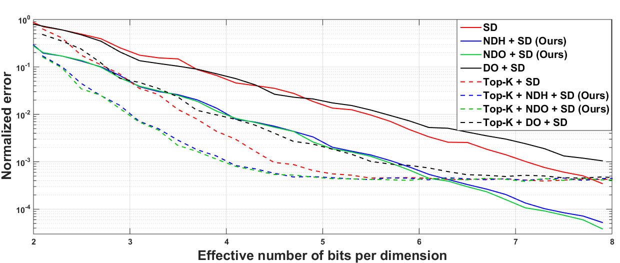


Fig. 1(b) compares the empirical convergence rate, defined as versus the bit-budget constraint, i.e., bits per dimension, for solving the least squares problem , where , and the entries of are drawn from Gaussian-cubed as before. If the algorithm does not converge, the empirical rate is clipped at . Unquantized GD has a constant rate equal to [31]. DQGD proposed in [6] used a predefined sequence of dynamic ranges, and nearest-neighbor scalar quantization. In comparison, we normalize the input to the quantizer by norm, and since it is a scalar quantity, we assume that it is transmitted with infinite precision. A more comprehensive justification for sending scalars can be found in App. F. We observe that Near-Democratic Embeddings (NDE) perform at par with Democratic Embeddings (DE), and both ensure convergence at very low bit-budgets. Sometimes, it may even perform better because NDE allows us to choose , and hence as seen before, no resolution is lost due to the fixed bit-budget. Moreover, the computational advantage of NDE is evident from Fig. 1(c) where we plot the wall-clock time (in seconds) (averaged over 10 realizations) vs. dimension to find these embeddings. The DE’s are obtained by solving (5) using CVX and the NDE’s are obtained from the closed form expression . Here, for each , the value of is chosen to be . This plot was obtained on a Dell Vostro with an Intel i5 1.60GHz processor running MATLAB R2014b. Finally, in Fig. 1(d), we solve the -regularized least squares problem for the MNIST dataset [34]. We use gradient descent where the gradients are compressed, first by random sparsification followed by an aggressive -bit quantization for the retained coordinates, so that effectively bits are used per dimension. We note that NDE’s using random orthonormal frames converge for , whereas the vanilla compression scheme fails. For least-square simulations, we use the step-size given by Thm. 2.


For general convex & non-smooth objectives, we train a support vector machine where the subgradients are quantized using -bits per dimension. Each worker has datapoints for . We want to solve the following optimization problem in which our aim is to minimize the hinge loss: . We compare the performance of our proposed DQ-PSGD algorithm with naive scalar quantization as well as unquantized projected stochastic subgradient descent. The stochasticity in the subgradient oracle evaluation arises from randomly subsampling the dataset to compute the subgradient at every iteration. We consider the number of datapoints , and dimension of the problem . For Figs. 2(a) and 2(b), the data corresponding to each class is generated independently from Gaussian distributions with different means. We consider random orthonormal frames for computing NDE’s. Fig 2(a) plots the suboptimality gap (averaged over different realizations) versus the number of iterations. The optimal value for computing the suboptimality gap in Fig. 2(a) is obtained by using the interior point solver provided by CVX [33]. We effectively have , i.e., less than one bit per dimension. In other words, since we only have a total of bits available, the subgradient is randomly sparsified by making certain coordinates zero, and the remaining vector is quantized using -bit per dimension. There is a significant difference in performance when randomly sparsifying of the coordinates with and without NDE’s. We also consider top-K sparsification [18] with and without NDE’s. We choose , i.e., we decide to retain only the top of the coordinates. When we employ both sparsification and quantization techniques simultaneously to compress the gradient but only have a fixed total number of bits available, there arises a tradeoff between how many coordinates we want to retain and the number of bits allotted for quantizing each retained coordinate. Smaller means more bits per coordinate i.e., better resolution for scalar quantization of the retained coordinates, and vice versa. In random sparsification, we retain coordinates with -bit allotted for each. For top-K, we retain coordinates and allot bits for quantizing each of them. Although top-K is expected to perform better than random sparsification, choosing the value of heuristically may yield poorer performance (despite the additional computation required for determining the top K coordinates) as in this case. We also plot the classification error, that is the percentage of misclassified samples in the training set at every iteration in Fig. 2(b) and observe a similar trend for the different sparsification and quantization schemes.
Figs. 2(c) and 2(d) consider the MNIST dataset [34], and the problem of training an SVM to distinguish the digit from digit . Fig. 2(c) shows how the objective function value decreases with the number of iterations. Fig. 2(d) plots the classification error on the hold-out test set for each iteration. We consider only realization for this setting and let . For top-K, we retain the top coordinates, while ensuring that the total bit-budget remains same for all the schemes, i.e., a total of bits. For random sparsification with and without NDE’s, coordinates are chosen randomly from the gradient which and bit is allotted to each of them. For top-, we now choose to retain the top coordinates of maximum magnitude, allot bit to quantize each of them, and make the rest zero. Since the number of retained coordinates is the same for both random and top-K sparsification in this setting i.e., , top-K performs better as expected. For this set of simulations, we have chosen a nominal step-size empirically, and kept it constant for a fair comparison of different algorithms.


Multi-worker simulations. We consider two problems. Fig. 3(a) considers a regression model that solves: . Here, denotes the local dataset at node , for . The dimension of the problem is , workers with each worker having local datapoints. The dataset is generated synthetically from a model according to the noisy planted model , where is the regression output and the rows of , i.e. are the data vectors. We let and the entries of the data matrix .
Although our theoretical analysis is for convex functions, we also provide simulations for non-convex settings. In Fig. 3(b), we train a convolutional neural network (CNN) over workers to do multi-class classification on the CIFAR-10 [35] image classification dataset that contains training and test images from classes. The entire dataset is distributed across these workers in a non-i.i.d. fashion, so that each worker has images from at most out of the classes. As can be seen from the plot, with a bit-budget of bits per dimension per worker, our proposed near-democratic source coding (NDSC) scheme with randomized Hadamard frame outperforms naïve quantization with the same bit-budget () which fails to even converge. As a matter of fact, naïve quantization requires a higher budget of bits per dimension per worker to achieve a performance comparable to that of NDSC. Further detailed simulations are provided in Appendix I.
6 Conclusions
In this work, we show that democratic embeddings can yield minimax optimal distributed optimization algorithms under communication constraints when employed in source coding schemes. For smooth & strongly convex objectives, we propose DGD-DEF, which employs error feedback to achieve linear convergence. For the case of general convex & non-smooth objectives, when the output of the stochastic subgradient oracle is quantized using a democratic source coding scheme, DQ-PSGD attains minimax optimal convergence rate. We note that although DSC theoretically attains minimax optimal performance to within constant factors, computing democratic embeddings can be computation and memory intensive. We also propose a randomized Hadamard construction for fast near-democratic embeddings. Finally, we extend the analysis and simulate our algorithms for multi-worker setups. A potential limitation of the proposed optimization approaches is that the curvature information is not utilized, which we leave as future work.
References
- [1] R. Bekkerman, M. Bilenko, and J. Langford, Scaling up Machine Learning: Parallel and Distributed Approaches. USA: Cambridge University Press, 2011.
- [2] P. Kairouz and et. al., “Advances and open problems in federated learning,” Foundations and Trends® in Machine Learning, vol. 14, no. 1–2, pp. 1–210, 2021.
- [3] M. Li, D. G. Andersen, J. W. Park, A. J. Smola, A. Ahmed, V. Josifovski, J. Long, E. J. Shekita, and B.-Y. Su, “Scaling distributed machine learning with the parameter server,” in Proceedings of the 11th USENIX Conference on Operating Systems Design and Implementation, 2014, p. 583–598.
- [4] M. M. Amiri and D. Gündüz, “Machine learning at the wireless edge: Distributed stochastic gradient descent over-the-air,” IEEE Transactions on Signal Processing, vol. 68, pp. 2155–2169, 2020.
- [5] R. Saha, S. Rini, M. Rao, and A. J. Goldsmith, “Decentralized optimization over noisy, rate-constrained networks: Achieving consensus by communicating differences,” IEEE Journal on Selected Areas in Communications, vol. 40, no. 2, pp. 449–467, 2022.
- [6] C.-Y. Lin, V. Kostina, and B. Hassibi, “Differentially quantized gradient descent,” in 2021 IEEE International Symposium on Information Theory (ISIT), 2021, pp. 1200–1205.
- [7] P. Mayekar and H. Tyagi, “RATQ: A universal fixed-length quantizer for stochastic optimization,” in Proceedings of the Twenty Third International Conference on Artificial Intelligence and Statistics, 2020, pp. 1399–1409.
- [8] D. Alistarh, D. Grubic, J. Li, R. Tomioka, and M. Vojnovic, “QSGD: Communication-efficient SGD via gradient quantization and encoding,” in Advances in Neural Information Processing Systems, vol. 30. Curran Associates, Inc., 2017, pp. 1709–1720.
- [9] C. A. Rogers, “Covering a sphere with spheres,” Mathematika, vol. 10, p. 157–164, 1963.
- [10] Y. Lyubarskii and R. Vershynin, “Uncertainty principles and vector quantization,” IEEE Trans. Inf. Theor., vol. 56, no. 7, p. 3491–3501, 2010.
- [11] A. T. Suresh, F. X. Yu, S. Kumar, and H. B. McMahan, “Distributed mean estimation with limited communication,” in Proceedings of the 34th International Conference on Machine Learning, 2017, pp. 3329–3337.
- [12] A. Abdi and F. Fekri, “Quantized compressive sampling of stochastic gradients for efficient communication in distributed deep learning,” in Proceedings of the AAAI Conference on Artificial Intelligence, vol. 34(04), 2020, pp. 3105–3112.
- [13] R. Hadad and U. Erez, “Dithered quantization via orthogonal transformations,” IEEE Transactions on Signal Processing, vol. 64, no. 22, pp. 5887–5900, 2016.
- [14] J. Bernstein, Y.-X. Wang, K. Azizzadenesheli, and A. Anandkumar, “signSGD: Compressed optimisation for non-convex problems,” in Proceedings of the 35th International Conference on Machine Learning, 2018, pp. 559–568.
- [15] S. P. Karimireddy, Q. Rebjock, S. Stich, and M. Jaggi, “Error feedback fixes SignSGD and other gradient compression schemes,” in Proceedings of the 36th International Conference on Machine Learning, 2019, pp. 3252–3261.
- [16] W. Wen, C. Xu, F. Yan, C. Wu, Y. Wang, Y. Chen, and H. Li, “Terngrad: Ternary gradients to reduce communication in distributed deep learning,” in Advances in Neural Information Processing Systems, vol. 30. Curran Associates, Inc., 2017, pp. 1509–1519.
- [17] V. Gandikota, D. Kane, R. Kumar Maity, and A. Mazumdar, “vqSGD: Vector quantized stochastic gradient descent,” in Proceedings of The 24th International Conference on Artificial Intelligence and Statistics, 2021, pp. 2197–2205.
- [18] S. U. Stich, J.-B. Cordonnier, and M. Jaggi, “Sparsified SGD with memory,” in Proceedings of the 32nd International Conference on Neural Information Processing Systems, ser. NIPS’18. Curran Associates Inc., 2018, p. 4452–4463.
- [19] J. Wangni, J. Wang, J. Liu, and T. Zhang, “Gradient sparsification for communication-efficient distributed optimization,” in Advances in Neural Information Processing Systems. Curran Associates, Inc., 2018.
- [20] P. Mayekar and H. Tyagi, “Limits on gradient compression for stochastic optimization,” in 2020 IEEE International Symposium on Information Theory (ISIT), 2020, pp. 2658–2663.
- [21] B. S. Kashin, “Diameters of some finite -dimensional sets and classes of smooth functions,” Mathematics of the USSR-Izvestiya, vol. 11, no. 2, pp. 317–333, apr 1977.
- [22] E. J. Candes and T. Tao, “Decoding by linear programming,” IEEE Transactions on Information Theory, vol. 51, no. 12, pp. 4203–4215, 2005.
- [23] W.-N. Chen, P. Kairouz, and A. Ozgur, “Breaking the communication-privacy-accuracy trilemma,” in Neural Information Processing Systems (NeurIPS), 2020.
- [24] S. Caldas, J. Konečny, H. B. McMahan, and A. Talwalkar, “Expanding the reach of federated learning by reducing client resource requirements,” 2018. [Online]. Available: https://arxiv.org/abs/1812.07210
- [25] M. Safaryan, E. Shulgin, and P. Richtá rik, “Uncertainty principle for communication compression in distributed and federated learning and the search for an optimal compressor,” Information and Inference: A Journal of the IMA, 2021.
- [26] R. Saha, M. Pilanci, and A. J. Goldsmith, “Minimax optimal quantization of linear models: Information-theoretic limits and efficient algorithms,” 2022. [Online]. Available: https://arxiv.org/abs/2202.11277
- [27] C. Studer, T. Goldstein, W. Yin, and R. G. Baraniuk, “Democratic representations,” 2014. [Online]. Available: https://arxiv.org/abs/1401.3420
- [28] I. Dumer, “Covering spheres with spheres,” Discrete & Computational Geometry, vol. 38, pp. 665–679, 2016.
- [29] A. Gersho and R. M. Gray, Vector Quantization and Signal Compression. Springer International, 1992.
- [30] A. D. Wyner, “Random packings and coverings of the unit n-sphere,” The Bell System Technical Journal, vol. 46, no. 9, pp. 2111–2118, 1967.
- [31] Y. Nesterov, Introductory Lectures on Convex Optimization: A Basic Course, 1st ed. Springer Publishing Company, Incorporated, 2014.
- [32] D. Alistarh, T. Hoefler, M. Johansson, N. Konstantinov, S. Khirirat, and C. Renggli, “The convergence of sparsified gradient methods,” in Advances in Neural Information Processing Systems, vol. 31. Curran Associates, Inc., 2018.
- [33] M. Grant and S. Boyd, “CVX: Matlab software for disciplined convex programming, version 2.1,” http://cvxr.com/cvx, Mar. 2014.
- [34] Y. LeCun, L. Bottou, Y. Bengio, and P. Haffner, “Gradient-based learning applied to document recognition,” http://yann.lecun.com/exdb/mnist/, pp. 2278–2324, 1998.
- [35] A. Krizhevsky, V. Nair, and G. Hinton, “Cifar-10 (canadian institute for advanced research).” [Online]. Available: http://www.cs.toronto.edu/~kriz/cifar.html
- [36] L. Bottou, F. E. Curtis, and J. Nocedal, “Optimization methods for large-scale machine learning,” 2016. [Online]. Available: https://arxiv.org/abs/1606.04838
- [37] I. Haviv and O. Regev, The Restricted Isometry Property of Subsampled Fourier Matrices, pp. 288–297. [Online]. Available: https://epubs.siam.org/doi/abs/10.1137/1.9781611974331.ch22
- [38] O. Christensen, An Introduction to Frames and Riesz Bases, ser. Applied and Numerical Harmonic Analysis. Springer International Publishing, Birkhäuser, Cham, 2016. [Online]. Available: https://doi.org/10.1007/978-3-319-25613-9
Appendices
Appendix A Proof of Lemma 2: Near-Democratic Embeddings with Random Orthonormal Frames
Let and denote the columns of and respectively, where , are defined in §2.1. For , since , we have,
For any , let . Then,
where . Note that is uniformly random on the unit sphere in , i.e., has identical distribution as where . Due to rotational invariance of Gaussian distribution, for any fixed such that , has identical distribution as , where is the first canonical basis vector. From concentration of measure for uniform distribution on the unit sphere,
Using a union bound,
Setting yields,
which completes the proof.
Appendix B Proof of Lemma 3: Near-Democratic Embeddings with Randomized Hadamard Frames
Denote , and let . Here, is of the form , with each chosen i.i.d. For any and , a Chernoff-type argument gives,
Now,
where the last inequality follows from a bound on hyperbolic cosine. This gives us . Setting gives the tightest bound,
Similarly, one can show that,
Since , union bound gives,
Setting yields,
Since , this completes the proof.
Appendix C Proof of Thm. 1: Quantization Error: (N)-DSC
Let denote either or . Then, given an input to , let be the (near) democratic representation, be the normalized input to , be the encoder output, and be the decoder output. The error incurred after encoding and subsequent decoding is
The last inequality follows since,
Since is a Parseval frame, and non-zero eigenvalues of are the same as those of , we have . To upper bound the quantization error , note that if we originally had a total budget of -bits, the number of bits per dimension to uniformly quantize is now , i.e., quantization points per dimension. From (11),
So, if we use from Lemma 1,
Similarly, for , using Lemma 3,
This completes the proof.
Appendix D Proof of Thm. 2: Convergence Rate of DGD-DEF
For an -bit Quantized Gradient Descent (QGD) algorithm (defined in §4 and [6, Def. IV.1]), the minimax convergence rate (2) over the function class is lower bounded as , where . The convergence analysis makes use of a recursive invariant satisfied by the trajectory of DGD-DEF. Consider the two descent trajectories: DGD-DEF and unquantized GD with the same step size , starting at the same location . Then using triangle inequality, at each iteration we have,
where . From algorithm pseudocode 1, note that , i.e., DGD-DEF computes the gradient at the unquantized trajectory . Decay of the first term is given by the convergence guarantee of unquantized GD [31], which states that , where is the convergence rate for unquantized GD with step size . An upper bound to the second term is obtained from our quantization scheme, as per the following auxiliary lemma.
Lemma 5.
For , at any iteration , the quantizer input satisfies , where the sequence is given by . Here if democratic embeddings are used, and if near-democratic embeddings are used.
Proof.
This is proved using induction. For , we have . Since , recalling that and is -smooth, we have,
and so the lemma holds true for . From triangle inequality,
The first term can be upper bounded as,
Furthermore, from Thm. 1,
where depends on whether we choose democratic or near-democratic embeddings for our source coding scheme, and the second inequality is the induction hypothesis. Using these, we can upper bound the magnitude of the quantizer input as,
This completes the proof. ∎
The proof of Thm. 2 is similar to the [6, Thm. III.1] except for appropriate modifications due to our proposed source coding schemes: DSC and NDSC. Since for ,
the first term can be upper bounded from the descent guarantee of unquantized GD trajectory as,
The second term can be upper bounded as
where the inequalities follow from the definition of and Lemma 5. So we have, . There are now three possibilities:
- 1.
: The geometric sum is computed as,
- 2.
: In this case,
- 3.
: The case parallels the first case by interchanging the role of and , and we get,
the proof is complete by concisely expressing the above three cases as:
| (18) |
Appendix E Proof of Thm. 3: Convergence Rate of DQ-PSGD
Consider the optimization problem: , where, is a convex set, and is convex, but not necessarily smooth. satisfies for some known . We assume oracle access to noisy subgradients of . The oracle output for any input query point to be unbiased, i.e., , where, denotes the subdifferential of at the point , and uniformly bounded, i.e., for all , for some . An -bit quantizer is defined to be a (possibly randomized) pair of mappings , with the encoder mapping and the decoder mapping . Let denote the set of all such -bit quantizers. For any pair of objective function and oracle , and an -bit quantizer , let denote the composition oracle that outputs for each query . Let be an optimization protocol as defined in §1. We consider the minimax expected suboptimality gap (4). The convergence rate of DQ-PSGD depends on the quantizer design of .
The performance of any quantizer is determined by the following two quantities: The worst-case second moment, i.e.,
and the worst-case bias, i.e.,
For any such quantizer , from [7, Thm. 2.4], the worst-case expected suboptimality gap of quantized projected subgradient algorithm after iterations, with step-size is,
| (19) |
We design so that for any input , encodes the magnitude (gain) of the input and the direction (shape) of separately, and forms the estimate of by multiplying the estimates for the magnitude and direction. In other words,
where , and .
It is assumed that given , and are independent of each other. From [7, Thm. 4.2], if is unbiased, i.e., for all satisfying , then,
The uniformly dithered quantizer for is described next. Let the dynamic range of be the known uniform upper bound, . Consider quantization points uniformly spaced along the interval and let and . For any input , the output of the gain quantizer is defined to be:
| (20) |
where, . If a fixed number of bits (typically ) are used, it can be easily shown that is unbiased. For designing , we consider two separate cases: The high-budget regime () and the sub-linear budget regime (). The proof Thm. 3 is completed after combining the results of §E.1 and §E.2.
E.1 High-budget regime
Let the input to be such that . For , if denotes the democratic embedding of with respect to , then . Let the coordinate-wise uniformly dithered quantizer () be as in [7], in which we do dithered quantization (20) of each coordinate of independently, using bits per dimension and a dynamic range of . The output is . Since is unbiased, the output of is also unbiased, i.e., . Since both and are conditionally independent of each other, the bias of , i.e., the worst-case bias . To evaluate the worst-case second moment of , from [7, Thm. 4.2], . Since the dynamic range of is , the worst-case bias . For and any such that , we have . The final inequality follows since . Moreover, since the dynamic range for is , we have for all . So, the worst-case second moment is . Substituting these values for and in (19), we get the result. A similar result with a dependence on dimension can be proved for NDSC.
E.2 Sub-Linear budget regime
When , the total bit-budget is , i.e., we have less than -bit per coordinate. For brevity, let . The statements here can be easily generalized to the case of . To allocate bits to each coordinate of a vector in so that on an average -bits per dimension is utilized, we choose coordinates uniformly at random; allocate -bit to each of these coordinates, and allocate -bit to the remaining coordinates. This essentially subsamples the vector in to a smaller dimensional vector in , and subsequently doing a -bit quantization of the vector in , while decoding the other coordinates as . Since and we are subsampling and want to be unbiased, we need to scale the quantized output by a factor of . So, the democratic representation + subsampling + -bit quantization scheme as is . Here, is the canonical basis vector, with denotes the random indices chosen in the subsampling step, and denotes the indicator function, since the coordinates not selected in the subsampling step are decoded as . Unbiasedness ensures that . Moreover,
The last equality follows as sampling coordinates uniformly at random from coordinates implies . Since , the worst-case second moment is . Substituting these values of and in (19), the convergence rate when is . This completes the proof.
Appendix F Quantizing the norm
For simplicity, the statement of Thm. 2 assumes that the norm of the input to the quantizer can be transmitted perfectly without lossy quantization. If we use a constant number of bits (typically, bits depending on the machine precision) to uniformly quantize , the total number of bits required to quantize the vector is bits per dimension as . Hence, the bit-budget is respected asymptotically and the additional constant number of bits is negligible for high dimensional problems. To take account the error due to quantizing , note that if ,
The last inequality follows from triangle inequality. Since we employ DSC for the shape quantizer, the first term can be upper bounded using Thm. 1. The second term can be upper bounded as,
which is an additional constant error. The whole convergence analysis follows through with this constant additive error too.
Appendix G Closed Form for Near-Democratic Embeddings (NDE)
For any , its NDE, with respect to a frame (for ) is defined to be the solution of the minimization problem . Its Lagrangian is,
. This gives,
So, and,
The last equality follows from the fact that we choose our frames to be Parseval, i.e., they satisfy . Random Haar orthonormal or Random Hadamard frames are Parseval frames and hence NDEs can be computed very efficiently.
Appendix H Extension to General Compression Schemes
For any general (possibly stochastic) lossy compression scheme like sparsification, standard dithering, etc, instead of compressing the input directly, compressing its (near) democratic embedding , will consistently improve robustness by ensuring that the error due to compression has independent/weak-logarithmic dependence on dimension .
Theorem 4.
For any unbiased compression operator that satisfies for all , DSC/NDSC with corresponding encoding and decoding functions defined for any as and , satisfies , where if , and if .
Proof.
For a given frame , from linearity of expectations, . Here, can represent either the DE () or the NDE (). The approximation error can be bounded uniformly (without the expectation) as,
| (21) |
follows since . If , then from Lemma , . Substituting this in (21), we get the result for DE with . Similarly, if , using Lemma , . Substituting this once again in (21), we get the result for NDE with . This completes the proof. ∎
Appendix I Extension to multiple workers

To extend our algorithm to a setup with multiple workers, consider the following optimization problem over workers and a parameter-server (PS):
| (22) |
As shown in Fig. 4, the objective is the sum of multiple , each known privately to a corresponding node . Node can compute the gradient (or a subgradient, ) for any , and communicate it to the PS. For general convex, non-smooth functions with stochastic subgradient oracle, Alg. can be extended to multiple workers by incorporating an additional consensus step at the PS. The pseudocode is provided below in Alg. 3.
Convergence analysis of SGD (from any standard text such as [36]) tells us that the upper bound on the expected suboptimality gap scales proportionally with the variance of the stochastic subgradient, i.e. , where , for all and . Succinctly stated, similar to Thm. of the main paper, we have,
Let be the global stochastic subgradient at the PS if there were no quantization constraints. Young’s inequality states that for any and any , we have . Using this with , in the presence of quantization, the variance can be upper bounded as,
Here, the equality follows from the fact that we assume the gradient quantization and the stochastic subgradient oracle at each node to be independent of each other (so that the cross-terms vanish). Also, is a known upper bound on the inherent stochasticity of the subgradient oracle, i.e. for all . is the additional variance introduced due to quantization at each node, and it depends on the source coding scheme we use at each node. We next consider expressions for for the naïve and our proposed quantization strategies.
Consider the stochastic uniform quantizer as defined below. This is similar to the quantizer defined in App. E of the main paper (with slight differences in scaling that can be easily accounted for with a more detailed analysis). For an input , let denote the value of its coordinate. The stochastic uniform quantizer quantizes each coordinate of independently, i.e. the quantizer output is given by , where the scalar quantizer is defined next. Along each dimension, consider the quantization points , given by,
For any coordinate , , suppose for some . Then the output of is,
Note that this quantizer satisfies for any , and its variance can be upper bounded as,
As can be seen from above, for the naïve stochastic uniform quantizer with an input that satisfies , this gives us a worst-case upper bound on the quantization variance as:
since gives the worst-case input . With an application of Jensen’s inequality, this gives us a convergence rate of DQ-PSGD that scales as follows:
| (23) |
We ignore the dependence on in the above expression since it does not depend on the quantizer design. The dependence of this convergence rate on the dimension can be detrimental for high dimensional problems. We show that using our proposed source coding schemes, we can get rid of this linear dependence on .
Our proposed algorithm DSC, first computes the democratic embedding, quantizes it the embedding using a stochastic uniform quantizer in the encoding process, and finally computes the inverse embedding while decoding. Democratic embeddings have the property that for some constant with high probability. Substituting this -norm in the expression of the quantizer variance yields,
This gives us a dimension-independent bound on the quantizer variance, and consequently on the convergence rate, which now scales as,
| (24) |
Similarly, if we use near-democratic embeddings (using a random orthonormal or a randomized Hadamard frame), we have, with high probability, , which yields an upper bound on the convergence rate of DQ-PSGD as,
| (25) |
giving us a mild logarithmic scaling instead of a (worse) scaling as in the naïve case. In what follows, we do some additional simulations for training models over multiple workers. We consider a setup of multi-worker linear regression, wherein our goal is the solve the optimization problem:
| (26) |
Here, denotes the local dataset at node , for . The dimension of the problem is , workers with each worker having local datapoints. The learning rate of SGD is taken to be a constant . The dataset is generated synthetically from a model according to the planted model , where is the regression output and the rows of , i.e. are the data vectors. In Fig. 5, the entries of and are generated by first drawing i.i.d. samples from and raising them to the third power, i.e. . All plots are averaged over independent trials and the synthetic data is also generated independently each time. The two figures depict plots for two different values of and bits per dimension per user. We also simulate for another heavy-tailed distribution of and the entries of the data matrix in Fig. 6.


In addition to this, it is also possible to consider an extension of DGD-DEF to optimizing smooth and strongly convex objective functions over multiple workers and obtain faster convergence rates, by considering the extension in [6, Sec. 5] in which each worker does error feedback independently. However, a complete characterization and extension of the idea of error feedback to multiple workers (in which the error feedback term compensates for errors from all workers) is still an open problem (as noted in [6, Sec. V-C]) and is beyond the current scope of our work.
We also train a simple neural network in the Federated Learning setup to do multi-class classification on the CIFAR-10 [35] image classification dataset that contains training and test images from classes. We consider workers and the entire dataset is distributed across these workers in a non-i.i.d. fashion, so that each worker has images from at most out of the classes.
Each worker locally trains a simple CNN model described next. The CNN has a Convolution Batch Normalization layer, followed by a max pooling layer, followed by another Convolution Batch Normalization layer. This is followed by three fully-connected layers. We use SGD with global momentum at the parameter server to the train the model. The learning rate is taken to be , and the momentum parameter as . A coefficient of is considered for -regularization (or weight-decay regularization) to prevent overfitting. The batch-size is taken to be . All simulations were carried out on NVIDIA GeForce GTX Ti with a CUDA Version .
The neural network simulation results are presented in Fig. 7. Here, we plot the test-accuracy versus the number of communication rounds between the workers and the PS. As can be seen from the plot, with a bit-budget of bits per dimension per worker, our proposed near-democratic source coding (NDSC) scheme with randomized Hadamard frame outperforms naïve quantization with the same bit-budget () which fails to even converge. As a matter of fact, naïve quantization requires a higher-budget of bits per dimension per worker to achieve a performance comparable to that of near-democratic source coding (NDSC).
Appendix J Comparison of Different Classes of Randomized Frames for Computing Democratic Embeddings
The Uncertainty Principle (UP) for random matrices (Definition in the main paper), is closely related to the Restricted Isometry Property (RIP) for random matrices introduced in [22].
Definition 3.
(Restricted Isometry Property (RIP)) A matrix is said to satisfy the Restricted Isometry Property of order with constant , if for every -sparse vector (i.e. a vector with at most non-zeros entries), the following holds true:
| (27) |
Comparing Definition 3 above with the definition of UP (Definition in the main paper), it can be seen that any matrix that satisfies RIP with parameters , satisfies UP with parameters . In other words, randomly constructed frames which satisfy the UP with high probability, are strongly related to sensing matrices with small restricted isometry constants. Since the upper Kashin constant is given by , in order to achieve embeddings having small norm, one is therefore interested in finding frames satisfying the UP with small and large .
J.1 Sub-Gaussian Random Matrices
Definition 4.
(Sub-Gaussian random variable) A random variable is called sub-Gaussian with parameter if
| (28) |
From [10], we have the following result regarding the uncertainty principle parameters of random sub-Gaussian matrices:
Theorem 5.
[10, Theorem 5]: (Uncertainty principle for sub-Gaussian matrices) Let the entries of be i.i.d. zero-mean sub-Gaussian random variables with parameter . Let for some . Then with probability at least , the random matrix satisfies the UP with parameters:
| (29) |
where, are absolute constants.
Note: Random sub-Gaussian matrices are NOT tight frames. However, [10, Lemma 4.8] and [10, Corollary 4.9] show that (as constructed above) is an approximate Parseval frame with high probability, i.e. has frame bounds and for some small . Substituting in the values to obtain the upper Kashin constant, we have,
| (30) |
Note that the upper Kashin constant has a logarithmic dependence on the aspect ratio of the frame, . Since is essentially treated as a constant, is a constant. However, the -bit floating point entries of a sub-Gaussian matrix need to be stored in the memory and furthermore, multiplying the dense matrix by a vector can take up to a worst case of time. Hence, choosing sub-Gaussian frames can be intensively computation as well as memory demanding.
J.2 Random Orthonormal Matrices
Random orthonormal matrices refer to matrices whose rows are orthonormal. Such matrices can be obtained by randomly selecting the first rows of a randomly generated orthonormal matrix. We state a result from [10]. If denotes the space of all orthogonal matrices with the normalized Haar measure, then , where is the orthogonal projection on the first coordinates, denotes the space of all orthonormal matrices. The probability measure on is induced by the Haar measure on .
Theorem 6.
[10, Theorem 4.1]: (UP for Random Orthonormal Matrices) Let and . Then with probability at least , a random orthonormal matrix satisfies the uncertainty principle with parameters
| (31) |
where is an absolute constant.
Note that random orthonormal matrices are Parseval frames, i.e. . So, the upper Kashin bound is given by:
| (32) |
This once again shows that is a constant.
J.3 Random Matrices with Fast Transforms
Matrices with fast transforms refer to structured matrices like Fourier transform matrix, etc. for which fast algorithms exist to compute the forward transform efficiently. To analyze the RIP properties of our proposed randomized Hadamard matrix construction, , we recall the following theorem from [37].
Theorem 7.
[37, Theorem 4.5] For sufficiently large and , a unitary matrix with entries of absolute value , and for sufficiently small , the following holds: For some , let be a matrix whose rows are chosen uniformly at random and independently from the rows of , multiplied by . Then, with probability , the matrix satisfies the restricted isometry property of order with constant .
The upper Kashin constant for such a matrix can be computed approximately as follows:
| (33) |
Furthermore, since the definition of UP requires , it is apparent that if we scale the entries of the matrix by a constant factor, the parameter of UP also scales by the same factor. So, in Thm. 7, if we multiply the matrix by to negate the effect of multiplying by as in the statement of the theorem in order to get , then the corresponding UP parameters of are:
| (34) |
where is dictated by (33).
| (35) |
We see that our proposed randomized Hadamard construction , which provides computational and memory savings, as seen in the main paper falls in this class of random matrices with fast transforms. However, for such matrices, since is not a constant and scales as , when is large, computing democratic embedding does not yield much benefit as compared to the near-democratic embedding. From Lemma of the main paper, the -norm of the near-democratic embedding of also scales as .
In other words, for random matrices with fast transforms, asympotically (i.e. for large ), near-democratic embeddings have -norm as good as democratic embeddings. However, unlike sub-Gaussian and random orthonormal frames, since the entries of are , only the signs need to be stored (which amounts to -bit per entry, hence saving memory requirements), and can effectively be obtained in additions, which is much less computationally demanding.
Appendix K Proof of Lemma : Covering efficiency: DSC & NDSC
Suppose the input to the encoders satisfy . From Thm. , . Since an -bit quantizer has a range of finite cardinality , using eq. , we have . Similarly, the expression for follows.
Appendix L Additional Discussions and Remarks
L.1 Discussions on Other Related Works
A succinct comparison of DSC and NDSC with some of the existing quantization/sparsification schemes is provided in Table I.
We characterize each compression scheme by its bit requirement and the normalized error.
For any input vector with , let the output of a compression scheme be denoted as .
Then the normalized error is defined to be .
Sign Quantization [14, 15]. Sign quantization strategies quantize each coordinate of the quantizer input to either or depending on its sign.
With proper magnitude scaling, they are effective in quantizing using only -bit per dimension.
To get an expression for the normalized error, if we additionally assume that each coordinate of is bounded, i.e. , then the error incurred can be upper bounded as , where is the dimension of .
A similar situation arises with QSGD when more than -bit are used to quantize each coordinate of .
The situation is similar for TernGrad [16], that uses three numerical levels to quantize the gradients for distributed training of neural networks.
QSGD [8]. QSGD uses quantization levels for each coordinate.
If we were to use -bits per dimension, then we have .
[8, Thm. 3.2] specifies the bit requirement and normalized error.
This result provides an upper bound on the expected bit requirement, since it is a Variable-length code.
Our work considers fixed-length quantizers wherein the bit-budget per dimension () is pre-specified as a constraint.
Moreover, we study optimality of fixed-length quantization schemes for all values of .
In contrast to this, QSGD only considers .
Furthermore, for worst-case inputs , the performance of QSGD is far from optimal, whereas our quantizers are designed to guarantee minimax optimal performance.
Vector Quantized SGD [17]. vqSGD constructs a convex hull using a finite number of points and quantize their vector to one of the points randomly.
They also consider both communication and privacy parameters of their coding scheme simultaneously.
From [17, Table 2], the error of vqSGD scales as with the dimension , as compared to and for DSC/NDSC respectively.
Here, is a constant.
Top- sparsification [18] is a common gradient sparsification technique.
Here, denotes the number of retained coordinates.
The bit-requirement arises from the need to communicate the values of the chosen coordinates, and the comes from the number of the ways out of indices can be chosen, which also needs to be conveyed.
This source coding scheme requires a computation of due to the fact that the coordinates must be sorted in order to be able to choose the top out of them.
Random sparsification [19] is another simple strategy which randomly chooses the out of indices.
Gradient sparsification and quantization are complementary to each other in reducing the communication requirements.
We show DE/NDE can be used in conjunction with existing gradient sparsification and quantization techniques to further improve the performance of the latter.
SimQ+ [20]. SimQ+ addresses the problem of designing quantizers for optimization over general -spaces.
SimQ+ relies on a more fundamental quantizer, SimQ that exploits the fact that any point inside the unit ball of can be represented as a convex combination of at most points.
SimQ then samples one of these points.
In this sense, it is similar to vqSGD.
For Euclidean spaces, i.e. (considered in our work), [20, Thm. 3.1] shows that SimQ+ uses bits to achieve the optimal suboptimality gap scaling of for general convex and non-smooth functions.
The computational complexity of SimQ+ is .
This is because SimQ+ requires repetitions of SimQ.
SimQ involves sampling from an -dimensional probability distribution [20, Alg. 2].
Efficient methods for sampling from high-dimensional distributions (like Walker Alias method) entails complexity.
Moreover for -spaces, SimQ+ requires repetitions of SimQ.
This results in a total complexity of .
Consequently, for , the performance of our proposed quantizers is the same as SimQ+.
However, for any other value of , SimQ+ is no longer optimal as noted in [20, §7].
In order to make SimQ+ operate under any arbitrary precision constraint , requires us to modify it by incorporating heuristics like uniform sampling without replacement.
But doing so causes the SimQ+ quantizer design to lose optimality with undesirable logarithmic factors appearing between upper and lower bounds.
Although the gap is practically insignificant, our quantizer design using democratic embeddings resolves this open question for spaces.
This is especially true in the sublinear bit-budget regime, when .
RATQ [7]. The Rotated Adaptive Tetra-iterated Quantizer (RATQ) involves Hadamard transforms and appropriately chosen quantizer dynamic ranges to achieve a performance which is factor close to optimal for stochastic optimization, with a computational complexity of . They consider the optimization of general convex and non-smooth objective functions with access with a stochastic subgradient oracle, which corresponds to Thm. of our work. Compared to this, our proposed scheme DSC (with random orthonormal frame) achieves a performance to within a constant factor of optimality with a complexity of , and NDSC achieves a performance factor away from optimality while entailing a complexity. Hence from a high-level perspective, RATQ has a performance somewhere in between DSC and NDSC for stochastic optimization. Note that since RATQ makes use of standard dithering [7, Alg. 5], it is an inherently stochastic quantizer. Consequently, it is not straightforward to see how RATQ could be applied to settings which require deterministic quantizers such as the optimization of smooth, strongly-convex objective functions in our work. For analyzing deterministic settings, we require a uniform upper bound on (i.e. without any expectation) for any quantizer and input . DSC and NDSC can be designed for deterministic quantizers as well (cf. Eq. ), which does nearest-neighbor quantization.
Appendix M A note on randomized frame constructions
The definition of a frame as given in Def. of the main paper is quite general [38]. A frame is the same as a wide matrix with full row rank, i.e. . More specifically, a full rank matrix with singular values satisfies
for any . That is, and are the upper and lower frame bounds respectively. The concept of frames is a very widely used concept in linear algebra and not specific to our work. For an inner-product space, a frame is a set of (possibly) linearly-dependent vectors that act as a generalization of a basis. Because it consists of linearly dependent vectors, the representation of any vector in terms of a frame is not unique. Consequently, frames provide a robust way of representing a vector due to this redundancy.
Although frames are abundant, what is more interesting to our work are frames that satisfy the uncertainty principle as in Def. in the main paper. Our randomized frame constructions satisfy the uncertainty principle for appropriate values of parameters such that the upper Kashin constant (as defined in Lemma ) is a small constant.
In what follows, we show a full rank matrix that satisfies all the properties of a frame, but does not satisfy uncertainty principle with desirable values of the parameters . As a consequence, the upper Kashin constant is not small and the inequality is Lemma is vacuous. Consider the matrix:
i.e. the first rows of the identity matrix . The definition of uncertainty principle (Def. ) requires . For any , consider . Clearly, , and , so that . Since we require the parameter to be such that , or , this implies . Also, holds trivially from the fact that is Parseval, i.e. all the singular values of are , meaning . Furthermore, is Parseval also implies, , i.e. we have . When , it follows that,
| (36) |
which undesirably gives a vacuous upper bound in eq. of Lemma since appears in the denominator of the expression for .
When , we have .
For very large , gets squeezed to , implying that as , , which again yields a non-informative upper bound for high-dimensional problems.
Similarly, for any , if we let , we have .
Since the definition of uncertainty principle requires .
Following the same arguments as before, and giving us a vacuous upper bound for any value of .
Constructions for like the ones described above are full rank (and also Parseval i.e. satisfy ) and are valid frames according to Def. 1. However, they do not serve any useful purpose for our proposed source coding schemes since they do not satisfy the uncertainty principle (Def. 2) for appropriate values of so as to yield a small value of the upper Kashin constant .
Appendix N A note on why we set as close to as possible
From a high-level perspective, there is a tradeoff associated with the choice of . As a consequence of Lemmas , & , a larger value of implies a smaller -norm of the vector input to the quantizer. However, since we are now quantizing a vector in instead of a vector in and , the effective number of bits per dimension reduces from to . The quantization error per dimension is proportional to , where the numerator, is the -norm of the quantizer input which decreases with increasing , and the denominator also decreases with an increasing , implying an optimal choice of that minimizes this ratio. We do a numerical study of this tradeoff.
The main idea of (near) democratic source coding is to compute a (near) democratic embedding and subsequently quantizing the embedding so as to reduce the -norm of the input to a uniform scalar quantizer.
For instance, for near-democratic embeddings, Lemmas & tell us that larger the value of , the smaller the -norm should be, since is a decreasing function of and holds true with a probability exceeding , which is an increasing function of – both of which are desirable consequences of increasing .
We verify this via numerical simulations in Figs. 8(a) and 8(b).
For these plots, the vector is drawn from and Student-t distributions respectively, and the plots are averaged over realizations.
These heavy-tailed distributions ensure that the different coordinates of have widely varying magnitudes.
The embedding matrix is and we plot the -norm of the near-democratic embedding vs. the embedding dimension .
The original dimension is kept fixed and we choose to be powers of , i.e. for which Hadamard matrix can be constructed.
As we discussed already, decreases with increasing .
The original -norm (averaged over realizations) is for Fig. 8(a) and for Fig. 8(b).


There is no tradeoff so far. However, when we take into account the pre-specified quantization budget of -bits per dimension, we have a total budget of bits to quantize a vector in . When we choose to quantize the embedding in instead of the original vector using a uniform scalar quantizer, we effectively have -bits per dimension. For a fixed dynamic range of a scalar quantizer, a lesser number of bits per dimension implies a poorer resolution while quantizing each scalar coordinate. Moreover, now we are quantizing coordinates instead of coordinates, and the error in each of these coordinates adds up to contribute to the total -quantization error. This is an undesirable consequence of increasing . So much so, this undesirable consequence counteracts the desirable effect of decreasing -norm due to increasing . Since the quantization error per dimension is proportional to , we also plot in Figs. 9(a) and 9(b) which shows that it is more or less constant (with increasing ). That is, the desirable and undesirable effects of increasing counteract each other.


Theoretically, this is made precise in Thm. , i.e.,
| (37) |
which says that we should expect a mild logarithmic increase. Since the upper bound in (37) is an increasing function of , this implies we want to be as small as possible while ensuring . So we set to be equal to the nearest power of 2 greater than , so that can be constructed. For Haar random orthonormal frames, we can choose .
For the case of democratic embeddings, the situation is slightly different. When we use random orthonormal frames, from Thm. and eq. (32) in Sec. J.2 of the Supplementary material, we can see that the upper Kashin constant satisfies,
| (38) |
for some constant , with probability exceeding . Here, and for a fixed value of , an optimal choice of is equivalent to an optimal choice of . Note that (38) requires to retain the theoretical guarantees. However, we can numerically compute the democratic embedding corresponding to any value of by solving the -norm minimization problem, i.e. in the main paper. We do this and plot of the democratic embedding vs. the embedding dimension . Figs. 11(a) and 11(b) correspond to and Student-t distributions respectively. Since (given a fixed ) random orthonormal frames can be constructed for any value of , we let and let .


Similar as before, we also plot vs. in Figs. 11(a) and 11(b). Surprisingly, for the case of democratic embeddings, these plots still decrease as increases.


However, this still does not definitively establish whether increasing is beneficial for decreasing the quantization error (unlike near-democratic embeddings). In Figs. 12(a) and 12(b), we plot the -quantization error vs. the embedding dimension . We note that the quantization error increases with , implying that the undesirable effect fewer bits per dimension available to quantize a vector in ) overwhelms the reduction in the dynamic range due to decrease in -norm of the embedding. More precisely, the DSC quantization error guarantee in Thm. tells us,
A loose argument comparing upper bounds tells us that increases as increases, whereas decreases when you increase , i.e. increase , but the undesirable effect of the former dominates.


Figs. 12(a) and 12(b) indicate that for random orthonormal frames, it is beneficial to choose as close to as possible, i.e. should be close to . The situation might be different for different classes of frames. In any case, can be considered to be a constant. is NOT specified by the optimization problem. In other words, can be treated as a constant that depends on the aspect ratio (our choice) and is independent of the problem dimension .