Integration of A* Search and Classic Optimal Control for Safe Planning of Continuum Deformation of a Multi-Quadcopter System

Hossein Rastgoftar Thanks: H. Rastgoftar is with the Department of Aerospace Engineering, University of Michigan, Ann Arbor, MI, 48109 USA e-mail: hosseinr@umich.edu.

Abstract

This paper offers an algorithmic approach to plan continuum deformation of a multi-quadcopter system (MQS) in an obstacle-laden environment. We treat the MQS as finite number of particles of a deformable body coordinating under a homogeneous transformation. In this context, we define the MQS homogeneous deformation coordination as a decentralized leader-follower problem, and integrate the principles of continuum mechanics, A* search method, and optimal control to safety and optimally plan MQS continuum deformation coordination. In particular, we apply the principles of continuum mechanics to obtain the safety constraints, use the A* search method to assign the intermediate configurations of the leaders by minimizing the travel distance of the MQS, and determine the leaders’ optimal trajectories by solving a constrained optimal control problem. The optimal planning of the continuum deformation coordination is acquired by the quadcopter team in a decentralized fashion through local communication.

Index Terms:

Large-Scale Coordination, Affine Transformation, Optimal Control, A* Search, Safety, Decentralized Control, and Local Communication.

I Introduction

Multi-agent coordination has been an active research area over the past few decades. Many aspects of multi-agent coordination have been explored and several centralized and decentralized multi-agent control approaches already exist. In spite of vast amount of existing research on multi-agent coordination, scalability, maneuverability, safety, resilience, and optimality of group coordination are still very important issues for exploration and study. The goal of this paper is to address these important problems in a formal and algorithmic way through integrating the principles of continuum mechanics, A* search method, and classic optimal control approach.

I-A Related Work

Consensus and containment control are two available decentralized muti-agent coordination approaches. Multi-agent consensus have found numerous applications such as flight formation control [1], multi-agent surveillance [2], and air traffic control [3]. Consensus control of homogeneous and heterogeneous multi-agents systems [4] was studied in the past. Multi agent consensus under fixed [5] and switching [6, 7] communication topologies have been widely investigated by the researchers over the past two decades. Stability of consensus algorithm in the presence of delay is analyzed in Ref. [8]. Researchers have also investigated multi-agent consensus in the presence of actuation failure [9, 10], sensor failure [11], and adversarial agents [12].

Containment control is a decentralized leader-follower multi-agent coordination approach in which the desired coordination is defined by leaders and acquired by followers through local communication. Early work studied stability and convergence of multi-agent containment protocol in Refs. [13, 14], under fixed [15] or switching [16] communication topologies, as well as multi-agent containment in the presence of fixed [17] and time-varying [18] time delays. Resilient containment control is studied in the presence of actuation failure [19], sensor failure [20], and adversarial agents [21]. Also, researchers investigated the problems of finite-time [22] and fixed-time [23] containment control of multi-agent systems in the past.

I-B Contributions

The main objective of this paper is to integrate the principles of continuum mechanics with search and optimization methods to safely plan continuum deformation of a multi-quadcopter system (MQS). In particular, we treat quadcopters as a finite number of particles of a $2$ -D deformable body coordinating in a $3$ -D where the desired coordination of the continuum is defined by a homogeneous deformation. Homogeneous deformation is a non-singular affine transformation which is classified as a Lagrangian continuum deformation problem. Due to linearity of homogeneous transformation, it can be defined as a decentralized leader-follower coordination problem in which leaders’ desired positions are uniquely related to the components of the Jacobian matrix and rigid-body displacement vector of the homogeneous transformation at any time $t$ .

This paper develops an algorithmic protocol for safe planning of coordination of a large-scale MQS by determining the global desired trajectories of leaders in an obstacle-laden motion space, containing obstacles with arbitrary geometries. To this end, we integrate the A* search method, optimal control planning, and eigen-decomposition to plan the desired trajectories of the leaders minimizing travel distances between their initial and final configurations. Containing the MQS by a rigid ball, the path of the center of the containment ball is safely determined using the A* search method. We apply the principles of Lagrangian continuum mechanics to decompose the homogeneous deformation coordination and to ensure inter-agent collision avoidance through constraining the deformation eigenvalues. By eigen-decomposition of a homogeneous transformation, we can also determine the leaders’ intermediate configurations and formally specify safety requirements for a large-scale MQS coordination in a geometrically-constrained environment. Additionally, we assign safe desired trajectories of leaders, connecting consecutive configurations of the leader agents, by solving a constrained optimal control planning problem.

This paper is organized as follows: Preliminary notions including graph theory definitions and position notations are presented in Section II. Problem Statement is presented in Section III and followed by continuum deformation coordination planning developed in Section IV. We review the existing approach for continuum deformation acquisition through local communication in Section V. Simulation results are presented in Section VI and followed by Conclusion in Section VII.

II Preliminaries

II-A Graph Theory Notions

We consider the group coordination of a quadcopter team consisting of $N$ quadcopters in an obstacle-laden environment. Communication among quadcopters are defined by graph $\mathcal{G}\left(\mathcal{V},\mathcal{E}\right)$ with node set $\mathcal{V}=\{1,\cdots,N\}$ , defining the index numbers of the quadcopters, and edge set $\mathcal{E}\subset\mathcal{V}\times\mathcal{V}$ . In-neighbors of quadcopter $i\in\mathcal{V}$ is defined by set $\mathcal{N}_{i}=\left\{j:\left(j,i\right)\in\mathcal{E}\right\}$ .

In this paper, quadcopters are treated as particles of a $2$ -D continuum, where the desired coordination is defined by a homogeneous transformation [24]. A desired $2$ -D homogeneous transformation is defined by three leaders and acquired by the remaining follower quadcopters through local communication. Without loss of generality, leaders and followers are identified by $\mathcal{V}_{L}=\left\{1,2,3\right\}\subset\mathcal{V}$ and $\mathcal{V}_{F}=\left\{4,\cdots,N\right\}$ . Note that leaders move independently, therefore, $\mathcal{N}_{i}=\emptyset$ , if $i\in\mathcal{V}_{L}$ .

Assumption 1.

Graph $\mathcal{G}\left(\mathcal{V},\mathcal{E}\right)$ is defined such that every follower quadcopter accesses position information of three in-ineighbor agents, thus,

\bigwedge_{i\in\mathcal{V}_{F}}\left(\mathcal{N}_{i}=3\right).

(1)

II-B Position Notations

In this paper, we define actual position $\mathbf{r}_{i}(t)=\begin{bmatrix}x_{i}(t)&y_{i}(t)&z_{i}(t)\end{bmatrix}^{T}$ , global desired position $\mathbf{p}_{i}(t)=\begin{bmatrix}x_{i,HT}(t)&y_{i,HT}(t)&z_{i,HT}(t)\end{bmatrix}^{T}$ , local desired position $\mathbf{r}_{i,d}(t)=\begin{bmatrix}x_{i,d}(t)&y_{i,d}(t)&z_{i,d}(t)\end{bmatrix}^{T}$ , and reference position $\mathbf{p}_{i,0}=\begin{bmatrix}x_{i,0}&y_{i,0}&0\end{bmatrix}^{T}$ for every quadcopter $i\in\mathcal{V}$ . Actual position $\mathbf{r}_{i}(t)$ is the output vector of the control system of quadcopter $i\in\mathcal{V}$ . Global desired position of quadcopter $i\in\mathcal{V}$ is defined by a homogeneous transformation with the details provided in Ref. [24] and discussed in Section IV. Local desired position of quadcopter $i\in\mathcal{V}$ is given by

\mathbf{r}_{i,d}(t)=\begin{cases}\mathbf{p}_{i}(t)&i\in\mathcal{V}_{L}\\ \sum_{j\in\mathcal{N}_{i}}\mathbf{r}_{j}(t)&i\in\mathcal{V}_{F}\\ \end{cases},

(2)

where $w_{i,j}>0$ is a constant communication weight between follower $i\in\mathcal{V}_{F}$ and in-neighbor quadcopter $j\in\mathcal{N}_{i}$ , and

\sum_{j\in\mathcal{N}_{i}}w_{i,j}=1.

(3)

Followers’ communication weights are consistent with the reference positions of quadcopters and satisfy the following equality constraints:

\bigwedge_{i\in\mathcal{V}_{F}}\left(\sum_{j\in\mathcal{N}_{i}}w_{i,j}\left(\mathbf{p}_{j,0}-\mathbf{p}_{i,0}\right)=0\right).

(4)

Remark 1.

The initial configuration of the MQS is obtained by a rigid-body rotation of the reference configuration. Therefore, initial position of every quadcopter $i\in\mathcal{V}$ denoted by $\mathbf{r}_{i,s}$ is not necessarily the same as the reference position $\mathbf{p}_{i,0}$ , but $\mathbf{r}_{i,s}$ and $\mathbf{p}_{i,0}$ satisfy the following relation:

\bigwedge_{i=1}^{N-1}\bigwedge_{j=i+1}^{N}\left(\|\mathbf{r}_{i,s}-\mathbf{r}_{j,s}\|=\|\mathbf{p}_{i,0}-\mathbf{p}_{j,0}\|\right),

(5)

where $\|\cdot\|$ is the 2-norm symbol.

III Problem Statement

We treat the MQS as particles of a $2$ -D deformable body navigating in an obstacle-laden environment. The desired formation of the MQS is given by

\mathbf{y}_{F,HT}(t)=\mathbf{H}\mathbf{y}_{L,HT}(t),

(6)

at any time $t\in[t_{s},t_{u}]$ , where $\mathbf{H}\in\mathbb{R}^{3\left(N-3\right)\times 9}$ is a constant shape matrix that is obtained based on reference positions in Section IV. Also,

	$\mathbf{y}_{L,HT}=\mathrm{vec}\left(\begin{bmatrix}\mathbf{p}_{1}&\cdots&\mathbf{p}_{3}\end{bmatrix}^{T}\right)\in\mathbb{R}^{9\times 1},$		(7a)
	$\mathbf{y}_{F,HT}=\mathrm{vec}\left(\begin{bmatrix}\mathbf{p}_{4}&\cdots&\mathbf{p}_{N}\end{bmatrix}^{T}\right)\in\mathbb{R}^{3\left(N-3\right)\times 1}$		(7b)

aggregate the components of desired positions of followers and leaders, respectively, where “vec” is the matrix vectorization symbol. Per Eq. (6), the desired formation of followers, assigned by $\mathbf{y}_{F,HT}(t)$ , is uniquely determined based on the desired leaders’ trajectories defined by $\mathbf{y}_{L,HT}(t)$ over the time interval $\left[t_{s},t_{u}\right]$ . The MQS is constrained to remain inside the rigid containment ball

$\mathcal{S}\left({\mathbf{d}}\left(t\right),r_{\mathrm{max}}\right)=\left\{\left(x,y,z\right):\left(x-d_{x}\right)^{2}+\left(x-d_{x}\right)^{2}+\left(z-d_{z}\right)^{2}\leq r_{\mathrm{max}}^{2}\right\}$

(8)

with the constant radius $r_{\mathrm{max}}$ and the center $\mathbf{d}(t)=\begin{bmatrix}d_{x}(t)&d_{y}(t)&d_{z}(t)\end{bmatrix}^{T}$ at time $t\in\left[t_{s},t_{u}\right]$ .

The main objective of this paper is to determine $\mathbf{y}_{L,HT}(t)$ and ultimate time $t_{u}$ such that the MQS travel distances are minimized, and the following constraints are all satisfied at any time $t\in\left[t_{s},t_{u}\right]$ :

	$\forall t\in\left[t_{s},t_{u}\right],\qquad\mathbf{y}_{L,HT}^{T}\left(t\right)\mathbf{\Psi}\mathbf{y}_{L,HT}\left(t\right)-A_{s}=0,$		(9a)
	$\forall t\in\left[t_{s},t_{u}\right],\qquad\bigwedge_{i\in\mathcal{V}}\bigwedge_{j\in\mathcal{V},j\neq i}\\|\mathbf{r}_{i}(t)-\mathbf{r}_{j}(t)\\|\neq 2\epsilon,$		(9b)
	$\forall t\in\left[t_{s},t_{u}\right],\qquad\bigwedge_{i\in\mathcal{V}_{L}}\left(z_{i,HT}\left(t\right)=d_{z}(t)\right),$		(9c)
	$\forall t\in\left[t_{s},t_{u}\right],\qquad\bigwedge_{\in\mathcal{V}}\left(\left(x_{i,HT}(t),y_{i,HT}(t)\right)\in\mathcal{S}\left({\color[rgb]{0,0,0}\mathbf{d}}\left(t\right),r_{\mathrm{max}}\right)\right),$		(9d)

where $x_{i,HT}(t)$ and $y_{i,HT}(t)$ are the $x$ and $y$ components of the global desired position of quadcopter $i\in\mathcal{V}$ at time $t\in\left[t_{s},t_{u}\right]$ ,

\mathbf{\Psi}=\mathbf{O}^{T}\mathbf{P}^{T}\mathbf{P}\mathbf{O}

(10)

is constant,

	$\mathbf{P}={1\over 4}\begin{bmatrix}0&0&0&0&1&-1\\ 0&0&0&-1&0&1\\ 0&0&0&1&-1&0\\ 0&-1&1&0&0&0\\ 1&0&-1&0&0&0\\ -1&1&0&0&0&0\\ \end{bmatrix},$		(11a)
and $\mathbf{O}=\begin{bmatrix}\mathbf{I}_{6}&\mathbf{0}_{6\times 3}\end{bmatrix}$ .

The constraint equation (9a) ensures that the area of the leading triangle, with vertices occupied by the desired position of the leaders, remains constant and equal to $A_{s}$ at any time $t\in\left[t_{s},t_{u}\right]$ . Constraint equation (9b) ensures that no two quadcopters collide, if every quadcopter $i\in\mathcal{V}$ can be enclosed by a ball with constant radius $\epsilon$ . Constraint equation (9c) ensures that the desired formation of the MQS lies in a horizontal plane at any time $t\in\left[t_{s},t_{u}\right]$ . Per Eq. (9d), the desired MQS formation is constrained to remain inside the ball $\mathcal{S}\left({\mathbf{d}}(t),r_{\mathrm{max}}\right)$ at any time $t\in\left[t_{s},t_{u}\right]$ .

To accomplish the goal of this paper, we integrate (i) A* search, (ii) eigen-decomposition, (iii) optimal control planning to assign leaders’ optimal trajectories ensuring safety requirements (9a)-(9d) by performing the following sequential steps:

Step 1: Assigning Intermediate Locations of the Containment Ball: Given initial and final positions of the center of the containment ball, denoted by $\bar{\mathbf{d}}_{s}=\mathbf{d}\left(t_{s}\right)=\bar{\mathbf{d}}_{0}$ and $\bar{\mathbf{d}}_{u}=\mathbf{d}\left(t_{s}\right)=\bar{\mathbf{d}}_{n_{\tau}}$ , and obstacle geometries, we apply the A* search method to determine the intermediate positions of the center of the containment ball $\mathcal{S}$ , denoted by $\bar{\mathbf{d}}_{1}$ , $\cdots$ , $\bar{\mathbf{d}}_{n_{\tau}-1}$ , such that: (i) the travel distance between the initial and final configurations of the MQS is minimized and (ii) the containment ball do not collide the obstacles, arbitrarily distributed in the coordination space.

Step 2: Assigning Leaders’ Intermediate Configurations: By knowing $\bar{\mathbf{d}}_{1}$ , $\cdots$ , $\bar{\mathbf{d}}_{n_{\tau}-1}$ , we define

\beta_{k}=\dfrac{\sum_{j=0}^{k}\left(\bar{\mathbf{d}}_{j}-\bar{\mathbf{d}}_{0}\right)}{\sum_{j=0}^{n_{\tau}}\left(\bar{\mathbf{d}}_{j}-\bar{\mathbf{d}}_{0}\right)}

(12)

and

k=0,1,\cdots,n_{\tau},\qquad t_{k}(t_{u})=\left(1-\beta_{k}\right)t_{s}+\beta_{k}t_{u}

(13)

for $k=0,\cdots,n_{\tau}$ , where $t_{k}$ is when the center of the containment ball $\mathcal{S}$ reaches desired intermediate position $\bar{\mathbf{d}}_{k}$ . Given $\mathbf{y}_{L,HT}\left(t_{s}\right)=\bar{\mathbf{y}}_{L,h,0}$ , $\mathbf{y}_{L,HT}\left(t_{u}\right)=\bar{\mathbf{y}}_{L,h,n_{\tau}}$ , Section IV-B decomposes the homogeneous deformation coordination to determine the intermediate configurations of the leaders that are denoted by $\bar{\mathbf{y}}_{L,HT,1}$ , $\cdots$ , $\bar{\mathbf{y}}_{L,HT,n_{\tau}-1}$ .

Step 3: Assigning Leaders’ Desired Trajectories: By expressing $\bar{\mathbf{d}}=\begin{bmatrix}\bar{d}_{x,k}&\bar{d}_{y,k}&\bar{d}_{z,k}\end{bmatrix}^{T}$ for $k=0,1,\cdots,n_{\tau}$ , $z$ components of the leaders’ desired trajectories are the same at anytime $t\in\left[t_{s},t_{u}\right]$ , and defined by

\forall i\in\mathcal{V}_{L},\qquad z_{i,HT}=\bar{d}_{z,k}\left(1-\gamma(t,T_{k})\right)+\bar{d}_{z,k+1}\gamma\left(t,T_{k}\right)

(14)

at any time $t\in\left[t_{k},t_{k+1}\right]$ for $k=0,\cdots,n_{\tau}-1$ , where $T_{k}=t_{k+1}-t_{k}$ , and

\gamma(t,T_{k})=6\left({t-t_{k}\over t_{k+1}-t_{k}}\right)^{5}-15\left({t-t_{k}\over t_{k+1}-t_{k}}\right)^{4}+10\left({t-t_{k}\over t_{k+1}-t_{k}}\right)^{3}

(15)

for $t\in\left[t_{k},t_{k+1}\right]$ . Note that $\gamma(t_{k})=0$ , $\gamma_{k+1}=1$ , $\dot{\gamma}\left(t_{k}\right)=\dot{\gamma}\left(t_{k+1}\right)=0$ , and $\ddot{\gamma}\left(t_{k}\right)=\ddot{\gamma}\left(t_{k+1}\right)=0$ .

The $x$ and $y$ components of the desired trajectories of leaders are governed by dynamics

\dot{\mathbf{x}}_{L}=\mathbf{A}_{L}{\mathbf{x}}_{L}+\mathbf{B}_{L}{\mathbf{u}}_{L},

(16)

where ${\mathbf{u}}_{L}\in\mathbf{R}^{9\times 1}$ is the input vector, and

	$\mathbf{x}_{L}(t)=\left(\mathbf{I}_{2}\otimes\mathbf{O}\right)\begin{bmatrix}\mathbf{y}_{L,HT}(t)\\ \dot{\mathbf{y}}_{L,HT}(t)\end{bmatrix}^{T}\in\mathbb{R}^{12\times 1}$		(17a)
	$\mathbf{A}_{L}=\begin{bmatrix}\mathbf{0}_{6\times 6}&\mathbf{I}_{6}\\ \mathbf{0}_{6\times 6}&\mathbf{0}_{6\times 6}\\ \end{bmatrix},$		(17b)
	$\mathbf{B}_{L}=\begin{bmatrix}\mathbf{0}_{6\times 6}\\ \mathbf{I}_{6}\\ \end{bmatrix},$		(17c)

$\mathbf{0}_{6\times 6}\in\mathbb{R}^{6\times 6}$ is a zero-entry matrix, and $\mathbf{I}_{6}\in\mathbb{R}^{6\times 6}$ is an identity matrix. Control input $\mathbf{u}_{L}\in\mathbb{R}^{6\times 1}$ is optimized by minimizing cost function

\min\mathrm{J}(\mathbf{u}_{L},t_{u})=\min{1\over 2}\sum_{k=0}^{n_{\tau}-1}\left(\int_{t_{k}(t_{u})}^{t_{k+1}(t_{u})}\mathbf{u}_{L}^{T}\left(\tau\right)\mathbf{u}_{L}\left(\tau\right)d\tau\right)

(18)

subject to dynamics (16), safety conditions (9a)-(9d), and boundary conditions

\bigwedge_{k=0}^{n_{\tau}}\left(\mathbf{x}_{L}(t_{k})=\bar{\mathbf{x}}_{L,k}\right).

(19)

A desired continuum deformation coordination, planned by the leader quadcopters, is acquired by followers in a decentralized fashion using the protocol developed in Refs. [24, 25]. This protocol is discussed in Section V.

IV Continuum Deformation Planning

The desired configuration of the MQS is defined by affine transformation

i\in\mathcal{V},\qquad\mathbf{p}_{i}\left(t\right)=\mathbf{Q}\left(t\right){\mathbf{p}}_{i,0}+\mathbf{s}\left(t\right),

(20)

at time $t\in\left[t_{s},t_{u}\right]$ , where $\mathbf{p}_{i}(t)=\begin{bmatrix}x_{i,HT}(t)&y_{i,HT}(t)&z_{i,HT}(t)\end{bmatrix}^{T}\in\mathbb{R}^{3}$ is the desired position of quadcopter $i\in\mathcal{V}$ , $\mathbf{p}_{i,0}$ is the reference position of quadcopter $i\in\mathcal{V}$ , and $\mathbf{s}(t)=\begin{bmatrix}s_{x}(t)&s_{y}(t)&s_{z}(t)\end{bmatrix}^{T}$ is the rigid body displacement vector. Also, Jacobian matrix $\mathbf{Q}=\left[Q_{ij}\right]\in\mathbb{R}^{3\times 3}$ given by

\mathbf{Q}\left(t\right)=\begin{bmatrix}\mathbf{Q}_{xy}(t)&\mathbf{0}_{2\times 1}\\ \mathbf{0}_{1\times 2}&1\end{bmatrix}

(21)

is non-singular at any time $t\in\left[t_{s},t_{u}\right]$ , where $\mathbf{Q}_{xy}(t)\in\mathbb{R}^{2\times 2}$ specifies the deformation of the leading triangle, defined by the three leaders. Because $Q_{31}=Q_{32}=Q_{13}=Q_{23}=0$ , the leading triangle lies in the horizontal plane at any time $t\in\left(t_{s},t_{u}\right]$ , if the $z$ components of desired positions of the leaders are all identical at the initial time $t_{s}$ .

Assumption 2.

This paper assumes that $\mathbf{Q}(t_{s})=\mathbf{I}_{3}$ . Therefore, initial and reference positions of quadcopter $i\in\mathcal{V}$ are related by

\mathbf{p}_{i}\left(t_{s}\right)=\mathbf{p}_{i,0}+\bar{\mathbf{d}}_{s}.

(22)

The global desired trajectory of quadcopter $i\in\mathcal{V}$ , defined by affine transformation (20), can be expressed by

\mathbf{p}_{i}(t)=\left(\mathbf{I}_{3}\otimes\mathbf{\Omega}_{2}^{T}\left(\mathbf{p}_{1,0},\mathbf{p}_{2,0},\mathbf{p}_{3,0},\mathbf{p}_{i,0}\right)\right)\mathbf{y}_{L,HT}{\color[rgb]{0,0,0}\left(t\right)},

(23)

where $\mathbf{\Omega}_{2}\left(\mathbf{p}_{1,0},\mathbf{p}_{2,0},\mathbf{p}_{3,0},\mathbf{p}_{i,0}\right)\in\mathbb{R}^{3\times 1}$ is defined based on reference positions of leaders $1$ , $2$ , and $3$ , as well as quadcopter $i\in\mathcal{V}$ by

\mathbf{\Omega}_{2}\left(\mathbf{p}_{1,0},\mathbf{p}_{2,0},\mathbf{p}_{3,0},\mathbf{p}_{i,0}\right)=\begin{bmatrix}x_{1,0}&x_{2,0}&x_{3,0}\\ y_{1,0}&y_{2,0}&y_{3,0}\\ 1&1&1\end{bmatrix}^{-1}\begin{bmatrix}x_{i,0}\\ y_{i,0}\\ 1\end{bmatrix}.

(24)

Note that sum of the entries of vector $\mathbf{\Omega}_{2}\left(\mathbf{p}_{1,0},\mathbf{p}_{2,0},\mathbf{p}_{3,0},\mathbf{p}_{i,0}\right)$ is $1$ for arbitrary vectors $\mathbf{p}_{1,0}$ , $\mathbf{p}_{2,0}$ , $\mathbf{p}_{3,0}$ , and $\mathbf{p}_{i,0}$ , distributed in the $x-y$ plane, if $\mathbf{p}_{1,0}$ , $\mathbf{p}_{2,0}$ , $\mathbf{p}_{3,0}$ form a triangle.

Remark 2.

By using Eq. (23), followers’ global desired positions can be expressed based on leaders’ global desired positions using relation (6), where

\mathbf{H}=\mathbf{I}_{3}\otimes\begin{bmatrix}\mathbf{\Omega}_{2}^{T}\left(\mathbf{p}_{1,0},\mathbf{p}_{2,0},\mathbf{p}_{3,0},\mathbf{p}_{4,0}\right)\\ \vdots\\ \mathbf{\Omega}_{2}^{T}\left(\mathbf{p}_{1,0},\mathbf{p}_{2,0},\mathbf{p}_{3,0},\mathbf{p}_{N,0}\right)\\ \end{bmatrix}\in\mathbb{R}^{3\left(N-3\right)\times 9}

(25)

is constant and determined based on reference positions of the MQS.

Remark 3.

Eq. (20) is used for eigen-decomposition, safety analysis, and planning of the desired continuum deformation coordination. On the other hand, Eq. (23) is used in Section V-A to define the MQS continuum as a decentralized leader-follower problem and ensure the boundedness of the trajectory tracking controllers that are independently planned by individual quadcopeters.

Theorem 1.

Assume that three leader quadcopters $1$ , $2$ , and $3$ remain non-aligned at any time $t\in[t_{s},t_{u}]$ . Then, the desired configuration of the leaders at time $t\in\left[t_{s},t_{u}\right]$ , defined by $\mathbf{y}_{L,HT}(t)$ , is related to the leaders’ initial configuration, defined by $\bar{\mathbf{y}}_{L,HT,0}$ , and the rigid body displacement vector $\mathbf{s}(t)$ by

\mathbf{y}_{L,HT}(t)=\mathbf{D}\left(\mathbf{I}_{3}\otimes\mathbf{Q}(t)\right)\mathbf{D}\bar{\mathbf{y}}_{L,HT,0}+\mathbf{D}\left(\mathbf{1}_{3\times 1}\otimes\mathbf{s}(t)\right),

(26)

where $\otimes$ is the Kronecker product symbol and $\mathbf{D}\in\mathbb{R}^{9\times 9}$ is an involutory matrix defined as follows:

D_{ij}=\begin{cases}1&i=1,2,3,\penalty\ j=3(i-1)+1\\ 1&i=4,5,6,\penalty\ j=3(i-1)+2\\ 1&i=7,6,9,\penalty\ j=3i\\ \end{cases}.

(27)

Also, elements of matris $\mathbf{Q}_{xy}{\color[rgb]{0,0,0}\left(t\right)}$ and rigid-body displacement vector $\mathbf{s}(t)$ can be related to $\mathbf{y}_{L,HT}(t)$ by

	$Q_{11}(t)=\mathbf{E}_{1}\mathbf{\Gamma}\mathbf{O}\mathbf{y}_{L,HT}(t),$		(28a)
	$Q_{12}(t)=\mathbf{E}_{2}\mathbf{\Gamma}\mathbf{O}\mathbf{y}_{L,HT}(t),$		(28b)
	$Q_{21}(t)=\mathbf{E}_{3}\mathbf{\Gamma}\mathbf{O}\mathbf{y}_{L,HT}(t),$		(28c)
	$Q_{22}(t)=\mathbf{E}_{4}\mathbf{\Gamma}\mathbf{O}\mathbf{y}_{L,HT}(t),$		(28d)
	$\mathbf{s}(t)=\begin{bmatrix}\mathbf{E}_{5}\mathbf{\Gamma}\mathbf{O}\\ \mathbf{E}_{6}\end{bmatrix}\mathbf{y}_{L,HT}(t),$		(28e)

at any time $t\in\left[t_{s},t_{u}\right]$ , where $\mathbf{E}_{1}=\begin{bmatrix}1&\mathbf{0}_{1\times 5}\end{bmatrix}$ , $\mathbf{E}_{2}=\begin{bmatrix}0&1&\mathbf{0}_{1\times 4}\end{bmatrix}$ , $\mathbf{E}_{3}=\begin{bmatrix}\mathbf{0}_{1\times 2}&1&\mathbf{0}_{1\times 3}\end{bmatrix}$ , $\mathbf{E}_{4}=\begin{bmatrix}\mathbf{0}_{1\times 3}&1&\mathbf{0}_{1\times 2}\end{bmatrix}$ , $\mathbf{E}_{5}=\begin{bmatrix}\mathbf{0}_{2\times 4}&\mathbf{I}_{2}\end{bmatrix}$ , $\mathbf{E}_{6}={1\over 3}\begin{bmatrix}\mathbf{0}_{1\times 6}&\mathbf{1}_{1\times 3}\end{bmatrix}\in\mathbb{R}^{3\times 9}$ , and

\mathbf{\Gamma}=\begin{bmatrix}x_{1,0}&y_{1,0}&0&0&1&0\\ x_{2,0}&y_{2,0}&0&0&1&0\\ x_{3,0}&y_{3,0}&0&0&1&0\\ 0&0&x_{1,0}&y_{1,0}&0&1\\ 0&0&x_{2,0}&y_{2,0}&0&1\\ 0&0&x_{3,0}&y_{3,0}&0&1\\ \end{bmatrix}^{-1}.

Proof.

Vectors $\mathbf{y}_{L,HT}{\color[rgb]{0,0,0}\left(t\right)}$ and $\bar{\mathbf{y}}_{L,HT,0}$ can be expressed by $\mathbf{y}_{L,HT}(t)=\mathbf{D}\begin{bmatrix}\mathbf{p}_{1}^{T}(t)&\mathbf{p}_{2}^{T}(t)&\mathbf{p}_{3}^{T}(t)\end{bmatrix}^{T}$ and $\bar{\mathbf{y}}_{L,HT,0}=\mathbf{D}\begin{bmatrix}\mathbf{p}_{1,0}&\mathbf{p}_{2,0}&\mathbf{p}_{3,0}\end{bmatrix}^{T}$ , respectively. By provoking Eq. (20), we can write

\begin{bmatrix}\mathbf{p}_{1}(t)\\ \mathbf{p}_{2}(t)\\ \mathbf{p}_{3}(t)\end{bmatrix}=\left(\mathbf{I}_{3}\otimes\mathbf{Q}(t)\right)\begin{bmatrix}\mathbf{p}_{1,0}\\ \mathbf{p}_{2,0}\\ \mathbf{p}_{3,0}\end{bmatrix}+\mathbf{1}_{3\times 1}\otimes\mathbf{s}(t){\color[rgb]{0,0,0},}

(29)

and Eq. (29) can be rewritten as follows:

\mathbf{D}\mathbf{y}_{L,HT}(t)=\mathbf{I}_{3}\otimes\mathbf{D}\bar{\mathbf{y}}_{L,HT,0}+\mathbf{1}_{3\times 1}\otimes\mathbf{d}(t).

(30)

Because $\mathbf{D}$ is involutory, $\mathbf{D}=\mathbf{D}^{-1}$ and Eq. (20) can be obtained by pre-multiplying $\mathbf{D}$ on both sides of Eq. (29). By replacing $\mathbf{p}_{i}(t)$ and $\mathbf{p}_{i,0}$ by $\begin{bmatrix}x_{i,HT}(t)&y_{i,HT}(t)&z_{i,HT}(t)\end{bmatrix}^{T}$ and $\begin{bmatrix}x_{i,0}&y_{i,0}(t)&0\end{bmatrix}^{T}$ into Eq. (20) for every leader $i\in\mathcal{V}_{L}$ , elements of $\mathbf{Q}_{xy}(t)$ , denoted by $Q_{11}(t)$ , $Q_{12}(t)$ , $Q_{21}(t)$ , and $Q_{22}(t)$ , and $x$ and element of $\mathbf{s}(t)$ , denoted by $s_{x}(t)$ , and $s_{y}(t)$ , can be related to the $x$ and $y$ components of the leaders’ desired positions

\begin{bmatrix}Q_{11}&Q_{12}&Q_{21}&Q_{22}&s_{x}&s_{y}\end{bmatrix}^{T}=\mathbf{\Gamma}\mathbf{O}\mathbf{y}_{L,HT},

at any time $t\in\left[t_{s},t_{u}\right]$ , where

\mathbf{O}\mathbf{y}_{L,HT}=\begin{bmatrix}x_{1,HT}&x_{2,HT}&x_{3,HT}&y_{1,HT}&y_{2,HT}&y_{3,HT}\end{bmatrix}^{T}.

Note that matrix $\mathbf{\Gamma}$ is non-singular, if leaders are non-aligned at the initial time $t_{s}$ [24]. ∎

Theorem 1 is used in Section IV-A to obtain the final location of the center of the containment ball, denoted by $\bar{\mathbf{d}}_{u}$ , where $\bar{\mathbf{d}}_{u}$ is one of the inputs of the A* solver (See Algorithm 2). In particular, $\bar{\mathbf{d}}_{u}=\mathbf{s}\left(t_{u}\right)$ is obtained by Eq. (28e), if $\mathbf{y}_{L,HT}(t)$ is substituted by $\bar{\mathbf{y}}_{L,HT,n_{\tau}}=\mathbf{y}_{L,HT}(t_{u})$ on the right-hand side of Eq. (28e). In addition, Section IV-B uses Theorem 1 to assign the intermediate formations of the leader team.

IV-A A* Search Planning

The A* search method is used to safely plan the coordination of the containment disk $\mathcal{S}$ by optimizing the intermediate locations of the center of the containment ball, denoted by $\bar{\mathbf{d}}_{1}$ through $\bar{\mathbf{d}}_{n_{\tau}-1}$ , for given $\bar{\mathbf{d}}_{s}$ and $\bar{\mathbf{d}}_{n_{\tau}}$ , where geometry of obstacles is known in the coordination space. We first develop an algorithm for collision avoidance of the MQS with obstacles in Section IV-A1. This algorithm is used by the A* optimizer to determine $\bar{\mathbf{d}}_{1}$ through $\bar{\mathbf{d}}_{n_{\tau}-1}$ , as described in Section IV-A2.

Definition 1.

Let $i-j-k-l$ be an arbitrary tetrahedron whose vertices are positioned as $\mathbf{p}_{i}=\begin{bmatrix}x_{i}&y_{i}&z_{i}\end{bmatrix}^{T}$ , $\mathbf{p}_{j}=\begin{bmatrix}x_{j}&y_{j}&z_{j}\end{bmatrix}^{T}$ , $\mathbf{p}_{k}=\begin{bmatrix}x_{k}&y_{k}&z_{k}\end{bmatrix}^{T}$ , and $\mathbf{p}_{l}=\begin{bmatrix}x_{l}&y_{l}&z_{l}\end{bmatrix}^{T}$ is a $3$ -D coordination space. Also, $\mathbf{p}_{f}=\begin{bmatrix}x_{f}&y_{f}&z_{f}\end{bmatrix}^{T}$ is the position of an arbitrary point $f$ in the coordination space. Then,

\mathbf{\Omega}_{3}\left(\mathbf{p}_{i},\mathbf{p}_{j},\mathbf{p}_{k},\mathbf{p}_{l},\mathbf{p}_{f}\right)=\begin{bmatrix}\mathbf{p}_{i}&\mathbf{p}_{j}&\mathbf{p}_{k}&\mathbf{p}_{l}\\ 1&1&1&1\end{bmatrix}^{-1}\begin{bmatrix}\mathbf{p}_{f}\\ 1\end{bmatrix}

(31)

is a finite vector with the entries summing up to $1$ [24].

The vector function $\mathbf{\Omega}_{3}$ is used in Section IV-A1 to specify collision avoidance condition.

IV-A1 Obstacle Collision Avoidance

We enclose obstacles by a finite number of polytopes identified by set ${\color[rgb]{0,0,0}\mathcal{H}}=\left\{1,\cdots,M\right\}$ , where $\mathcal{P}=\bigcup_{j\in{\color[rgb]{0,0,0}\mathcal{H}}}\mathcal{P}_{j}$ defines vertices of polytopes containing obstacles in the motion space, and $\mathcal{P}_{j}$ is a finite set defining identification numbers of vertices of polytope $j\in\mathcal{O}$ containing the $j-th$ obstacle in the motion space. Polytope $\mathcal{P}_{j}$ is made of $m_{j}$ distinct tetrahedral cells, where $\mathcal{T}_{j,l}$ defines the identification numbers of the nodes of the $l$ -th tetrahedral cell ( $l=1,\cdots,m_{j}$ ). Therefore, $\mathcal{P}$ can be expressed as follows:

\mathcal{P}=\bigwedge_{j\in\mathcal{P}}\bigwedge_{l=1}^{m_{j}}\mathcal{T}_{j,l}.

(32)

Definition 2.

We say ${\mathbf{d}}$ is a valid position for the center of the containment ball $\mathcal{S}$ with radius $r_{\mathrm{max}}$ , if the following two conditions are satisfied:

	$\bigwedge_{j\in\mathcal{P}}\bigwedge_{l=1}^{m_{j}}\bigwedge_{p\in\mathcal{T}_{j,l}}\left(\left(x_{p},y_{p},z_{p}\right)\notin\mathcal{S}\left({\mathbf{d}},r_{\mathrm{max}}\right)\right),$		(33a)
	$\forall\mathbf{r}\in\partial\mathcal{S},\qquad\bigwedge_{j\in\mathcal{P}}\bigwedge_{l=1}^{m_{j}}\bigwedge_{\mathcal{T}_{j,l}=\left\{v_{1},\cdots,v_{4}\right\}}\left(\mathbf{\Omega}_{3}\left(\mathbf{p}_{v_{1}},\mathbf{p}_{v_{2}},\mathbf{p}_{v_{3}},\mathbf{p}_{v_{4}},\mathbf{r}\right)\not\geq\mathbf{0}\right),$		(33b)

where $\partial\mathcal{S}\left({\mathbf{d}},r_{\mathrm{max}}\right)$ is the boundary of the containment ball. In Eq. (33a), $p\in\mathcal{T}_{j,l}$ is the index number of one of the nodes of tetrahedron $\mathcal{T}_{j,l}$ that is positioned at $\left(x_{p},y_{p},z_{p}\right)$ for $j\in\mathcal{P}$ and $l=1,\cdots,m_{j}$ . In Eq. (33b), $\mathbf{p}_{v_{1}}$ , $\mathbf{p}_{v_{2}}$ , $\mathbf{p}_{v_{3}}$ , and $\mathbf{p}_{v_{4}}$ denote positions of vertices $v_{1}$ , $v_{2}$ , $v_{3}$ , and $v_{4}$ of tetrahedron $\mathcal{T}_{j,l}$ for $j\in\mathcal{P}$ and $l=1,\cdots,m_{j}$ .

The constraint equation (33a) ensures that vertices of the containment polytopes are all outside the ball $\mathcal{S}$ . Also, condition (33b) requires that the center of the containment ball is outside of all polytopes defined by $\mathcal{P}$ .

Remark 4.

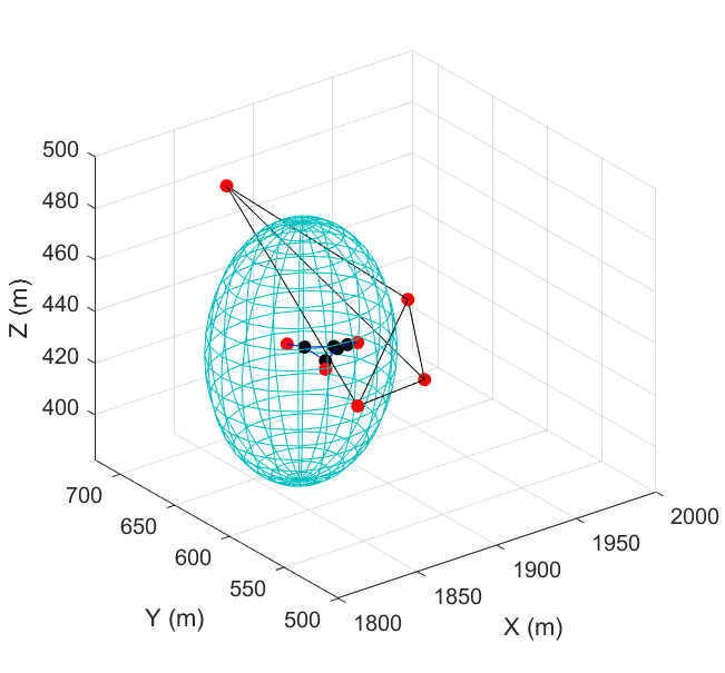
The safety condition (33a) is necessary but not sufficient for ensuring of the MQS collision avoidance with obstacles. Fig. 1 illustrates a situation in which collision is not avoided because the safety condition (33b) is violated while (33a) is satisfied. More specifically, Fig. 1 shows that vertices of a tetrahedron enclosing an obstacle are outside of containment ball $\mathcal{S}$ , where $\mathcal{S}$ contains the MQS. However, the containment ball enclosing the MQS is contained by the tetrahedron representing obstacle in the motion space.

Refer to caption — Figure 1: Violation of collision avoidance requirements: MQS leaders are contained by the containment ball while the tetrahedron, representing an obstacle, encloses the containment ball in the motion space.

IV-A2 A* Optimizer Functionality

To plan the desired coordination of the MQS, we represent the coordination space by a finite number of nodes obtained by uniform discretization of the motion space. Let $\mathcal{D}_{x}=\left\{\Delta x,2\Delta x,\cdots,n_{x}\Delta x\right\}$ , $\mathcal{D}_{y}=\left\{\Delta y,2\Delta y,\cdots,n_{y}\Delta x\right\}$ , and $\mathcal{D}_{z}=\left\{\Delta z,2\Delta z,\cdots,n_{z}\Delta z\right\}$ define all possible discrete values for the $x$ , $y$ , and $z$ components of the nodes distributed in the motion space. Then,

$\mathcal{D}=\left\{\tilde{\mathbf{d}}=\left(\tilde{d}_{x}\Delta x,\tilde{d}_{y}\Delta y,\tilde{d}_{z}\Delta z\right):\tilde{d}_{x}\Delta x\in\mathcal{D}_{x},\tilde{d}_{y}\Delta y\in\mathcal{D}_{y},\tilde{d}_{z}\Delta z\in\mathcal{D}_{z}\right\}$

(34)

defines positions of the nodes in the motion space.

Assumption 3.

The containment polytopes enclosing obstacles are defined such that $\mathcal{P}\subset\mathcal{D}$ .

Definition 3.

We define

\begin{split}\mathcal{F}=&\bigg\{\tilde{\mathbf{d}}\in\mathcal{D}:\left(\bigwedge_{j\in\mathcal{P}}\bigwedge_{l=1}^{m_{j}}\bigwedge_{p\in\mathcal{T}_{j,l}}\left(\left(x_{p},y_{p},z_{p}\right)\notin\mathcal{S}\left(\tilde{\mathbf{d}},r_{\mathrm{max}}\right)\right)\right)\wedge\\ &\left(\bigwedge_{j\in\mathcal{P}}\bigwedge_{l=1}^{m_{j}}\bigwedge_{\mathcal{T}_{j,l}=\left\{v_{1},\cdots,v_{4}\right\}}\left(\mathbf{\Omega}_{3}\left(\mathbf{p}_{v_{1}},\mathbf{p}_{v_{2}},\mathbf{p}_{v_{3}},\mathbf{p}_{v_{4}},\mathbf{r}\right)\not\geq\mathbf{0}\right)\right),\penalty\ \\ &\mathrm{for\penalty\ }\mathbf{r}\in\partial\mathcal{S}\left(\tilde{\mathbf{d}},r_{\mathrm{max}}\right)\bigg\}\subset\mathcal{D}\end{split}

(35)

as the set of valid positions for the center of ball $\mathcal{S}$ .

Assumption 4.

Initial and final positions of the containment ball are defined such that $\bar{\mathbf{d}}_{s}\in\mathcal{F}$ and $\bar{\mathbf{d}}_{n_{\tau}}\in\mathcal{F}$ .

Definition 4.

Set

$\mathcal{A}\left(\tilde{\mathbf{d}}\right)=\left\{\left(\tilde{\mathbf{d}}+\left(h_{x}\Delta_{x},h_{y}\Delta_{y},h_{z}\Delta_{z}\right)\right)\in\mathcal{F}:h_{x},h_{y},h_{z}\in\{-1,0,1\}\right\}$

(36)

defines all possible valid neighboring points of point $\tilde{\mathbf{d}}\in\mathcal{F}$ .

Definition 5.

For every $\tilde{\mathbf{d}}\in\mathcal{F}$ , the straight line distance

C_{H}\left(\tilde{\mathbf{d}},\bar{\mathbf{d}}_{u}\right)=\|\tilde{\mathbf{d}}-\bar{\mathbf{d}}_{u}\|

(37)

is considered as the heuristic cost of position vector $\tilde{\mathbf{d}}\in\mathcal{F}$ .

Definition 6.

For every $\tilde{\mathbf{d}}\in\mathcal{F}$ and $\tilde{\mathbf{d}}^{\prime}\in\mathcal{A}\left(\tilde{\mathbf{d}}\right)$ ,

C_{O}\left(\tilde{\mathbf{d}},\tilde{\mathbf{d}}^{\prime}\right)=\|\tilde{\mathbf{d}}-\tilde{\mathbf{d}}^{\prime}\|

(38)

is the operation cost for the movement from $\tilde{\mathbf{d}}\in\mathcal{F}$ towards $\tilde{\mathbf{d}}^{\prime}\in\mathcal{A}\left(\tilde{\mathbf{d}}\right)$ .

Algorithm 1 A* Planning of the MQS Coordination

1: Get:

\bar{\mathbf{d}}_{s}

and

\bar{\mathbf{d}}_{u}

2: Define: Open set

\mathcal{O}=\left\{\bar{\mathbf{d}}_{s}\right\}

, Closed set

\mathcal{C}=\emptyset

, and

\tilde{\mathbf{d}}_{\mathrm{best}}=\bar{\mathbf{d}}_{s}

3: while

\tilde{\mathbf{d}}_{\mathrm{best}}=\bar{\mathbf{d}}_{u}

\mathcal{O}\neq\emptyset

\tilde{\mathbf{d}}_{\mathrm{best}}\leftarrow\argmin\limits_{\tilde{\mathbf{d}}\in\mathcal{F}}\left(g\left(\tilde{\mathbf{d}}\right)+C_{H}\left(\tilde{\mathbf{d}},\bar{\mathbf{d}}_{u}\right)\right)

5: Update

\mathcal{O}

\mathcal{O}\leftarrow\mathcal{O}\setminus\left\{\tilde{\mathbf{d}}_{\mathrm{best}}\right\}

6: Update

\mathcal{C}

\mathcal{C}\leftarrow\mathcal{C}\bigcup\left\{\tilde{\mathbf{d}}_{\mathrm{best}}\right\}

7: Assign

\mathcal{A}\left(\tilde{\mathbf{d}}_{\mathrm{best}}\right)

\mathcal{R}\left(\tilde{\mathbf{d}}_{\mathrm{best}}\right)\leftarrow\mathcal{A}\left(\tilde{\mathbf{d}}_{\mathrm{best}}\right)\setminus\left(\mathcal{A}\left(\tilde{\mathbf{d}}_{\mathrm{best}}\right)\bigcap\mathcal{C}\right)

9: for < every

\tilde{\mathbf{d}}\in\mathcal{R}\left(\tilde{\mathbf{d}}_{\mathrm{best}}\right)

> do

10:

\tilde{\mathbf{b}}\left(\tilde{\mathbf{d}}\right)\leftarrow\tilde{\mathbf{d}}

11: if

\tilde{\mathbf{d}}\in\mathcal{O}

then

12: if

g\left(\tilde{\mathbf{d}}_{\mathrm{best}}\right)+C_{O}\left(\tilde{\mathbf{d}}_{\mathrm{best}},\tilde{\mathbf{d}}\right)<g\left(\tilde{\mathbf{d}}\right)

then

13:

g\left(\tilde{\mathbf{d}}\right)\leftarrow g\left(\tilde{\mathbf{d}}_{\mathrm{best}}\right)+C_{O}\left(\tilde{\mathbf{d}}_{\mathrm{best}},\tilde{\mathbf{d}}\right)

14:

\tilde{\mathbf{b}}\left(\tilde{\mathbf{d}}\right)\leftarrow\tilde{\mathbf{d}}_{\mathrm{best}}

15: end if

16: end if

17: end for

18:

\mathcal{O}\leftarrow\mathcal{R}\left(\tilde{\mathbf{d}}_{\mathrm{best}}\right)\bigcup\mathcal{O}

19: end while

Given initial and final locations of the center of the containment ball $\mathcal{S}$ , denoted by $\bar{\mathbf{d}}_{s}$ and $\bar{\mathbf{d}}_{u}$ , the A* search algorithm is applied to determine optimal intermediate positions $\bar{\mathbf{b}}_{s}$ , $\cdots$ , $\bar{\mathbf{b}}_{m_{\tau}}$ along the optimal path of the containment ball $\mathcal{S}$ from $\bar{\mathbf{d}}_{s}$ to $\bar{\mathbf{d}}_{u}$ in an obstacle-laden environment (See Algorithm 1). More specifically, the A* optimizer generates $\bar{\mathbf{b}}_{s}$ , $\cdots$ , $\bar{\mathbf{b}}_{m_{\tau}}$ by searching over set $\mathcal{F}$ , where

	$\bar{\mathbf{b}}_{s}=\bar{\mathbf{d}}_{s},$		(39a)
	$\bar{\mathbf{b}}_{m_{\tau}}=\bar{\mathbf{d}}_{u},$		(39b)
	$\left(\bar{\mathbf{b}}_{k},\bar{\mathbf{b}}_{k+1}\right)\in\mathcal{A}\left(\bar{\mathbf{b}}_{k}\right).$		(39c)

The center of the containment ball $\mathcal{S}$ moves along the straight paths obtained by connecting $\bar{\mathbf{b}}_{s}$ , $\cdots$ , $\bar{\mathbf{b}}_{m_{\tau}}$ . Therefore, $n_{\tau}$ serially-connected line segments defines the optimal path of the containment ball, where $n_{\tau}\leq m_{\tau}$ , $\bar{\mathbf{d}}_{s}=\bar{\mathbf{b}}_{s}$ , $\bar{\mathbf{d}}_{n_{\tau}}=\bar{\mathbf{b}}_{m_{\tau}}=\bar{\mathbf{d}}_{u}$ , and the end point of the $k$ -th line segment connects $\bar{\mathbf{d}}_{k-1}$ to $\bar{\mathbf{d}}_{k}$ . Given $\bar{\mathbf{b}}_{s}$ , $\cdots$ , $\bar{\mathbf{b}}_{m_{\tau}}$ , algorithm 2 is used to determine $\bar{\mathbf{d}}_{1}$ , $\cdots$ , $\bar{\mathbf{d}}_{n_{\tau}-1}$ .

Algorithm 2 Assignment of Optimal Way-points

\bar{\mathbf{d}}_{1}

\cdots

\bar{\mathbf{d}}_{n_{\tau}-1}

1: Get:

\bar{\mathbf{b}}_{s}=\bar{\mathbf{d}}_{s}

\cdots

\bar{\mathbf{b}}_{m_{\tau}}=\bar{\mathbf{d}}_{u}

2: Set:

i=0

3: for <

k\leftarrow 1

m_{\tau}-1

> do

4: if

\bar{\mathbf{b}}_{k}-\bar{\mathbf{b}}_{k-1}\neq\bar{\mathbf{b}}_{k+1}-\bar{\mathbf{b}}_{k}

then

i\leftarrow i+1

\bar{\mathbf{d}}_{i}=\bar{\mathbf{b}}_{k}

7: end if

8: end for

IV-B Intermediate Configuration of the Leading Triangle

Matrix $\mathbf{Q}_{xy}(t)$ can be expressed by

\mathbf{Q}_{xy}(t)=\mathbf{R}_{xy}(t)\mathbf{U}_{xy}(t),

(40)

where rotation matrix $\mathbf{R}_{xy}(t)$ and pure deformation matrix $\mathbf{U}_{xy}(t)$ are defined as follows:

	$\mathbf{R}_{xy}(t)=\begin{bmatrix}\cos\theta_{r}&-\sin\theta_{r}\\ \sin\theta_{r}&\cos\theta_{r}\end{bmatrix},$		(41a)
	$\mathbf{U}_{xy}(t)=\mathbf{R}_{D}(t)\mathbf{\Lambda}(t)\mathbf{R}_{D}^{T}(t),$		(41b)

where

	$\mathbf{\Lambda}(t)=\begin{bmatrix}\sigma_{1}(t)&0\\ 0&\sigma_{2}(t)\end{bmatrix},$		(42a)
	$\mathbf{R}_{D}(t)=\begin{bmatrix}\cos\theta_{d}&-\sin\theta_{d}\\ \sin\theta_{d}&\cos\theta_{d}\end{bmatrix}.$		(42b)

Note that $\theta_{r}(t)>0$ and $\theta_{d}(t)>0$ are the rotation and shear deformation angles; and $\sigma_{1}(t)$ and $\sigma_{2}(t)$ are the first and second deformation eigenvalues. Because $\mathbf{\Lambda}(t)$ is positive definite and diagonal, matrix $\mathbf{U}_{xy}(t)$ is positive definite at any time $t\in\left[t_{s},t_{u}\right]$ [24].

Proposition 1.

Matrix $\mathbf{U}_{xy}^{m}$ can be expressed as

\mathbf{U}_{xy}^{m}(t)=\begin{bmatrix}a_{m}(t)&b_{m}(t)\\ b_{m}(t)&a_{m}(t)\end{bmatrix},

(43)

with

	$a_{m}(t)=\sigma_{1}^{m}(t)\cos^{2}\theta_{d}(t)+\sigma_{2}^{m}(t)\sin^{2}\theta_{d}(t),$		(44a)
	$b_{m}(t)=\left(\sigma_{1}^{m}(t)-\sigma_{2}^{m}(t)\right)\sin\theta_{d}(t)\cos\theta_{d}(t),$		(44b)
	$c_{m}(t)=\sigma_{1}^{m}(t)\sin^{2}\theta_{d}(t)+\sigma_{2}^{m}(t)\cos^{2}\theta_{d}(t).$		(44c)

Also, $\sigma_{1}$ , $\sigma_{2}$ , and $\theta_{d}$ can be related to $a_{m}$ , $b_{m}$ , and $c_{m}$ by

	$\sigma_{1}(t)=\sqrt[m]{\dfrac{a_{m}(t)+c_{m}(t)}{2}+\sqrt{\big[{1\over 2}\left(a_{m}(t)-c_{m}(t)\right)\big]^{2}+b_{m}^{2}(t)}},$		(45a)
	$\sigma_{2}(t)=\sqrt[m]{\dfrac{a_{m}(t)+c_{m}(t)}{2}-\sqrt{\big[{1\over 2}\left(a_{m}(t)-c_{m}(t)\right)\big]^{2}+b_{m}^{2}(t)}},$		(45b)
	$\theta_{d}(t)=\dfrac{1}{2}\tan^{-1}\left(\dfrac{2b_{m}(t)}{a_{m}(t)-c_{m}(t)}\right).$		(45c)

Proof.

Because $\mathbf{R}_{D}(t)$ is orthogonal at time $t$ , $\mathbf{R}_{D}^{T}(t)\mathbf{R}_{D}(t)=\mathbf{I}_{2}$ . If matrix $\mathbf{U}_{xy}^{m}$ is expressed as

\mathbf{U}_{xy}^{m}(t)=\mathbf{R}_{D}(t)\mathbf{\Lambda}^{m}\mathbf{R}_{D}(t),

(46)

for $m=1,2,\cdots$ , then,

\begin{split}\mathbf{U}_{xy}^{m+1}(t)=&\mathbf{R}_{D}(t)\mathbf{\Lambda}\mathbf{R}_{D}^{T}(t)\mathbf{R}_{D}(t)\mathbf{\Lambda}^{m}\mathbf{R}_{D}(t)\\ =&\mathbf{R}_{D}(t)\mathbf{\Lambda}^{m+1}\mathbf{R}_{D}(t).\end{split}

(47)

Since Eq. (46) is valid for $m=0$ , Eq. (47) ensures that Eq. (46) is valid for any $m>0$ . By replacing (42a) and (42b) into (46), elements of matrix $\mathbf{U}_{xy}^{m}$ ( $a_{m}$ , $b_{m}$ , $c_{m}$ ) are obtained by Eqs. (44a), (44b), and (44c). ∎

By provoking Proposition 1, matrix $\mathbf{U}_{xy}^{2}=\mathbf{Q}_{xy}^{T}\mathbf{Q}_{xy}$ [24] can be expressed in the form of Eq. (43) where $m=2$ and

	$a_{2}(t)=\mathbf{y}_{L,HT}^{T}(t)\mathbf{O}^{T}\mathbf{\Gamma}^{T}\left(\mathbf{E}_{1}^{T}\mathbf{E}_{1}+\mathbf{E}_{3}^{T}\mathbf{E}_{3}\right)\mathbf{\Gamma}\mathbf{O}\mathbf{y}_{L,HT}(t),$		(48a)
	$b_{2}(t)=\mathbf{y}_{L,HT}^{T}(t)\mathbf{O}^{T}\mathbf{\Gamma}^{T}\left(\mathbf{E}_{1}^{T}\mathbf{E}_{2}+\mathbf{E}_{3}^{T}\mathbf{E}_{4}\right)\mathbf{\Gamma}\mathbf{O}\mathbf{y}_{L,HT}(t),$		(48b)
	$c_{2}(t)=\mathbf{y}_{L,HT}^{T}(t)\mathbf{O}^{T}\mathbf{\Gamma}^{T}\left(\mathbf{E}_{2}^{T}\mathbf{E}_{2}+\mathbf{E}_{4}^{T}\mathbf{E}_{4}\right)\mathbf{\Gamma}\mathbf{O}\mathbf{y}_{L,HT}(t).$		(48c)

Therefore, we can determine $\sigma_{1}(t)$ , $\sigma_{2}(t)$ , and $\theta_{d}(t)$ by replacing $m=2$ , $a_{m}(t)=a_{2}(t)$ , $b_{m}(t)=b_{2}(t)$ , and $c_{m}(t)=c_{2}(t)$ into Eqs. (45a), (45b), and (45c) at time $t\in\left[t_{s},t_{u}\right]$ . Furthermore, matrix $\mathbf{R}_{xy}(t)=\mathbf{Q}\mathbf{U}_{xy}^{-1}$ is related to $\mathbf{y}_{L,HT}(t)$ by

\mathbf{R}_{xy}(t)=\begin{bmatrix}\mathbf{E}_{1}\mathbf{\Gamma}\mathbf{O}\mathbf{y}_{L,HT}(t)&\mathbf{E}_{2}\mathbf{\Gamma}\mathbf{O}\mathbf{y}_{L,HT}(t)\\ \mathbf{E}_{3}\mathbf{\Gamma}\mathbf{O}\mathbf{y}_{L,HT}(t)&\mathbf{E}_{4}\mathbf{\Gamma}\mathbf{O}\mathbf{y}_{L,HT}(t)\\ \end{bmatrix}\begin{bmatrix}a_{2}(t)&b_{2}(t)\\ b_{2}(t)&c_{2}(t)\end{bmatrix}^{-1\over 2}.

(49)

Therefore, rotation angle $\theta_{r}(t)$ is obtained at any time $t\in\left[t_{s},t_{u}\right]$ by knowing rotation matrix $\mathbf{R}_{xy}(t)$ over time interval $\left[t_{s},t_{u}\right]$ .

Proposition 2.

If the area of the leading triangle remains constant at any time $t\in[t_{s},t_{u}]$ , then the following conditions hold:

	$\sigma_{2}(t)={1\over\sigma_{1}(t)},$		(50a)
	$a_{2}(t)c_{2}(t)-b_{2}{{}^{2}}=1.$		(50b)

Proof.

Per Assumption 2, $\mathbf{U}_{xy}(t_{s})=\mathbf{I}_{2}$ . If the area of the leading triangle remains constant, then $\sigma_{1}(t)\sigma_{2}(t)=\sigma_{1}(t_{s})\sigma_{2}(t_{s})=1$ and $\left|\mathbf{U}_{xy}(t)\right|{\color[rgb]{0,0,0}=a_{2}(t)c_{2}(t)-b_{2}^{2}}=1$ at any time $t$ . Therefore, conditions (50a) and (50b) hold at any time $t\in\left[t_{s},t_{u}\right]$ . ∎

Theorem 2.

Assume every quadcopter $i\in\mathcal{V}$ can be enclosed by a ball of radius $\epsilon$ , and it can execute a proper control input $\mathbf{u}_{i}$ such that

\bigwedge_{i\in\mathcal{V}}\|\mathbf{r}_{i}(t)-\mathbf{p}_{i}(t)\|\leq\delta,\qquad\forall t\in\left[t_{s},t_{u}\right].

(51)

Let

d_{\mathrm{min}}=\min\limits_{i,j\in\mathcal{V},\penalty\ j\neq i}\left\|\mathbf{p}_{i,0}-\mathbf{p}_{j,o}\right\|,

(52)

be the minimum separation distance between two quadcopters. Then, collision between every two quadcopers and collision of the MQS with obstacles are both avoided, if the largest eigenvalue of matrix $\mathbf{U}_{xy}$ satisfies inequality constraint

\sigma_{1}(t)\leq\dfrac{d_{\mathrm{min}}}{2\left(\delta+\epsilon\right)},

(53)

and every quadcopter remains inside the containment ball $\mathcal{S}\left(\mathbf{d}\left(t\right),r_{\mathrm{max}}\right)$ at any time $t\in\left[t_{s},t_{u}\right]$ .

Proof.

Per Eqs. (45a) and (45b), $\sigma_{2}(t)\leq\sigma_{1}(t)$ at any time $t\in\left[t_{s},t_{u}\right]$ . Collision between every two quadcopters is avoided, if [24]

\sigma_{2}(t)\geq{2\left(\delta+\epsilon\right)\over d_{\mathrm{min}}},\qquad\forall t\in\left[t_{s},t_{u}\right].

(54)

Per Proposition 2, $\sigma_{2}(t)={1\over\sigma_{1}(t)}$ . Thus, Eq. (54) can be rewritten as follows:

\sigma_{1}(t)\leq{2\left(\delta+\epsilon\right)\over d_{\mathrm{min}}},\qquad\forall t\in\left[t_{s},t_{u}\right].

(55)

By applying A* search method, we ensure that the containment ball does not hit obstacles in the motion space. Therefore, obstacle collision avoidance is guaranteed, if quadcopters are all inside the containment ball $\mathcal{S}\left(\mathbf{d}\left(t\right),r_{\mathrm{max}}\right)$ at any time $t\in\left[t_{s},t_{u}\right]$ . ∎

Intermediate Configurations Leaders: We offer a procedure with the following five main steps to determine the intermediate waypoints of the leaders:

Step 1: Given $\bar{\mathbf{y}}_{L,HT,n_{\tau}}=\mathbf{y}_{L,HT}\left(t_{u}\right)$ , $\sigma_{1,n_{\tau}}=\sigma_{1}(t_{u})$ , $\theta_{d,n_{\tau}}=\theta_{d}(t_{u})$ , and $\theta_{r,n_{\tau}}=\theta_{r}(t_{u})$ are computed using Eqs. (45a), (45c), and (49), respectively.

Step 2: We compute

	$\sigma_{1,k}=\beta_{k}\sigma_{1,0}+(1-\beta_{k})\sigma_{1,n_{\tau}},$		(56a)
	$\theta_{d,k}=(1-\beta_{k})\theta_{d,n_{\tau}},$		(56b)
	$\theta_{r,k}=(1-\beta_{k})\theta_{r,n_{\tau}}$		(56c)

for $k=1,\cdots,n_{\tau}-1$ , where $\beta_{k}$ is computed using Eq. (12).

Step 3: We compute $\sigma_{2,k}={1\over\sigma_{1,k}}$ for $k=1,\cdots,n_{\tau}-1$ .

Step 4: Given $\sigma_{1,k}$ , $\sigma_{2,k}$ , and $\theta_{d,k}$ , matrix $\mathbf{U}_{xy,k}=\mathbf{U}_{xy}\left(t_{k}\right)$ is obtained by Eq. (41b) for $k=1,\cdots,n_{\tau}-1$ . Also, matrix $\mathbf{R}_{xy,k}=\mathbf{R}_{xy}\left(t_{k}\right)$ is obtained using Eq. (41a) by knowing the rotation angle $\theta_{r,k}$ for $k=1,\cdots,n_{\tau}-1$ .

Step 5: By knowing $\mathbf{R}_{xy,k}=\mathbf{R}_{xy}\left(t_{k}\right)$ and $\mathbf{U}_{xy,k}=\mathbf{U}_{xy}\left(t_{k}\right)$ , the Jacobian matrix $\mathbf{Q}_{xy,k}=\mathbf{Q}_{xy}\left(t_{k}\right)$ is obtained using Eq. (40). Then, we can use relation (20) to obtain $\bar{\mathbf{y}}_{L,HT,k}$ by replacing $\mathbf{Q}_{xy,k}=\mathbf{Q}_{xy}\left(t_{k}\right)$ and $\bar{\mathbf{d}}_{k}$ for $k=1,\cdots,n_{\tau}-1$ .

IV-C Optimal Control Planning

This section offers an optimal control solution to determine the leaders’ desired trajectories connecting every two consecutive waypoints $\bar{\mathbf{y}}_{L,HT,k}$ and $\bar{\mathbf{y}}_{L,HT,k+1}$ for $k=0,1,\cdots,n_{\tau}-1$ , where $z$ components of the leaders is defined by Eq. (14), and $x$ and $y$ components the leaders’ desired trajectories are governed by (16).

Coordination Constraint: Per equality constraint (9a), the area of the leading triangle, given by

A(t)=\mathbf{y}_{L,HT}^{T}(t)\mathbf{\Psi}\mathbf{y}_{L,HT}(t),

(57)

must be equal to constant value $A_{s}$ at any time $t\in\left[t_{s},t_{u}\right]$ . This equality constraint is satisfied, if $\mathbf{y}_{L,HT}(t)$ is updated by dynamics (16), $c\left(\mathbf{x}_{L},\mathbf{u}_{L}\right)=\ddot{A}\left(t\right)=0$ at any time $t\in\left[t_{k},t_{k+1}\right]$ for $k=0,1,\cdots,n_{\tau}-1$ , and the following boundary conditions are satisfied:

	$k=0,1,\cdots,n_{\tau},\qquad{\mathbf{y}}_{L,HT}^{T}\left(t_{k}\right)\mathbf{D}^{T}\mathbf{O}^{T}\mathbf{P}^{T}\mathbf{P}\mathbf{O}\mathbf{D}\mathbf{y}_{L,HT}\left(t_{k}\right)-A_{s}=0,$		(58a)
	$k=0,1,\cdots,n_{\tau},\qquad\dot{\mathbf{y}}_{L,HT}^{T}\left(t_{k}\right)\mathbf{D}^{T}\mathbf{O}^{T}\mathbf{P}^{T}\mathbf{P}\mathbf{O}\mathbf{D}\mathbf{y}_{L,HT}\left(t_{k}\right)=0.$		(58b)

By taking the second time derivative of ${A}\left(t\right)$ , $c\left(\mathbf{x}_{L},\mathbf{u}_{L}\right)$ is obtained as follows:

c\left(\mathbf{x}_{L},\mathbf{u}_{L},t\right)=\mathbf{x}_{L}^{T}\mathbf{\Gamma}_{\mathbf{xx}}\mathbf{x}_{L}+2\mathbf{x}_{L}^{T}\mathbf{\Gamma}_{\mathbf{xu}}\mathbf{u}_{L}=0,

(59)

where

	$\mathbf{\Gamma}_{\mathbf{xx}}=2\begin{bmatrix}\mathbf{0}_{6\times 6}&\mathbf{P}\\ \mathbf{P}&\mathbf{0}_{6\times 6}\\ \end{bmatrix},$		(60a)
	$\mathbf{\Gamma}_{\mathbf{xu}}=\begin{bmatrix}\mathbf{P}\\ \mathbf{0}_{6\times 6}\\ \end{bmatrix}.$		(60b)

The objective of the optimal control planning is to determine the desired trajectories of the leaders by minimization of cost function

k=0,1,\cdots,n_{\tau}-1,\qquad\mathrm{J}={1\over 2}\int_{t_{k}\left(t_{u}\right)}^{t_{k+1}\left(t_{u}\right)}\mathbf{u}_{L}^{T}(t)\mathbf{u}_{L}^{T}(t)dt

(61)

subject to boundary conditions

	$\mathbf{x}_{L}(t_{k})=\bar{\mathbf{x}}_{L,k},$		(62a)
	$\mathbf{x}_{L}(t_{k+1})=\bar{\mathbf{x}}_{L,k+1},$		(62b)

and equality constraint (59) at any time $t\in\left[t_{k}\left(t_{u}\right),t_{k+1}\left(t_{u}\right)\right]$ for $k=0,1,\cdots,n_{\tau}-1$ where $t_{k}(t_{u})$ is obtained by (13).

Theorem 3.

Suppose leaders’ desired trajectories are updated by dynamics (16) such that equality constraint (59) is satisfied at any time $t\in\left[t_{k}\left(t_{u}\right),t_{k+1}\left(t_{u}\right)\right]$ given the boundary conditions in Eq. (62). Assuming the ultimate time $t_{u}$ is given, $t_{k}$ and $t_{k+1}$ obtained by Eq. (13) are fixed, and the optimal desired trajectories of leaders minimizing the cost function (61) are governed by dynamics

\begin{bmatrix}\dot{\mathbf{x}}_{L}\\ \dot{\lambda}\end{bmatrix}=\mathbf{A}_{\mathbf{x\lambda}}\left(\gamma(t)\right)\begin{bmatrix}{\mathbf{x}}_{L}\\ {\lambda}\end{bmatrix},

(63)

where

	$\mathbf{A}_{\mathbf{x\lambda}}\left(\gamma(t)\right)=\begin{bmatrix}\mathbf{A}_{L}-2\gamma(t)\mathbf{B}_{L}\mathbf{\Gamma}_{\mathbf{xu}}^{T}&-\mathbf{B}_{L}\mathbf{B}_{L}^{T}\\ -2\gamma\mathbf{\Gamma}_{\mathbf{xx}}+4\gamma^{2}(t)\mathbf{\Gamma}_{\mathbf{xu}}\mathbf{\Gamma}_{\mathbf{xu}}^{T}&-\mathbf{A}_{L}^{T}+2\gamma(t)\mathbf{\Gamma}_{\mathbf{xu}}\mathbf{B}_{L}^{T}\\ \end{bmatrix},$		(64a)
	$\gamma\left(t\right)=\dfrac{\mathbf{x}_{L}^{T}\mathbf{\Gamma}_{\mathbf{xx}}\mathbf{x}_{L}+\mathbf{\Gamma}_{\mathbf{x}}^{T}\mathbf{x}_{L}-2\mathbf{x}_{L}^{T}\mathbf{\Gamma}_{\mathbf{xu}}\mathbf{B}_{L}^{T}\mathbf{\lambda}}{4\mathbf{x}_{L}^{T}\mathbf{\Gamma}_{\mathbf{xu}}\mathbf{\Gamma}_{\mathbf{xu}}^{T}\mathbf{x}_{L}},$		(64b)

and $\lambda\in\mathbb{R}^{18\times 1}$ is the co-state vector. In addition, the state vector $\mathbf{x}_{L}(t)$ and co-state vector $\lambda(t)$ are obtained by

	$\begin{split}\mathbf{x}_{L}(t)=&\left(\mathbf{\Phi}_{11}\left(t,t_{k}\right)-\mathbf{\Phi}_{12}\left(t,t_{k+1}\right)\mathbf{\Phi}_{11}\left(t_{k+1},t_{k}\right)\right)\bar{\mathbf{x}}_{L,k}\\ +&\mathbf{\Phi}_{12}\left(t,t_{k+1}\right)\bar{\mathbf{x}}_{L,k+1}\end{split}$		(65a)
	$\begin{split}\lambda(t)=&\left(\mathbf{\Phi}_{21}\left(t,t_{k}\right)-\mathbf{\Phi}_{22}\left(t,t_{k+1}\right)\mathbf{\Phi}_{11}\left(t_{k+1},t_{k}\right)\right)\bar{\mathbf{x}}_{L,k}\\ +&\mathbf{\Phi}_{22}\left(t,t_{k+1}\right)\bar{\mathbf{x}}_{L,k+1}\end{split}$		(65b)

at time $t\in\left[t_{k},t_{k+1}\right]$ , where

\mathbf{\Phi}=\begin{bmatrix}\mathbf{\Phi}_{11}\left(t,t_{k}\right)&\mathbf{\Phi}_{12}\left(t,t_{k}\right)\\ \mathbf{\Phi}_{21}\left(t,t_{k}\right)&\mathbf{\Phi}_{22}\left(t,t_{k}\right)\\ \end{bmatrix}=\mathrm{exp}\left(\int_{t_{k}}^{t}\mathbf{A}_{\mathbf{x\lambda}}\left(\gamma(s)\right)ds\right)

(66)

is the state transition matrix with partitions $\mathbf{\Phi}_{11}\left(t,t_{k}\right)\in\mathbb{R}^{12\times 12}$ , $\mathbf{\Phi}_{12}\left(t,t_{k}\right)\in\mathbb{R}^{12\times 12}$ , $\mathbf{\Phi}_{21}\left(t,t_{k}\right)\in\mathbb{R}^{12\times 12}$ , and $\mathbf{\Phi}_{22}\left(t,t_{k}\right)\in\mathbb{R}^{12\times 12}$ .

Proof.

The optimal leaders’ trajectories are determined by minimization of the augmented cost function

$\mathrm{J}_{a}=\int_{t_{k}}^{t_{k+1}}\left({1\over 2}\mathbf{u}_{L}^{T}\mathbf{u}_{L}^{T}+\mathbf{\lambda}^{T}\left(\mathbf{A}_{L}{\mathbf{x}}_{L}+\mathbf{B}_{L}{\mathbf{u}}_{L}-\dot{\mathbf{x}}_{L}\right)+\gamma c\left(\mathbf{x}_{L},\mathbf{u}_{L}\right)\right)dt,$

(67)

where $\mathbf{\lambda}\in\mathbb{R}^{12\times 1}$ is the co-state vector and $\gamma(t)$ is the Lagrange multiplier. By taking variation from the augmented cost function (67), we can write

\begin{split}\delta\mathrm{J}_{a}=\int_{t_{k}}^{t_{k+1}}&\Bigg[\delta\mathbf{u}_{L}^{T}\left(\mathbf{u}_{L}+\mathbf{B}_{L}^{T}\mathbf{\lambda}+\gamma{\partial c\over\partial\mathbf{u}_{L}}\right)+\delta\mathbf{x}_{L}^{T}\left(\dot{\mathbf{\lambda}}+\mathbf{A}_{L}^{T}\mathbf{\lambda}+\gamma{\partial c\over\partial\mathbf{x}_{L}}\right)\\ +&\delta\mathbf{\lambda}^{T}\left(\mathbf{A}_{L}{\mathbf{x}}_{L}+\mathbf{B}_{L}{\mathbf{u}}_{L}-\dot{\mathbf{x}}_{L}\right)\bigg]dt=0,\end{split}

(68)

where ${\partial c\over\partial\mathbf{x}_{L}}=2\mathbf{\Gamma}_{\mathbf{xx}}\mathbf{x}_{L}+2\mathbf{\Gamma}_{\mathbf{xu}}\mathbf{u}_{L}$ and ${\partial c\over\partial\mathbf{u}_{L}}=2\mathbf{\Gamma}_{\mathbf{xu}}^{T}\mathbf{x}_{L}$ . By imposing $\delta\mathrm{J}_{a}=0$ , the state dynamics (16) is obtained, the co-state dynamics become

\dot{\mathbf{\lambda}}=-\mathbf{A}_{L}^{T}\mathbf{\lambda}-\gamma(t)\dfrac{\partial c}{\partial\mathbf{x}_{L}},

(69)

and $\mathbf{u}_{L}$ is obtained as follows:

\mathbf{u}_{L}=-\mathbf{B}_{L}^{T}\mathbf{\lambda}-\gamma{\partial c\over\partial\mathbf{u}_{L}}=-\mathbf{B}_{L}^{T}\mathbf{\lambda}-2\gamma(t)\mathbf{\Gamma}_{\mathbf{xu}}^{T}\mathbf{x}_{L}.

(70)

By substituting $\mathbf{u}_{L}=-\mathbf{B}_{L}^{T}\mathbf{\lambda}-2\gamma(t)\mathbf{\Gamma}_{\mathbf{xu}}\mathbf{x}_{L}$ , the equality constraint (59) is converted to

c\left(\mathbf{x}_{L},\mathbf{u}_{L}\right)=\left(4\mathbf{x}_{L}^{T}\mathbf{\Gamma}_{\mathbf{xu}}\mathbf{\Gamma}_{\mathbf{xu}}^{T}\mathbf{x}_{L}\right)\gamma(t)+\mathbf{x}_{L}^{T}\mathbf{\Gamma}_{\mathbf{xx}}\mathbf{x}_{L}-2\mathbf{x}_{L}^{T}\mathbf{\Gamma}_{\mathbf{xu}}\mathbf{B}_{L}^{T}\mathbf{\lambda}=0.

(71)

By substituting $\mathbf{u}_{L}=-\mathbf{B}_{L}^{T}\mathbf{\lambda}-2\gamma(t)\mathbf{\Gamma}_{\mathbf{xu}}\mathbf{x}_{L}-\gamma\mathbf{\mathbf{\Gamma}}_{u}$ into Eq. (16), we also obtain the leaders’ desired trajectories solving dynamics (63). The solution of dynamics (63) is given by

\begin{bmatrix}{\mathbf{x}}_{L}(t)\\ {\lambda}(t)\end{bmatrix}=\begin{bmatrix}\mathbf{\Phi}_{11}\left(t,t_{k}\right)&\mathbf{\Phi}_{12}\left(t,t_{k}\right)\\ \mathbf{\Phi}_{21}\left(t,t_{k}\right)&\mathbf{\Phi}_{22}\left(t,t_{k}\right)\\ \end{bmatrix}\begin{bmatrix}\bar{\mathbf{x}}_{L,k}\\ {\lambda}_{k}\end{bmatrix}

(72)

at time $t\in[t_{k},t_{k+1}]$ , where ${\lambda}_{k}=\lambda\left(t_{k}\right)$ . By imposition boundary condition (62b),

\lambda_{k}=\mathbf{\Phi}_{12}\left(t_{k},t_{k+1}\right)\left(\mathbf{x}_{L}\left(t_{k+1}\right)-\mathbf{\Phi}_{11}\left(t_{k+1},t_{k}\right)\mathbf{x}_{L}\left(t_{k}\right)\right)

(73)

is obtained from Eq. (72). By substituting $\lambda_{k}$ into Eq. (72), $\mathbf{x}_{L}(t)$ is obtained by Eq. (65a) at any time $t\in\left[t_{k},t_{k+1}\right]$ .

∎

Algorithm 3 Assignment of travel time

t_{u}

and desired trajectory

\mathbf{x}_{L}(t)

over

\left[t_{0},t_{u}\right]

1: Get:

\bar{\mathbf{x}}_{L,0}

\cdots

\bar{\mathbf{x}}_{L,n_{\tau}}

and

\beta_{0}

\cdots

\beta_{n_{\tau}-1}

\epsilon_{T}

\epsilon_{\gamma}

, small

T_{\mathrm{min}}

and large

T_{\mathrm{max}}

(

t_{u,\mathrm{min}}<t_{u}<t_{u,\mathrm{max}}

)

2: Set: small

T_{\mathrm{min}}

, large

T_{\mathrm{max}}

t_{0}=0

t_{1}=0

\cdots

t_{n_{\tau}-1}=0

t_{u}={T_{\mathrm{min}}+T_{\mathrm{max}}\over 2}

4: while

t_{u}-T_{\mathrm{min}}\geq\epsilon_{T}

5: for <

k\leftarrow 0

n_{\tau}-1

t_{k}\leftarrow\beta_{k}t_{u}

t_{k+1}\leftarrow\beta_{k+1}t_{u}

\gamma^{\prime}(t)=0

at every time

t\in\left[t_{k},t_{k+1}\right]

\gamma(t)=0

at every time

t\in\left[t_{k},t_{k+1}\right]

10:

e_{\gamma}\leftarrow 2\epsilon\gamma

11: while

e_{\gamma}\geq\epsilon_{\gamma}

12: Compute

\mathbf{A}{{}_{\mathbf{x}\lambda}}\left(\gamma(t)\right)

using Eq. (64a)

13: Compute

\mathbf{\Phi}\left(t,t_{k}\right)

\mathbf{x}_{L}\left(t\right)

using Eq. (66)

14: Obtain

\mathbf{x}_{L}\left(t\right)

by Eq. (65a) for

t\in\left[t_{k},t_{k+1}\right]

15: Obtain

\lambda\left(t\right)

by Eq. (65b) for

t\in\left[t_{k},t_{k+1}\right]

16: Compute

\gamma^{\prime}(t)

for

t\in\left[t_{k},t_{k+1}\right]

17:

\gamma^{\prime}\left(t\right)=\dfrac{\mathbf{x}_{L}^{T}\mathbf{\Gamma}_{\mathbf{xx}}\mathbf{x}_{L}+\mathbf{\Gamma}_{\mathbf{x}}^{T}\mathbf{x}_{L}-2\mathbf{x}_{L}^{T}\mathbf{\Gamma}_{\mathbf{xu}}\mathbf{B}_{L}^{T}\mathbf{\lambda}}{4\mathbf{x}_{L}^{T}\mathbf{\Gamma}_{\mathbf{xu}}\mathbf{\Gamma}_{\mathbf{xu}}^{T}\mathbf{x}_{L}}

18:

e_{\gamma}=\max\limits_{t\in\left[t_{k},t_{k+1}\right]}\penalty\ \left|\gamma(t)-\gamma^{\prime}(t)\right|

19:

\gamma(t)=\gamma^{\prime}(t)

20: end while

21: end for

22:

e_{T}=\max\limits_{t\in\left[t_{0},t_{u}\right]}\penalty\ \bigwedge_{i\in\mathcal{V}}\|\mathbf{r}_{i}(t)-\mathbf{p}_{i}(t)\|

23: if

e_{T}\leq\delta

then

24:

T_{\mathrm{max}}\leftarrow t_{u}

25: end if

26: if

e_{T}>\delta

then

27:

T_{\mathrm{min}}\leftarrow t_{u}

28: end if

29: end while

V Continuum Deformation Acquisition

This paper considers collective motion of a quadcopter team consisting of $N$ quadcopters, where dynamics of quadcopter $i\in\mathcal{V}$ is given by

\begin{cases}\dot{\mathbf{x}}_{i}=\mathbf{f}_{i}\left(\mathbf{x}_{i}\right)+\mathbf{g}_{i}\left(\mathbf{x}_{i}\right)\mathbf{u}_{i}\\ \mathbf{r}_{i}=\mathbf{C}\mathbf{x}_{i}\end{cases}.

(74)

In (74), $\mathbf{x}_{i}=\begin{bmatrix}\mathbf{r}_{i}^{T}&\dot{\mathbf{r}}_{i}^{T}&\phi_{i}&\theta_{i}&\psi_{i}&{\bf{\omega}}_{i}^{T}\end{bmatrix}^{T}$ is the state, $\mathbf{u}_{i}=\begin{bmatrix}p_{i}&\tau_{\phi,i}&\tau_{\theta,i}&\tau_{\psi,i}\end{bmatrix}^{T}$ is the input, $\mathbf{C}_{i}=\begin{bmatrix}\mathbf{I}_{3}&\mathbf{0}_{3\times 9}\end{bmatrix}$ ,

$\mathbf{f}_{i}\left(\mathbf{x}_{i}\right)=\begin{bmatrix}\dot{\mathbf{r}}_{i}\\ {1\over m_{i}}p_{i}\hat{\mathbf{k}}_{b,i}-g\hat{\mathbf{e}}_{3}\\ \mathbf{\Gamma}_{i}^{-1}\left(\phi_{i},\theta_{i},\psi_{i}\right){\bf{\omega}}_{i}\\ \mathbf{J}_{i}^{-1}{\bf{\omega}}_{i}\times\left(\mathbf{J}_{i}{\bf{\omega}}_{i}\right)\\ \end{bmatrix},\penalty\ \mathrm{and}\penalty\ \mathbf{g}_{i}\left(\mathbf{x}_{i}\right)=\begin{bmatrix}\mathbf{0}_{3\times 1}&\mathbf{0}_{3\times 3}\\ {1\over m_{i}}\hat{\mathbf{k}}_{b,i}&\mathbf{0}_{3\times 3}\\ \mathbf{0}_{3\times 1}&\mathbf{0}_{3\times 1}\\ \mathbf{0}_{3\times 1}&\mathbf{J}_{i}^{-1}\\ \end{bmatrix},$

where $m_{i}$ and $\mathbf{J}_{i}$ are the mass and mass moment of inertia of quadcopter $i\in\mathcal{V}$ , respectively, $\mathbf{0}_{3\times 1}\in\mathbb{R}^{3\times 1}$ , $\mathbf{0}_{3\times 3}\in\mathbb{R}^{3\times{3}}$ , and $\mathbf{0}_{3\times 9}\in\mathbb{R}^{3\times{9}}$ are the zero-entry matrices, $\mathbf{I}_{3}\in\mathbb{R}^{3\times 3}$ is the identity matrix, $g=9.81m/s^{2}$ is the gravity, and

\mathbf{\Gamma}_{i}\left(\phi_{i},\theta_{i},\psi_{i}\right)=\begin{bmatrix}1&0&-\sin\theta_{i}\\ 0&\cos\phi_{i}&\cos\theta_{i}\sin\phi_{i}\\ 0&-\sin\phi_{i}&\cos\phi_{i}\cos\theta_{i}\end{bmatrix}.

(75)

The dynamics of leader and follower quadcopter sub-teams are given by

	$\begin{cases}\dot{\mathbf{x}}_{L}=\mathbf{F}_{L}\left(\mathbf{x}_{L}\right)+\mathbf{G}_{L}\left(\mathbf{x}_{L}\right)\mathbf{u}_{L}\\ \mathbf{y}_{L}=\mathbf{C}_{L}\mathbf{x}_{L}\end{cases},$		(76a)
	$\begin{cases}\dot{\mathbf{x}}_{F}=\mathbf{F}_{F}\left(\mathbf{x}_{F}\right)+\mathbf{G}_{F}\left(\mathbf{x}_{F}\right)\mathbf{u}_{L}\\ \mathbf{y}_{F}=\mathbf{C}_{F}\mathbf{x}_{F}\end{cases},$		(76b)

where $\mathbf{C}_{L}\in\mathbb{R}^{9\times 36}$ , $\mathbf{C}_{F}\in\mathbb{R}^{3\left(N-3\right)\times 12\left(N-3\right)}$ , $\mathbf{x}_{L}=\begin{bmatrix}\mathbf{x}_{1}^{T}&\cdots&\mathbf{x}_{3}^{T}\end{bmatrix}^{T}$ and $\mathbf{x}_{F}=\begin{bmatrix}\mathbf{x}_{4}^{T}&\cdots&\mathbf{x}_{N}^{T}\end{bmatrix}^{T}$ are the state vectors of leaders and followers, $\mathbf{u}_{L}=\begin{bmatrix}\mathbf{u}_{1}^{T}&\cdots&\mathbf{u}_{3}^{T}\end{bmatrix}^{T}$ and $\mathbf{u}_{F}=\begin{bmatrix}\mathbf{u}_{4}^{T}&\cdots&\mathbf{u}_{N}^{T}\end{bmatrix}^{T}$ are the input vectors of leaders and followers, $\mathbf{y}_{L}=\begin{bmatrix}\mathbf{r}_{1}^{T}&\cdots&\mathbf{r}_{3}^{T}\end{bmatrix}^{T}$ and $\mathbf{y}_{F}=\begin{bmatrix}\mathbf{r}_{4}^{T}&\cdots&\mathbf{r}_{N}^{T}\end{bmatrix}^{T}$ are the output vectors of leaders and followers, and $\mathbf{F}_{L}\left(\mathbf{x}_{L}\right)=\begin{bmatrix}\mathbf{f}_{1}^{T}\left(\mathbf{x}_{1}\right)&\cdots&\mathbf{f}_{3}^{T}\left(\mathbf{x}_{3}\right)\end{bmatrix}^{T}$ , $\mathbf{F}_{F}\left(\mathbf{x}_{F}\right)=\begin{bmatrix}\mathbf{f}_{4}^{T}\left(\mathbf{x}_{4}\right)&\cdots&\mathbf{f}_{N}^{T}\left(\mathbf{x}_{B}\right)\end{bmatrix}^{T}$ , $\mathbf{G}_{L}\left(\mathbf{x}_{L}\right)=\begin{bmatrix}\mathbf{f}_{1}^{T}\left(\mathbf{x}_{1}\right)&\cdots&\mathbf{f}_{3}^{T}\left(\mathbf{x}_{3}\right)\end{bmatrix}^{T}$ , $\mathbf{G}_{F}\left(\mathbf{x}_{F}\right)=\begin{bmatrix}\mathbf{f}_{4}^{T}\left(\mathbf{x}_{4}\right)&\cdots&\mathbf{f}_{N}^{T}\left(\mathbf{x}_{B}\right)\end{bmatrix}^{T}$ are smooth functions.

The continuum deformation, defined by (20) and planned by leaders $1$ , $2$ , and $3$ , are acquired by followers in a decentralized fashion through local communication [24]. Communication among the quadcopters are defined by graph $\mathcal{G}\left(\mathcal{V},\mathcal{E}\right)$ with the properties presented in Section II-A. Here, we review the existing communication-based guidance protocol and the trajectory control design [24] in Sections V-A and V-B below.

V-A Communication-Based Guidance Protocol

Given followers’ communication weights, we define matrix

\mathbf{W}=\begin{bmatrix}\mathbf{0}_{3\times 3}&\mathbf{0}_{3\times\left(N-3\right)}\\ \mathbf{B}_{\mathrm{MQS}}&\mathbf{A}_{\mathrm{MQS}}\end{bmatrix}\in\mathbb{R}^{\left(N-3\right)\times N}

with partitions $\mathbf{B}_{\mathrm{MQS}}\in\mathbb{R}^{\left(N-3\right)\times 3}$ and $\mathbf{A}_{\mathrm{MQS}}\in\mathbb{R}^{\left(N-3\right)\times\left(N-3\right)}$ , and $(i,j)$ entry [24]

W_{ij}=\begin{cases}w_{i,j}&i\in\mathcal{V}_{F},\penalty\ j\in\mathcal{N}_{i}\\ -1&j=i\\ 0&\mathrm{otherwise}\end{cases}.

(77)

In Ref. [24], we show that

\mathbf{y}_{HT}=\mathrm{vec}\left(\begin{bmatrix}\mathbf{p}_{1}(t)&\cdots&\mathbf{p}_{N}(t)\end{bmatrix}^{T}\right)\in\mathbb{R}^{3N\times 1},

aggregating $x$ , $y$ , and $z$ components of global desired positions of all quadcopters, can be defined based on $\mathbf{y}_{L,HT}(t)$ by

\mathbf{y}_{HT}(t)=\left(\mathbf{I}_{3}\otimes\mathbf{W}_{L}\right)\mathbf{y}_{L,HT}(t),

(78)

where

\mathbf{W}_{L}=\begin{bmatrix}\mathbf{\Omega}_{2}^{T}\left(\mathbf{p}_{1,0},\mathbf{p}_{2,0},\mathbf{p}_{3,0},\mathbf{p}_{1,0}\right)\\ \vdots\\ \mathbf{\Omega}_{2}^{T}\left(\mathbf{p}_{1,0},\mathbf{p}_{2,0},\mathbf{p}_{3,0},\mathbf{p}_{N,0}\right)\\ \end{bmatrix}\in\mathbb{R}^{N\times 3}

(79)

is defined based on $\mathbf{W}$ by

\mathbf{W}_{L}=\left(-\mathbf{I}_{N}+\mathbf{W}\right)^{-1}\begin{bmatrix}\mathbf{I}_{3}&\mathbf{0}_{3\times\left(N-3\right)}\end{bmatrix}^{T}.

(80)

Given the output vectors of the leaders’ dynamics (76a), denoted by $\mathbf{y}_{L}$ , and followers’ dynamics (76b), denoted by $\mathbf{y}_{F}$ , we define the MQS output vector

\mathbf{y}(t)=\mathbf{R}_{L}\mathbf{y}_{L}(t)+\mathbf{R}_{F}\mathbf{y}_{F}(t)

to measure deviation of the MQS from the desired continuum deformation coordination by checking constraint (51), where $\mathbf{R}_{L}=\left[R_{L_{ij}}\right]\in\mathbb{R}^{3N\times 9}$ and $\mathbf{R}_{F}=\left[R_{F_{ij}}\right]\in\mathbb{R}^{3N\times 3(N-3)}$ are defined as follows:

	$R_{L_{ij}}=\begin{cases}1&i=j,\penalty\ j\leq 3\\ 1&i=j+N,\penalty\ 4\leq j\leq 6\\ 1&i=j+N,\penalty\ 7\leq j\leq 9\\ 0&\mathrm{otherwise}\end{cases},$		(81a)
	$R_{F_{ij}}=\begin{cases}1&4\leq i\leq N,\penalty\ j\leq 3\\ 1&N+4\leq i\leq 2N,\penalty\ 4<j\leq 6\\ 1&2N+4\leq i\leq 3N,\penalty\ 4<j\leq 6\\ 0&\mathrm{otherwise}\end{cases}.$		(81b)

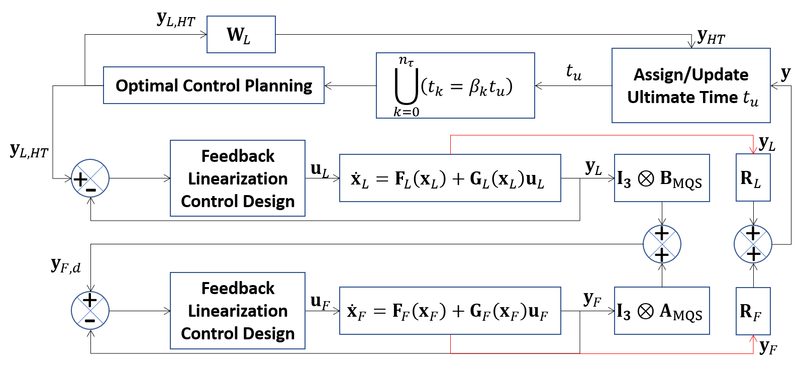
As shown in Fig. 2, $\mathbf{y}_{L,HT}(t)$ is the reference input of the control system of leader coordination, and

\mathbf{y}_{F,d}(t)=\left(\mathbf{I}_{3}\otimes\mathbf{A}_{\mathrm{MQS}}\right)\mathbf{y}_{F}(t)+\left(\mathbf{I}_{3}\otimes\mathbf{B}_{\mathrm{MQS}}\right)\mathbf{y}_{L}(t)

(82)

is the reference input of the control system of the follower quadcopter team.

V-B Trajectory Control Design

The objective of control design is to determine $\mathbf{u}_{L}\in\mathbb{R}^{12\times 1}$ and $\mathbf{u}_{F}$ such that (51) is satisfied at any time $t\in\left[t_{0},t_{u}\right]$ . We can rewrite the safety condition (51) as

\bigwedge_{i\in\mathcal{V}}\left(\left(\mathbf{y}(t)-\mathbf{y}_{HT}(t)\right)^{T}\mathbf{S}_{i}^{T}\mathbf{S}_{i}\left(\mathbf{y}(t)-\mathbf{y}_{HT}(t)\right)\leq\delta^{2}\right),\qquad\forall t,

(83)

where $\mathbf{S}_{i}=\left[\mathbf{S}_{i_{pq}}\right]\in\mathbb{R}^{3\times 3N}$ is defined as follows:

\mathbf{S}_{i_{pq}}=\begin{cases}1&\bigwedge_{i=1}^{3}\left(\left(p=i\right)\wedge\left(q=N(i-1)+i\right)\right)\\ 0&\mathrm{otherwise}\end{cases}.

(84)

We use the feedback linearization approach presented in Ref. [24] to obtain the control input vector $\mathbf{u}_{i}(t)$ for every quadcopter $i\in\mathcal{V}$ such that inequality constraint (83) is satisfied.

VI Simulation Results

We consider an MQS consisting of $N=8$ quadcopters with the initial formation shown in Fig. 3 (a). The MQS is initially distributed over horizontal plane $z=43m$ where $\bar{\mathbf{d}}_{s}=\begin{bmatrix}1935&215&43\end{bmatrix}^{T}$ is the position of the center of the containment ball $\mathcal{S}$ at the initial time $t_{s}=0s$ . It is desired that the MQS finally reaches the final formation shown in Fig. 3 (b) in an obstacle laden environment shown in Fig. 4. The final formation of the MQS is obtained by homogeneous transformation of the MQS initial formation and specified by choosing $\sigma_{1,n_{\tau}}=1.2$ , $\sigma_{2,n_{\tau}}={1\over\sigma_{1,n_{\tau}}}=0.83$ , $\theta_{d,n_{\tau}}=-{\pi\over 4}$ , and $\bar{\mathbf{d}}_{u}=\begin{bmatrix}850&2250&50\end{bmatrix}^{T}$ .

Inter-agent Communication: Given quadcopters’ initial positions, followers’ in-neighbors and communication weights are computed using the approach presented in Section V-A and listed in Table I. Note that quadcopters’ identification numbers are defined by set $\mathcal{V}=\{1,\cdots,10\}$ , where $\mathcal{V}_{L}=\{1,2,3\}$ and $\mathcal{V}_{F}=\{4,\cdots,10\}$ define the identification numbers of the leader and follower quadcopters, respectively.

Table I: In-neighbor agents of followers

4

through

33

and followers’ communication weights

	In-neighbors			Communication weights
$i\in\mathcal{V}_{F}$	$i_{1}$	$i_{2}$	$i_{3}$	$w_{i,i_{1}}$	$w_{i,i_{2}}$	$w_{i,i_{3}}$
4	1	7	8	0.55	0.15	0.30
5	2	6	8	0.60	0.15	0.25
6	3	5	7	0.60	0.15	0.25
7	4	6	8	0.40	0.20	0.40
8	4	5	7	0.45	0.25	0.30

Safety Specification: We assume that every quacopter can be enclosed by a ball of radius $\epsilon=0.45m$ . For the initial formation shown in Fig. 3 (a), $d_{\mathrm{min}}=3.5652m$ is the minimum separation distance between every two quadcopters. Furthermore, $\sigma_{\mathrm{min}}={1\over\sigma_{1,n_{\tau}}}=0.83$ is the lower bound for the eigenvalues of matrix $\mathbf{U}_{xy}$ . Per Eq. (54),

\delta={1\over 2}\left(d_{\mathrm{min}}\sigma_{\mathrm{min}}-2\epsilon\right)=1.04m

is the upper-bound for deviation of every quadcopter from its global desired position at any time $t\in\left[t_{0},t_{u}\right]$ .

MQS Planning: It is desired that the MQS remains inside a ball of radius $r_{\mathrm{max}}=50m$ at any time $t\in[t_{0},t_{u}]$ . By using A* search method, the optimal intermediate waypoints of the center of the containment ball are obtained. Then, the optimal path of the containment ball is assigned and shown in Fig. 4. Given the intermediate waypoints of the center of containment ball, the desired trajectories of the leaders are determined by solving the constrained optimal control problem given in Section IV-C. Given $t_{s}=0s$ and $\delta=1.04m$ , $t_{u}=490s$ is assigned by using Algorithm 3. Components of the optimal control input vector $\mathbf{u}_{L}^{*}(t)$ , $\ddot{x}_{1,HT}^{*}(t)$ , $\ddot{x}_{2,HT}^{*}(t)$ , $\ddot{x}_{3,HT}^{*}(t)$ , $\ddot{y}_{1,HT}^{*}(t)$ , $\ddot{y}_{2,HT}^{*}(t)$ , and $\ddot{y}_{3,HT}^{*}(t)$ , and components of global desired positions of leaders, ${x}_{1,HT}^{*}(t)$ , ${x}_{2,HT}^{*}(t)$ , ${x}_{3,HT}^{*}(t)$ , ${y}_{1,HT}^{*}(t)$ , ${y}_{2,HT}^{*}(t)$ , and ${y}_{3,HT}^{*}(t)$ , are plotted versus time $t$ in Figs. 5 and 6, respectively. Furthermore, deviation of every quadcopter from the global desired position is plotted in Fig. 7. It is seen that deviation of no quadcopter exceeds $\delta=1.04m$ at any time $t\in[0,490]s$ .

VII Conclusion

This paper developed an algorithmic and formal approach for continuum deformation planning of a multi-quadcopter system coordinating in a geometrically-constrained environment. By using the principles of Lagrangian continuum mechanics, we obtained safety conditions for inter-agent collision avoidance and follower containment through constraining the eigenvalues of the Jacobian matrix of the continuum deformation coordination. To obtain safe and optimal transport of the MQS, we contain the MQS by a rigid ball, and determine the intermediate waypoints of the containment ball using the A* search method. Given the intermediate configuration of the containment ball, we first determined the leaders’ intermediate configurations by decomposing the homogeneous deformation coordination. Then, we assigned the optimal desired trajectories of the leader quadcopters by solving a constrained optimal control problem.

VIII Acknowledgement

This work has been supported by the National Science Foundation under Award Nos. 1914581 and 1739525. The author gratefully thanks Professor Ella Atkins.

References

[1] J. Zhang, J. Yan, P. Zhang, and X. Kong, “Collision avoidance in fixed-wing uav formation flight based on a consensus control algorithm,” IEEE Access, vol. 6, pp. 43 672–43 682, 2018.
[2] S.-L. Du, X.-M. Sun, M. Cao, and W. Wang, “Pursuing an evader through cooperative relaying in multi-agent surveillance networks,” Automatica, vol. 83, pp. 155–161, 2017.
[3] A. Artuñedo, R. M. Del Toro, and R. E. Haber, “Consensus-based cooperative control based on pollution sensing and traffic information for urban traffic networks,” Sensors, vol. 17, no. 5, p. 953, 2017.
[4] B. Cheng, X. Wang, and Z. Li, “Event-triggered consensus of homogeneous and heterogeneous multiagent systems with jointly connected switching topologies,” IEEE transactions on cybernetics, vol. 49, no. 12, pp. 4421–4430, 2018.
[5] Z. Tu, H. Yu, and X. Xia, “Decentralized finite-time adaptive consensus of multiagent systems with fixed and switching network topologies,” Neurocomputing, vol. 219, pp. 59–67, 2017.
[6] F. Muñoz, E. S. Espinoza Quesada, H. M. La, S. Salazar, S. Commuri, and L. R. Garcia Carrillo, “Adaptive consensus algorithms for real-time operation of multi-agent systems affected by switching network events,” International Journal of Robust and Nonlinear Control, vol. 27, no. 9, pp. 1566–1588, 2017.
[7] T. Liu and J. Huang, “Leader-following attitude consensus of multiple rigid body systems subject to jointly connected switching networks,” Automatica, vol. 92, pp. 63–71, 2018.
[8] Q. Ma and S. Xu, “Consensus switching of second-order multiagent systems with time delay,” IEEE Transactions on Cybernetics, 2020.
[9] X. Wang and G.-H. Yang, “Fault-tolerant consensus tracking control for linear multiagent systems under switching directed network,” IEEE transactions on cybernetics, vol. 50, no. 5, pp. 1921–1930, 2019.
[10] M. A. Shahab, B. Mozafari, S. Soleymani, N. M. Dehkordi, H. M. Shourkaei, and J. M. Guerrero, “Distributed consensus-based fault tolerant control of islanded microgrids,” IEEE Transactions on Smart Grid, vol. 11, no. 1, pp. 37–47, 2019.
[11] Q. Liu, Z. Wang, X. He, and D. Zhou, “On kalman-consensus filtering with random link failures over sensor networks,” IEEE Transactions on Automatic Control, vol. 63, no. 8, pp. 2701–2708, 2017.
[12] H. J. LeBlanc and X. D. Koutsoukos, “Consensus in networked multi-agent systems with adversaries,” in Proceedings of the 14th international conference on Hybrid systems: computation and control, 2011, pp. 281–290.
[13] M. Ji, G. Ferrari-Trecate, M. Egerstedt, and A. Buffa, “Containment control in mobile networks,” IEEE Transactions on Automatic Control, vol. 53, no. 8, pp. 1972–1975, 2008.
[14] H. Liu, G. Xie, and L. Wang, “Necessary and sufficient conditions for containment control of networked multi-agent systems,” Automatica, vol. 48, no. 7, pp. 1415–1422, 2012.
[15] B. Li, Z.-q. Chen, Z.-x. Liu, C.-y. Zhang, and Q. Zhang, “Containment control of multi-agent systems with fixed time-delays in fixed directed networks,” Neurocomputing, vol. 173, pp. 2069–2075, 2016.
[16] H. Su and M. Z. Chen, “Multi-agent containment control with input saturation on switching topologies,” IET Control Theory & Applications, vol. 9, no. 3, pp. 399–409, 2015.
[17] M. Asgari and H. Atrianfar, “Necessary and sufficient conditions for containment control of heterogeneous linear multi-agent systems with fixed time delay,” IET Control Theory & Applications, vol. 13, no. 13, pp. 2065–2074, 2019.
[18] H. Atrianfar, “Sampled-time containment control of high-order continuous-time mass under heterogenuous time-varying delays and switching topologies: a scrambling matrix approach,” Neurocomputing, vol. 395, pp. 24–38, 2020.
[19] G. Cui, S. Xu, Q. Ma, Z. Li, and Y. Chu, “Command-filter-based distributed containment control of nonlinear multi-agent systems with actuator failures,” International Journal of Control, vol. 91, no. 7, pp. 1708–1719, 2018.
[20] D. Ye, M. Chen, and K. Li, “Observer-based distributed adaptive fault-tolerant containment control of multi-agent systems with general linear dynamics,” ISA transactions, vol. 71, pp. 32–39, 2017.
[21] S. Zuo, F. L. Lewis, and A. Davoudi, “Resilient output containment of heterogeneous cooperative and adversarial multigroup systems,” IEEE Transactions on Automatic Control, vol. 65, no. 7, pp. 3104–3111, 2019.
[22] H. Qin, H. Chen, Y. Sun, and L. Chen, “Distributed finite-time fault-tolerant containment control for multiple ocean bottom flying node systems with error constraints,” Ocean Engineering, vol. 189, p. 106341, 2019.
[23] T. Xu, G. Lv, Z. Duan, Z. Sun, and J. Yu, “Distributed fixed-time triggering-based containment control for networked nonlinear agents under directed graphs,” IEEE Transactions on Circuits and Systems I: Regular Papers, vol. 67, no. 10, pp. 3541–3552, 2020.
[24] H. Rastgoftar, E. M. Atkins, and I. Kolmanovsky, “Scalable vehicle team continuum deformation coordination with eigen decomposition,” arXiv preprint arXiv:2002.03036, 2020.
[25] H. Rastgoftar, “Fault-resilient continuum deformation coordination,” IEEE Transactions on Control of Network Systems, 2020.