Chandra Observations of the Planck ESZ Sample: A Re-Examination of Masses and Mass Proxies
Abstract
Using Chandra observations, we derive the proxy and associated total mass measurement, , for 147 clusters with from the Planck Early Sunyaev-Zel’dovich catalog, and for 80 clusters with from an X-ray flux-limited sample. We re-extract the Planck measurements and obtain the corresponding mass proxy, , from the full Planck mission maps, minimizing the Malmquist bias due to observational scatter. The masses re-extracted using the more precise X-ray position and characteristic size agree with the published PSZ2 values, but yield a significant reduction in the scatter (by a factor of two) in the – relation. The slope is , and the median ratio, , is within the expectations from known X-ray calibration systematics. The ratio is , in good agreement with predictions from cluster structure, and implying a low level of clumpiness. In agreement with the findings of the Planck Collaboration, the slope of the – flux relation is significantly less than unity (). Using extensive simulations, we show that this result is not due to selection effects, intrinsic scatter, or covariance between quantities. We demonstrate analytically that changing the – relation from apparent flux to intrinsic properties results in a best-fit slope that is closer to unity and increases the dispersion about the relation. The redistribution resulting from this transformation implies that the best fit parameters of the – relation will be sample-dependent.
Keywords:
galaxy clusters: general — cosmology: large-structure of universeI Introduction
Galaxy clusters reside in the highest ranges of the halo mass function. In the standard CDM cosmology, massive halos form by the accretion of smaller sub-clumps (Jones et al. 1979; Forman & Jones 1982; Allen et al. 2011; Kravtsov & Borgani 2012, e.g.,). Under the influence of gravity, uncollapsed and collapsed sub-clumps fall into larger halos and, occasionally, objects of comparable mass merge with one another. X-ray observations of substructures in galaxy clusters (Jones & Forman 1984; Jones & Forman 1999; Mohr et al. 1995; Buote & Tsai 1996; Jeltema et al. 2005; Böhringer et al. 2010; Laganá et al. 2010; Andrade-Santos et al. 2012; Andrade-Santos et al. 2013, see, for instance,) and measurements of the growth of structure (Vikhlinin et al. 2009b; Mantz et al. 2010; Allen et al. 2011; Benson et al. 2013; Planck Collaboration XX 2014; Planck Collaboration XXIV 2016) show that these objects are still in the process of formation.
A well established relation between the cluster mass and its observables (such as X-ray luminosity, gas temperature, etc) is crucial to any work that explores the theoretical relation between the number density of collapsed halos (the mass function) and the underlying cosmological parameters (Vikhlinin et al. 2009b; Planck Collaboration XX 2014; Planck Collaboration XXIV 2016; Pratt et al. 2019). The relations between a cluster’s observables and its mass are a direct consequence of gravity, which is the main force driving cluster evolution (Kaiser 1986). Departures from the purely gravitational self-similar expectation are usually attributed to non-gravitational processes, such as radiative cooling, AGN feedback, etc. (Voit et al. 2005; Pratt et al. 2010, e.g.).

The Planck satellite surveyed the entire sky across nine microwave frequency bands. The resulting data set allowed the detection of galaxy clusters through the thermal Sunyaev-Zel’dovich (SZ) effect (Sunyaev & Zeldovich 1972). The thermal SZ effect is the shift of the CMB spectrum towards higher frequencies caused by the inverse Compton scattering of the CMB photons by the hot electrons in the ICM. Being proportional to the line-of-sight integral of the ICM pressure, the SZ signal is expected to be closely related to the cluster total mass (da Silva et al. 2004; Pike et al. 2014, e.g.), and the amplitude of its signal is independent of the cluster redshift, since the CMB photons were all emitted at a constant redshift of . As a consequence, SZ surveys can potentially build unbiased cluster samples, covering higher redshifts than X-ray samples, and are expected to be close to mass-limited.
The second Planck catalogue (Planck Collaboration XXVII 2016, PSZ2,), derived from the full High Frequency Instrument (HFI) survey of 29 months, detected 1653 cluster candidates. The vast majority ( 1200) of these candidates have been confirmed, making the PSZ2 catalog a reference for cluster studies. Among the many quantities provided by the PSZ2 catalog for each cluster, the mass estimate is arguably the most important. Since the Planck masses were determined using XMM-Newton data to calibrate the – relation, comparing Chandra X-ray derived masses to SZ derived masses provides an independent and invaluable test for the Planck mass estimates.
Here we use Chandra observations to compute the masses for 147 Planck ESZ clusters at . All of the clusters have Planck SZ masses, and we compare these to the X-ray derived masses from our Chandra analysis. We compare the results with those obtained from observations of an X-ray selected sample of the 80 of the 100 highest flux X-ray clusters at Galactic latitudes and . We also study the – relation. Our aim is to examine the – relation and to compare X-ray and SZ masses for these clusters. We use the SZ-selected clusters as our baseline sample, and the X-ray-selected objects only for comparison. Examination of the impact of our findings on the Planck SZ cosmological constraints is beyond the scope of the present work.
Throughout this paper, we assume a standard CDM cosmology with , , and . The variables and are the total mass within and radius corresponding to a total density contrast as compared to , the critical density of the universe at the cluster redshift. The SZ flux is characterised by (in arcmin2), or simply . The quantity is then the spherically integrated Compton parameter within (in Mpc2), where is the angular-diameter distance of the cluster. All uncertainties are quoted at the (68% confidence) level. The natural logarithm is denoted ln, while log denotes the decimal logarithm.

II SZ and X-ray selected clusters
For our investigation, we make use of the following cluster samples:
- •
An SZ-selected sample of clusters derived from the first catalog of 189 objects detected in the first 10 months of the Planck survey, and released in early 2011 (Planck Collaboration VIII 2011). A Chandra XVP (X-ray Visionary Program – PI: Jones) and HRC Guaranteed Time Observations (PI: Murray) were combined to form the Chandra-Planck Legacy Program for Massive Clusters of Galaxies. For each of the 163 ESZ Planck clusters at , we obtained Chandra exposures sufficient to collect at least 10,000 source counts11 1 hea-www.cfa.harvard.edu/CHANDRA_PLANCK_CLUSTERS/.
The second Planck catalogue (Planck Collaboration XXVII 2016, PSZ2,), derived from the full mission maps, provided masses for 157 of the original set of 163 ESZ clusters at . The remaining six clusters are not in the PSZ2 catalog, simply because they fall outside the mask used to construct that catalog (i.e. they are close to point sources). We can thus discard those without changing the sample selection function. We use the PSZ2 mass estimates of the resulting systems as they are largely independent of the original detection (discussed in more detail below). Of the resulting 157 clusters, nine are classed as multiple, defined as having more than one object (visually identified in the X-ray images) at a distance less than 10’ from the main system. These were removed from the following as the presence of more than one system may lead to a boosting of the SZ signal due to confusion in the Planck beam. We also discarded the very nearby cluster PLCKESZ G234.59+73.01 (A 1367 at ) as it is too large to allow a reliable background estimate in the Chandra pointing. Figure 1 displays a mosaic of the 147 clusters from the ESZ sample that were used in this work.
- •
An X-ray selected sample of high-flux clusters. Voevodkin & Vikhlinin 2004 compiled a sample of the 52 X-ray brightest clusters in the local universe by selecting the highest flux objects detected in the ROSAT All-Sky survey at and -- using the HIFLUGCS22 2 HIFLUGCS – The HIghest X-ray FLUx Galaxy Cluster Sample (Reiprich & Böhringer 2002; Schellenberger & Reiprich 2017) catalog as reference. The sample used here is an extension of Voevodkin & Vikhlinin 2004’s approach, where the flux limit in the 0.5 – 2.0 keV band was lowered to . The full sample contains 100 clusters; the highest-redshift object is at . All have Chandra observations.
Eighty-three of the clusters from this sample have Planck SZ masses. Three of these were classified as multiple, according to the definition applied to the ESZ sample, so after removing these clusters we obtained a sample of 80 clusters. Of these, 45 are also in the ESZ sample, and 42 are in the HIFLUGCS sample. Figure 2 displays a mosaic of the 80 clusters from the X-ray sample that were used in this work.
The left panel of Figure 3 presents the redshift distribution of both cluster samples. The Planck detected clusters are clearly more broadly distributed in redshift than the X-ray clusters. This is due to the nature of the selection: for resolved clusters the Sunyaev-Zel’dovich signal is independent of the redshift of the cluster because it is the CMB that is distorted (the CMB photons originate at the epoch of recombination – from a constant redshift of ), while the X-ray selected clusters constitute a flux-limited sample, which strongly favors the X-ray brighter, lower redshift clusters. The right panel of Figure 3 presents the mass (derived using the proxy) distribution of both samples, showing that the X-ray sample has on average lower mass than the Planck ESZ sample.
III Data Reduction
III.1 Chandra data
III.1.1 Event file processing
Our Chandra data reduction followed the process described in Vikhlinin et al. 2005. We applied the calibration files CALDB 4.7.2. The data reduction included corrections for the time dependence of the charge transfer inefficiency and gain, and also a check for periods of high background, which were then omitted. Standard blank sky background files and readout artifacts were subtracted. We also detected compact X-ray sources in the 0.7–2.0 keV and 2.0–7.0 keV bands using CIAO’s wavdetect and then masked these sources, as well as extended substructures, before performing the spectral and spatial analyses of the cluster emission. For each cluster, we used all available Chandra ACIS (ACIS-I and ACIS-S) observations within 2 Mpc from the cluster center. The median maximum radius of the observations is (with a maximum radius greater than for of the sample) and the median azimuthal coverage is . We have checked that our results do not depend either on the maximum radius or on the coverage.
III.1.2 Emission measure profiles
We refer to Vikhlinin et al. 2006 for a detailed description of the procedures we used to compute the emission measure profile for each cluster. We outline here only the main aspects of the method.
We measured the surface brightness profiles in the 0.7–2.0 keV energy band, which maximizes the signal to noise ratio in Chandra observations for typical cluster gas temperatures. We used the X-ray peak as the cluster center. The readout artifacts and blank-field background (Vikhlinin et al. 2006, see section 2.3.3 of) were subtracted from the X-ray images, and the results were then exposure-corrected, using exposure maps computed assuming an absorbed optically-thin thermal plasma with keV, abundance = 0.3 solar, with the Galactic column density and including corrections for bad pixels and CCD gaps, which do not take into account spatial variations of the effective area. We subtracted a small uniform component, corresponding to soft X-ray foreground adjustments, if required (determined by fitting a thermal model in a region of the detector field most distant from the cluster center, properly taking into account the expected thermal contribution from the cluster).
Following these steps, we extracted the surface brightness in narrow concentric annuli () centered on the X-ray peak and computed the Chandra area-averaged effective area for each annulus (see Vikhlinin et al. 2005, for details on calculating the effective area). To compute the emission measure and temperature profiles, we assumed spherical symmetry. The spherical assumption is expected to introduce only small deviations in the emission measure profile (Piffaretti et al. 2003). Using the modeled de-projected temperature (Andrade-Santos et al. 2017, see), effective area, and metallicity as a function of radius, we converted the Chandra count rate in the 0.7–2.0 keV band into the emission integral, , within each cylindrical shell. Online tables in machine-readable format list the maximum cluster radius where the emission integral is computed () for each cluster. 142 () clusters in the ESZ sample have 33 3 defines the radius at the over-density of 500 times the critical density of the Universe at the cluster redshift. This quantity was obtained from the X-ray derived masses., and in the X-ray sample, 72 () clusters satisfy this condition (four of the eight clusters that do not satisfy this condition are also in the ESZ sample). We have an average azimuthal coverage within of for the ESZ clusters and for the X-ray clusters.

We fit the emission measure profile assuming the gas density profile follows that given by Vikhlinin et al. 2006:
| (1) | |||||
where the parameters and determine the normalizations of both additive components. , , , and are indices controlling the slope of the curve at characteristic radii given by the parameters , , and . controls the width of the transition region given by . Although the relation given by Equation 1 is based on a classic -model (Cavaliere & Fusco-Femiano 1976), it is modified to account for a central power-law type cusp and a steeper emission measure slope at large radii. In addition, a second -model is included, to better characterize the cluster core. For further details on this equation, we refer the reader to Vikhlinin et al. 2006. In the fit to the emissivity profile, all parameters are free to vary. For a typical metallicity of 0.3 , the reference values from Anders & Grevesse 1989 yield . Examples of projected emissivity and gas density profiles are presented in Figure 4.
III.1.3 Cluster Mass Estimates
Using the gas mass and temperature, we estimated the total cluster mass from the – scaling relation of Vikhlinin et al. 2009a,
| (2) |
where , is computed using the best fit parameters of Equation (1), and is the measured temperature in the (0.15–1) range. We fit the spectrum in the 0.7–7.0 keV energy range with an absorbed APEC model, fixing NH to the total Galactic value (Willingale et al. 2013, molecular plus atomic hydrogen contributions –). The parameters , and (Vikhlinin et al. 2009a). Here, is the total mass within , and is the function describing the evolution of the Hubble parameter with redshift. Using Equation (2), is computed by solving
| (3) |
where is the critical density of the Universe at the cluster redshift. In practice, Equation (2) is evaluated at a given radius, whose result is compared to the evaluation of Equation (3) at the same radius. This process is repeated in an iterative procedure, until the fractional mass difference is less than 1%. We estimated 1 statistic uncertainties in the derived masses using Monte Carlo simulations. We also added to the Monte Carlo procedure a 1 systematic uncertainty of 9% in the mass determination, as discussed by Vikhlinin et al. 2009a.
III.2 Planck data
III.2.1 Published masses
Derivation of the published Planck masses is extensively described in Planck Collaboration XXVII 2016. The mass was estimated from the relation between and (Planck Collaboration XX 2014):
| (4) |
The SZ size-flux degeneracy was broken through the use of the scaling relation linking the SZ flux to the angular size, , that is then intersected with the two-dimensional posterior probability contours in the ) plane. For the PSZ2 masses, , the – prior was obtained from the intrinsic relation between and for a given redshift :
| (5) |
where .
We recall that Equation (4) was calibrated on a baseline mass proxy relation linking the hydrostatic mass and the X-ray analog of the SZ Compton parameter, . As described in Planck Collaboration XXVII 2016, the resulting SZ mass can be viewed as the hydrostatic mass expected for a cluster consistent with the assumed scaling relation, at a given redshift, and given the measured ) posterior information. Hereafter we will refer to and simply as and .
III.2.2 Re-extracted masses
As discussed in Appendix A of Planck Collaboration XI 2011, a refined measurement of the SZ flux can be obtained by using higher-quality prior information on the position and size of the cluster. Such information is readily provided by our Chandra observations. In the following, we refer to the re-extracted masses as . The SZ signal was thus re-extracted from the six HFI temperature channel maps corresponding to the full Planck mission survey. We used full resolution maps of HEALPix (Górski et al. 2005)44 4 http://healpix.jpl.nasa.gov and assumed that the beams were described by circular Gaussians. We adopted beam FWHM values of 9.66, 7.22, 4.90, 4.92, 4.68, and 4.22 arcmin for channel frequencies 100, 143, 217, 353, 545, and 857 GHz, respectively. Bandpass uncertainties were taken into account in the flux measurement. Uncertainties due to beam corrections and map calibrations are expected to be small, as discussed extensively in Planck Collaboration VIII 2011, Planck Collaboration IX 2011, Planck Collaboration X 2011 and Planck Collaboration XI 2011.
| Cluster | RA | DEC | ||||||||
|---|---|---|---|---|---|---|---|---|---|---|
| () | () | () | () | () | () | () | ||||
| G000.44-41.83 | 21:04:18.603 | -41:20:39.36 | 0.165 | 4.81 | 0.47 | 4.89 | 0.32 | 5.30 | 0.33 | 1.68 |
| G002.74-56.18 | 22:18:39.822 | -38:53:58.47 | 0.141 | 5.34 | 0.51 | 4.24 | 0.30 | 4.41 | 0.30 | 1.55 |
| G003.90-59.41 | 22:34:27.334 | -37:44:07.88 | 0.151 | 9.23 | 0.89 | 7.26 | 0.24 | 7.19 | 0.26 | 1.37 |
| G006.47+50.54 | 15:10:56.117 | 05:44:40.38 | 0.077 | 7.06 | 0.64 | 7.19 | 0.17 | 7.04 | 0.20 | 1.43 |
| G006.70-35.54 | 20:34:46.912 | -35:49:24.54 | 0.089 | 5.22 | 0.50 | 4.40 | 0.21 | 4.17 | 0.23 | 1.66 |
| G006.78+30.46 | 16:15:46.073 | -06:08:54.61 | 0.203 | 17.53 | 2.01 | 16.25 | 0.26 | 16.12 | 0.29 | 1.08 |
| G008.30-64.75 | 22:58:48.095 | -34:48:04.62 | 0.312 | 7.97 | 0.75 | 7.70 | 0.40 | 7.75 | 0.40 | 1.50 |
| G008.44-56.35 | 22:17:45.701 | -35:43:32.55 | 0.149 | 3.84 | 0.39 | 4.41 | 0.27 | 4.79 | 0.30 | 1.82 |
| G008.93-81.23 | 00:14:19.305 | -30:23:29.33 | 0.307 | 10.22 | 0.93 | 9.23 | 0.36 | 9.84 | 0.39 | 1.37 |
| G018.53-25.72 | 20:03:30.848 | -23:23:37.54 | 0.317 | 9.79 | 0.93 | 8.65 | 0.45 | 8.99 | 0.47 | 1.42 |
Note. — Columns list cluster name (ESZ Planck cluster name with the prefix PLCKESZ omitted), right ascension, declination, redshift, derived Chandra mass, derived Chandra mass uncertainty, PSX Planck mass, PSX Planck mass uncertainty, PSZ2 Planck mass, PSZ2 Planck mass uncertainty, and maximum cluster radius where the emission integral is computed in terms of ( was computed using the derived Chandra mass).
| Cluster | RA | DEC | ||||||||
|---|---|---|---|---|---|---|---|---|---|---|
| () | () | () | () | () | () | () | ||||
| G006.47+50.54 | 15:10:56.117 | 05:44:40.38 | 0.077 | 7.06 | 0.64 | 7.19 | 0.17 | 7.04 | 0.20 | 1.43 |
| G006.70-35.54 | 20:34:46.912 | -35:49:24.54 | 0.089 | 5.22 | 0.50 | 4.40 | 0.21 | 4.17 | 0.23 | 1.66 |
| G006.78+30.46 | 16:15:46.073 | -06:08:54.61 | 0.203 | 17.53 | 2.01 | 16.25 | 0.26 | 16.12 | 0.29 | 1.08 |
| G021.09+33.25 | 16:32:46.854 | 05:34:31.61 | 0.151 | 8.47 | 0.77 | 8.07 | 0.27 | 7.79 | 0.30 | 1.42 |
| G029.00+44.56 | 16:02:14.068 | 15:58:16.23 | 0.035 | 2.86 | 0.26 | 2.64 | 0.13 | 3.53 | 0.06 | 1.01 |
| G033.78+77.16 | 13:48:52.710 | 26:35:31.20 | 0.062 | 5.67 | 0.51 | 4.72 | 0.14 | 4.47 | 0.14 | 1.53 |
| G042.82+56.61 | 15:22:29.473 | 27:42:18.76 | 0.072 | 5.63 | 0.51 | 4.44 | 0.20 | 4.08 | 0.19 | 1.47 |
| G044.22+48.68 | 15:58:21.100 | 27:13:47.87 | 0.089 | 12.36 | 1.12 | 9.44 | 0.18 | 8.77 | 0.20 | 1.25 |
| G046.50-49.43 | 22:10:19.489 | -12:10:10.03 | 0.085 | 5.09 | 0.48 | 4.51 | 0.20 | 4.39 | 0.20 | 1.60 |
| G048.05+57.17 | 15:21:12.694 | 30:38:00.59 | 0.078 | 3.92 | 0.36 | 3.66 | 0.23 | 3.59 | 0.21 | 1.77 |
Note. — Same as Table 1, except for the X-ray sample.
We extracted the SZ signal using multi-frequency matched filters (Herranz et al. 2002; Melin et al. 2006, MMF,). These require information on the instrumental beam, the SZ frequency spectrum, and a cluster profile; noise auto- and cross-spectra are estimated directly from the data. We used the MMF in a targeted mode, extracting the SZ flux from a position centered on the X-ray emission peak using the “universal” pressure profile of Arnaud et al. 2010 as a spatial template, in an aperture corresponding to the determined in Sect. III.1.3 above. The extraction was achieved by excising a patch with pixel size , centered on the X-ray position, from the six HFI maps, and estimating the SZ flux using the MMF. The profiles were truncated at to ensure integration of the total SZ signal. The flux and corresponding error were then scaled to using the profile assumed for extraction, yielding the refined estimate of . The resulting refined mass estimate PSX was calculated as described above, using the – relation and the measured ) posterior information.
III.3 Fitting Procedure
We fit each scaling relation between a pair of observables with a power law of the form
| (6) |
assuming no evolution, as expected in the self-similar model. The reason for the latter decision is that the redshift leverage is insufficient to put a strong constraint on the evolution because the maximum redshift of the sample is . Figure 5 shows that the data are indeed consistent with no evolution in the current sample. The pivot points were , Mpc2, and arcmin2 for , , and respectively.
The fit was undertaken using linear regression in the log–log plane, taking the uncertainties in both variables into account and intrinsic scatter. The X-ray and SZ measurements are independent, so there is no covariance between statistical errors for the scaling laws studied here.
We used the orthogonal Bivariate Correlated Errors and intrinsic Scatter (Akritas & Bershady 1996, BCES) linear regression method to perform the baseline fits. BCES is widely used by the astronomical community, giving results that may easily be compared with other data sets fitted using the same method. The intrinsic vertical scatter was computed from the quadratic difference between the raw scatter and that expected from the statistical uncertainties, as described in Pratt et al. 2009 and Planck Collaboration XI 2011.
We also fit the data using a Bayesian maximum likelihood estimation approach, with Markov Chain Monte Carlo (MCMC) sampling. Using the emcee package developed by Foreman-Mackey et al. 2013, we write the likelihood as described by Robotham & Obreschkow 2015.
| (7) | |||||
| (8) |
with the intrinsic scatter, , as a free parameter. We used flat priors on the parameters, with ranges , , and , for , , and , respectively. For comparison, we also used the LINMIX (Kelly 2007) and LIRA (Sereno 2016) Bayesian regression packages, with default priors. The latter, as well as LINMIX, allows to correct for the Eddington bias due to the non-uniform distribution of the covariate in the presence of intrinsic scatter (Sereno & Ettori 2015; Sereno 2016). For LIRA, we used the option sigma.XIZ.0=‘prec.dgamma’ and a single Gaussian component for the corresponding latent variable (we checked that adding an additional component does not change the results). For LINMIX, we use the default setting of three gaussians.
The fit results are detailed in Table 3, where it can be seen that the differences in slope and normalization between methods are always less than the statistical error on the parameters. We also note the excellent agreement between LIRA and BCES, suggesting that the Eddington bias due to the non-uniform distribution in the X variable is not an issue.
Table 3 also gives the mean ratio between SZ and X-ray quantities. This was computed by maximizing the likelihood of the logarithm of the ratios in log-log space, taking into account the statistical errors and an intrinsic scatter. We also computed the ratio by weighting each value of the logarithm ratio by the quadratic sum of the statistical error and the intrinsic scatter. This scatter and the weighted mean were then estimated simultaneously by iteration. Both methods give consistent results.
In Planck Collaboration XXIX 2014, the – relation for the PSZ1 catalog was corrected for the Malmquist bias affecting the determination (see their Figure 32). The correction was made on a cluster-by-cluster basis, following the approach proposed by Vikhlinin et al. 2009a. The clusters in our study are from the ESZ catalog, which were detected in the Planck maps corresponding to the first 10 months of the survey. However, here we use the SZ signal from the PSZ2 catalog, re-extracted from the full mission maps. Although the maps are not fully independent, they correspond to significantly different noise realizations and we thus expect the re-extracted SZ signal from the PSZ2 maps to be much less affected by Malmquist bias than the original ESZ detection signal. As a first approximation, in the following we assume that the SZ signal is independent of the detection and neglect residual selection effects from Malmquist bias. We discuss the impact of this assumption extensively in Sect. V.1 and Appendix A.
| Relation | |||
|---|---|---|---|
| BCES orthogonal | |||
| – | |||
| – | – | ||
| – | |||
| – | |||
| LINMIX | |||
| – | |||
| – | |||
| – | |||
| – | |||
| MCMC | |||
| – | |||
| – | – | ||
| – | |||
| – | |||
| LIRA | |||
| – | |||
| – | |||
| – | |||
| – | |||
| Ratio | Mean value | ||
IV Results
IV.1 The – relation
The total cylindrical Sunyaev-Zel’dovich signal is given by the integral of the Compton parameter, , where is the solid angle, and the Compton parameter is given by:
| (9) |
where is the Thomson cross section, is the electron rest mass energy, is the distance along the line of sight, and is the Boltzmann constant. The total Sunyaev-Zel’dovich signal within can also be expressed as (in its spherical form)55 5 The Planck Collaboration performed the Compton integral within a sphere, instead of performing it along the line of sight to infinity (cylindrical integral). :
| (10) |
where is the angular size distance of the cluster and is the sphere of radius .
The X-ray analog of the Sunyaev-Zel’dovich Compton parameter is defined as , where is the gas mass given by:
| (11) |
where is the mean molecular weight per electron, is the proton mass, and is the X-ray measured temperature in the (0.15–1.0) radial range.
On the other hand, the mass-weighted temperature is given by:
| (12) |
which, when combined with Equations 9 and 11, results in:
| (13) |
where is given by:
| (14) |
where we used , which was calculated assuming a fully ionized plasma with metallicity of 0.3 , and reference values from Anders & Grevesse 1989.
In practice, when computing , we used the fact that the emission measure is proportional to , averaged in radial annuli, to estimate . For a uniform spherical gas distribution, , so one can recover the gas density. However, the reality is different, with typically . Defining the clumping factor as , we have . By definition , so we can write:
| (15) |
The – relation is thus a fundamental probe of the consistency of the SZ and X-ray signal. When extracted within the same aperture (here Chandra ), the ratio does not depend on any mass calibration. It depends on clumpiness, internal structure (mass weighted temperature versus spectroscopic temperature), and absolute calibration of X-ray measured temperature (Adam et al. 2017, see e.g. the discussion in). The – relation is expected to have a slope of one (if clusters are self-similar in shape), and a normalization less than one due to the radial dependence of the temperature. In the following, will refer to the quantity renormalised by the factor (Eq. 14), ie. expressed in units of Mpc2.
The left-hand panel of Figure 6 shows the the – relation, i.e. the correlation between the cluster physical properties – the intrinsic Compton parameter and . The slope, , is consistent with unity at slightly more than one sigma, while the normalization is . The slope of the relation is consistent with that found by Planck Collaboration XXIX 2014, displayed in Figure 6 by the orange line, within the statistical errors. The relation found by Rozo et al. 2012 using Chandra data, shown in green in Figure 6, has a somewhat shallower slope.
However, the picture changes when the – relation is plotted, i.e. when considering the observed SZ flux (arcmin2). When plotted this way, the slope is clearly not consistent with unity, . The effect is similar to, and in agreement with, that observed in Planck Collaboration XXIX 2014, , although at higher statistical precision (see their Section 7 and Appendix D).
IV.2 Comparison between SZ and X-ray derived masses
We next investigated the relation between the published Planck masses, , and those obtained from the Chandra data via the – relation, , as described above in Section III.1.3. The left-hand panel of Figure 7 compares the published Planck PSZ2 masses to those from Chandra for the 147 ESZ objects. The slope of the relation, , is less than unity at slightly more than the level. This translates into an ratio that decreases from to between and .
The right-hand panel of Figure 7 shows the SZ mass re-extracted at the X-ray position and size, , compared to the Chandra values. The main effect is a decrease of the intrinsic scatter by about a factor of two (from 11% to 6%). The slope, is unchanged, although the uncertainty is smaller as a result of the decreased scatter. As the X-ray mass is slightly higher than the PSZ2 mass, fixing the size to the X-ray value tends to increase the SZ mass on average, while extracting the SZ signal at the X-ray position has the opposite effect (the blind SZ signal is extracted at the position maximising the signal-to-noise). As a result the median SZ to X-ray mass ratio, , is unchanged, within the statistical errors.
In the following, we use the value as reference, as it is directly physically related to the quantity, and we will refer to it as .
IV.3 X-ray selected clusters
Here we consider the effect of adding the X-ray selected clusters to the relations discussed above. These clusters are discussed only for comparison to the SZ-selected objects.
The top-left panel of Figure 8 shows the – relation for the X-ray selected clusters only. It can be seen that these objects clearly populate the low mass part of the plot, with the majority of the systems having . The effect of adding the SZ selected clusters, as shown in the right-hand panel of Figure 8, is to transform what was a relation with a slope slightly less than unity (i.e. the SZ selected clusters only) into one with a clear offset in normalization. For the full sample of SZ + X-ray selected clusters, the slope , and the median ratio .
To shed light on the above, we can use the corresponding intrinsic – relation, which is shown in the bottom-left hand panel of Figure 8. We observe that as expected, the SZ and X-ray selected objects are distributed in the – plane in a similar fashion to their distribution in the – plane: the X-ray selected clusters tend to have higher values for a given .
The bottom-right hand panel of Figure 8 shows the - relation expressed in apparent flux (–). Here we notice that the X-ray selected clusters follow the distribution of SZ selected systems, but are typically distributed towards higher values. This is a consequence of the X-ray selected systems being on average at lower redshift. As a result, when the relation is plotted in intrinsic quantities these systems are redistributed in the – plane via the factor. As noted in Planck Collaboration XXIX 2014, the shallower slope in arcmin2 results in an overestimate of the dispersion about the relation in Mpc2 as a result of this redistribution. This is discussed in more detail below.
V Discussion
The slope of the –relation, , is in good agreement with that found by Planck Collaboration XXIX 2014, and points to a very significant departure from unity. This is not the case for the – relation between intrinsic properties, indicating that the ratio variations are more related to the SZ flux than to the intrinsic Compton parameter. This suggests a measurement origin for deviation of the slope from unity, rather than a physical variation of the ratio ( e.g. with mass). We first discuss possible measurement biases which may explain the slope, starting with a possible residual Malmquist bias.
V.1 Selection bias, scatter, and covariance
When studying scaling relations, the importance of taking into account measurement biases is well recognised (Angulo et al. 2012, e.g.). Relations between observed quantities result from the power-law scaling of each observable with redshift and mass, the most fundamental cluster properties. The intrinsic scatter of each quantity around the mean relation may be correlated, through, for instance, a common physical origin. For a cluster sample constructed from a survey, an important measurement bias is the so-called Malmquist bias. It is most critical for the observable used for the detection, , when it is measured from the survey data. At a given mass, clusters with values that are scattered to higher values of , either by noise or by the intrinsic scatter between the observable and the mass, will be preferentially detected. The average value of will be then biased high, particularly when close to detection threshold, affecting the apparent slope of any scaling relation with . This effect is amplified by the nature of the mass function, the number of clusters increasing with decreasing mass (Allen et al. 2011, see their Fig. 5).
One may wonder if the deviation from unity of the slope of the – relation is not simply due to residual Malmquist bias. Such a residual bias may be due to correlation between the noise in the ESZ and PSZ2 maps, as well as the intrinsic scatter of the Compton parameter at given mass. The intrinsic scatter of the proxy with the underlying mass should also be considered, as should its probable correlation with the scatter in .
Appendix A describes extensive simulations that were designed to investigate these effects on the observed – relation. These were based on the production of mock ESZ catalogs through the injection of simulated clusters, following the Tinker mass function, into the Planck 10-month maps. This was followed by the application of the MMF algorithm to obtain the SZ detections above a , the threshold of the ESZ catalog. The detected clusters were then re-injected into the full mission maps and re-analysed by the MMF algorithm to extract their PSZ2 flux values. Ten mock catalogs were produced, with a total of 1657 detections. To investigate selection, scatter, and covariance effects, we assumed a Gaussian log-normal correlated distribution for and at fixed mass with a covariance matrix. The reference quantity at given mass, following exactly the scaling relation, was denoted . The – relation of the mock data was then analysed exactly as for the real data. Introducing each effect successively (see Fig. 9), we found that:
- •
The residual Malmquist bias, due to the fact that the noise realisations of the ESZ and PSZ2 maps are not strictly fully independent, is negligible. The flux extracted from the PSZ2 map is unbiased as compared to the reference value, in the absence of scatter. This is also confirmed by the absence of correlation, in the real data, between the ratio and the ratio of the ESZ detection at a given mass (Fig.10).
- •
There is a small residual Malmquist bias due to the scatter in the – relation. This is expected, as clusters detected above the ESZ survey threshold, because they are scattered up due to the intrinsic scatter, will still have a higher signal than the average in the PSZ2 maps. The importance of this effect on the – relation depends on the relative magnitude of the ESZ noise and the intrinsic scatter, i.e. which effect drives the cluster detectability. For reasonable values of scatter derived from numerical simulations of cluster formation, the effect on the slope is modest, .
- •
Intrinsic scatter in the – relation decreases the slope of the – relation, as compared to the – relation, by . We do not have a clear explanation of this effect, which cannot simply be due to a residual Eddington-like bias. However the likely correlation between the and scatter redresses the slope back towards unity (). This is a well-known effect: selection bias due to intrinsic scatter has little impact on the relation between observables when clusters scatter almost along the relation (Angulo et al. 2012).
In summary, residual Malmquist bias due to Planck noise (statistical scatter) is negligible, and selection effects due to typical values of intrinsic scatter as predicted by numerical simulations cannot explain the observed behaviour of the – relation.
An independent mass estimate (such as a lensing mass) is required to make further progress on this issue. This would enable one to constrain simultaneously the – and – scaling relations and their intrinsic scatter, taking into account the Planck selection function. Such an approach, based on a full modelling of the maximum likelihood of the observed data (, and mass for each cluster) is now frequently applied to survey data (Stanek et al. 2006; Vikhlinin et al. 2009a; Mantz et al. 2010; Giles et al. 2016; Dietrich et al. 2019, e.g.). Application of such a method to the current data set would be more complicated, however, as we would need to combine the detection in the ESZ maps with the measurement of the flux in the PSZ2 maps. Such a study is outside the scope of the paper.
V.2 Other measurement systematic effects
Following the tests performed in Section V.1 and in Appendix A, indicating that selection effects cannot explain the slope of the – relation, we next considered the possibility that its departure from unity is due to systematic issues with the or estimates. We therefore considered a range of possible explanations, including:
- •
Relativistic effects: the results presented in this work neglect relativistic effects, which might have an impact on the measured fluxes. In principle the relativistic effect is stronger in hotter, more massive clusters, so it should be most apparent in the slope of the correlation between intrinsic properties. This is clearly not the case (Figure 6). However, to further test this hypothesis, we re-extracted Planck fluxes, assuming relativistic corrections to the SZ spectrum (Itoh et al. 1998) based on the observed Chandra temperatures. Re-fitting the data obtained with these relativistic corrections, the slope of the – relation remains identical (). The slope of the – relation increases only slightly, to . We conclude that relativistic corrections cannot explain the deviation of the slope from unity for the observed – relation.
- •
Non Gaussian beams: the approximation of the Planck beam with a Gaussian may cause a loss of flux due to neglect of the side-lobes. This effect would be more important for the most extended objects (i.e. nearby or hot clusters). To test the magnitude of this effect, we re-extracted the values using the Planck effective beams available through the Planck Legacy Archive66 6 https://pla.esac.esa.int/. We found a median ratio of , with essentially zero dependence on angular extent.
- •
Variation in profiles: as detailed in Section III.2, re-extraction of the Planck flux is undertaken assuming the ‘universal’ pressure profile of Arnaud et al. 2010 as a fixed spatial template. It is well known that individual profiles may deviate significantly from this. Furthermore, nearer clusters are better resolved in the Planck maps than more distant objects, and so there may be a distance dependence in this variation. However, comparison of fluxes measured using a fixed ‘universal’ template and one based on the individual pressure profile yielded a best-fit slope and normalisation entirely consistent with unity (Planck Collaboration Int. V 2013, see Figure B.1 of).
- •
X-ray temperature calibration issues: the observed good agreement in slope seen in Figure 6 between the present study and the previous work by Planck Collaboration XXIX 2014, which used XMM-Newton data, suggest, empirically, that this cannot explain the observed slope. Furthermore, as for the relativistic effect, any temperature-dependent systematics should be more visible in the correlation in Mpc2 than in arcmin2, which is clearly not the case. The effect of XMM-Newton versus Chandra calibration on the scaling relations is further discussed Sec. V.4.
In summary, none of the above possibilities explains why the slope of the – relation is significantly less than unity when expressed in units of apparent flux (arcmin2).
V.3 Link between the – and the – relations.
The slope of the intrinsic – relation is significantly different from that of the – relation, and is consistent with unity. The difference between the two relations is a conversion from flux to intrinsic properties, i.e. a linear rescaling of each quantity by the angular distance of each cluster. In Appendix C, we demonstrate analytically that this transformation results in a – relation slope that is closer to unity, as observed (), and increases the dispersion about the relation. This effect is actually caused by re-ordering of the data from the – plane to the – plane, as already noted in Sec. IV.3 for X–ray clusters.
The properties of the – relation, derived from the mass proxies and , originate in the properties of the intrinsic – relation. One can translate between the two by making use of the – and the – relations. We can express the relations as follows:
| (16) |
where , , , and noting the slope of the relations above (only here). The above leads to . In this work we obtained . From Equation 4 we have , and from Vikhlinin et al. 2009a we have , which leads to , which is basically what one gets in Figure 7 from the direct fit. In other words, the deviation of the slope from unity is simply slightly amplified when considering the mass proxies, rather than the measured parameters, because the – and – relations do not have exactly the same slopes (although they are consistent). Furthermore, the logarithmic intrinsic scatter of the – is , about times the intrinsic scatter of the – relation, , as expected.
V.4 Effect of X-ray temperature calibration and of a different – calibration
It is well-known that there is a systematic difference between the X-ray temperature derived from Chandra and XMM-Newton the former yielding temperatures 7% larger than XMM-Newton in the mass range considered here (Schellenberger et al. 2015). Consistently, there is also a slight difference of in the normalisation of the – relations obtained by Vikhlinin et al. 2009a, which is used here, and that obtained by Arnaud et al. 2010. (The slope difference between the two relations of is completely negligible.) Here we estimate analytically the effect of using XMM-Newton data and the Arnaud et al. 2010 relation on the – and – relations.
V.4.1 Effect on measured quantities
We consider first the effect on and the corresponding mass . We write the relation as , with . The quantities and are estimated iteratively, and does not simply scale linearly with as depends sensitively on the aperture. For simplicity, we assume that the gas density is given by a -model with , which leads to a gas mass . On the other hand, we can consider that the gas mass derived from XMM-Newton and Chandra data are the same (Bartalucci et al. 2017) and the core excised gas temperature is not changed by a (small) change in aperture. Noting that by definition, we then obtain:
| (17) |
for (Eq. 2).
The SZ quantities, and the corresponding re-extracted within the X-ray aperture, will also be affected by the aperture change. From our analysis of Planck data for the present sample, the variation of with aperture around the nominal value has a logarithmic slope of , so that:
| (18) |
The corresponding change in SZ mass, , can be obtained from the – relation (Eq. 5). We can then insert the numerical values for the Chandra and XMM-Newton temperature difference and for the normalisation of the – relation: ; with . We then obtain , , and .
V.4.2 Effect on the scaling relations
We can now estimate how these changes in cluster parameters would affect the – and – relations. For constant multiplying factors that change , and corresponding masses, the slopes would not change, however, the normalizations would. We consider the following power-laws: and , with and corresponding to the best fitting values (Table 3). The normalisation will change following the ratio of XMM-Newton and Chandra quantities, given above, as , and . Had we used XMM-Newton data and Arnaud et al. 2010 – relation, we estimate that the slopes for the – and the – relations would be the same, and the normalizations would be higher, by and , respectively.
Finally, we compare our results with those from Planck Collaboration XXIX 2014. For comparison purposes, we express the – relation using the pivot point of Planck Collaboration XXIX 2014, . In this work, we obtain . Using the estimated changes in slope and normalization for XMM-Newton data derived above, and , we obtain: , which is in perfect agreement with the result from Planck Collaboration XXIX 2014, . The Planck SZ masses were calibrated from the – and – relations derived from XMM-Newton and the corresponding normalisation of the – relation is one by construction. The fact that we find a mean mass ratio () smaller than unity, is also consistent with the calibration differences.
In conclusion the impact of XMM-Newton versus Chandra calibration is small, but larger than the statistical errors on mean quantities. There is a good agreement in slope between the present study and previous study by Planck Collaboration XXIX 2014 based on XMM-Newton data. Differences in mean Y and mass ratio are consistent with XMM-Newton versus Chandra calibration.
V.5 Comparison to previous results
Schellenberger & Reiprich 2017 compared the Planck masses with masses derived assuming hydrostatic equilibrium (HE), for 50 clusters in common in the HIFLUCGS and PSZ2 catalogs. They derive a larger discrepancy between X-ray and SZ masses, with a very significant mass dependence (slope of ). They suggest that the differences at low masses can be due to Malmquist bias effect, in conjunction with and underestimate of the Planck masses at the high mass end. Our study does not confirm this trend. We emphasize that we showed that our study is free from Malmquist bias. On the other hand, the selection function of the sub-sample of HIFLUCGS clusters discussed in Schellenberger & Reiprich 2017 is a complex combination of X-ray and SZ selections. Moreover, their masses are estimated from the Hydrostatic Equilibrium (HE) equation and all the most massive clusters in their sample are highly unrelaxed objects. While generally we expect the HE mass to be lower than the true mass, the HE mass may actually overestimate the true mass when it is obtained from extrapolation of NFW profile fitted to data in the central region (Rasia et al. 2006, see Figure 5 of). Lovisari et al. 2020 also compared hydrostatic masses to the Planck masses. They compared the hydrostatic masses of 117 clusters from the ESZ sample with their Planck PSZ2 derived masses, finding a small offset (i.e. 4%) when the enclosed hydrostatic masses were computed at as determined by Planck.
VI Conclusions
Using Chandra observations, we derived the proxy and associated mass for of 147 clusters with from the Planck Early Sunyaev-Zel’dovich catalog and for 80 clusters with from an X-ray flux-limited sample. The Chandra ESZ follow-up is complete within the Planck cosmological mask region. We re-extracted the Planck measurements centered on the more precise X-ray position and within the X-ray characteristic size () from the full Planck mission maps. This re-extraction of the SZ signal for clusters originally detected in the 10-month maps minimizes the Malmquist bias, with the residual bias due to statistical scatter being negligible.
We discuss the results in terms of two measurements: the apparent flux in units of arcmin2, and the intrinsic Compton parameter in units of Mpc2. Our conclusions are as follows:
- •
The – relation is consistent in slope with that derived by the Planck Collaboration from XMM-Newton data, with . There is a slight offset in normalisation of compared to the Planck results, which we showed is consistent with known calibration systematic uncertainties between XMM-Newton and Chandra. The resulting ratio is , in good agreement with X-ray expectations given radially-decreasing temperature profiles, and with previous determinations. It also suggests that there is a low level of gas clumping within . This result is independent of any mass calibration and scaling relations.
- •
We compared the Chandra X-ray masses, derived from the proxy, to the Planck SZ masses, derived from the proxy. The Planck masses are about smaller. The median ratio of , is consistent with the aforementioned calibration differences. The slope of the relation, , differs from unity at slightly more than the level. The use of the re-extracted masses does not change the – relation, but results in a significant reduction in the scatter (by a factor of two).
- •
The slope of the – flux relation, at , is significantly less than unity. We showed that this effect is not due to measurement issues. We performed extensive simulations, involving injection of simulated clusters into Planck maps, and subsequent detection and re-extraction using the Planck SZ detection algorithm MMF3. Using these simulations, we showed that this result is not due to selection effects, intrinsic scatter, or covariance between quantities. The X-ray selected sample follows the general trend exhibited by the SZ-selected sample, and extends it down to lower SZ fluxes.
- •
We showed analytically that changing the – relation from apparent flux (in units of arcmin2) to intrinsic properties (in units of Mpc2) results in a best-fit slope that is closer to unity, as observed (), and increases the dispersion about the relation. The redistribution resulting from this transformation implies that the best-fit parameters and dispersion of the intrinsic – relation, and by extension the – relation derived from these quantities, will be sample-dependent.
By itself, our study cannot estimate the absolute value of any bias between the Planck mass and the true mass, or exclude any mass dependence of this bias. Such a mass dependence has been suggested by several lensing studies (von der Linden et al. 2014; Hoekstra et al. 2015) although the latest compilation study by Sereno & Ettori 2017 suggests that the apparent mass dependent bias is actually due to an underlying redshift dependence. All these works are based on sub-samples of Planck clusters, with no simple selection criteria, so that selection effects are potentially complex. To make further progress in this field, we require a complete follow-up of a well-characterised Planck cluster sample with mass estimation using various techniques (X-ray proxies, HE mass, lensing masses). Such data will be available through the CHEX-MATE programme (The CHEX-MATE Collaboration 2020).
References
- Adam et al. (2017) Adam, R., Arnaud, M., Bartalucci, I., et al. 2017, A&A, 606, A64
- Akritas & Bershady (1996) Akritas, M. G., & Bershady, M. A. 1996, ApJ, 470, 706, http://www.astro.wisc.edu/mab/archive/stats.html
- Allen et al. (2011) Allen, S. W., Evrard, A. E., & Mantz, A. B. 2011, ARA&A, 49, 409
- Anders & Grevesse (1989) Anders, E., & Grevesse, N. 1989, 53, 197
- Andrade-Santos et al. (2012) Andrade-Santos, F., Lima Neto, G. B., & Laganá, T. F. 2012, ApJ, 746, 139
- Andrade-Santos et al. (2013) Andrade-Santos, F., Nulsen, P. E. J., Kraft, R. P., et al. 2013, ApJ, 766, 107
- Andrade-Santos et al. (2017) Andrade-Santos, F., Jones, C., Forman, W. R., et al. 2017, ApJ, 843, 76
- Angulo et al. (2012) Angulo, R. E., Springel, V., White, S. D. M., et al. 2012, MNRAS, 426, 2046
- Arnaud et al. (2010) Arnaud, M., Pratt, G. W., Piffaretti, R., et al. 2010, A&A, 517, A92
- Bartalucci et al. (2017) Bartalucci, I., Arnaud, M., Pratt, G. W., et al. 2017, A&A, 608, A88
- Benson et al. (2013) Benson, B. A., de Haan, T., Dudley, J. P., et al. 2013, ApJ, 763, 147
- Böhringer et al. (2010) Böhringer, H., Pratt, G. W., Arnaud, M., et al. 2010, A&A, 514, A32
- Buote & Tsai (1996) Buote, D. A., & Tsai, J. C. 1996, ApJ, 458, 27
- Cavaliere & Fusco-Femiano (1976) Cavaliere, A., & Fusco-Femiano, R. 1976, A&A, 49, 137
- da Silva et al. (2004) da Silva, A. C., Kay, S. T., Liddle, A. R., & Thomas, P. A. 2004, MNRAS, 348, 1401
- Dietrich et al. (2019) Dietrich, J. P., Bocquet, S., Schrabback, T., et al. 2019, MNRAS, 483, 2871
- Farahi et al. (2019) Farahi, A., Mulroy, S. L., Evrard, A. E., et al. 2019, Nature Communications, 10, 2504
- Foreman-Mackey et al. (2013) Foreman-Mackey, D., Hogg, D. W., Lang, D., & Goodman, J. 2013, PASP, 125, 306
- Forman & Jones (1982) Forman, W., & Jones, C. 1982, ARA&A, 20, 547
- Giles et al. (2016) Giles, P. A., Maughan, B. J., Pacaud, F., et al. 2016, A&A, 592, A3
- Górski et al. (2005) Górski, K. M., Hivon, E., Banday, A. J., et al. 2005, ApJ, 622, 759
- Herranz et al. (2002) Herranz, D., Sanz, J. L., Hobson, M. P., et al. 2002, MNRAS, 336, 1057
- Hoekstra et al. (2015) Hoekstra, H., Herbonnet, R., Muzzin, A., et al. 2015, MNRAS, 449, 685
- Itoh et al. (1998) Itoh, N., Kohyama, Y., & Nozawa, S. 1998, ApJ, 502, 7
- Jeltema et al. (2005) Jeltema, T. E., Canizares, C. R., Bautz, M. W., & Buote, D. A. 2005, ApJ, 624, 606
- Jones & Forman (1984) Jones, C., & Forman, W. 1984, ApJ, 276, 38
- Jones & Forman (1999) —. 1999, ApJ, 511, 65
- Jones et al. (1979) Jones, C., Mandel, E., Schwarz, J., et al. 1979, ApJ, 234, L21
- Kaiser (1986) Kaiser, N. 1986, MNRAS, 222, 323
- Kay et al. (2012) Kay, S. T., Peel, M. W., Short, C. J., et al. 2012, MNRAS, 422, 1999
- Kelly (2007) Kelly, B. C. 2007, ApJ, 665, 1489
- Kravtsov & Borgani (2012) Kravtsov, A. V., & Borgani, S. 2012, ARA&A, 50, 353
- Laganá et al. (2010) Laganá, T. F., Andrade-Santos, F., & Lima Neto, G. B. 2010, A&A, 511, A15
- Le Brun et al. (2017) Le Brun, A. M. C., McCarthy, I. G., Schaye, J., & Ponman, T. J. 2017, MNRAS, 466, 4442
- Lovisari et al. (2020) Lovisari, L., Ettori, S., Sereno, M., et al. 2020, A&A, 644, A78
- Mantz et al. (2010) Mantz, A., Allen, S. W., Rapetti, D., & Ebeling, H. 2010, MNRAS, 406, 1759
- Melin et al. (2006) Melin, J., Bartlett, J. G., & Delabrouille, J. 2006, A&A, 459, 341
- Mohr et al. (1995) Mohr, J. J., Evrard, A. E., Fabricant, D. G., & Geller, M. J. 1995, ApJ, 447, 8
- Nagarajan et al. (2019) Nagarajan, A., Pacaud, F., Sommer, M., et al. 2019, MNRAS, 488, 1728
- Piffaretti et al. (2003) Piffaretti, R., Jetzer, P., & Schindler, S. 2003, A&A, 398, 41
- Pike et al. (2014) Pike, S. R., Kay, S. T., Newton, R. D. A., Thomas, P. A., & Jenkins, A. 2014, MNRAS, 445, 1774
- Planck Collaboration Int. V (2013) Planck Collaboration Int. V. 2013, A&A, 550, A131
- Planck Collaboration IV (2013) Planck Collaboration IV. 2013, A&A, 550, A130
- Planck Collaboration IX (2011) Planck Collaboration IX. 2011, A&A, 536, A9
- Planck Collaboration VIII (2011) Planck Collaboration VIII. 2011, A&A, 536, A8
- Planck Collaboration X (2011) Planck Collaboration X. 2011, A&A, 536, A10
- Planck Collaboration XI (2011) Planck Collaboration XI. 2011, A&A, 536, A11
- Planck Collaboration XX (2014) Planck Collaboration XX. 2014, A&A, 571, A20
- Planck Collaboration XXIV (2016) Planck Collaboration XXIV. 2016, A&A, 594, A24
- Planck Collaboration XXIX (2014) Planck Collaboration XXIX. 2014, A&A, 571, A29
- Planck Collaboration XXVII (2016) Planck Collaboration XXVII. 2016, A&A, 594, A27
- Planelles et al. (2014) Planelles, S., Borgani, S., Fabjan, D., et al. 2014, MNRAS, 438, 195
- Pratt et al. (2019) Pratt, G. W., Arnaud, M., Biviano, A., et al. 2019, Space Sci. Rev., 215, 25
- Pratt et al. (2009) Pratt, G. W., Croston, J. H., Arnaud, M., & Böhringer, H. 2009, A&A, 498, 361
- Pratt et al. (2010) Pratt, G. W., Arnaud, M., Piffaretti, R., et al. 2010, A&A, 511, A85
- Rasia et al. (2006) Rasia, E., Ettori, S., Moscardini, L., et al. 2006, MNRAS, 369, 2013
- Reiprich & Böhringer (2002) Reiprich, T. H., & Böhringer, H. 2002, ApJ, 567, 716
- Robotham & Obreschkow (2015) Robotham, A. S. G., & Obreschkow, D. 2015, PASA, 32, e033
- Rozo et al. (2012) Rozo, E., Vikhlinin, A., & More, S. 2012, ApJ, 760, 67
- Schellenberger & Reiprich (2017) Schellenberger, G., & Reiprich, T. H. 2017, MNRAS, 469, 3738
- Schellenberger et al. (2015) Schellenberger, G., Reiprich, T. H., Lovisari, L., Nevalainen, J., & David, L. 2015, A&A, 575, A30
- Sereno (2016) Sereno, M. 2016, MNRAS, 455, 2149
- Sereno & Ettori (2015) Sereno, M., & Ettori, S. 2015, MNRAS, 450, 3633
- Sereno & Ettori (2017) —. 2017, MNRAS, 468, 3322
- Stanek et al. (2006) Stanek, R., Evrard, A. E., Böhringer, H., Schuecker, P., & Nord, B. 2006, ApJ, 648, 956
- Sunyaev & Zeldovich (1972) Sunyaev, R. A., & Zeldovich, Y. B. 1972, Comments on Astrophysics and Space Physics, 4, 173
- The CHEX-MATE Collaboration (2020) The CHEX-MATE Collaboration. 2020, arXiv e-prints, arXiv:2010.11972
- Tinker et al. (2008) Tinker, J., Kravtsov, A. V., Klypin, A., et al. 2008, ApJ, 688, 709
- Truong et al. (2018) Truong, N., Rasia, E., Mazzotta, P., et al. 2018, MNRAS, 474, 4089
- Vikhlinin et al. (2006) Vikhlinin, A., Kravtsov, A., Forman, W., et al. 2006, ApJ, 640, 691
- Vikhlinin et al. (2005) Vikhlinin, A., Markevitch, M., Murray, S. S., et al. 2005, ApJ, 628, 655
- Vikhlinin et al. (2009a) Vikhlinin, A., Burenin, R. A., Ebeling, H., et al. 2009a, ApJ, 692, 1033
- Vikhlinin et al. (2009b) Vikhlinin, A., Kravtsov, A. V., Burenin, R. A., et al. 2009b, ApJ, 692, 1060
- Voevodkin & Vikhlinin (2004) Voevodkin, A., & Vikhlinin, A. 2004, ApJ, 601, 610
- Voit et al. (2005) Voit, G. M., Kay, S. T., & Bryan, G. L. 2005, MNRAS, 364, 909
- von der Linden et al. (2014) von der Linden, A., Mantz, A., Allen, S. W., et al. 2014, MNRAS, 443, 1973
- Willingale et al. (2013) Willingale, R., Starling, R. L. C., Beardmore, A. P., Tanvir, N. R., & O’Brien, P. T. 2013, MNRAS, 431, 394
Appendix A Sample selection bias, scatter, and covariance tests
A.1 Simulations
The present clusters were selected from the ESZ catalog, produced from detections on the Planck 10-month maps, while their PSZ2 flux values were extracted from the full mission maps. To quantify any possible residual bias due to the sample selection, we undertook an extensive series of simulations by generating mock ESZ and PSZ2 catalogs.
Starting from a Tinker mass function (Tinker et al. 2008), simulated clusters were injected into the Planck SZ ‘cosmological’ mask region (excluding the Galactic plane and the Magellanic clouds) of the 10-month maps used for the original ESZ catalog construction. Each simulated object was modeled with the Arnaud et al. 2010 pressure profile. The value corresponding to the cluster redshift and mass was drawn from the – relation, with a bias between the X–ray calibrated mass and the true mass, , tuned to recover the cluster number counts for the Planck cosmology.
For the value, we considered physical quantities normalised by the factor given by Eq. 14, i.e. expressed in same units as the intrinsic Compton parameter. We note that any selection effect will not depend on the mean ratio between the true and value. The slope of the – relation is expected to be close to unity, and we are interested in possible slope biases induced by selection and measurements. For simplicity, we thus assume that the normalisation and slope of the – and – scaling relations are the same.
However, we allow for different scatters and a possible covariance between and variations from the relation. We can thus write:
| (A1) |
where is the latent value at a given mass (i.e. the values of and obtained if there were no scatter), and and are the true values. We assume a Gaussian log-normal correlated distribution for and at fixed mass, , with a covariance matrix, :
where and are the scatter in the log–log plane of the Compton parameter and at fixed mass, respectively. The intrinsic and quantities were converted to flux using the angular distance to each cluster. In the absence of bias, the observed – relation should be the identity, i.e. have a slope and normalisation equal to unity. In the above, all quantities refer to values computed within a sphere of radius .
SZ detections were then obtained by applying the MMF algorithm (Melin et al. 2006) to the 10-month maps. The mock ESZ catalogs were constructed from application of a threshold to these detections. These mock ESZ clusters were then re-injected into the full mission maps. The MMF algorithm was then run on these full mission maps, and the mock PSZ2 value at the ‘true’ position was extracted for the mock ESZ clusters. We extracted both the mock PSZ2 value at the ‘true’ size and at the X–ray size. The measurement errors are estimated from the maps as described in Melin et al. 2006. The simulations are therefore fully representative of the observations. We ran 10 ESZ simulations, yielding a total number of 1657 clusters, allowing a very precise estimate of any bias on the slope (the precision is better than ). For simplicity we assume that the statistical errors on are negligible.
In the following, we detail a step-by-step analysis of the simulated relations and the inter-dependence of Malmquist bias, intrinsic scatter, and covariance between the quantities. We focus on the – relation between the SZ flux and its X-ray equivalent. This is the most fundamental observed relation, on which selection effects are expected to be most visible (particularly at the low end). The left-hand panel of Fig. 9 shows the effect of Malmquist bias on the observed values as compared to the latent value, while the other panels show the corresponding – relation and the effect of intrinsic scatter and covariance with . Unless otherwise stated the fit results are obtained with the BCES method.

A.1.1 Malmquist bias due to Planck noise and intrinsic scatter in the – relation
We first assume that there is no intrinsic scatter in the – relation. The corresponding observed value, extracted at the true size, is shown in the top-left panel of Fig. 9 as a function of . The scatter in the y-axis direction is entirely due the observational uncertainties in the SZ measurements. Object selection was performed on the 10-month (ESZ) map and the signal is extracted from the full (29-month) mission maps. The noise between the ESZ and PSZ2 maps is slightly correlated, so we estimate here the residual effect of the ESZ selection on the flux estimation in the PSZ2 map. The effect on the slope is very small (slope ), implying a negligible impact.
We now include intrinsic scatter in the – relation, assuming (Kay et al. 2012; Le Brun et al. 2017). Addition of intrinsic scatter increases the dispersion in the Y-direction, and has the effect of changing the sample selection. The resulting relation is shown in the bottom-left panel of Fig. 9. Objects that are newly-detected as compared to the previous case (about ) are plotted in red, and objects that are lost (no longer detected) are plotted in green (). As expected, lost objects are on average less intrinsically bright than newly-detected objects, specially at low flux, as more up-scattered systems pass the threshold than down-scattered systems. The intrinsic scatter then pushes the slope slightly away from unity, to (a effect). This is however still far from the observed value .
A.1.2 Using the proxy and the Eddington bias
We now consider as the covariate, the observable we consider in this study. We assumed following numerical simulations (Planelles et al. 2014; Le Brun et al. 2017; Truong et al. 2018). The corresponding – relations are shown in the middle panel of Fig. 9, for the two cases described in the previous Section. is a scattered estimate of , so the effect is to introduce scatter in the X-axis direction. The extraction at the X-ray size rather than at the ‘true’ size changes slightly the value, but the effect is very small. We also note that the slope is decreased, as compared to that of the – relation, by about , with a slope of , for , and for , respectively.
This slope decrease is reminiscent of the Eddington-like bias, as described extensively by Sereno & Ettori 2015. This bias is due to the the intrinsic scatter of the covariate, (here ) with respect to the latent quantity () when it has a non-uniform distribution. However this does not fully explain the effect, which we fail to fully understand. Indeed, the same slope is found using the LIRA regression code, designed to correct for this effect: , for the nominal case with intrinsic scatter in . The same agreement between LIRA and BCES results was noted for the observations ((Table 3)
We next added covariance between the and deviations, assuming a correlation coefficient (Farahi et al. 2019; Nagarajan et al. 2019, e.g.). The bottom-right panel of Figure 9 shows the resulting relation, indicating that addition of covariance pushes the slope back towards unity, to . This is due to the correlation between the deviations of the quantities in the two axes. Increasing the correlation coefficient from to increases the push towards unity with the slope changing to . For a perfect correlation, and would simply move along the line, canceling the Malmquist bias due to intrinsic scatter.
A.1.3 Extreme case: large value of an intrinsic scatter in the – relation
As a final test, we doubled the intrinsic scatter in the – relation, so that . If , the increased dispersion in the Y-direction again affects the sample selection, but more strongly than in the bottom-left panel of Fig. 10, driving the slope to . However, as in the nominal case, inclusion of covariance again redresses the slope towards unity: for , the slope becomes , and for , the slope is .
The general conclusion is that biases due to selection effects and intrinsic scatter cannot explain the observed slope of the – flux relation. As we used PSZ2 SZ values, largely independent of the detection values, the residual Malmquist bias is dominated by the intrinsic scatter between the and the mass. The intrinsic scatter in is found to slightly further reduce the slope, but covariance between and redresses the slope towards unity. For typical scatter and covariances derived from simulations, the net effect is an decrease of the slope to , far from the observed value of . The combination of factors that gives the most deviant slope from unity requires unrealistically large intrinsic scatter in the – relation and zero covariance between and , and even when doubling the scatter the slope still does not agree with the data.
A.2 Further tests
We further checked that the Malmquist bias due to Planck noise fluctuations is indeed negligible in the data when using PSZ2 values for the ESZ clusters, by examining the correlation between the PSZ2 ratio and the of the ESZ detection. The measured in the ESZ maps is affected by Malmquist bias, as clusters with a signal that is boosted by positive noise have a higher probability to be detected, particularly close to detection threshold. The signature of this bias is a correlation between the ratio of the observed signal to the true signal, , with the of the ESZ detection. If the PSZ2 measurements were fully independent, this correlation would disappear. We do not have access to , but we can use as a proxy as it is not affected by the Planck noise in the SZ detection. A negligible dependence of the ratio on would imply negligible Malmquist bias due to Planck noise.
However, a difficulty is that more massive clusters are easier to detect, so that the is correlated to mass as shown on the left panel of Figure 10. To disentangle a possible intrinsic mass dependence of the ratio from a dependence on the due to the Malmquist bias, we selected a sub-sample of clusters of nearly the same mass, in a very restricted mass range of . The mean mass of the sub-sample was chosen to maximize the leverage, while is small enough to ensure that there is no residual correlation between mass and . The clusters in this sub-sample are identified by red points in the left panel of Figure 10. The for the full sample is significantly correlated with the and increases at low (central panel of Figure 10). However the correlation with disappears for the sub-sample at a given mass range (, ). The same is found for the mass ratio (, ).
This test shows that the Malmquist bias due to Planck noise fluctuations is indeed negligible when considering PSZ2 values. Note that this does imply a negligible Malmquist bias due to intrinsic scatter of with mass. Clusters detected because their are scattered up at a given mass may have also a higher value due to covariance between and deviations at given mass, so that the ratio remains weakly dependent on .
| Relation | ||||
|---|---|---|---|---|
| sub-sample | sub-sample | |||
| – | 0.542 | -0.003 | 0.99 | |
| – | -0.345 | -0.015 | 0.92 | |
| – | -0.372 | -0.025 | 0.87 |
Note. — Relations are expressed as (Eq. 6). The pivot points were , Mpc2 and arcmin2 for , , and ], respectively. For all the relations is the intrinsic scatter in log-log space, except for LIRA, for which we give the intrinsic scatter with respect to the latent variable, , constrained by the method. The intrinsic scatter is not presented for the BCES orthogonal and MCMC fitting procedures of the – relation, because for each of those, the raw and statistical scatters were compatible.
Note. — Columns list the rank coefficient and significance of Malmquist bias tests for the full and sub-samples. The null hypothesis -value is the probability that the observed coefficient is obtained by chance if the two parameters are completely independent.


Appendix B Testing a Mass Dependence on Chandra–Planck Center Offset
The uncertainty on the Planck cluster center is determined by the spatial resolution of its instruments. Here, we compare the cluster centers determined by the Planck detection algorithm ( arcmins) to the precise ( arcsec) Chandra centroids. The mean offset between the Chandra and Planck centers is , similar to the result obtained by Planck Collaboration IV 2013 of , and in agreement with expectations from the Planck sky simulations (Planck Collaboration VIII 2011, see their Section 6.1).
We investigate a possible dependence of the SZ to X-ray derived mass ratio (see Figure 11) on the offset between the Planck and Chandra centers. The relation between the SZ to X-ray derived mass ratio and the offset between the Planck and Chandra positions () is given by:
| (B1) |
Our results are presented in Table 5. We find no evidence of a correlation between the two quantities (under the null hypothesis of no correlation, we obtained a -value of 0.46), suggesting that the large Planck position uncertainty () is not driving the differences in cluster mass determinations.
| Relation | ||||
|---|---|---|---|---|
| Ratio versus | -0.038 | 0.006 | -0.027 | 0.025 |
Note. — Columns list best fit parameters and their uncertainties for the power-law given by Equation (B1).
Appendix C Difference in slope of the – relation when expressed in apparent flux (units of arcmin2) and intrinsic properties (units of Mpc2)
As noted throughout the text, we observe a statistically significant difference in the slope of the – relation when expressed in apparent flux (units of arcmin2) compared to intrinsic properties (units of Mpc2), as clearly seen also in Figure 12. When clusters are color-coded according to their gas temperatures, we clearly see on the right panel of Figure 12 that clusters are ordered by color, as expected when the – relation is expressed in intrinsic properties (units of Mpc2). On the other hand, on the left panel of the Figure 12 the colors are more evenly spread throughout the – relation. A re-ordering of data points occurs when the – relation is expressed in intrinsic properties instead of apparent flux because this change depends on the underlying cosmology and cluster redshift, the result being a different multiplying factor for each cluster. In this Appendix we show that this change from apparent flux to intrinsic properties results in a best-fit – relation slope that is closer to unity when expressed in intrinsic properties (units of Mpc2).
C.1 Analytical demonstration of the change in slope and dispersion
For simplicity, the linear regression presented here is undertaken using the least squares method. For pairs of data , the method of least squares may be used to write a linear relationship between x and y. The least squares regression line is the locus that minimizes the sum of the squares of the vertical deviation from each data point from the best fit linear relation.
The least square regression line for a set of data points is given by the equation of a line:
| (C1) |
where , , and the variance, , about the best fit are given by ():
| (C2) |
| (C3) |
| (C4) |
Assuming that the data are now best described by a power-law relation given by , one can linearize this relation by applying a logarithmic function to both sides of this equality:
| (C5) |
Now, let us perform the following linear transformation on the data :
| (C6) |
where the coefficient is unique for each pair of data (). If each data point () has a dispersion about the best fit relation given by , such that , the linear transformation leads to , which can be linearized as:
| (C7) |


Using the linearized equation presented in (C7), equation (C3) takes the following form:
| (C8) | |||||
which becomes
| (C9) |
where the term multiplying is the slope of the best fit of in logarithmic space (compare Equation (C10) with (C2)), which will be named . The last term is the slope of the best fit of the () – relation in logarithmic space. Assuming there is no correlation between the dispersion about the original best fit relation and the transformed x-coordinate (), the last term of Equation (C9) vanishes, so that it finally becomes:
| (C10) |
Following the same arguments, we can also express (for completeness) the new linear coefficient as:
| (C11) |
where the term multiplying is the linear coefficient of the best fit of in logarithmic space (compare Equation (C11) with (C3)), which will be named .
We can finally express the new dispersion , following again steps similar to those leading to Equation (C10), by:
| (C12) |
where the first term is the variance of the starting relation, , the term multiplying is the variance of with respect to its best fit in logarithmic space (compare Equation (C12) with (C4)), which will be named .
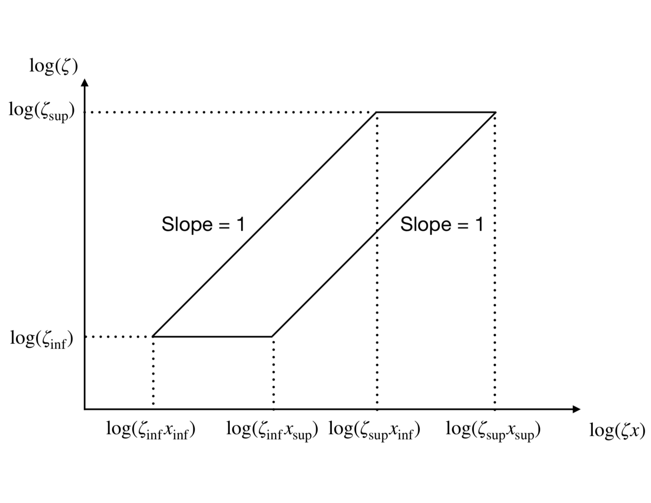
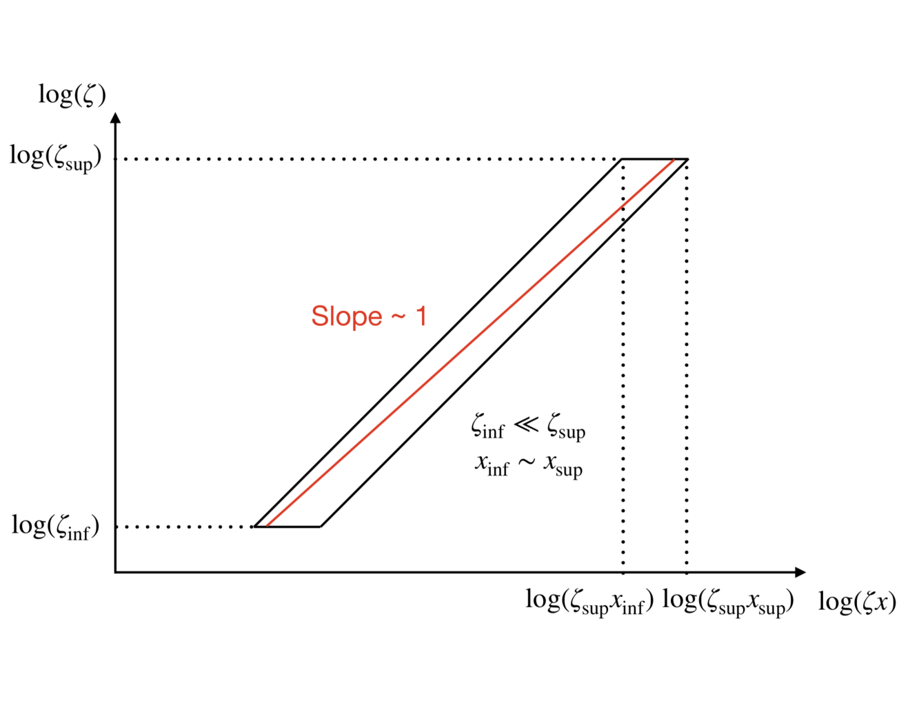
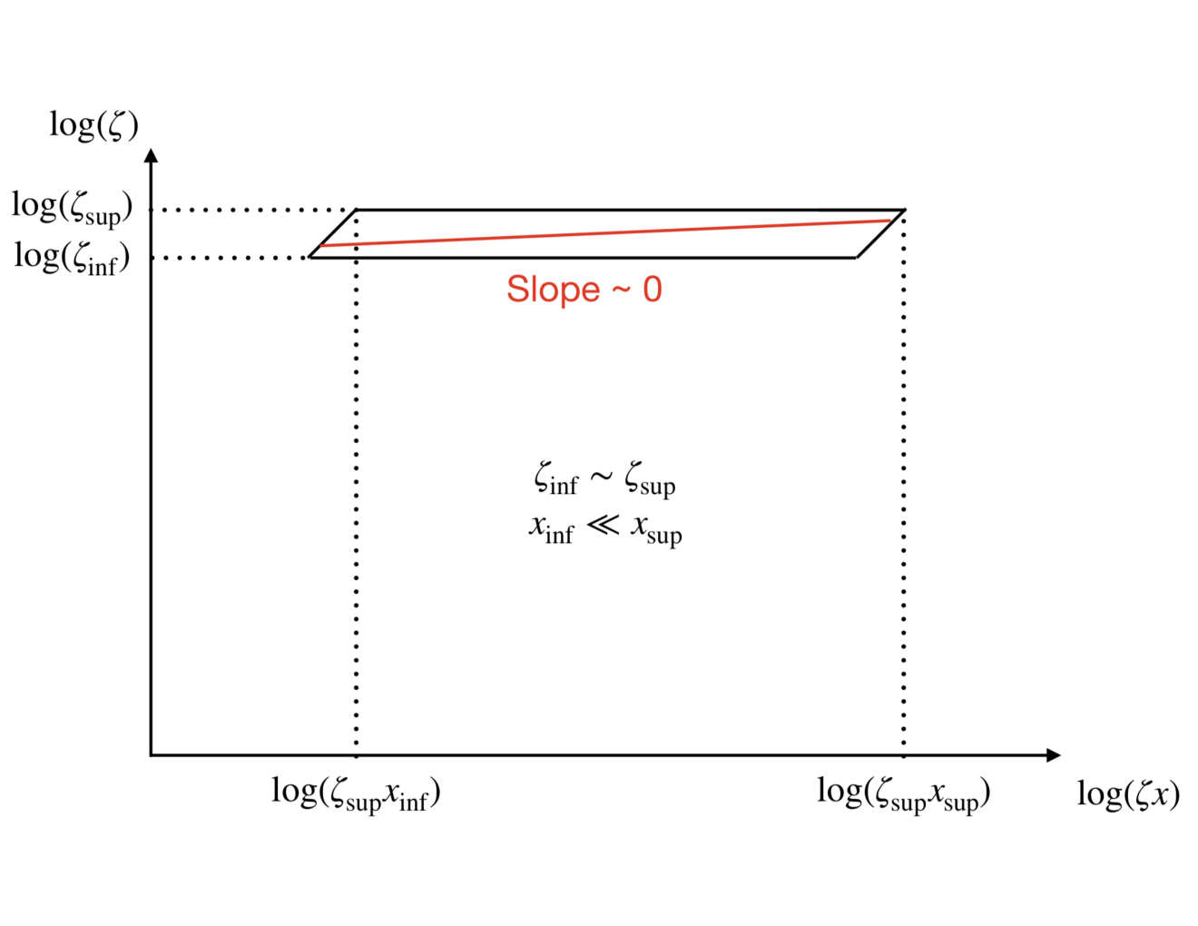
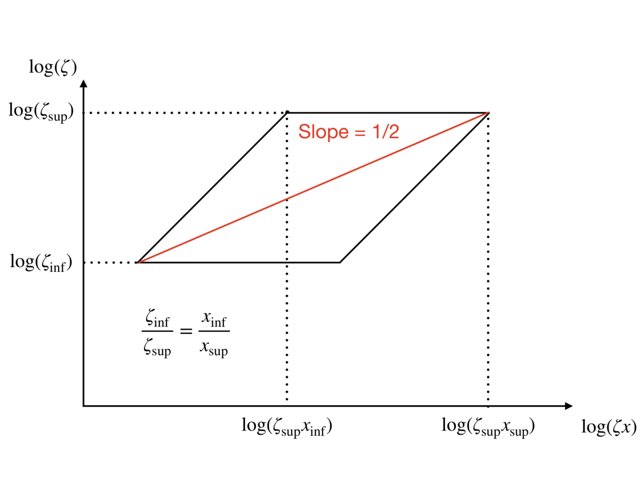
From Figure 13, we can easily see that . This inequality, in conjunction with the set of Equations (C13), leads to the immediate conclusion that for the linear transformation we have just presented will result in a best-fit relation that is closer to unity, while increasing the dispersion of the data around this best-fit.
Now let us assume that both and are random variables uniformly distributed in the intervals and (see top left panel of Figure 13). If and , the slope of the best fit of is 1 (see top right panel of Figure 13), and Equation (C10) becomes . If and , the slope of the best fit of is 0 (see bottom left panel of Figure 13), and Equation (C10) becomes . If = , the slope of the best fit of is 1/2 (see bottom right panel of Figure 13) , and Equation (C10) becomes , which means that after random distributions of and (with the same factor, , multiplying both coordinates for each data point) the best fit slope is closer to unity, decreasing the difference by half. To test this analytical prediction we created mock representations of the – relation, which are presented in the next section.
C.2 Mock representations of the – relation
To test the analytical prediction presented in the previous section, we created mock representations of the – relation, using 200 data points. Initially, we populated the – relation with values in a similar range as presented in Figure 12 to mimic the – relation when expressed in apparent flux (units of arcmin2). We then randomly re-distributed the data points using a random variable uniformly distributed in the range to mimic the values presented in the – relation when expressed in intrinsic properties (units of Mpc2). The mock representations of the – relation are presented in Figure 14. As we can see, the best-fit results agree perfectly with the analytical prediction () presented in Section C.1 (see Table 6).
| Predicted | ||||
|---|---|---|---|---|
| 1.00 | 0.01 | 1.00 | 0.01 | 1.00 |
| 0.90 | 0.01 | 0.95 | 0.01 | 0.95 |
| 0.80 | 0.01 | 0.90 | 0.01 | 0.90 |
| 0.70 | 0.01 | 0.86 | 0.02 | 0.85 |
Note. — Columns list best fit slopes and their uncertainties for the power-law fit to the –relation expressed in apparent flux (units of arcmin2), intrinsic properties (units of Mpc2), and the predicted value given by = + (1-.
C.3 Predicted vs. observed change in slope for our sample
Finally, we investigate the predicted change in slope for our sample, using the factors () that were used for the conversion from apparent flux (units of arcmin2) to intrinsic properties (units of Mpc2). Using the notation of Section C.1 and starting from the – relation expressed in apparent flux (units of arcmin2), we have:
- •
and ;
- •
and ;
- •
= slope of the best fit of the – relation in apparent flux (units of arcmin2) and = slope of the best fit of the – relation in intrinsic properties (units of Mpc2).
Using the formalism presented in Section C.1 and the variables as defined above, the predicted slope of the best fit of the – relation when changed from apparent flux (units of arcmin2) to intrinsic properties (units of Mpc2) is given by Equation (C10), where the term multiplying is the slope of the best fit of the () – relation (–) in logarithmic space, which turns out to be 0.85 (see bottom panel of Figure 15). This leads to a predicted slope of the best fit of the – relation in intrinsic properties of = 0.98, which is in agreement with the the observed value of . Now, if we perform the same calculation to compute the predicted value of the slope of the –in apparent flux starting from this relation in intrinsic properties (the slope of the best fit of – is 0.90 – see bottom panel of Figure 15), we obtain: = 1.00, which is in total disagreement with the observed value of .
The question that then arises naturally is why going from apparent flux to intrinsic properties results in a slope that is closer to unity, and yet the reverse is not the case.
Based on the analytical formalism presented in Section C.1, we know that any re-ordering of the data will result in a slope that is closer to unity. However, the analytical formalism does not indicate any mathematical property that allows us to know the direction that this transformation results in a slope that is closer to unity.
The answer to this question seems to be given by understanding what is first observed, therefore what is the starting point. The observed integrated Compton parameter () is measured from the apparent flux (arcmin2) from the Planck data. Similarly, the X-ray equivalent of the integrated Compton parameter, , which is given by the product of a gas mass and a gas temperature, has a cosmological dependence on the gas mass, which is originally measured from the observed emission measure profile, and which is therefore also dependent on the apparent flux. It is only after calculations involving the underlying cosmology and cluster redshift that is presented in intrinsic properties ( or Mpc2). Based on this reasoning, we see that the starting point is given by measurements that involve the apparent flux. Therefore, going from apparent flux (units of arcmin2) to intrinsic properties (units of Mpc2) should result in a best-fit slope that is closer to unity according to our analytical formalism presented in Section C.1. This is indeed what we observe.

