Hamiltonian Monte Carlo in Inverse Problems; Ill-Conditioning and Multi-Modality.

Consider the toy problem

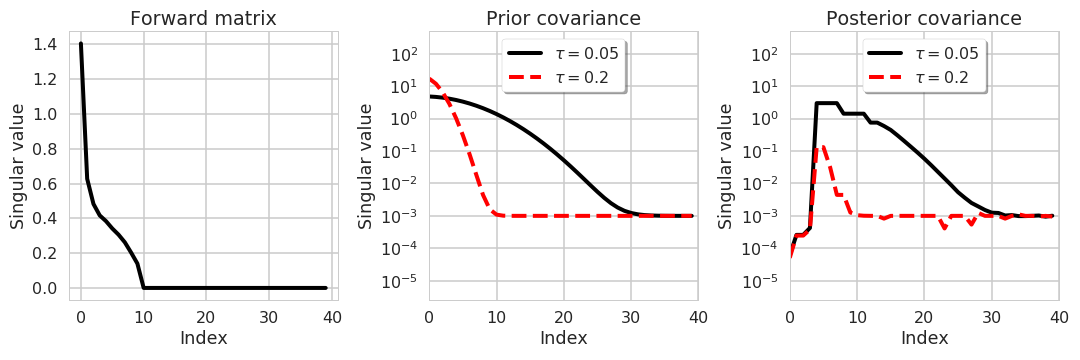
where $A\in{{\mathbb{R}}^{M\times N}}$ is the forward matrix, mapping the unknown state variable $X$ to the measurement space ${\mathbb{R}}^{M}$. The prior correlation, $C_{pr}$, is the discretization of (5). Collecting terms quadratic in $x$, the posterior covariance is

Suppose the forward matrix $A$ is low rank, and so only constrains $M<N$ directions in ${\mathbb{R}}^{N}$. For small $\sigma$, these constrained directions will have small posterior variance asymptotic to $\sigma^{2}$. The other directions will have variance governed by $C_{pr}$. The result is poorly conditioned posterior covariance. See figure 1. In that example, sampling is about 92 times less efficient than if the posterior was ideally conditioned. Section 3.4 details the relationship between sampling efficiency and conditioning.

The posterior corresponding to the linear problem from section 2.1 will always have exactly one local maximum, or mode. In practice, non-linear parameterizations of state can easily lead to multiple modes. These tend to arise in an attempt to model details that are not fully constrained by the data.

A multi-modal toy model is a Gaussian prior for $X\in{\mathbb{R}}^{N}$ and mixture of Gaussians likelihood corresponding to $M\leq N$ measurements.

This leads to posterior density

When $\sigma\ll 1$, standard HMC will find itself stuck in any of the $2^{M}$ modes. The probability of escaping one of these modes is, to leading order, less than $\exp\left\{-(1+\sigma^{2})/\sigma^{2}\right\}$. See section 3.5.

Our model problem is the inference of amplitude, temperature, and velocity of an ion species from an emission spectrum. Photons are emitted from an N-point discretization of the square $[-1,1]\times[-1,1]$, and line integrated emission is measured. Some details are given, so as to emphasize the ability of HMC to handle non-Gaussian posteriors. Other sections do not require understanding of these details.

For a set of (around 200) frequencies $\nu$, we parameterize emissivity as a transformation, $\varphi_{\nu}$, of an a-priori Gaussian random variable $X\in{\mathbb{R}}^{N}$, $X\sim{\mathcal{N}}(0,C_{pr})$. At each frequency $\nu$, an integration matrix ${\mathcal{I}}\in{{\mathbb{R}}^{M\times N}}$ projects the emissivity $\varphi_{\nu}(X)$ onto $M$ measurements. This models $M$ distinct view chords in the $[-1,1]\times[-1,1]$ square (Fig. 2).

The noise $\eta_{\nu}\in{\mathbb{R}}^{M}$ is, conditional on $X$, Gaussian, and independent for every frequency and chord. It takes the form

The factor $\sigma$ gives rise to the usual additive independent noise. $\sigma_{p}$ gives us noise proportional to the signal, representing model error. This leads to the likelihood

The mapping $\varphi_{\nu}$ is composed of two stages. First, $X$ is divided into independent amplitude, temperature, and velocity components; $X=(X_{\mathcal{A}},X_{\mathcal{T}},X_{\mathcal{V}})$. These are mapped to amplitude $\mathcal{A}$, temperature $\mathcal{T}$, and velocity $\mathcal{V}$. The mapping is either slab, meaning constant on chord-aligned rectangles, or shell, meaning constant on circles of rotation, about a shifted center (Fig. 2).

To make amplitude and temperature positive, we use the softplus function; ${\mathcal{S}}(u):=\log[1+exp\left\{u\right\}]$.

Above, $(c_{\mathcal{A}},c_{\mathcal{T}},c_{\mathcal{V}})$ are scaling factors, and $\tilde{X}:=(\tilde{X}_{\mathcal{A}},\tilde{X}_{\mathcal{T}},\tilde{X}_{\mathcal{V}})$ is a transformation of $X$ to impart radial correlation and a shifted center. That is, the amplitude, temperature, and velocity components of $\tilde{X}$ have radial values approximating a zero mean Gaussian random field with correlation

Above, $\delta>0$ is a shrinkage parameter preventing small eigenvalues from creating numerical difficulties. The coordinate $r$ is the radius about a center shifted by an a-priori 2-D Normal.

The second step of $\varphi_{\nu}$ is the dimensionless discrete emissivity spectrum.

where $\tilde{\nu}=\nu_{0}/(1-\mathcal{V})$ is the Doppler shifted center frequency, and $w=\sqrt{\mathcal{T}}/\nu_{0}$ is the Doppler broadened bandwidth.

In its shell parameterization, the spectroscopy problem can suffer from ill-conditioned posterior covariance. The Gaussian toy problem (1) is a linearization, achieved by assuming amplitude $\mathcal{A}$ is the only unknown, ignoring the softplus, and setting $\sigma_{p}=0$ and $c_{\mathcal{A}}=1$.

Multi-modality can also occur. Suppose the measured emissivity $Y_{\nu}$ has two spectral peaks at $\nu_{1}$ and $\nu_{2}$, as a result of Carbon III and an additional, unexpected, pollutant. As a result, we are trying to fit two peaks with a model capable of producing only one. This results in five different posterior modes (Fig. 3).

Changing velocity determines the Doppler shift, and therefore the mode a sample is closest to. In a neighborhood of each mode, the log-posterior is concave. In this way our spectroscopy problem is similar to the toy model (3) with the number of velocity variables, $M$, equal to $N/3$.

Samples from the Markov Chain have two major deficiencies. First, only in the limit $k\to\infty$ can we say that $X^{k}\sim\pi$. Often, a chain is initialized with a draw from the prior, and an initial burn-in period is used to allow the chain to “forget” this initial position and move toward the typical set of the posterior [15]. Second, draws are correlated. Roughly speaking, we say that identically distributed samples $\left\{X^{1},\ldots,X^{K}\right\}$ have effective sample size (ESS) $S$ if the variance of $K^{-1}\sum_{k=1}^{K}X^{k}$ is $\mbox{Var}\left\{X^{1}\right\}/S$. In other words, if, for purposes of computing the mean, they are “as effective” as $S$ i.i.d. samples. Usually $S\leq K$. The most straightforward computation of ESS assumes the $\{X^{k}\}$ are identically distributed but correlated draws from the target, with mean $\mu$ and variance $\nu^{2}$. Then, for dimensions $n=1,\ldots,N$, ESS is built from the $t-$lag autocorrelation $\rho_{t}$,

We are are usually most interested in the worst performing dimension, and therefore ${\min_{n}\left\{\mathrm{ESS_{n}}\right\}}$. Due to insufficient burn-in, or being stuck in local modes, the assumption that $X^{k}$ are draws from the target is often not satisfied. For that reason, our version of ESS will be lower if the mean differs between multiple chains. See appendix A of [16]. A more direct method of checking deviation between chains is the potential scale reduction, or ${\hat{R}}$ [16].

In our experience, obtaining MCMC samples on production models is a computationally intensive task that can take prohibitively long.

Graphical processing units (GPUs) provide a significant speedup, as they excel at parallel (SIMD) operations. This allows concurrent running of multiple Markov Chains [17]. The slowdown as more chains are added is sub-linear, until GPU memory is exhausted. We therefore only consider algorithms that take advantage of GPU parallelism. In particular, our replica-exchange implementation uses the same number of leapfrog steps for each replica (see section 5.3.4).

The majority of HMC computation time is spent in the numerical (leapfrog) integration of Hamilton’s equations. Accordingly, we track the number of leapfrog steps per effective sample (${\min_{n}\left\{\mathrm{ESS_{n}}\right\}}$ actually) as a performance metric. This allows platform independent comparisons.

A secondary performance consideration is time spent compiling and optimization the computational graph [18, 19]. This takes a fixed amount of time proportional to the graph complexity. In our model problem, where ill-conditioning and/or multi-modality was present, graph optimization was a small fraction of total runtime. In well-conditioned HMC sampling problems, avoiding many graph optimizations may be important.

The Hamiltonian Monte Carlo (HMC) method was introduced in 1987 as “Hybrid Monte Carlo” for use in lattice field theory simulations [20]. Since then, it has been recognized as an efficient alternative to random walk Metropolis-Hastings, well suited for higher dimensional problems. Implementations are available for a variety of languages [21, 17, 22]. A comprehensive introduction to HMC can be found in [1].

To sample $X\in{\mathbb{R}}^{N}$, distributed according to a smooth (with respect to Lebesgue measure) density $\pi(x)$, HMC augments state space with a fictitious momentum $\xi\in{\mathbb{R}}^{N}$. This defines the joint density

and $\|\xi\|$ is the Euclidean norm. In the physics setting, the Hamiltonian $H$ is total energy, whereas $-\log\pi(x)$, $\|\xi\|^{2}/2$ are potential and kinetic energies. It is not uncommon to model the kinetic energy $\sqrt{\xi\cdot A^{-1}\xi}/2$, where $A\in{{\mathbb{R}}^{N\times N}}$ is the mass matrix. However, as shown in section 4 of [1], this is equivalent to the linear preconditioning $X\mapsto LX$ (where $A^{-1}=LL^{T}$) in conjunction with the Euclidean norm. Kinetic energy can be non-Gaussian e.g. depend on position [23]. See also [15].

Sampling proceeds by (a numerical approximation to) the following iteration from point $(x^{j},\xi^{j})$.

1. 1.

   Draw $\tilde{\xi}\sim{\mathcal{N}}(0,I_{N})$.

2. 2.

   Let $(x(t),\xi(t))$ be the time $t$ solution to the Hamilton’s equations of motion:  $\dot{x}=\xi$, $\dot{\xi}=\nabla\log\pi(x)$, with initial condition $(x^{j},\tilde{\xi})$.

3. 3.

   Set $(x^{j+1},\xi^{j+1})=(x(t),\xi(t))$, for integration time $t$.

Each integration path lives on a single level set of the Hamiltonian. The resampling step $\tilde{\xi}\sim{\mathcal{N}}(0,I_{N})$ is necessary to jump between level sets, and is thus necessary for ergodicity [24].

In practice, Hamilton’s equations must be solved numerically over $\ell$ steps with step-size $h$. Denote this solution by $\Psi^{\ell}$. The integration error means we can no longer just accept the move in step 3, which is replaced by a Metropolis correction:

and

for acceptance probability

Since Hamilton’s equations preserve the Hamiltonian, if numerical integration was perfect, $H(x^{j},\xi^{j})=H(\Psi^{\ell})$ and every step would be accepted. In practice, finite step size leads to some rejections and wasted effort. We also note that for the Metropolis correction to be symmetric, the final momentum should be negated before evaluating $H$. This makes no difference since our Hamiltonian is symmetric in momentum.

The numerical integration is usually done with $\ell$ steps of the Störmer-Verlet or leapfrog integrator. This symplectic integrator ensures that the Hamiltonian does not diverge, provided $h$ is sufficiently small. See [25], theorem 8.1.

Here we review existing scaling laws for HMC step size. These results always inform our choice of HMC step size and integration time. They are directly used in section 4.

The step size $h$, along with the number of leapfrog steps $\ell$, are two important parameters to choose. Usually, $h$ is chosen to achieve some desired acceptance rate, and $\ell$ is set to the desired integration time divided by $h$. If $h$ is too large, the average acceptance probability, $\mathrm{P}[{\mathrm{Accept}}]$, will tend to zero. On the other hand, if $h$ is too small, then too many steps $\ell$ will be required, and computational effort will be wasted. In [26, 27], $X\in{\mathbb{R}}^{N}={{\mathbb{R}}^{K}}\times\cdots{{\mathbb{R}}^{K}}$ with density $\pi(x_{1},\ldots,x_{N/K})=f(x_{1})\cdots f(x_{N/K})$ is studied in the limit $N\to\infty$. This so-called i.i.d. limit yields the result that $h$ should be tuned until $0.6\leq\mathrm{P}[{\mathrm{Accept}}]\leq 0.9$.

In the Gaussian case, we can extract more precise conclusions, resulting in useful analysis and algorithms that can be used, even in non-Gaussian problems. Consider a target $X\sim{\mathcal{N}}(0,C)$, where $C$ has eigenvalues $\lambda_{1}^{2}\geq\lambda_{2}^{2}\geq\cdots\geq\lambda_{N}^{2}>0$. If we want the integration trajectories to travel a distance comparable to the largest scale $\lambda_{1}$, we must have $h\ell=O(\lambda_{1})$. On the other hand, to avoid instability, we must have $h\leq 2\lambda_{N}$. This leads to a naive scaling $\ell=O(\lambda_{1}/\lambda_{N})$. The ratio $\lambda_{1}/\lambda_{N}$ is the common, spectral, condition number of any matrix $L$ such that $C=LL^{T}$.

The problem with the spectral condition number is that it takes into account only the largest and smallest scales. The largest scale does set the required integration length, but all dimensions contribute to integration error. A condition number taking these considerations into account was introduced in [28].

Above, $\|\cdot\|_{2}$ is the spectral norm, and $\|\cdot\|_{S^{4}}$ is the fourth Schatten norm [29]. For matrix $A$ with singular values $\lambda_{1}\geq\cdots\lambda_{N}\geq 0$, the $k^{th}$ Schatten norm is

In [28], it is shown that under some regularity conditions, a Gaussian density requires $O({\kappa})$ leapfrog steps for efficient sampling. ${\kappa}$ may be approximated using the largest scale $\lambda_{1}$, step size $h$, and average acceptance probability $\mathrm{P}[{\mathrm{Accept}}]$.

Above, $\Phi$ is the normal cumulative distribution function. Thus, ${\kappa}$ is the number of steps needed to traverse the largest scale, $\lambda_{1}/h$, times a correction factor depending on acceptance probability. In non-Gaussian problems, we recommend using large (small) $\lambda_{1}/h$ as evidence of possible of inefficient (efficent) sampling.

Let $A\subset{\mathbb{R}}^{N}$, and $c(A)$ the average probability of the chain escaping $A$ in one step. The conductance of the chain, $\mathcal{C}:=\min_{\pi(A)<1/2}\{c(A)\}$, quantifies its ability to escape local modes. In [30], it is shown that the conductance of HMC is no better than that of random walk Metropolis-Hastings. An upper bound is also given for conductance of HMC chains:

From (11) it is clear that increasing integration time can increase conductance at most linearly. Since computational effort also increases linearly with $t$, this does not help overall.

Equation (11) also shows that conductance can be constricted by a single low-probability (density) surface. For Gaussian noise models (e.g. section 2.3), this can lead to conductance decreasing exponentially in $1/\sigma^{2}$. Indeed, for the bi-modal normal $0.5\,{\mathcal{N}}(-1,\sigma^{2})+0.5\,{\mathcal{N}}(1,\sigma^{2})$, the leading order term of conductance is proportional to $\exp\left\{-1/(2\sigma^{2})\right\}$. See [30] theorem 3.

Tempering methods need to use a highest temperature ${T_{max}}$ such that the corresponding “hottest density” has non-vanishing conductance. See section 5.3.2.

Here we write some relations involving pushforwards by diffeomorphisms. They will be needed in later sections.

Let us start with $X\sim p(\cdot{\,|\,}y)$, and a diffeomorphism $F$, which transforms $X\mapsto Z=F^{-1}(X)$. Equivalently, the density $p(\cdot{\,|\,}y)$ is transformed by the pushforward operator, ${F^{-1}_{\#}}$, into $g$:

Above, $DF$ is the matrix of partial derivatives, $(DF)_{ij}=\partial F_{j}/\partial z_{i}$. Using HMC, we sample from the transformed density $g$, producing $Z^{1},\ldots,Z^{K}$. Transforming back, $X^{k}:=F(Z^{k})$, and we have samples from $p(\cdot{\,|\,}y)$ as desired.

In the Gaussian case, $p(\cdot{\,|\,}y)\sim{\mathcal{N}}(\mu,C)$, with $C=LL^{T}$, the linear preconditioner induced by a matrix $F$ transforms $L\mapsto F^{-1}L$, and likewise the covariance and ${\kappa}$ as

If the support of ${p(x{\,|\,}y)}$ is bounded, sampling directly from it will suffer from boundary issues. It is therefore standard practice to transform $X\to Z:=F^{-1}(X)$ (as in section 4.1) such that ${\mbox{supp}}(Z)={\mathbb{R}}^{N}$. We know of no existing work analyzing the effects of this reparameterization on conditioning, so we include it here.

In our case, the prior $p(x)$ is a transformation of a standard Gaussian by a diffeomorphism $G$. That is, $p(x)=({G_{\#}}\phi)(x)$. This means $Z=G^{-1}(X)$ is a useful transformation. If the prior results in difficult posterior covariance (see e.g. section 2.1), using $G$ as a preconditioner will often improve conditioning. To that end, note that

Thus, preconditioning with $G$ is equivalent to a reparameterization that uses a standard Gaussian prior, and inserts $G$ inside the likelihood (probably achieved by using $G(x)$ in the forward model). In our work, we sometimes explicitly preconditioned with $G$, and at other times reparameterized a unit normal. Not only are these mathematically equivalent, but, due to caching in TensorFlow probability, they are computationally equivalent ($G\circ G^{-1}$ is replaced by the identity) [31]. Doing one of these is necessary, as it removes much of the nonlinearity and allows the methods of section 4.3 to work efficiently.

Organizing code around reparameterizations has some advantages: First, the benefits of preconditioning by the prior are realized without the programmatic complexity of specifying a preconditioner. Second, the function $G$ does not need to be a diffeomorphism; see [5] for an example. On the other hand, there are benefits to letting the prior encode the state directly. First, in this setup, the MCMC variables being sampled are the state variables you care about. Second, one can use a prior not easily described as a transformation of a Gaussian.

The sampling benefits/degradation of prior-reparameterization will vary. Consider the Gaussian example (1). If $C_{pr}=L_{pr}L_{pr}^{T}$, then the reparameterized posterior covariance becomes

We see in figure 4 that reparameterization can help when prior covariance is the major contributor to ${\kappa}$, but can hurt if low noise is the major source of small eigenvalues.

Here we examine linear preconditioning of Gaussian distributions. This simplification allows for precise results and inspires techniques. These techniques are applied to non-Gaussian problems in section 4.4.

The setup here is like other diffeomorphisms (section 4.1), except we assume $X\sim{\mathcal{N}}(0,C)$ is Gaussian, and the preconditioning transformation $F\in{{\mathbb{R}}^{N\times N}}$ is linear. If $FF^{T}$ is a scalar multiple of $C$, then (13) shows the transformed covariance is a multiple of the identity, which minimizes ${\kappa}$. Subsequent sections will use approximations of this factor built from samples obtained during burn-in.

Here we compare preconditioning schemes as applied to the shell model from section 2.3. This problem is non-Gaussian. In particular, the noise level depends on the signal, the temperature and amplitude are constrained to be positive via a Softplus, the coordinate system is shifted, and emissivity is a nonlinear function. This is still “weakly” non-Gaussian, since observed skew and kurtosis levels of transformed samples $Z$ were close to that of a Normal.

The schemes compared are referred to as “full”, “diag”, and “none”. “Full” uses algorithm 1. “Diag” uses algorithm 1 but skips the NUTS sampling and uses diagonal rather than sample covariance preconditioning. “None” does not precondition. Code was run on Tesla P100 GPUs.

20 plasmas to reconstruct were drawn from the prior. The reconstruction model used a variety of noise levels from $\sigma=1.25$ to 15. Each reconstruction was run until ${\min_{n}\left\{\mathrm{ESS_{n}}\right\}}=S_{f}$, for $S_{f}\in\left\{400,1600,6400\right\}$. A total of 282 reconstruction configurations were attempted for each of the three schemes. Eleven configurations were thrown out, since at least one model failed to reduce ${\hat{R}}$ fast enough. This is usually the result of being stuck in a local mode due to poor initialization. If this happens in production, our algorithm re-starts with REMC. The traces in figure 6 help visualize different stages of algorithm 1. Figure 7 shows ${\kappa}$ correlates well with sampling efficiency, and can be predicted from proposition 4.4, even in this non-Gaussian problem. Figure 8 shows that the full preconditioner significantly speeds up sampling, at the cost of a more expensive burn-in. Diagonal preconditioning helps only a little.

This section reviews REMC (also known as parallel tempering). Related techniques, such as annealed importance sampling, also deserve consideration [37].

Given posterior ${p(x{\,|\,}y)}\propto{p(x)}{p(y{\,|\,}x)}$, and sequence of temperatures $1=T_{1}<T_{2}<\cdots<T_{R}\leq\infty$, we form the replica densities $\pi_{r}$ in one of two ways.

To gain intuition, consider the unimodal example where the prior $p(x)\sim{\mathcal{N}}(0,I)$ and the likelihood $p(y{\,|\,}x)\sim{\mathcal{N}}(\mu,\Gamma)$. The posterior covariance after tempering with $T$ will be

Posterior tempering increases posterior variance without changing the shape or condition number. Likelihood tempering distorts the posterior covariance to make it look like the prior. See figure 9.

Together, these form the joint density $\pi(x_{1},\ldots,x_{R}):=\pi_{1}(x_{1})\cdots\pi_{R}(x_{R})$. Samples from $(X_{1}^{k},\ldots,X_{R}^{k})\sim\pi$ are generated, but only the target samples $X_{1}^{k}\sim\pi_{1}=p(\cdot{\,|\,}y)$ are kept. REMC repeats two alternating steps. In the exploration step, each replica progresses independently, $X^{k-1}_{r}\to X^{k}_{r}$. HMC, or another sampling method, can be used here. In the communication step, a number of swaps are proposed between adjacent replicas. For example, the $(1,2)$ swap proposes that replicas 1 and 2 exchange position; $X^{k+1}_{1}=X^{k}_{2}$ and $X^{k+1}_{2}=X^{k}_{1}$. The set of swaps proposed at each turn are either the set of even swaps $\left\{(1,2),(3,4),\ldots\right\}$, or odd swaps $\left\{(2,3),(4,5),\ldots\right\}$. In both cases, each swap is independently accepted or rejected according to the standard Metropolis-Hastings criteria. For example,

The computational cost of swapping is negligible compared with leapfrog integration. We therefore propose swaps between every exploration step. In most of the literature, swaps are proposed using a stochastic even-odd (SEO) scheme, whereby a coin flip chooses between even and odd swaps. More recently, deterministically alternating between even and odd swaps was proposed [38]. This deterministic even odd scheme (DEO) scheme has superior scaling characteristics [39]. We use DEO in all experiments.

Effective REMC requires the mean swap probabilities,

be large enough to allow information from the hottest replica (the replica using the highest temperature) to make its way to the target. This section shows that, unlike conductance, swap probability is strongly related to dimension.

References

- [1] Radford Neal. MCMC using Hamiltonian dynamics. In Brooks, S. and Gelman, A. and Jones, G. and Meng, X.L., editor, Handbook of Markov Chain Monte Carlo, volume 54, pages 113–162. CRC Press, May 2011.
- [2] Andreas Fichtner, Andrea Zunino, and Lars Gebraad. Hamiltonian Monte Carlo solution of tomographic inverse problems. Geophys. J. Int., 216(2):1344–1363, February 2019.
- [3] T Bui-Thanh and M Girolami. Solving large-scale PDE-constrained Bayesian inverse problems with Riemann manifold Hamiltonian Monte Carlo. Inverse Probl., 30(11):114014, October 2014.
- [4] Nagel Joseph B. and Sudret Bruno. Hamiltonian Monte Carlo and Borrowing Strength in Hierarchical Inverse Problems. ASCE-ASME Journal of Risk and Uncertainty in Engineering Systems, Part A: Civil Engineering, 2(3):B4015008, September 2016.
- [5] Michael Dikovsky, Edward A Baltz, Robert Von Behren, Scott Geraedts, Anton Kast, Ian Langmore, Thomas Madams, Peter Norgaard, John C Platt, Jesus Romero, Thomas Roche, Roger Smith, Erik Trask, Sean Dettrick, Hiroshi Gota, James B Titus, and Richard M Magee. Multi-instrument Bayesian reconstruction of plasma shape evolution in the C-2W experiment. Phys. Plasmas, 28(6):062503, June 2021.
- [6] Dennis Conway, Janelle Simpson, Yohannes Didana, Joseph Rugari, and Graham Heinson. Probabilistic Magnetotelluric Inversion with Adaptive Regularisation Using the No-U-Turns Sampler. Pure Appl. Geophys., 175(8):2881–2894, August 2018.
- [7] Alexandros Beskos, Frank J Pinski, Jesus-Maria Sanz-Serna, and Andrew M Stuart. Hybrid Monte Carlo on Hilbert spaces. Stochastic Process. Appl., 121(10):2201–2230, October 2011.
- [8] Khai Xiang Au, Matthew M Graham, and Alexandre H Thiery. Manifold lifting: scaling MCMC to the vanishing noise regime. Arxiv preprint, https://arxiv.org/abs/2003.03950, March 2020.
- [9] Michael Betancourt, Simon Byrne, Sam Livingstone, and Mark Girolami. The geometric foundations of Hamiltonian Monte Carlo. Bernoulli, 23(4A):2257–2298, November 2017.
- [10] D Calvetti and E Somersalo. Inverse problems: From regularization to Bayesian inference. WIREs Comput Stat, 10(3):e1427, May 2018.
- [11] Andrew Gelman, Aki Vehtari, Daniel Simpson, Charles C Margossian, Bob Carpenter, Yuling Yao, Lauren Kennedy, Jonah Gabry, Paul-Christian Bürkner, and Martin Modrák. Bayesian Workflow. Arxiv preprint, https://arxiv.org/abs/2011.01808, November 2020.
- [12] Ian Goodfellow, Yoshua Bengio, and Aaron Courville. Deep Learning. MIT Press, November 2016.
- [13] Sebastian Farquhar, Lewis Smith, and Yarin Gal. Liberty or Depth: Deep Bayesian Neural Nets Do Not Need Complex Weight Posterior Approximations. In H. Larochelle and M. Ranzato and R. Hadsell and M.F. Balcan and H. Lin, editor, Advances in Neural Information Processing Systems, pages 4346–4357, February 2020.
- [14] Christian Robert and George Casella. A Short History of Markov Chain Monte Carlo: Subjective Recollections from Incomplete Data. Stat. Sci., 26(1):102–115, 2011.
- [15] Michael Betancourt. A Conceptual Introduction to Hamiltonian Monte Carlo. January 2017.
- [16] Aki Vehtari, Andrew Gelman, Daniel Simpson, Bob Carpenter, and Paul-Christian Bürkner. Rank-normalization, folding, and localization: An improved Rˆ for assessing convergence of MCMC (with discussion). Bayesian Anal., 16(2), June 2021.
- [17] Junpeng Lao, Christopher Suter, Ian Langmore, Cyril Chimisov, Ashish Saxena, Pavel Sountsov, Dave Moore, Rif A Saurous, Matthew D Hoffman, and Joshua V Dillon. tfp.mcmc: Modern Markov Chain Monte Carlo Tools Built for Modern Hardware. Arxiv preprint, https://arxiv.org/abs/2002.01184, February 2020.
- [18] Martín Abadi, Ashish Agarwal, Paul Barham, Eugene Brevdo, Zhifeng Chen, Craig Citro, Greg S. Corrado, Andy Davis, Jeffrey Dean, Matthieu Devin, Sanjay Ghemawat, Ian Goodfellow, Andrew Harp, Geoffrey Irving, Michael Isard, Yangqing Jia, Rafal Jozefowicz, Lukasz Kaiser, Manjunath Kudlur, Josh Levenberg, Dandelion Mané, Rajat Monga, Sherry Moore, Derek Murray, Chris Olah, Mike Schuster, Jonathon Shlens, Benoit Steiner, Ilya Sutskever, Kunal Talwar, Paul Tucker, Vincent Vanhoucke, Vijay Vasudevan, Fernanda Viégas, Oriol Vinyals, Pete Warden, Martin Wattenberg, Martin Wicke, Yuan Yu, and Xiaoqiang Zheng. TensorFlow: Large-Scale Machine Learning on Heterogeneous Systems. Technical report, 2015.
- [19] Roy Frostig, Matthew James Johnson, and Chris Leary. Compiling machine learning programs via high-level tracing. https://mlsys.org/Conferences/2019/doc/2018/146.pdf. Accessed: 2022-1-2.
- [20] Simon Duane, A D Kennedy, Brian J Pendleton, and Duncan Roweth. Hybrid Monte Carlo. Phys. Lett. B, 195(2):216–222, 1987.
- [21] Bob Carpenter, Andrew Gelman, Matthew D Hoffman, Daniel Lee, Ben Goodrich, Michael Betancourt, Marcus Brubaker, Jiqiang Guo, Peter Li, and Allen Riddell. Stan: A Probabilistic Programming Language. J. Stat. Softw., 76(1), 2017.
- [22] John Salvatier, Thomas V Wiecki, and Christopher Fonnesbeck. Probabilistic programming in Python using PyMC3. PeerJ Comput. Sci., 2:e55, April 2016.
- [23] Mark Girolami and Ben Calderhead. Riemann manifold Langevin and Hamiltonian Monte Carlo methods. Journal of the Royal Statistical Society: Series B (Statistical Methodology), 2011.
- [24] Samuel Livingstone, Michael Betancourt, Simon Byrne, and Mark Girolami. On the Geometric Ergodicity of Hamiltonian Monte Carlo. Arxiv preprint, https://arxiv.org/abs/1601.08057, January 2016.
- [25] Ernst Hairer, Christian Lubich, and Gerhard Wanner. Geometric Numerical Integration: Structure-Preserving Algorithms for Ordinary Differential Equations. Springer, February 2006.
- [26] Alexandros Beskos, Natesh Pillai, Gareth Roberts, Jesus-Maria Sanz-Serna, and Andrew Stuart. Optimal tuning of the hybrid Monte Carlo algorithm. Bernoulli, 19(5A):1501–1534, November 2013.
- [27] Michael Betancourt, Simon Byrne, and Mark Girolami. Optimizing The Integrator Step Size for Hamiltonian Monte Carlo. November 2014.
- [28] Ian Langmore, Michael Dikovsky, Scott Geraedts, Peter Norgaard, and Rob Von Behren. A Condition Number for Hamiltonian Monte Carlo. Arxiv preprint, https://arxiv.org/abs/1905.09813, February 2020.
- [29] Roger A Horn, Roger A Horn, and Charles R Johnson. Matrix Analysis. Cambridge University Press, February 1990.
- [30] Oren Mangoubi, Natesh S Pillai, and Aaron Smith. Does Hamiltonian Monte Carlo mix faster than a random walk on multimodal densities? August 2018.
- [31] Joshua V Dillon, Ian Langmore, Dustin Tran, Eugene Brevdo, Srinivas Vasudevan, Dave Moore, Brian Patton, Alex Alemi, Matt Hoffman, and Rif A Saurous. TensorFlow Distributions. Arxiv preprint, https://arxiv.org/abs/1711.10604, November 2017.
- [32] Zhidong Bai. Methodologies in spectral analysis of large dimensional random matrices, a review. Statistica Sinica, 9(3):611–662, 1999.
- [33] Arup Bose, Sreela Gangopadhyay, and Arnab Sen. Limiting spectral distribution of XX’ matrices. Ann. Inst. Henri Poincare Probab. Stat., 46(3):677–707, August 2010.
- [34] Matthew D Hoffman. The No-U-Turn Sampler: Adaptively Setting Path Lengths in Hamiltonian Monte Carlo. Journal of Machine Learning Research, 15, 2014.
- [35] Christophe Andrieu and Johannes Thoms. A tutorial on adaptive MCMC. Stat. Comput., 18(4):343–373, December 2008.
- [36] R H Swendsen and J S Wang. Replica Monte Carlo simulation of spin glasses. Phys. Rev. Lett., 57(21):2607–2609, November 1986.
- [37] Radford M Neal. Annealed importance sampling. Stat. Comput., 11(2):125–139, April 2001.
- [38] Tsuneyasu Okabe, Masaaki Kawata, Yuko Okamoto, and Masuhiro Mikami. Replica-exchange Monte Carlo method for the isobaric–isothermal ensemble. Chem. Phys. Lett., 335(5):435–439, March 2001.
- [39] Saifuddin Syed, Alexandre Bouchard-Côté, George Deligiannidis, and Arnaud Doucet. Non‐reversible parallel tempering: A scalable highly parallel MCMC scheme. J. R. Stat. Soc. Series B Stat. Methodol., 84(2):321–350, April 2022.
- [40] Sergey Bobkov and Mokshay Madiman. Concentration of the information in data with log-concave distributions. Ann. Probab., 39(4):1528–1543, July 2011.
- [41] David A Kofke. On the acceptance probability of replica-exchange Monte Carlo trials. J. Chem. Phys., 117(15):6911–6914, October 2002.
- [42] A van der Sluis. Condition numbers and equilibration of matrices. Numer. Math., 14(1):14–23, December 1969.
- [43] B Laurent and P Massart. Adaptive estimation of a quadratic functional by model selection. Ann. Stat., 28(5):1302–1338, October 2000.