跳到论文正文
W Papers独立论文阅读器 arXiv:2103.07504 论文正文 计算阅读时间 · 0%
引用这篇论文根据当前论文元数据生成,正式投稿前建议核对。


License: arXiv.org perpetual non-exclusive license
arXiv:2103.07504v4 [quant-ph] 05 Jan 2026

Improved device-independent randomness expansion rates using two sided randomness

Rutvij Bhavsar Affiliation: Department of Mathematics, University of York, Heslington, York, YO10 5DD, United Kingdom    Sammy Ragy Affiliation: Department of Mathematics, University of York, Heslington, York, YO10 5DD, United Kingdom    Roger Colbeck Email: roger.colbeck@york.ac.uk Affiliation: Department of Mathematics, University of York, Heslington, York, YO10 5DD, United Kingdom
5th5^{\text{th}} January 2026
Abstract

A device-independent randomness expansion protocol aims to take an initial random string and generate a longer one, where the security of the protocol does not rely on knowing the inner workings of the devices used to run it. In order to do so, the protocol tests that the devices violate a Bell inequality and one then needs to bound the amount of extractable randomness in terms of the observed violation. The entropy accumulation theorem lower bounds the extractable randomness of a protocol with many rounds in terms of the single-round von Neumann entropy of any strategy achieving the observed score. Tight bounds on the von Neumann entropy are known for the one-sided randomness (i.e., where the randomness from only one party is used) when using the Clauser-Horne-Shimony-Holt (CHSH) game. Here we investigate the possible improvement that could be gained using the two-sided randomness. We generate upper bounds on this randomness by attempting to find the optimal eavesdropping strategy, providing analytic formulae in two cases. We additionally compute lower bounds that outperform previous ones and can be made arbitrarily tight (at the expense of more computation time). These bounds get close to our upper bounds, and hence we conjecture that our upper bounds are tight. We also consider a modified protocol in which the input randomness is recycled. This modified protocol shows the possibility of rate gains of several orders of magnitude based on recent experimental parameters, making device-independent randomness expansion significantly more practical. It also enables the locality loophole to be closed while expanding randomness in a way that typical spot-checking protocols do not.

I Introduction

Random numbers have a wide variety of uses. In some applications, only the distribution of the random numbers matters, while in others it is important that the generated numbers are also private, for instance when used for cryptography. According to our current understanding of physics, generating fundamentally random numbers requires quantum processes. While it is easy to come up with a quantum process that can in theory generate random numbers, given a candidate quantum random number generator, verifying that it is indeed generating random numbers and at what rate is a difficult task that usually requires detailed understanding of the physical device. Any mismatch between the model of the device used in the security proof and the real device could in principle be exploited by an adversary.

Device-independent protocols aim to circumvent the mismatch problem by designing the protocol to abort unless the devices used are performing sufficiently well, and without needing to know the internal mechanism by which they operate. In the context of device-independent randomness expansion (DIRE) the main idea is that the ability to violate a Bell inequality implies that the devices doing so must be generating randomness Colbeck 2007; Colbeck and Kent 2011. Thus, in a sense, the protocol self-tests Mayers and Yao 1998 the devices during its operation, leading to enhanced security. Although challenging to accomplish, recently the first experimental demonstrations of DIRE were performed Li et al. 2021; Shalm et al. 2021; Liu et al. 2021, following earlier experiments considering randomness generation Pironio et al. 2010; Bierhorst et al. 2018; Liu et al. 2018. On the theoretical side, an increasingly sophisticated series of proofs Vazirani and Vidick 2012; Miller and Shi 2014; Miller and Shi 2017 led to the current state of the art Zhang et al. 2020; Arnon-Friedman et al. 2019. In this work we consider the proofs based on the entropy accumulation theorem Dupuis et al. 2020; Dupuis and Fawzi 2019, which establishes a lower bound on the amount of randomness after many Bell tests in terms of the von Neumann entropy of a single round achieving the observed score (see Appendix E for a precise statement). Bounds on the von Neumann entropy will hence be a focus of this work.

In a DIRE protocol, randomly chosen inputs are made to two separated devices in such a way that each device cannot learn the input chosen by the other. We use XX and YY to label the inputs and AA and BB to label the outputs, and consider an adversary with side information EE. This side information could be quantum, i.e., the general strategy has an adversary hold the EE part of a state ρA′​B′​E\rho_{A^{\prime}B^{\prime}E} where the A′A^{\prime} and B′B^{\prime} systems are held by the devices. Each input XX to the first device corresponds to a measurement on A′A^{\prime} giving outcome AA and, analogously, for each input YY to the other device there is a corresponding measurement on B′B^{\prime} with outcome BB. There are two quantities of interest, both of which depend on the post-measurement state: the first is the score in some non-local game, which is a function of the conditional distribution pA​B|X​Yp_{AB|XY}; the second is the von Neumann entropy of either one or both of the outputs. More precisely, we want to express the minimum von Neumann entropy as a function of the score. In this work we study six such von Neumann entropies: H⁡(A​B|X=0,Y=0,E)H(AB|X=0,Y=0,E), H⁡(A​B|X​Y​E)H(AB|XYE), H⁡(A​B|E)H(AB|E), H⁡(A|X=0,Y=0,E)H(A|X=0,Y=0,E), H⁡(A|X​Y​E)H(A|XYE) and H⁡(A|E)H(A|E)11 1 In the one sided cases, conditioning on YY is irrelevant, but we keep this for notational symmetry..

The difficulty in bounding these stems from the fact that a priori there is no upper bound on the dimension of the systems A′A^{\prime}, B′B^{\prime} and EE that need to be considered. For instance, for some Bell inequalities it is known that the maximum quantum violation cannot be achieved if A′A^{\prime} and B′B^{\prime} are finite dimensional Slofstra 2019, and there is evidence that this is true even in the case where XX and YY are binary and where AA and BB have three possible values Pál and Vértesi 2010. However, in the case where AA, BB, XX and YY are all binary, Jordan’s lemma Jordan 1875 implies that there is no loss in generality in considering a convex combination of strategies in which A′A^{\prime} and B′B^{\prime} are two-dimensional. This observation was used to give a tight analytic lower bound on H⁡(A|X=0,Y=0,E)H(A|X=0,Y=0,E) in terms of the CHSH score Pironio et al. 2009 and is also crucial for the present work. This analytic bound was also extended to a family of CHSH-like inequalities in Woodhead et al. 2021. As well as Jordan’s lemma, such bounds rely on a series of additional simplifications. In cases where such simplifications do not hold, alternative ways to lower bound the single-round von Neumann entropy are needed. One way is to bound it using the single-round min entropy, which can be optimized at a particular level of the semi-definite hierarchy Navascués et al. 2008. Although this method can generate numerically certified lower bounds for arbitrary protocols Brown et al. 2020, there is a significant loss in tightness when moving to the single-round min entropy. More recent methods give tighter computational bounds on the von Neumann entropy Sekatski et al. 2020; Brown et al. 2021a; Brown et al. 2021b. Forming more direct and tighter bounds is a key open problem in the field of device-independence and useful for increasing the practicality of device-independent tasks.

We discuss when each of the six entropic quantities is of most interest in Section II. In summary, the one-sided entropies are most-relevant in the context of device independent quantum key distribution (DIQKD), while using both outputs is useful for DIRE. The quantities that are conditioned on X=0X=0 and Y=0Y=0 are useful for spot-checking protocols in which particular fixed measurements (taken here to be the X=0X=0 and Y=0Y=0 measurements) are used to generate randomness/key, and where the other measurements are used only rarely to check that the devices are behaving honestly. The quantities conditioned on XX and YY are useful for analysing protocols in which the generation rounds involve multiple settings, where the input randomness is recycled, and can also be used to close the locality loophole in randomness generation. The remaining quantities, H⁡(A​B|E)H(AB|E) and H⁡(A|E)H(A|E), tell us something about the fundamental randomness based on the Bell violation, and the second of these can be useful for DIQKD protocols in which the measurement settings in the generation rounds are chosen randomly and to which an adversary, Eve, does not have access.

In Section III we discuss the computation of the von Neumann entropy bounds before giving numerically generated upper bound curves for each of the six quantities when using the CHSH game as the Bell test in Section IV. For H⁡(A|X​Y​E)H(A|XYE) and H⁡(A​B|X​Y​E)H(AB|XYE) we additionally give conjectured analytic forms for the curves. We also compute lower bounds in the cases of H⁡(A|X​Y​E)H(A|XYE) and H⁡(A​B|X=0,Y=0,E)H(AB|X=0,Y=0,E) that are tighter than those previously known and in principle converge to these quantities by increasing the accuracy of the computation. We use our bounds with the EAT to show how the potential improvement carries over to finite statistics. To do so, in Section V we consider not only the usual spot-checking type protocol, but also modified protocols. The first modification is to replace the spot-check with a biased random number generator, and the second is to remove the biasing while recycling the input randomness in order to still enable expansion. Taking the experimental conditions from Liu et al. 2021, using the two sided randomness and randomness recycling gives a rate increase of several orders of magnitude with our new bounds.

II The significance of various entropic quantities

In this section we discuss the significance of the six entropic quantities given above in the context of DIRE, noting that the one-sided quantities are also useful for DIQKD. To do so we first describe the general structure of the raw randomness generation part of a spot-checking and non-spot-checking DIRE protocol. A more complete description of the protocols is in Section V.

In a protocol without spot-checking, there are two untrusted devices, and in every round their inputs XiX_{i} and YiY_{i} are generated according to some distribution pX​Yp_{XY}. Often two independent random number generators are used for this, so that pX​Y=pX​pYp_{XY}=p_{X}p_{Y}. The generated numbers are used as inputs to the devices, which return two outputs AiA_{i} and BiB_{i} respectively. This is repeated for nn rounds generating the raw randomness 𝐀{\bf A}, 𝐁{\bf B}, where the bold font denotes the concatenation of all the outputs.

In a spot-checking protocol there is an additional step in which each round is declared to be either a test round (Ti=1T_{i}=1) or a generation round (Ti=0T_{i}=0), where test rounds occur with probability γ\gamma, which is typically small. On test rounds XiX_{i} and YiY_{i} are generated according to some distributions pX​Yp_{XY}. On generation rounds, XiX_{i} and YiY_{i} are set according to some other distribution – in this work we use the deterministic distribution Xi=Yi=0X_{i}=Y_{i}=0. These are used as inputs to the devices, which return two outputs AiA_{i} and BiB_{i} respectively. The rationale behind using a spot-checking protocol is that randomness is required to perform a Bell test and it is desirable to be able to run the protocol with a smaller requirement on the amount of input randomness required. Choosing whether to test or not requires roughly Hbin​(γ)H_{\mathrm{bin}}(\gamma) bits of randomness per round22 2 Here HbinH_{\mathrm{bin}} denotes the binary entropy., so choosing γ\gamma small enough leads to an overall saving. Furthermore, protocols often discard the input randomness, in which case for many Bell tests spot-checking is necessary in order to achieve expansion. In the CHSH game, for instance, if pX​Yp_{XY} is chosen uniformly, each test round requires 22 bits of randomness, but the amount of two-sided randomness output by the quantum strategy with the highest possible winning probability is only 1+Hbin​(12​(1+12))≈1.601+H_{\mathrm{bin}}(\frac{1}{2}(1+\frac{1}{\sqrt{2}}))\approx 1.60 bits. However, as we discuss later, the input randomness need not be discarded.

In the case of small γ\gamma, almost every round is a generation round and hence an eavesdropper wishes to guess the outputs for the inputs X=0X=0 and Y=0Y=0. The entropy H⁡(A​B|X=0,Y=0,E)H(AB|X=0,Y=0,E) is thus the relevant quantity for spot-checking DIRE protocols. The one-sided quantity H⁡(A|X=0,Y=0,E)H(A|X=0,Y=0,E) has often been used instead because of the existing analytic bound for this Pironio et al. 2009; Woodhead et al. 2021, but, because this ignores one of the outputs, it is wasteful as an estimate of the generated randomness. For DIQKD protocols, on the other hand, the one-sided entropy is the relevant quantity, since to make key Alice’s and Bob’s strings should match. We also remark that these quantities can be useful bounds for protocols without spot-checking if the distribution pX​Yp_{XY} is heavily biased towards X=Y=0X=Y=0.

The quantities H⁡(A​B|X​Y​E)H(AB|XYE) and H⁡(A|X​Y​E)H(A|XYE) are useful for protocols without spot checking. One might imagine, for example, using a source of public randomness, such as a randomness beacon to choose the inputs to the protocol, in which case XX and YY become known to the adversary (but are not known before the devices are prepared). In this case, rather than being interested in randomness expansion, the task is to turn public randomness into private randomness in a device-independent way. One can also use H⁡(A​B|X​Y​E)H(AB|XYE) and H⁡(A|X​Y​E)H(A|XYE) in protocols when the input randomness is recycled. In this case we are really interested in H⁡(A​B​X​Y|E)H(ABXY|E), but, because XX and YY are chosen independently of EE, this can be expanded as H⁡(X​Y)+H⁡(A​B|X​Y​E)H(XY)+H(AB|XYE). Hence H⁡(A​B|X​Y​E)H(AB|XYE) is the relevant quantity in this case as well. The one-sided quantity H⁡(A|X​Y​E)H(A|XYE) could also be used for DIQKD without spot-checking.

In addition we consider the quantities H⁡(A​B|E)H(AB|E) and H⁡(A|E)H(A|E). The second of these could be useful for QKD protocols in which the key generation rounds do not have a fixed input and where Alice and Bob do not publicly reveal their measurement choices during the protocol. For instance, the sharing of these choices could be encrypted using an initial key, analogously to a suggested defence against memory attacks Barrett et al. 201333 3 Note that such protocols would only be useful if more key is generated than is required, so the protocol we are thinking of here is really quantum key expansion. Furthermore, the results presented in Figure 1 show that the use of H⁡(A|E)H(A|E) only gives a minor advantage over H⁡(A|X​Y​E)H(A|XYE).. H⁡(A​B|E)H(AB|E) would be a useful quantity for randomness generation in a protocol without spot-checking and in which XX and YY are kept private after running the protocol and not used in the overall output. When such protocols are based on the CHSH inequality, they cannot allow expansion. These quantities can also be thought of as quantifying the fundamental amount of randomness obtainable from a given Bell violation. Although we have computed the graphs for H⁡(A​B|E)H(AB|E) and H⁡(A|E)H(A|E), existing versions of the EAT cannot be directly applied to them — see Appendix E.

III Rates for CHSH-based protocols

We calculate various one sided and two sided rates for protocols based on the CHSH game, which involves trying to violate the CHSH Bell inequality Clauser et al. 1969. In this game, each party makes a binary input and receives a binary output and the game is won if A⊕B=X​YA\oplus B=XY. We define the CHSH score by

14​(∑apA​B|00​(a,a)+∑apA​B|01​(a,a)+∑apA​B|10​(a,a)+∑apA​B|11​(a,a⊕1)),\frac{1}{4}\left(\sum_{a}p_{AB|00}(a,a)+\sum_{a}p_{AB|01}(a,a)+\sum_{a}p_{AB|10}(a,a)+\sum_{a}p_{AB|11}(a,a\oplus 1)\right)\,,

which is the probability of winning the CHSH game when the inputs are chosen at random44 4 Note that even if nonuniform distributions of inputs are used when running protocols, in this work the CHSH score is always defined as here.. Classical strategies can win this game with probability at most 3/43/4, while quantum strategies can get as high as 12​(1+12)≈0.85\frac{1}{2}\left(1+\frac{1}{\sqrt{2}}\right)\approx 0.85. For a fixed CHSH game score, ω\omega, we wish to compute the minimum von Neumann entropy over all strategies achieving that score. In this context a strategy comprises three Hilbert spaces ℋA′\mathcal{H}_{A^{\prime}}, ℋB′\mathcal{H}_{B^{\prime}} and ℋE\mathcal{H}_{E}, POVMs {Ma|x}a\{M_{a|x}\}_{a} on ℋA′\mathcal{H}_{A^{\prime}} for both x=0x=0 and x=1x=1, POVMs {Nb|y}b\{N_{b|y}\}_{b} on ℋB′\mathcal{H}_{B^{\prime}} for both y=0y=0 and y=1y=1, and a state ρA′​B′​E\rho_{A^{\prime}B^{\prime}E} on ℋA′⊗ℋB′⊗ℋE\mathcal{H}_{A^{\prime}}\otimes\mathcal{H}_{B^{\prime}}\otimes\mathcal{H}_{E}. Given a strategy, and a distribution pX​Yp_{XY} there is an associated channel 𝒩\mathcal{N} that acts on A′​B′A^{\prime}B^{\prime} and takes the state to the post-measurement state, i.e.,

τA​B​X​Y​E=(𝒩⊗ℐE)​(ρA′​B′​E)=∑a​b​x​ypX​Y​(x,y)​|a⟩​⟨a|A⊗|b⟩​⟨b|B⊗|x⟩​⟨x|X⊗|y⟩​⟨y|Y⊗trA′​B′​((Ma|x⊗Nb|y⊗𝟙𝔼)​ρ𝔸′​𝔹′​𝔼),\tau_{ABXYE}=(\mathcal{N}\otimes\mathcal{I}_{E})(\rho_{A^{\prime}B^{\prime}E})=\sum_{abxy}p_{XY}(x,y)|a\rangle\!\langle a|_{A}\otimes|b\rangle\!\langle b|_{B}\otimes|x\rangle\!\langle x|_{X}\otimes|y\rangle\!\langle y|_{Y}\otimes\mathrm{tr}_{A^{\prime}B^{\prime}}\left((M_{a|x}\otimes N_{b|y}\otimes\openone_{E})\rho_{A^{\prime}B^{\prime}E}\right)\,,

where ℐE\mathcal{I}_{E} is the identity channel on EE. The entropic quantities we consider all pertain to this state55 5 In the cases where we condition on X=0X=0 and Y=0Y=0, we can project this state onto |0⟩​⟨0|X⊗|0⟩​⟨0|Y|0\rangle\!\langle 0|_{X}\otimes|0\rangle\!\langle 0|_{Y} and renormalize — see Appendix C for more detail.. Note also that the score is a function of τ\tau, which we denote S⁡(τ)S(\tau) – in particular, pA​B|x​y​(a,b)=tr⁡((Ma|x⊗Nb|y⊗𝟙𝔼)​ρ𝔸′​𝔹′​𝔼)p_{AB|xy}(a,b)=\mathrm{tr}\left((M_{a|x}\otimes N_{b|y}\otimes\openone_{E})\rho_{A^{\prime}B^{\prime}E}\right).

For each of the six entropic quantities previously discussed we consider the infimum over all strategies that achieve a given score. We use this to define a set of curves. We write FA​B|X​Y​E​(ω,pX​Y)=infH​(A​B|X​Y​E)τF_{AB|XYE}(\omega,p_{XY})=\inf H(AB|XYE)_{\tau}, where the infimum is over all strategies for which S⁡(τ)=ωS(\tau)=\omega. In the same way we define FA​B|E​(ω,pX​Y)F_{AB|E}(\omega,p_{XY}), FA|X​Y​E​(ω,pX​Y)F_{A|XYE}(\omega,p_{XY}) and FA|E​(ω,pX​Y)F_{A|E}(\omega,p_{XY}), replacing the objective function by the corresponding entropy. We also define FA​B|00​E​(ω)F_{AB|00E}(\omega) and FA|00​E​(ω)F_{A|00E}(\omega) analogously, noting that these are independent of pX​Yp_{XY}. Furthermore, if we write FA​B|X​Y​E​(ω)F_{AB|XYE}(\omega) etc. (i.e., leaving out the pX​Yp_{XY}), we refer to the case where pX​Yp_{XY} is uniform over XX and YY. For a more precise writing of these optimizations, see (11).

We also consider a related set of functions GA​B|X​Y​E​(ω,pX​Y)G_{AB|XYE}(\omega,p_{XY}), GA​B|E​(ω,pX​Y)G_{AB|E}(\omega,p_{XY}) etc. that are defined analogously, but while optimizing over a smaller set of allowed strategies. More precisely, the GG functions are defined by restricting ℋA′\mathcal{H}_{A^{\prime}} and ℋB′\mathcal{H}_{B^{\prime}} to be two dimensional and ℋE\mathcal{H}_{E} to have dimension 4, taking ρA′​B′​E\rho_{A^{\prime}B^{\prime}E} to be pure with ρA′​B′\rho_{A^{\prime}B^{\prime}} diagonal in the Bell basis, and taking the POVMs to be projective measurements onto states of the form cos⁡(α)​|0⟩+sin⁡(α)​|1⟩\cos(\alpha)|0\rangle+\sin(\alpha)|1\rangle (see (17)).

It turns out that FA​B|00​E​(ω)=GA​B|00​E​(ω)F_{AB|00E}(\omega)=G_{AB|00E}(\omega), FA|00​E​(ω)=GA|00​E​(ω)F_{A|00E}(\omega)=G_{A|00E}(\omega), and that in each of the other four cases FF is formed from GG by taking the convex lower bound. The underlying reason for this is that Jordan’s lemma Jordan 1875 implies that in the case of Bell inequalities with two inputs and two outputs, any strategy is equivalent to a convex combination of strategies in which A′A^{\prime} and B′B^{\prime} are qubit systems. This means that if we solve the qubit case, the general case follows by taking the convex lower bound66 6 The convex lower bound is not needed in the cases where we condition on X=0X=0 and Y=0Y=0 because GG is already convex in these cases.. Such an argument was made in Pironio et al. 2009 and we give the details in Appendix B.

A note on notation: in this work we measure entropies in bits, taking log\log to represent the logarithm base 2, and ln\ln for the natural logarithm where needed.

IV Numerically computing rates

The optimizations that define the GG functions can be expressed in terms of 77 real parameters (33 to specify the state and 44 to choose the measurements). They are hence amenable to numerical optimizations. We note also that except in the cases GA​B|E​(ω,pX​Y)G_{AB|E}(\omega,p_{XY}) and GA|E​(ω,pX​Y)G_{A|E}(\omega,p_{XY}) we can remove an additional parameter. We discuss simple ways to write the entropic expressions in Appendix C.

IV.1 Upper bounds

We obtain upper bounds by using numerical solvers that attempt to compute GG (these give upper bounds because the computations are not guaranteed to converge). Our program for computing GG runs in NN iterations. In each iteration the program starts by making a random guess for the parameters from within the valid range. It then uses sequential quadratic programming to minimize H¯​((𝒩⊗ℐE)​(ρA′​B′​E))\bar{H}((\mathcal{N}\otimes\mathcal{I}_{E})(\rho_{A^{\prime}B^{\prime}E})) subject to the CHSH score being fixed [here H¯\bar{H} is a placeholder for one of the entropic quantities of interest]. On each iteration, the program arrives at a candidate for the minimum value, and we run N≈104N\approx 10^{4} iterations to arrive at the conjectured minimum value for H¯​((𝒩⊗ℐE)​(ρA′​B′​E))\bar{H}((\mathcal{N}\otimes\mathcal{I}_{E})(\rho_{A^{\prime}B^{\prime}E})). The numerical optimization is performed in Python using the sequential least squares programming (SLSQP) solver in SciPy. The curves obtained were found to match those generated by solving numerically in Mathematica.

Since these optimizations are not guaranteed to converge, the generated curves are upper bounds on the infima. Some confidence of their tightness comes from the smoothness of the curves, the consistency across different numerical solvers, and that the generated points match the known analytic tight bound in the case H⁡(A|X=0,Y=0,E)H(A|X=0,Y=0,E). They also closely match the numerical lower bounds we computed for GA|X​Y​EG_{A|XYE} and GAB|X=0,Y=0,EG_{AB|X=0,Y=0,E} discussed in Section IV.2.

GA​B|00​EG_{AB|00E} and GA|00​EG_{A|00E} are convex functions, and hence F=GF=G for these. For the other cases we generate the graphs in the case where pX​Yp_{XY} is uniform, observing that each of the GG curves starts with a concave part and switches to convex for larger CHSH scores. Since the minimum entropy is always zero for classical scores, each of the GG curves approach 00 as ω\omega approaches 3/43/4. Each of the FF curves can be found from GG by finding the tangent to GG that passes through (3/4,0)(3/4,0). We call the score at which this tangent is taken ω∗\omega^{*}, defined by (ω∗−3/4)​G′​(ω∗)=G⁡(ω∗)(\omega^{*}-3/4)G^{\prime}(\omega^{*})=G(\omega^{*}). We then have

F⁡(ω)={G′​(ω∗)​(ω−34)if​ω≤ω∗G⁡(ω)otherwise.F(\omega)=\begin{cases}G^{\prime}(\omega^{*})(\omega-\frac{3}{4})&\text{if}\ \omega\leq\omega^{*}\\ G(\omega)&\text{otherwise}\\ \end{cases}\,. (1)

We give estimates for ω∗\omega^{*} for each of the cases below. In essence, what this means is that for ω<ω∗\omega<\omega^{*} the optimal strategy for Eve is to either use a deterministic classical strategy with score 3/43/4 or a strategy that achieves score ω∗\omega^{*}, mixing these such that the average score is ω\omega. Eve can remember which strategy she used, and hence the entropy from her perspective is also the convex mixture of the entropies of the endpoints.

Figure 1 shows the curves we obtained for the functions FF in each of the six cases. Note that, except in the cases where we condition on X=0X=0 and Y=0Y=0, the graphs all have linear sections as a result of taking the convex lower bound. In Appendix A we show the graphs for GG together with those for FF. The approximate coordinate of the top of the linear segment for FA​B|EF_{AB|E} is (0.8523,1.8735)(0.8523,1.8735) and for FA|EF_{A|E} it is (0.8505,0.967)(0.8505,0.967). Note also that 1+Hbin​(12+132)≈1.9081+H_{\mathrm{bin}}\left(\frac{1}{2}+\frac{1}{\sqrt{32}}\right)\approx 1.908 is the maximum value on the graph FA​B|E​(ω)F_{AB|E}(\omega).

Refer to caption

m(a)                          (b)

Figure 1: Graphs of the rates for (a) the one-sided and (b) the two-sided randomness with uniformly chosen inputs. Each of these curves has a non-linear part and the blue curves do not have a linear part.

By examining the parameters that come out of the numerical optimizations we have the following.

Lemma 1.

Consider the curve g1​(ω)=1+Hbin​(ω)−2​Hbin​(12+2​ω−12)g_{1}(\omega)=1+H_{\mathrm{bin}}(\omega)-2H_{\mathrm{bin}}(\frac{1}{2}+\frac{2\omega-1}{\sqrt{2}}). FA​B|X​Y​E​(ω)F_{AB|XYE}(\omega) can be upper bounded in terms of g1g_{1} as follows

FA​B|X​Y​E​(ω)≤{g1​(ω)ωA​B|X​Y​E∗≤ω≤12​(1+12)g1′​(ωA​B|X​Y​E∗)​(ω−3/4)3/4≤ω≤ωA​B|X​Y​E∗.F_{AB|XYE}(\omega)\leq\begin{cases}g_{1}(\omega)&\omega_{AB|XYE}^{*}\leq\omega\leq\frac{1}{2}\left(1+\frac{1}{\sqrt{2}}\right)\\ g_{1}^{\prime}(\omega_{AB|XYE}^{*})(\omega-3/4)&3/4\leq\omega\leq\omega_{AB|XYE}^{*}\end{cases}\,. (2)

where ωA​B|X​Y​E∗≈0.84403\omega_{AB|XYE}^{*}\approx 0.84403 is the solution to g1′​(ω)​(ω−3/4)=g1​(ω)g^{\prime}_{1}(\omega)(\omega-3/4)=g_{1}(\omega). Note that g1​(ωA​B|X​Y​E∗)≈1.4186g_{1}(\omega_{AB|XYE}^{*})\approx 1.4186 and the maximum value reached is 1+Hbin​(1/2+1/(2​2))≈1.6011+H_{\mathrm{bin}}(1/2+1/(2\sqrt{2}))\approx 1.601.

Proof.

We first consider an upper bound on GA​B|X​Y​E​(ω)G_{AB|XYE}(\omega). In Appendix C we give a parameterization of a two-qubit state (with parameters RR, θ\theta and δ\delta) and measurements (with parameters α0\alpha_{0}, α1\alpha_{1}, β0\beta_{0} and β1\beta_{1}) before computing an expression for H⁡(A​B|X​Y​E)H(AB|XYE) in terms of these (cf. (92)). We also obtain an expression for the CHSH score (cf. (30)). Choosing R=2​(2​ω−1)R=\sqrt{2}(2\omega-1), θ=0\theta=0, δ=R2/4\delta=R^{2}/4, α0=0\alpha_{0}=0, α1=π/4\alpha_{1}=\pi/4, β0=π/8\beta_{0}=\pi/8, β1=−π/8\beta_{1}=-\pi/8 we find a score ω\omega, and calculating H⁡(A​B|X​Y​E)H(AB|XYE) we obtain H⁡(A​B|X​Y​E)=g1​(ω)H(AB|XYE)=g_{1}(\omega) and hence GA​B|X​Y​E​(ω)≤g1​(ω)G_{AB|XYE}(\omega)\leq g_{1}(\omega). Since, GA​B|X​Y​E​(3/4)=0G_{AB|XYE}(3/4)=0, and FA​B|X​Y​EF_{AB|XYE} is formed from GA​B|X​Y​EG_{AB|XYE} by taking the convex lower bound, we establish the claim. ∎

Lemma 2.

Consider the curve g2​(ω)=1−Hbin​(12+2​ω−12)g_{2}(\omega)=1-H_{\mathrm{bin}}\left(\frac{1}{2}+\frac{2\omega-1}{\sqrt{2}}\right). FA|X​Y​E​(ω)F_{A|XYE}(\omega) is upper bounded by the convex lower bound of g2​(ω)g_{2}(\omega). In other words,

FA|X​Y​E​(ω)≤{g2​(ω)ωA|X​Y​E∗≤ω≤12​(1+12)g2′​(ωA|X​Y​E∗)​(ω−3/4)3/4≤ω≤ωA|X​Y​E∗.F_{A|XYE}(\omega)\leq\begin{cases}g_{2}(\omega)&\omega_{A|XYE}^{*}\leq\omega\leq\frac{1}{2}\left(1+\frac{1}{\sqrt{2}}\right)\\ g_{2}^{\prime}(\omega_{A|XYE}^{*})(\omega-3/4)&3/4\leq\omega\leq\omega_{A|XYE}^{*}\end{cases}\,. (3)

where ωA|X​Y​E∗≈0.84698\omega_{A|XYE}^{*}\approx 0.84698 is the solution to g2′​(ω)​(ω−3/4)=g2​(ω)g^{\prime}_{2}(\omega)(\omega-3/4)=g_{2}(\omega). Note that g2​(ωA|X​Y​E∗)≈0.92394g_{2}(\omega_{A|XYE}^{*})\approx 0.92394.

Proof.

The proof is the same as for Lemma 1, except that g1g_{1} is replaced by g2g_{2} — the choice of state and measurements remains the same. ∎

IV.2 Lower bounds

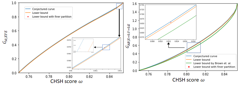
Lemma 2 gives an upper bound on the one-sided randomness using an explicit strategy. However, for security proofs a lower bound is needed. We compute such lower bounds for GA|X​Y​EG_{A|XYE} and GAB|X=0,Y=0,EG_{AB|X=0,Y=0,E}. The relevant computations can be found in Appendices C.2 and C.5.3 (Corollary 4 and Lemma 32) and are displayed in Fig. 2 alongside the upper bounds and a lower bound from Brown et al. 2021b.

The idea is behind our lower bounds is as follows. We first show that for every fixed value of ω\omega the functions GA|X​Y​E​(ω)G_{A|XYE}(\omega) and GAB|X=0,Y=0,E(ω)G_{AB|X=0,Y=0,E}(\omega) can each be expressed as a minimization over 33 real parameters. For fixed ω\omega we compute the values of the objective function on a grid of points comprising these parameters. By bounding the derivative of the objective function within the cuboids generated by the grid we establish a lower bound on the function over the possible parameters. The lower bound we generate can in principle be made arbitrarily good by decreasing the grid spacing (at the expense of taking more time to evaluate).

Given lower bounds on GA|X​Y​E​(ω)G_{A|XYE}(\omega) and GAB|X=0,Y=0,E(ω)G_{AB|X=0,Y=0,E}(\omega) for a finite set of values of ω\omega, we can get lower bounds for all values of ω\omega by using that the GG functions are monotonically increasing in ω\omega, so we have G⁡(ω)≤G⁡(ω−ν)G(\omega)\leq G(\omega-\nu), where ν\nu is the spacing between the finite set of values of ω\omega. Hence, we consider forming lower bounds as above for a set of values 𝒲={ω1,ω2,…}\mathcal{W}=\{\omega_{1},\omega_{2},\ldots\} in the range (3/4,(1/2)​(1+(1/2)1/2)](3/4,(1/2)(1+(1/2)^{1/2})]. We can then consider the points {(ω1,0),(ω2,G⁡(ω1)),(ω3,G⁡(ω2)),…}\{(\omega_{1},0),(\omega_{2},G(\omega_{1})),(\omega_{3},G(\omega_{2})),\ldots\}, i.e., where each is shifted one place. Taking the convex lower bound of these shifted points gives a convex lower bound for GA|X​Y​EG_{A|XYE} and GAB|X=0,Y=0,EG_{AB|X=0,Y=0,E}. By taking more points in the set 𝒲\mathcal{W} tighter lower bounds can be obtained.

Lower bounds generated in this way are shown in Fig. 2, and can be seen to be close to the upper bounds. In Fig. 2(b) we also compare with a lower bound on GAB|X=0,Y=0,EG_{AB|X=0,Y=0,E} from Brown et al. 2021b. The lower bounds from our technique can be improved by refining the partition of the domain at the expense of increasing the computational time required. As seen in Fig. 2(b), refining the partition moves the lower bound closer to the upper bound, leading us to the following conjecture.

Conjecture 1.

The upper bounds in Lemmas 1 and 2 are tight.

One technique for generating finite key rates is to use so-called min-tradeoff functions, which are affine lower bounds on the von Neumann entropy (see Appendix E and Dupuis et al. 2020; Dupuis and Fawzi 2019). Based on an experimental setup, an affine lower bound on GAB|X=0,Y=0,EG_{AB|X=0,Y=0,E} can be generated at the value of ω\omega corresponding to that obtainable in the experiment, hence a refined partition can be used, based only on values of ω\omega close to the experimental value.

Refer to caption

m(a)                          (b)

Figure 2: Graphs of the conjectured rates and lower bounds for (a) GA|X​Y​EG_{A|XYE} (b) GAB|X=0,Y=0,EG_{AB|X=0,Y=0,E} with uniformly chosen inputs. For GAB|X=0,Y=0,EG_{AB|X=0,Y=0,E} we also show a lower bound from Brown et al. Brown et al. 2021b. We also demonstrate that the lower bound for GAB|X=0,Y=0,EG_{AB|X=0,Y=0,E} can be tightened by refining the partitioning of the domain for a specific point (due to the increased computation time, we did not do this throughout).

V Protocols for randomness expansion

In this section we discuss CHSH-based protocols for DIRE of both the spot-checking and non spot-checking types. We pick specific protocols for concreteness, but there are many possible variations. For instance, the protocols we discuss condense the observed statistics to a single score, but this is not necessary, and in some cases and for some sets of experimental conditions it can be advantageous to use multiple scores Brown et al. 2020; Tan et al. 2021.

Before getting to the protocols, we first describe the setup, assumptions and security definition. Although DIRE requires no assumptions on how the devices used operate, the setup for DIRE involves a user who performs the protocol within a secure laboratory, from which information cannot leak. Individual devices can also be isolated within their own sub-laboratory and the user can ensure that these devices only learn the information necessary for the protocol (in particular, they cannot learn any inputs given to other devices). The user has access to a trusted classical computer and an initial source (or sources) of trusted randomness.

The quantum devices used for the protocol are only limited by the laws of quantum theory and may share arbitrary entanglement with each other and with an adversary. However, they cannot communicate with each other, or to the adversary after the protocol starts. Furthermore, we assume they are kept isolated after the protocol (cf. the discussion in Appendix F).

For security of the protocols, we use a composable security definition. Consider a protocol with output ZZ and use Ω\Omega to denote the event that it does not abort. The protocol is (ϵS,ϵC)(\epsilon_{S},\epsilon_{C})-secure if

  1. 1.

    12​pΩ​‖ρZ​E|Ω−1dZ​𝟙ℤ⊗ρ𝔼|Ω‖𝟙≤ϵ𝕊\frac{1}{2}p_{\Omega}||\rho_{ZE|\Omega}-\frac{1}{d_{Z}}\openone_{Z}\otimes\rho_{E|\Omega}||_{1}\leq\epsilon_{S}, where EE represents all the systems held by an adversary and dZd_{Z} is the dimension of system ZZ; and

  2. 2.

    There exists a quantum strategy such that pΩ≥1−ϵCp_{\Omega}\geq 1-\epsilon_{C}.

Here ϵS\epsilon_{S} is called the soundness error, and ϵC\epsilon_{C} is the completeness error.

V.1 CHSH-based spot-checking protocol for randomness expansion

We now describe a spot-checking protocol for randomness expansion. It uses a central biased random number generator RTR_{T} and two other random number generators, RAR_{A} and RBR_{B} that are near each of the devices used to run the protocol.

Protocol 1.

(Spot-checking protocol) a

Parameters:
nn
– number of rounds
γ\gamma – test probability
ωexp\omega_{\exp} – expected CHSH score
δ\delta – confidence width for the score

  1. 1.

    Set i=1i=1 for the first round, or increase ii by 1.

  2. 2.

    Use RTR_{T} to choose Ti∈{0,1}T_{i}\in\{0,1\} where Ti=1T_{i}=1 occurs with probability γ\gamma.

  3. 3.

    If Ti=1T_{i}=1 (test round), RAR_{A} is used to choose XiX_{i} uniformly, which is input to one device giving output AiA_{i}. Likewise RBR_{B} is used to choose YiY_{i} uniformly, which is input to the other device giving output BiB_{i}. Set Ui=1U_{i}=1 if Ai⊕Bi=Xi​YiA_{i}\oplus B_{i}=X_{i}Y_{i} and Ui=0U_{i}=0 otherwise.

  4. 4.

    If Ti=0T_{i}=0 (generation round), the devices are given inputs Xi=Yi=0X_{i}=Y_{i}=0, and return the outputs AiA_{i} and BiB_{i}. Set Ui=⊥U_{i}=\bot.

  5. 5.

    Return to Step 1 unless i=ni=n.

  6. 6.

    Calculate the number of rounds in which Ui=0U_{i}=0 occurred, and abort the protocol if this is larger than n​γ​(1−ωexp+δ)n\gamma(1-\omega_{\exp}+\delta).

  7. 7.

    Process the concatenation of all the outputs with a quantum-proof strong extractor Ext\mathrm{Ext} to yield Ext⁡(𝐀𝐁,𝐑)\mathrm{Ext}({\bf AB},{\bf R}), where 𝐑{\bf R} is a random seed for the extractor. Since a strong extractor is used, the final outcome can be taken to be the concatenation of 𝐑{\bf R} and Ext⁡(𝐀𝐁,𝐑)\mathrm{Ext}({\bf AB},{\bf R}).

There are a few important points to take into account when running the protocol. Firstly, it is crucial that each device only learns its own input and not the value of the other input, or of TiT_{i}. If this is not satisfied it is easy for devices to pass the protocol without generating randomness. Secondly, for implementations in which devices can fail to record outcomes when they should, it is important to close the detection loophole, which can be done by assigning an outcome, say 00, when a device fails to make a detection and otherwise using the same protocol.

In order to run the protocol, some initial randomness is needed to choose which rounds are test rounds, to choose the inputs in the test rounds and to seed the extractor. Since the extractor randomness forms part of the final output, it is not consumed in the protocol, so for considering the rate at which the protocol consumes randomness we can work out the amount of uniform randomness needed to supply the inputs. Using the rounded interval algorithm Hao and Hoshi 1997 to make the biased random number generator, n⁡(Hbin​(γ)+2​γ)+3n(H_{\mathrm{bin}}(\gamma)+2\gamma)+3 is the expected amount of input randomness required. To achieve expansion the number of output bits must be greater than this. We use the entropy accumulation theorem (EAT) to lower bound the amount of output randomness. Asymptotically the relevant quantity is H⁡(A​B|X=0,Y=0,E)H(AB|X=0,Y=0,E). The quantity H⁡(A|X=0,Y=0,E)H(A|X=0,Y=0,E) acts as a lower bound for this, and can be used in its place if convenient, for instance in analyses that are more straightforward with an analytic curve.

V.2 CHSH-based protocols without spot-checking

In this section we discuss two such protocols. Protocol 2 uses two biased local random number generators to choose the inputs on each round. Protocol 3 eliminates the bias, but also recycles the input randomness. Recycling the input randomness is necessary when unbiased random number generators are used, since otherwise more randomness is required to run the protocol than is generated. Protocol 3 gives the highest randomness generation rate of all the protocols we discuss.

Protocol 2.

(Protocol with biased local random number generators) a

Parameters:
nn – number of rounds
ζA\zeta^{A} – probability of 1 for random number generator RAR_{A} (taken to be below 1/21/2)
ζB\zeta^{B} – probability of 1 for random number generator RBR_{B} (taken to be below 1/21/2)
ωexp\omega_{\text{exp}} – expected CHSH score.
δ\delta – confidence widths for each score.

  1. 1.

    Set i=1i=1 for the first round, or increase ii by 1.

  2. 2.

    Use RAR_{A} to choose Xi∈{0,1}X_{i}\in\{0,1\}, which is input to one of the devices giving output Ai∈{0,1}A_{i}\in\{0,1\}. Likewise use RBR_{B} to generate Yi∈{0,1}Y_{i}\in\{0,1\}, which is input to the other device giving output Bi∈{0,1}B_{i}\in\{0,1\}. Here Xi=1X_{i}=1 occurs with probability ζA\zeta^{A} and Yi=1Y_{i}=1 occurs with probability ζB\zeta^{B}. Set Ui=(Xi,Yi,1)U_{i}=(X_{i},Y_{i},1) if Ai⊕Bi=Xi​YiA_{i}\oplus B_{i}=X_{i}Y_{i} and Ui=(Xi,Yi,0)U_{i}=(X_{i},Y_{i},0) otherwise.

  3. 3.

    Return to Step 1 unless i=ni=n.

  4. 4.

    Compute the value

    ω=14∑x,y|{i:Ui=(x,y,1)}|n​pX​(x)​pY​(y)\displaystyle\omega=\frac{1}{4}\sum_{x,y}\frac{|\{i:U_{i}=(x,y,1)\}|}{np_{X}(x)p_{Y}(y)} (4)

    and abort the protocol if ω<ωexp−δ\omega<\omega_{\exp}-\delta. Here pX​(1)=ζAp_{X}(1)=\zeta^{A}, pX​(0)=1−ζAp_{X}(0)=1-\zeta^{A}, pY​(1)=ζBp_{Y}(1)=\zeta^{B} and pY​(0)=1−ζBp_{Y}(0)=1-\zeta^{B}.

  5. 5.

    Process the concatenation of all the outputs with a quantum-proof strong extractor Ext\mathrm{Ext} to yield Ext⁡(𝐀𝐁,𝐑)\mathrm{Ext}({\bf AB},{\bf R}), where 𝐑{\bf R} is a random seed for the extractor. Since a strong extractor is used, the final outcome can be taken to be the concatenation of 𝐑{\bf R} and Ext⁡(𝐀𝐁,𝐑)\mathrm{Ext}({\bf AB},{\bf R}).

Note that the quantity |{i:Ui=(x,y,1)}|/(n​pX​(x)​pY​(y))|\{i:U_{i}=(x,y,1)\}|/(np_{X}(x)p_{Y}(y)) in (4) is an estimate of the probability of winning the CHSH game for inputs X=xX=x and Y=yY=y, and hence the ω\omega computed in Step 4 is an estimate of the CHSH value that would be observed if the same setup was used but with XX and YY chosen uniformly.

The input randomness required per round in this protocol is roughly Hbin​(ζA)+Hbin​(ζB)H_{\mathrm{bin}}(\zeta^{A})+H_{\mathrm{bin}}(\zeta^{B}). To quantify the amount of output randomness (before randomness extraction is performed), in the asymptotic limit similar to the spot checking protocol, the relevant operational quantity is the von Neumann entropy H⁡(A​B|X​Y​E)H(AB|XYE). Expansion hence cannot be achieved if H⁡(A​B|X​Y​E)−Hbin​(ζA)−Hbin​(ζB)<0H(AB|XYE)-H_{\mathrm{bin}}(\zeta^{A})-H_{\mathrm{bin}}(\zeta^{B})<0, which places constraints on the pairs of possible (ζA,ζB)(\zeta^{A},\zeta^{B}). For ζA\zeta^{A} and ζB\zeta^{B} smaller than 1/21/2, the quantity H⁡(A​B|X​Y​E)−Hbin​(ζA)−Hbin​(ζB)H(AB|XYE)-H_{\mathrm{bin}}(\zeta^{A})-H_{\mathrm{bin}}(\zeta^{B}) increases as ζA\zeta^{A} and ζB\zeta^{B} decrease, and hence we want to take these to be small. They only need to be large enough to ensure that X=1,Y=1X=1,Y=1 occurs often enough to give a good estimate of the empirical score.

Since

H⁡(A​B|X​Y​E)\displaystyle H(AB|XYE) =\displaystyle= ∑x​ypX​Y​(x,y)​H​(A​B|X​Y​E)\displaystyle\sum_{xy}p_{XY}(x,y)H(AB|XYE) (5)
≥\displaystyle\geq minx,y⁡H⁡(A​B|X=x,Y=y,E)\displaystyle\min_{x,y}H(AB|X=x,Y=y,E)

we can use the bounds formed for H⁡(A​B|X=0,Y=0,E)H(AB|X=0,Y=0,E) instead77 7 There is nothing special about the choice X=0X=0 and Y=0Y=0 when computing the bounds for H⁡(A​B|X=0,Y=0,E)H(AB|X=0,Y=0,E)., albeit with a loss of entropy (this loss of entropy is small if ζA\zeta_{A} and ζB\zeta_{B} are small).

One reason for using Protocol 2 rather than Protocol 1 is that the former enables the locality loophole to be closed while expanding randomness. In order to perform the Bell tests as part of a device-independent protocol we need to make inputs to two devices in such a way that neither device knows the input of the other. One way to ensure this is by using independent random number generators on each side of the experiment, and ensuring the the outcome of each device is given at space-like separation from the production of the random input to the other. Although space-like separation can provide a guarantee (within the laws of physics) that each device does not know the input of the other88 8 Provided we have a reasonable way to give a time before which the output of RAR_{A} and RBR_{B} did not exist., in a cryptographic setting it is necessary to assume a secure laboratory to prevents any unwanted information leaking from inside the lab to an eavesdropper. The same mechanism by which the lab is shielded from the outside world can be used to shield devices in the lab from one another and hence can prevent communication between the two devices during the protocol. However, although unnecessary for cryptographic purposes, it is interesting to consider closing the locality loophole while expanding randomness.

This is not possible in a typical spot-checking protocol, where a central random number generator is used to decide whether a round is a test round or not. Considering Protocol 1, the locality loophole can be readily closed during the test rounds, but the use of the central random number generator means that, if one is worried that hidden communication channels are being exploited, there is a loophole that the devices could behave differently on test rounds and generation rounds. For instance, measurement devices that know whether a round is a test or generation round could supply pre-programmed outputs in generation rounds, while behaving honestly in test rounds. Thus, spot-checking protocols do not enable fully closing the locality loophole while expanding randomness.

When using Protocol 2 with ζA=ζB=ζ\zeta^{A}=\zeta^{B}=\zeta, the main difference to Protocol 1 is that the distribution of XX and YY is ((1−ζ)2,ζ⁡(1−ζ),ζ⁡(1−ζ),ζ2)((1-\zeta)^{2},\zeta(1-\zeta),\zeta(1-\zeta),\zeta^{2}) rather than (1−3​γ/4,γ/4,γ/4,γ/4)(1-3\gamma/4,\gamma/4,\gamma/4,\gamma/4). In the analysis this manifests itself in the statistics, and the much lower probability of X=1,Y=1X=1,Y=1 requires an adjustment of δ\delta to achieve the same error parameters for the protocol. A comparison between the output rates for Protocols 1 and 2 is shown in Figures 3 and 4.

Protocol 3.

(Protocol with recycled input randomness) a

Parameters:
nn – number of rounds
ωexp\omega_{\exp} – expected CHSH score.
δ\delta – confidence width.

  1. 1.

    Set i=1i=1 for the first round, or increase ii by 1.

  2. 2.

    Use RAR_{A} to choose Xi∈{0,1}X_{i}\in\{0,1\} uniformly, serving as the input to one of the devices giving output Ai∈{0,1}A_{i}\in\{0,1\}. Likewise use RBR_{B} to generate Yi∈{0,1}Y_{i}\in\{0,1\} uniformly, which is input to the other device giving output Bi∈{0,1}B_{i}\in\{0,1\}. Set Ui=1U_{i}=1 if Ai⊕Bi=Xi​YiA_{i}\oplus B_{i}=X_{i}Y_{i} and Ui=0U_{i}=0 otherwise.

  3. 3.

    Return to Step 1 unless i=ni=n.

  4. 4.

    Count the number of rounds for which Ui=0U_{i}=0 occurred and abort the protocol if this is above n⁡(1−ωexp+δ)n(1-\omega_{\exp}+\delta).

  5. 5.

    Process the concatenation of all the inputs and outputs with a quantum-proof strong extractor Ext\mathrm{Ext} to yield Ext⁡(𝐀𝐁𝐗𝐘,𝐑)\mathrm{Ext}({\bf ABXY},{\bf R}), where 𝐑{\bf R} is a random seed for the extractor. Since a strong extractor is used, the final outcome can be taken to be the concatenation of 𝐑{\bf R} and Ext⁡(𝐀𝐁𝐗𝐘,𝐑)\mathrm{Ext}({\bf ABXY},{\bf R}).

An important difference in this protocol compared to Protocols 1 and 2 is in the extraction step, which now extracts randomness from the input strings 𝐗{\bf X} and 𝐘{\bf Y} as well as the outputs. Without recycling the inputs expansion would not be possible in Protocol 3. With the modification the relevant quantity to decide the length of the output is H⁡(A​B​X​Y|E)H(ABXY|E), and so H⁡(A​B|X​Y​E)=H⁡(A​B​X​Y|E)−H⁡(X​Y)=H⁡(A​B​X​Y|E)−2H(AB|XYE)=H(ABXY|E)-H(XY)=H(ABXY|E)-2 is the relevant quantity for calculating the rate of expansion. Note that in order to reuse the input in a composable way, it also needs to be run through an extractor Colbeck and Kent 2011 (for a discussion of why it is important to do so and a few more composability-related issues, see Appendix F).

We could also consider an adaptation of Protocol 1 in which the input randomness is recycled, forming Protocol 1′ from Protocol 1 by replacing Step 7 by

  1. 7′.

    Process the concatenation of all the inputs and outputs with a quantum-proof strong extractor Ext\mathrm{Ext} to yield Ext⁡(𝐀𝐁𝐗𝐘,𝐑)\mathrm{Ext}({\bf ABXY},{\bf R}), where 𝐑{\bf R} is a random seed for the extractor. Since a strong extractor is used, the final outcome can be taken to be the concatenation of 𝐑{\bf R} and Ext⁡(𝐀𝐁𝐗𝐘,𝐑)\mathrm{Ext}({\bf ABXY},{\bf R}).

In this case, as the number of rounds, nn, increases the advantage gained by this modification decreases, becoming negligible asymptotically. This is because as nn increases, the value of γ\gamma required to give the same overall security tends to zero, and hence the amount of input randomness required becomes negligible. Note that recycling the input randomness in Protocol 2 in the case where ζA=ζB=1/2\zeta^{A}=\zeta^{B}=1/2 is equivalent to Protocol 3.

Like Protocol 2, Protocol 3 also allows the locality loophole to be closed if on each round ii, the random choice XiX_{i} is space-like separated from the output BiB_{i} and the random choice YiY_{i} is space-like separated from the output AiA_{i}.

Refer to caption

m(a)                (b)                (c)

Figure 3: Graphs of the net rate of certifiable randomness according to the EAT for (a) the spot checking protocol (Protocol 1), (b) the protocol with recycled input randomness (Protocol 3), and (c) the protocol with biased local random number generators (Protocol 2), showing the variation with the number of rounds for three different scores, ω\omega. The error parameters used were ϵS=3.09×10⁻¹²\epsilon_{S}=3.09\times 10^{-12} and ϵC=10−6\epsilon_{C}=10^{-6}. For each point on the curve (a) an optimization over γ\gamma was performed to maximize the randomness; similarly, the values of ζA=ζB\zeta^{A}=\zeta^{B} were optimized over to generate the curves in (c).
Refer to caption

m(a)                (b)                (c)

Figure 4: Graphs of the net rate of certifiable randomness according to the EAT for (a) the spot checking protocol (Protocol 1), (b) the protocol with recycled input randomness (Protocol 3), and (c) the protocol with biased local random number generators (Protocol 2), showing the variation with the CHSH score ω\omega. The round numbers, nn, are indicated in the legend. The error parameters used were ϵS=3.09×10⁻¹²\epsilon_{S}=3.09\times 10^{-12} and ϵC=10−6\epsilon_{C}=10^{-6}. As in Figure 3, the values of γ\gamma (for (a)) and ζA=ζB\zeta^{A}=\zeta^{B} (for (c)) were optimized over for each point.

In each of the protocols, the parameter δ\delta should be chosen depending on the desired completeness error. For the spot-checking protocol, the relation between the two is discussed in (Liu et al. 2021, Supplementary Information I D). The analysis there can be applied to the protocol with recycled input randomness by setting γ=1\gamma=1 and the protocol with biased local random number generators is discussed in Appendix E.3.2. The chosen soundness error affects the length of the extractor output, and, if chosen too small the output length becomes zero (see Appendix E for further discussion).

Figures 3 and 4 show how the amount of certifiable randomness varies with the score, ω\omega, and round number, nn. Note that in the cases where the rate curves of Figure 1 have linear sections, they are linear for most of their ranges. Extending the linear part to the full range of quantum scores makes it easier to use the EAT while only resulting in a small drop in rate for scores close to the maximum quantum value. Note that, as mentioned above, strictly the numerical curves we gave for the von Neumann entropy are upper bounds; the curves in Figures 3 and 4 are generated under the assumption that these upper bounds are tight. [In the case of the spot-checking protocol (Protocol 1) we could use our lower bound instead. This would result in a small down-shifting of the curves, but mean that the bounds are provably reliable.]

To demonstrate the increased practicality of the two-sided curves, we use the parameters from a recent experiment Liu et al. 2021 with Protocol 1. There a score of just over 0.7520.752 was obtained, for which it would require about 9×10109\times 10^{10} rounds to achieve expansion using Protocol 1 with γ=3.383×10⁻⁴\gamma=3.383\times 10^{-4}, ϵS=3.09×10⁻¹²\epsilon_{S}=3.09\times 10^{-12}, ϵC=10−6\epsilon_{C}=10^{-6} and taking the one-sided randomness Liu et al. 2021. Using Protocol 3 instead, and taking the two-sided randomness for the same score and error parameters (assuming Conjecture 1 holds) allows expansion for n≳8×10⁷n\gtrsim 8\times 10^{7}, significantly increasing the practicality. For instance, the main experiment of Liu et al. 2021 was based on a spot-checking protocol and took 19.219.2 hours; the use of Protocol 3 instead would allow the same amount of expansion in about 6060 seconds (this time holds under the assumption that the same repetition rate of the experiment can be met in the non-spot checking protocol99 9 In some experiments, the rate at which we can switch between the two measurements is relatively slow, and hence when using Protocol 3, where switching is required on most rounds, the switching rate dominates, slightly increasing the time.). Protocol 2, however, produces lower randomness rates compared to the spot-checking protocol. This is partly because more input randomness is required, and also because the completeness error has a worse behaviour. Protocol 2 is hence useful when inputs are not recycled and when closing the locality loophole is desirable.

When discussing randomness expansion we have considered the figure of merit to be the amount of expansion per entangled pair shared. An alternative figure of merit is the ratio of the final randomness to the initial randomness, i.e., here we are considering how much randomness we can get from a given amount of initial randomness. For the latter figure of merit, Protocol 3 is no longer optimal, since the amount of expansion cannot exceed the amount of input randomness. For the other two protocols the ratio of output randomness to input randomness can be made much higher by taking either γ\gamma or ζA​ζB\zeta^{A}\zeta^{B} to be small.

VI Discussion

In this paper, we have given numerical bounds on various conditional von Neumann entropies that are relevant for CHSH-based device-independent protocols and discussed when each can be applied. We have investigated their implications using explicit protocols, comparing the finite statistics rates using the EAT, showing use of two-sided randomness has the potential to make a big difference. We also looked at protocols beyond the usual spot checking type. The first removes the spot checking to allow expansion while closing the locality loophole, and the second recycles the input randomness, so allowing expansion while performing a CHSH test on every round.

It remains an open question to find an analytic form for FAB|X=0,Y=0,EF_{AB|X=0,Y=0,E}, FA|EF_{A|E} and FA​B|EF_{AB|E}. Since the curves FA|EF_{A|E} and FA​B|EF_{AB|E} are linear for all but the very highest (experimentally least achievable) scores, in these cases not much is lost by extending the line to all scores forming a lower bound that tightly covers all of the experimentally relevant cases. On the other hand FAB|X=0,Y=0,EF_{AB|X=0,Y=0,E} is a convex curve throughout and hence a tight analytic form would be particularly useful in this case. Our initial analysis suggests that form of the parameters achieving the optima for these is sufficiently complicated that any analytic expression would not be compact. A reasonably tight analytic lower bound for FAB|X=0,Y=0,EF_{AB|X=0,Y=0,E} could also be useful for theoretical analysis. Note also that the bound FA|E≥FA|X​Y​EF_{A|E}\geq F_{A|XYE} appears to be fairly tight (see Figure 1(a)) so the analytic form for FA|X​Y​EF_{A|XYE} can be used to bound FA|EF_{A|E} with little loss. Another open problem is to find a concrete scenario in which FA​B|EF_{AB|E} is directly useful.

The use of Jordan’s lemma in this work prevents the techniques used being extended to general protocols, and finding improved ways to bound the conditional von Neumann entropy numerically in general cases remains of interest. For example, protocols that use three inputs for one party can allow up to 2 bits of randomness per entangled pair (see, e.g. Brown et al. 2020), and a way to tightly lower bound the von Neumann entropy in this case would further ease the experimental burden required to demonstrate DIQKD in the lab.

Additional note: While completing this work a new paper appeared Tan et al. 2022, which also found numerical curves for H⁡(A|X​Y​E)H(A|XYE) and used them with some new protocols to generate improved rates for DIQKD.

Acknowledgements.
We thank Erik Woodhead for useful comments and Peter Brown for sharing his data used in Figure 2. This work was supported by the Quantum Communications Hub of the UK Engineering and Physical Sciences Research Council (EPSRC) (grant nos. EP/M013472/1 and EP/T001011/1).

Appendix A Additional graphs

Figure 5(a) gives the graphs of FA​B|X​Y​E​(ω)F_{AB|XYE}(\omega) and GA​B|X​Y​E​(ω)G_{AB|XYE}(\omega), while Figure 5(b) shows those for FA|X​Y​E​(ω)F_{A|XYE}(\omega) and GA|X​Y​E​(ω)G_{A|XYE}(\omega). In each case the GG graphs have a concave and convex part and the FF graphs are formed by taking the convex lower bound. For these cases the points at which the tangents are taken are ωA​B|X​Y​E∗≈0.8440\omega^{*}_{AB|XYE}\approx 0.8440 and ωA|X​Y​E∗≈0.8470\omega^{*}_{A|XYE}\approx 0.8470.

Figure 6(a) gives the graphs of FA​B|E​(ω)F_{AB|E}(\omega) and GA​B|E​(ω)G_{AB|E}(\omega), while Figure 6(b) shows those for FA|X​Y​E​(ω)F_{A|XYE}(\omega) and GA|X​Y​E​(ω)G_{A|XYE}(\omega). Again, in each case the GG graphs have a concave and convex part and the FF graphs are formed by taking the convex lower bound. For these cases the points at which the tangents are taken are ωA|E∗≈0.8505\omega^{*}_{A|E}\approx 0.8505 and ωA​B|E∗≈0.8523\omega^{*}_{AB|E}\approx 0.8523.

Refer to caption

(a)                        (b)

Figure 5: (a) Two-sided and (b) one-sided entropy curves conditioned on XX, YY and EE with uniform input distribution.
Refer to caption

(a)                        (b)

Figure 6: (a) Two-sided and (b) one-sided entropy curves conditioned on EE with uniform input distribution.

Appendix B Simplifying the strategy

Given a Hilbert space ℋ\mathcal{H}, we use 𝒫⁡(ℋ)\mathcal{P}(\mathcal{H}) to be the set of positive semi-definite operators on ℋ\mathcal{H}, and 𝒮⁡(ℋ)\mathcal{S}(\mathcal{H}) to be the set of density operators, i.e., elements of 𝒫\mathcal{P} with trace 1. The pure states on ℋ\mathcal{H} (elements of 𝒮⁡(ℋ)\mathcal{S}(\mathcal{H}) with rank 1) will be denoted 𝒮P​(ℋ)\mathcal{S}_{P}(\mathcal{H}). A POVM on ℋ\mathcal{H} is a set of positive operators {Ei}i\{E_{i}\}_{i} with Ei∈𝒫⁡(ℋ)E_{i}\in\mathcal{P}(\mathcal{H}) for all ii and ∑iEi=𝟙ℋ\sum_{i}E_{i}=\openone_{\mathcal{H}}, where 𝟙ℋ\openone_{\mathcal{H}} is the identity operator on ℋ\mathcal{H}. A projective measurement on ℋ\mathcal{H} is a POVM on ℋ\mathcal{H} where Ei2=EiE_{i}^{2}=E_{i} for all ii. We define the Bell states

|Φ0⟩\displaystyle|\Phi_{0}\rangle =\displaystyle= 12​(|00⟩+|11⟩)\displaystyle\frac{1}{\sqrt{2}}\left(|00\rangle+|11\rangle\right) (6)
|Φ1⟩\displaystyle|\Phi_{1}\rangle =\displaystyle= 12​(|00⟩−|11⟩)\displaystyle\frac{1}{\sqrt{2}}\left(|00\rangle-|11\rangle\right) (7)
|Φ2⟩\displaystyle|\Phi_{2}\rangle =\displaystyle= 12​(|01⟩+|10⟩)\displaystyle\frac{1}{\sqrt{2}}\left(|01\rangle+|10\rangle\right) (8)
|Φ3⟩\displaystyle|\Phi_{3}\rangle =\displaystyle= 12​(|01⟩−|10⟩),\displaystyle\frac{1}{\sqrt{2}}\left(|01\rangle-|10\rangle\right)\,, (9)

and use σ1=|1⟩​⟨0|+|0⟩​⟨1|\sigma_{1}=|1\rangle\!\langle 0|+|0\rangle\!\langle 1|, σ2=i⁡|1⟩​⟨0|−i|0⟩​⟨1|\sigma_{2}=\mathrm{i}|1\rangle\!\langle 0|-\mathrm{i}|0\rangle\!\langle 1| and σ3=|0⟩​⟨0|−|1⟩​⟨1|\sigma_{3}=|0\rangle\!\langle 0|-|1\rangle\!\langle 1| as the three Pauli operators.

In this section we make a series of simplifications of the form of the optimization. The argument given broadly follows the logic of Pironio et al. 2009 (see also Woodhead et al. 2021 for an alternative).

Definition 1.

A single-round CHSH measurement strategy is a tuple (ℋA′,ℋB′,{Ma|x}x,a,{Nb|y}y,b)(\mathcal{H}_{A^{\prime}},\mathcal{H}_{B^{\prime}},\{M_{a|x}\}_{x,a},\{N_{b|y}\}_{y,b}), where ℋA′\mathcal{H}_{A^{\prime}} and ℋB′\mathcal{H}_{B^{\prime}} are Hilbert spaces, and {Ma|x}a\{M_{a|x}\}_{a} is a POVM on ℋA′\mathcal{H}_{A^{\prime}} for each x∈{0,1}x\in\{0,1\} and likewise {Nb|y}b\{N_{b|y}\}_{b} is a POVM on ℋB′\mathcal{H}_{B^{\prime}} for each y∈{0,1}y\in\{0,1\}. In the case that all the POVMs are projective we will call this a single-round CHSH projective measurement strategy.

Definition 2.

A single-round CHSH strategy is a single-round CHSH measurement strategy together with a state ρA′​B′​E∈ℋA′⊗ℋB′⊗ℋE\rho_{A^{\prime}B^{\prime}E}\in\mathcal{H}_{A^{\prime}}\otimes\mathcal{H}_{B^{\prime}}\otimes\mathcal{H}_{E}, where ℋE\mathcal{H}_{E} is an arbitrary Hilbert space.

Note that in a device-independent scenario, such a strategy can be chosen by the adversary.

Definition 3.

Given a single-round CHSH measurement strategy and a distribution pX​Yp_{XY} over the settings XX and YY, the associated CHSH channel is defined by

𝒩:𝒮⁡(ℋA′⊗ℋB′)→𝒮⁡(ℋA⊗ℋB⊗ℋX⊗ℋY):σ↦∑a​b​x​ypX​Y​(x,y)​|a⟩​⟨a|⊗|b⟩​⟨b|⊗|x⟩​⟨x|⊗|y⟩​⟨y|​tr​((Ma|x⊗Nb|y)​σ),\mathcal{N}:\mathcal{S}(\mathcal{H}_{A^{\prime}}\otimes\mathcal{H}_{B^{\prime}})\to\mathcal{S}(\mathcal{H}_{A}\otimes\mathcal{H}_{B}\otimes\mathcal{H}_{X}\otimes\mathcal{H}_{Y}):\sigma\mapsto\sum_{abxy}p_{XY}(x,y)|a\rangle\!\langle a|\otimes|b\rangle\!\langle b|\otimes|x\rangle\!\langle x|\otimes|y\rangle\!\langle y|\mathrm{tr}\left((M_{a|x}\otimes N_{b|y})\sigma\right)\,,

where ℋA\mathcal{H}_{A}, ℋB\mathcal{H}_{B}, ℋX\mathcal{H}_{X} and ℋY\mathcal{H}_{Y} are two dimensional Hilbert spaces. The union of the sets of associated CHSH channels for all single-round CHSH measurement strategies for some fixed input distribution pX​Yp_{XY} is denoted 𝒞⁡(pX​Y)\mathcal{C}(p_{XY}). The union of the sets of associated CHSH channels for all single-round CHSH projective measurement strategies is denoted 𝒞Π​(pX​Y)\mathcal{C}_{\Pi}(p_{XY}).

The output of the associated CHSH channel is classical, and ℋA⊗ℋB⊗ℋX⊗ℋY\mathcal{H}_{A}\otimes\mathcal{H}_{B}\otimes\mathcal{H}_{X}\otimes\mathcal{H}_{Y} stores the outcomes and the chosen measurements. We will usually apply this channel to the A​BAB part of a tripartite system, giving

(𝒩⊗ℐE)​(ρA′​B′​E)=∑a​b​x​ypX​Y​(x,y)​pA​B|x​y​(a,b)​|a⟩​⟨a|⊗|b⟩​⟨b|⊗|x⟩​⟨x|⊗|y⟩​⟨y|⊗τEa,b,x,y,(\mathcal{N}\otimes\mathcal{I}_{E})(\rho_{A^{\prime}B^{\prime}E})=\sum_{abxy}p_{XY}(x,y)p_{AB|xy}(a,b)|a\rangle\!\langle a|\otimes|b\rangle\!\langle b|\otimes|x\rangle\!\langle x|\otimes|y\rangle\!\langle y|\otimes\tau^{a,b,x,y}_{E}\,, (10)

where τEa,b,x,y∈𝒮⁡(ℋE)\tau^{a,b,x,y}_{E}\in\mathcal{S}(\mathcal{H}_{E}) for each a,b,x,ya,b,x,y (it is the normalization of trA′​B′​((Ma|x⊗Nb|y⊗𝟙𝔼)​ρ𝔸′​𝔹′​𝔼)\mathrm{tr}_{A^{\prime}B^{\prime}}\left((M_{a|x}\otimes N_{b|y}\otimes\openone_{E})\rho_{A^{\prime}B^{\prime}E}\right)).

Note that the CHSH score, which we denote S⁡((𝒩⊗ℐE)​(ρA′​B′​E))S((\mathcal{N}\otimes\mathcal{I}_{E})(\rho_{A^{\prime}B^{\prime}E})) does not depend on the distribution pX​Yp_{XY} of input settings.

We will be interested in optimization problems of the form

F⁡(ω,pX​Y)=\displaystyle F(\omega,p_{XY})= infℛH¯​((𝒩⊗ℐE)​(ρA′​B′​E))​ where\displaystyle\inf_{\mathcal{R}}\bar{H}((\mathcal{N}\otimes\mathcal{I}_{E})(\rho_{A^{\prime}B^{\prime}E}))\text{ where } (11)
ℛ={(𝒩,ρA′​B′​E):𝒩∈𝒞(pX​Y),S((𝒩⊗ℐE)(ρA′​B′​E))=ω}\displaystyle\mathcal{R}=\{(\mathcal{N},\rho_{A^{\prime}B^{\prime}E}):\mathcal{N}\in\mathcal{C}(p_{XY}),\,S((\mathcal{N}\otimes\mathcal{I}_{E})(\rho_{A^{\prime}B^{\prime}E}))=\omega\}

where ℋE\mathcal{H}_{E} is an arbitrary Hilbert space and the spaces ℋA′\mathcal{H}_{A^{\prime}} and ℋB′\mathcal{H}_{B^{\prime}} are those from the chosen element of 𝒞⁡(pX​Y)\mathcal{C}(p_{XY}), i.e., the set ℛ⁡(ω)\mathcal{R}(\omega) runs over all possible dimensions of these spaces, and ω\omega is some fixed real number. Here H¯\bar{H} can be any one of the following entropic quantities defined on the state (𝒩⊗ℐE)​(ρA′​B′​E)(\mathcal{N}\otimes\mathcal{I}_{E})(\rho_{A^{\prime}B^{\prime}E}): H⁡(A​B|X=0,Y=0,E)H(AB|X=0,Y=0,E), H⁡(A​B|X​Y​E)H(AB|XYE), H⁡(A​B|E)H(AB|E), H⁡(A|X=0,Y=0,E)H(A|X=0,Y=0,E), H⁡(A|X​Y​E)H(A|XYE) or H⁡(A|E)H(A|E). We consider the family of optimizations in this work and many of the arguments that follow are independent of this choice.

B.1 Reduction to projective measurements

In this section, we conclude that there is no loss in generality in assuming that the devices perform projective measurements. More precisely, we prove the following lemma.

Lemma 3.

The sets

𝒯1\displaystyle\mathcal{T}_{1} :⁣=\displaystyle:= {(𝒩⊗ℐE)(ρA′​B′​E):𝒩∈𝒞(pX​Y),ρA′​B′​E∈𝒮(ℋA′⊗ℋB′⊗ℋE)} and\displaystyle\{(\mathcal{N}\otimes\mathcal{I}_{E})(\rho_{A^{\prime}B^{\prime}E}):\mathcal{N}\in\mathcal{C}(p_{XY}),\rho_{A^{\prime}B^{\prime}E}\in\mathcal{S}(\mathcal{H}_{A^{\prime}}\otimes\mathcal{H}_{B^{\prime}}\otimes\mathcal{H}_{E})\}\text{ and}
𝒯2\displaystyle\mathcal{T}_{2} :⁣=\displaystyle:= {(𝒩⊗ℐE)(ρA′​B′​E):𝒩∈𝒞Π(pX​Y),ρA′​B′​E∈𝒮(ℋA′⊗ℋB′⊗ℋE)}\displaystyle\{(\mathcal{N}\otimes\mathcal{I}_{E})(\rho_{A^{\prime}B^{\prime}E}):\mathcal{N}\in\mathcal{C}_{\Pi}(p_{XY}),\rho_{A^{\prime}B^{\prime}E}\in\mathcal{S}(\mathcal{H}_{A^{\prime}}\otimes\mathcal{H}_{B^{\prime}}\otimes\mathcal{H}_{E})\}

are identical.

This is a corollary of Naimark’s theorem, which we state in the following way.

Theorem 1 (Naimark’s theorem).

Let {Ei}i\{E_{i}\}_{i} be a POVM on ℋ\mathcal{H}. There exists a Hilbert space ℋ′\mathcal{H}^{\prime} and a projective measurement {Πi}i\{\Pi_{i}\}_{i} on ℋ⊗ℋ′\mathcal{H}\otimes\mathcal{H}^{\prime} such that for any ρ∈𝒮⁡(ℋ)\rho\in\mathcal{S}(\mathcal{H})

∑i|i⟩​⟨i|​tr​(ρ​Ei)=∑i|i⟩​⟨i|​tr​(Πi​(ρ⊗|0⟩​⟨0|)).\sum_{i}|i\rangle\!\langle i|\mathrm{tr}(\rho E_{i})=\sum_{i}|i\rangle\!\langle i|\mathrm{tr}(\Pi_{i}(\rho\otimes|0\rangle\!\langle 0|))\,.
Proof.

We can directly construct this measurement as follows. Consider the isometry V:ℋ→ℋ⊗ℋ′V:\mathcal{H}\to\mathcal{H}\otimes\mathcal{H}^{\prime} given by V=∑iEi⊗|i⟩V=\sum_{i}\sqrt{E_{i}}\otimes|i\rangle, and let UU be the extension of VV to a unitary with the property that U⁡(|ψ⟩⊗|0⟩)=∑iEi​|ψ⟩⊗|i⟩U(|\psi\rangle\otimes|0\rangle)=\sum_{i}\sqrt{E_{i}}|\psi\rangle\otimes|i\rangle for any |ψ⟩∈ℋ|\psi\rangle\in\mathcal{H}. This construction ensures that the channels

ℰ:ρ\displaystyle\mathcal{E}:\rho ↦\displaystyle\mapsto ∑i|i⟩​⟨i|​tr​(Ei​ρ)​ and\displaystyle\sum_{i}|i\rangle\!\langle i|\mathrm{tr}(E_{i}\rho)\text{ and}
ℰ′:ρ\displaystyle\mathcal{E}^{\prime}:\rho ↦\displaystyle\mapsto ∑i|i⟩​⟨i|​tr​((𝟙⊗|𝕚⟩​⟨𝕚|)​𝕌​(ρ⊗|𝟘⟩​⟨𝟘|)​𝕌†)\displaystyle\sum_{i}|i\rangle\!\langle i|\mathrm{tr}\left((\openone\otimes|i\rangle\!\langle i|)U(\rho\otimes|0\rangle\!\langle 0|)U^{\dagger}\right)

are identical. The second of these can be rewritten

ρ↦∑i|i⟩​⟨i|​tr​(Πi​(ρ⊗|0⟩​⟨0|)),\rho\mapsto\sum_{i}|i\rangle\!\langle i|\mathrm{tr}\left(\Pi_{i}(\rho\otimes|0\rangle\!\langle 0|)\right)\,,

where we take Πi=U†​(𝟙⊗|𝕚⟩​⟨𝕚|)​𝕌\Pi_{i}=U^{\dagger}(\openone\otimes|i\rangle\!\langle i|)U, as required. ∎

Proof of Lemma 3.

By definition 𝒯2⊆𝒯1\mathcal{T}_{2}\subseteq\mathcal{T}_{1}. For the other direction, consider a state ρA′​B′​E\rho_{A^{\prime}B^{\prime}E} and POVMs {Ma|x}a,x\{M_{a|x}\}_{a,x} and {Nb|y}b,y\{N_{b|y}\}_{b,y} forming a single-round CHSH strategy in 𝒯1\mathcal{T}_{1}. We use the construction in the proof of Theorem 1 to generate the projectors Πa|xA\Pi^{A}_{a|x} and Πb|yB\Pi^{B}_{b|y} as Naimark extensions of the POVMs. Instead of creating the state ρA′​B′​E\rho_{A^{\prime}B^{\prime}E}, the state ρA′​B′​E⊗|0⟩​⟨0|A′′⊗|0⟩​⟨0|B′′\rho_{A^{\prime}B^{\prime}E}\otimes|0\rangle\!\langle 0|_{A^{\prime\prime}}\otimes|0\rangle\!\langle 0|_{B^{\prime\prime}} is created instead, where the projectors Πa|xA\Pi^{A}_{a|x} act on A′​A′′A^{\prime}A^{\prime\prime} and Πb|yB\Pi^{B}_{b|y} act on B′​B′′B^{\prime}B^{\prime\prime}. Since the latter is a strategy in 𝒯2\mathcal{T}_{2} leading to the same post-measurement state (10), we have 𝒯1⊆𝒯2\mathcal{T}_{1}\subseteq\mathcal{T}_{2}, which completes the proof. ∎

B.2 Reduction to convex combinations of qubit strategies

This is a consequence of Jordan’s lemma Jordan 1875 and is a special feature that applies only because the Bell inequality has two inputs and two outputs for each party.

Lemma 4 (Jordan’s lemma).

Let A1A_{1} and A2A_{2} be two Hermitian operators on ℋ\mathcal{H} with eigenvalues ±1\pm 1, then we can decompose ℋ=⨁αℋα\mathcal{H}=\bigoplus_{\alpha}\mathcal{H}_{\alpha} such that A1A_{1} and A2A_{2} preserve the subspaces ℋα\mathcal{H}_{\alpha}, and where each ℋα\mathcal{H}_{\alpha} has dimension at most 2.

Corollary 1.

Let Π1\Pi_{1} and Π2\Pi_{2} be two projections on ℋ\mathcal{H}. We can decompose ℋ=⨁αℋα\mathcal{H}=\bigoplus_{\alpha}\mathcal{H}_{\alpha} such that Π1\Pi_{1}, 𝟙−Π𝟙\openone-\Pi_{1}, Π2\Pi_{2} and 𝟙−Π𝟚\openone-\Pi_{2} preserve the subspaces ℋα\mathcal{H}_{\alpha}, and where each ℋα\mathcal{H}_{\alpha} has dimension at most 2.

Proof.

Apply Jordan’s lemma to the Hermitian operators A1=2​Π1−𝟙A_{1}=2\Pi_{1}-\openone and A2=2​Π2−𝟙A_{2}=2\Pi_{2}-\openone with eigenvalues ±1\pm 1, and consider |ψ⟩∈ℋα|\psi\rangle\in\mathcal{H}_{\alpha} for some α\alpha. By construction A1​|ψ⟩∈ℋαA_{1}|\psi\rangle\in\mathcal{H}_{\alpha} from which it follows that Π1​|ψ⟩∈ℋα\Pi_{1}|\psi\rangle\in\mathcal{H}_{\alpha}, and hence also (𝟙−Π𝟙)​|ψ⟩∈ℋα(\openone-\Pi_{1})|\psi\rangle\in\mathcal{H}_{\alpha}. Thus, Π1\Pi_{1} and 𝟙−Π𝟙\openone-\Pi_{1} preserve the subspace; likewise Π2\Pi_{2} and 𝟙−Π𝟚\openone-\Pi_{2}. ∎

This implies the following

Lemma 5.

Let 𝒞2×2​(pX​Y)\mathcal{C}_{2\times 2}(p_{XY}) be the set of CHSH channels associated with the single-round CHSH projective measurement strategies where each of the four projectors Ma|xM_{a|x} is block diagonal with 2×22\times 2 blocks, and each of the four projectors Nb|yN_{b|y} is block diagonal with 2×22\times 2 blocks. The sets

𝒯2\displaystyle\mathcal{T}_{2} :⁣=\displaystyle:= {(𝒩⊗ℐE)(ρA′​B′​E):𝒩∈𝒞Π(pX​Y),ρA′​B′​E∈𝒮(ℋA′⊗ℋB′⊗ℋE)} and\displaystyle\{(\mathcal{N}\otimes\mathcal{I}_{E})(\rho_{A^{\prime}B^{\prime}E}):\mathcal{N}\in\mathcal{C}_{\Pi}(p_{XY}),\rho_{A^{\prime}B^{\prime}E}\in\mathcal{S}(\mathcal{H}_{A^{\prime}}\otimes\mathcal{H}_{B^{\prime}}\otimes\mathcal{H}_{E})\}\text{ and}
𝒯3\displaystyle\mathcal{T}_{3} :⁣=\displaystyle:= {(𝒩⊗ℐE)(ρA′​B′​E):𝒩∈𝒞2×2(pX​Y),ρA′​B′​E∈𝒮(ℋA′⊗ℋB′⊗ℋE)}\displaystyle\{(\mathcal{N}\otimes\mathcal{I}_{E})(\rho_{A^{\prime}B^{\prime}E}):\mathcal{N}\in\mathcal{C}_{2\times 2}(p_{XY}),\rho_{A^{\prime}B^{\prime}E}\in\mathcal{S}(\mathcal{H}_{A^{\prime}}\otimes\mathcal{H}_{B^{\prime}}\otimes\mathcal{H}_{E})\}

are identical.

Proof.

This follows by applying Corollary 1 to the projectors M0|0M_{0|0} and M0|1M_{0|1} to get the blocks on ℋA′\mathcal{H}_{A^{\prime}} and to the projectors N0|0N_{0|0} and N0|1N_{0|1} to get the blocks on ℋB′\mathcal{H}_{B^{\prime}}. Although some of the blocks may be 1×11\times 1, we can collect these together and treat them as a 2×22\times 2 block, or add an extra dimension to the space (on which the state has no support) to achieve all 2×22\times 2 blocks. ∎

We can also make the state only have support on the 2×22\times 2 blocks.

Lemma 6.

The sets

𝒯3\displaystyle\mathcal{T}_{3} :⁣=\displaystyle:= {(𝒩⊗ℐE)(ρA′​B′​E):𝒩∈𝒞2×2(pX​Y),ρA′​B′​E∈𝒮(ℋA′⊗ℋB′⊗ℋE)} and\displaystyle\{(\mathcal{N}\otimes\mathcal{I}_{E})(\rho_{A^{\prime}B^{\prime}E}):\mathcal{N}\in\mathcal{C}_{2\times 2}(p_{XY}),\rho_{A^{\prime}B^{\prime}E}\in\mathcal{S}(\mathcal{H}_{A^{\prime}}\otimes\mathcal{H}_{B^{\prime}}\otimes\mathcal{H}_{E})\}\text{ and}
𝒯4\displaystyle\mathcal{T}_{4} :⁣=\displaystyle:= {(𝒩⊗ℐE)(ρA′​B′​E):𝒩∈𝒞2×2(pX​Y),ρA′​B′​E∈𝒮2×2(ℋA′⊗ℋB′⊗ℋE)}\displaystyle\{(\mathcal{N}\otimes\mathcal{I}_{E})(\rho_{A^{\prime}B^{\prime}E}):\mathcal{N}\in\mathcal{C}_{2\times 2}(p_{XY}),\rho_{A^{\prime}B^{\prime}E}\in\mathcal{S}_{2\times 2}(\mathcal{H}_{A^{\prime}}\otimes\mathcal{H}_{B^{\prime}}\otimes\mathcal{H}_{E})\}

are identical. Here 𝒮2×2​(ℋA′⊗ℋB′⊗ℋE)\mathcal{S}_{2\times 2}(\mathcal{H}_{A^{\prime}}\otimes\mathcal{H}_{B^{\prime}}\otimes\mathcal{H}_{E}) is the subset of 𝒮⁡(ℋA′⊗ℋB′⊗ℋE)\mathcal{S}(\mathcal{H}_{A^{\prime}}\otimes\mathcal{H}_{B^{\prime}}\otimes\mathcal{H}_{E}) such that ρA′​B′​E∈𝒮2×2​(ℋA′⊗ℋB′⊗ℋE)\rho_{A^{\prime}B^{\prime}E}\in\mathcal{S}_{2\times 2}(\mathcal{H}_{A^{\prime}}\otimes\mathcal{H}_{B^{\prime}}\otimes\mathcal{H}_{E}) implies

ρA′​B′​E=∑α,β(ΠA′α⊗ΠB′β⊗𝟙𝔼)​ρ𝔸′​𝔹′​𝔼​(Π𝔸′α⊗Π𝔹′β⊗𝟙𝔼),\rho_{A^{\prime}B^{\prime}E}=\sum_{\alpha,\beta}(\Pi^{\alpha}_{A^{\prime}}\otimes\Pi^{\beta}_{B^{\prime}}\otimes\openone_{E})\rho_{A^{\prime}B^{\prime}E}(\Pi^{\alpha}_{A^{\prime}}\otimes\Pi^{\beta}_{B^{\prime}}\otimes\openone_{E})\,,

where {Πα}α\{\Pi^{\alpha}\}_{\alpha} are projectors onto the 2×22\times 2 diagonal blocks.

Proof.

Consider a state ρA′​B′​E\rho_{A^{\prime}B^{\prime}E} and sets of projectors {Ma|x}a,x\{M_{a|x}\}_{a,x} and {Nb|y}b,y\{N_{b|y}\}_{b,y} from the set 𝒯3\mathcal{T}_{3}. For brevity, write Πα,β=ΠA′α⊗ΠB′β\Pi^{\alpha,\beta}=\Pi^{\alpha}_{A^{\prime}}\otimes\Pi^{\beta}_{B^{\prime}}. Then, since

Ma|x⊗Nb|y=∑α,β(ΠA′α⊗ΠB′β)​(Ma|x⊗Nb|y)​(ΠA′α⊗ΠB′β),M_{a|x}\otimes N_{b|y}=\sum_{\alpha,\beta}(\Pi^{\alpha}_{A^{\prime}}\otimes\Pi^{\beta}_{B^{\prime}})(M_{a|x}\otimes N_{b|y})(\Pi^{\alpha}_{A^{\prime}}\otimes\Pi^{\beta}_{B^{\prime}})\,,

we have

trA′​B′​((Ma|x⊗Nb|y⊗𝟙)​ρ𝔸′​𝔹′​𝔼)\displaystyle\mathrm{tr}_{A^{\prime}B^{\prime}}((M_{a|x}\otimes N_{b|y}\otimes\openone)\rho_{A^{\prime}B^{\prime}E}) =\displaystyle= trA′​B′​(∑α,β(Πα,β⊗𝟙𝔼)​(𝕄𝕒|𝕩⊗ℕ𝕓|𝕪⊗𝟙)​(Πα,β⊗𝟙𝔼)​ρ𝔸′​𝔹′​𝔼)\displaystyle\mathrm{tr}_{A^{\prime}B^{\prime}}\left(\sum_{\alpha,\beta}(\Pi^{\alpha,\beta}\otimes\openone_{E})(M_{a|x}\otimes N_{b|y}\otimes\openone)(\Pi^{\alpha,\beta}\otimes\openone_{E})\rho_{A^{\prime}B^{\prime}E}\right)
=\displaystyle= trA′​B′​(∑α,β(Ma|x⊗Nb|y⊗𝟙)​(Πα,β⊗𝟙𝔼)​ρ𝔸′​𝔹′​𝔼​(Πα,β⊗𝟙𝔼))\displaystyle\mathrm{tr}_{A^{\prime}B^{\prime}}\left(\sum_{\alpha,\beta}(M_{a|x}\otimes N_{b|y}\otimes\openone)(\Pi^{\alpha,\beta}\otimes\openone_{E})\rho_{A^{\prime}B^{\prime}E}(\Pi^{\alpha,\beta}\otimes\openone_{E})\right)
=\displaystyle= trA′​B′​((Ma|x⊗Nb|y⊗𝟙)​ρ𝔸′​𝔹′​𝔼′),\displaystyle\mathrm{tr}_{A^{\prime}B^{\prime}}((M_{a|x}\otimes N_{b|y}\otimes\openone)\rho^{\prime}_{A^{\prime}B^{\prime}E})\,,

where ρA′​B′​E′=∑α,β(Πα,β⊗𝟙𝔼)​ρ𝔸′​𝔹′​𝔼​(Πα,β⊗𝟙𝔼)\rho^{\prime}_{A^{\prime}B^{\prime}E}=\sum_{\alpha,\beta}(\Pi^{\alpha,\beta}\otimes\openone_{E})\rho_{A^{\prime}B^{\prime}E}(\Pi^{\alpha,\beta}\otimes\openone_{E}). Thus, if we replace ρA′​B′​E\rho_{A^{\prime}B^{\prime}E} by ρA′​B′​E′\rho^{\prime}_{A^{\prime}B^{\prime}E} we obtain the same post-measurement state (10). Hence 𝒯3⊆𝒯4\mathcal{T}_{3}\subseteq\mathcal{T}_{4}, and, since the other inclusion is trivial, 𝒯3=𝒯4\mathcal{T}_{3}=\mathcal{T}_{4}. ∎

Lemma 7.

Let 𝒩∈𝒞2×2​(pX​Y)\mathcal{N}\in\mathcal{C}_{2\times 2}(p_{XY}) and ρA′​B′​E∈𝒮2×2​(ℋA′⊗ℋB′⊗ℋE)\rho_{A^{\prime}B^{\prime}E}\in\mathcal{S}_{2\times 2}(\mathcal{H}_{A^{\prime}}\otimes\mathcal{H}_{B^{\prime}}\otimes\mathcal{H}_{E}). The state (𝒩⊗ℐE)​(ρA′​B′​E)(\mathcal{N}\otimes\mathcal{I}_{E})(\rho_{A^{\prime}B^{\prime}E}) can be formed as a convex combination of states (𝒩λ⊗ℐE)​(ρA′′​B′′​Eλ)(\mathcal{N}_{\lambda}\otimes\mathcal{I}_{E})(\rho^{\lambda}_{A^{\prime\prime}B^{\prime\prime}E}), where for each λ\lambda, the channel 𝒩λ\mathcal{N}_{\lambda} is that associated with a single-round measurement strategy with two 2-dimensional Hilbert spaces and distribution pX​Yp_{XY}.

Proof.

Since ρA′​B′​E∈𝒮2×2​(ℋA′⊗ℋB′⊗ℋE)\rho_{A^{\prime}B^{\prime}E}\in\mathcal{S}_{2\times 2}(\mathcal{H}_{A^{\prime}}\otimes\mathcal{H}_{B^{\prime}}\otimes\mathcal{H}_{E}) the 2×22\times 2 block structure means we can write ρA′​B′​E=∑α,βpα,β​ρA′​B′​Eα,β\rho_{A^{\prime}B^{\prime}E}=\sum_{\alpha,\beta}p_{\alpha,\beta}\rho^{\alpha,\beta}_{A^{\prime}B^{\prime}E}, where pα,β​ρA′​B′​Eα,β=(Πα,β⊗𝟙𝔼)​ρ𝔸′​𝔹′​𝔼​(Πα,β⊗𝟙𝔼)p_{\alpha,\beta}\rho^{\alpha,\beta}_{A^{\prime}B^{\prime}E}=(\Pi^{\alpha,\beta}\otimes\openone_{E})\rho_{A^{\prime}B^{\prime}E}(\Pi^{\alpha,\beta}\otimes\openone_{E}) and tr⁡(ρA′​B′​Eα,β)=1\mathrm{tr}(\rho^{\alpha,\beta}_{A^{\prime}B^{\prime}E})=1 for all α\alpha and β\beta. Likewise, taking Ma|xα=ΠA′α​Ma|x​ΠA′αM^{\alpha}_{a|x}=\Pi_{A^{\prime}}^{\alpha}M_{a|x}\Pi_{A^{\prime}}^{\alpha} and Nb|yβ=ΠB′β​Nb|y​ΠB′βN^{\beta}_{b|y}=\Pi^{\beta}_{B^{\prime}}N_{b|y}\Pi^{\beta}_{B^{\prime}} we can write Ma|x=∑αMa|xαM_{a|x}=\sum_{\alpha}M^{\alpha}_{a|x} and Nb|y=∑βNb|yβN_{b|y}=\sum_{\beta}N^{\beta}_{b|y}. In terms of these we have

trA′​B′​((Ma|x⊗Nb|y⊗𝟙)​ρ𝔸′​𝔹′​𝔼)\displaystyle\mathrm{tr}_{A^{\prime}B^{\prime}}((M_{a|x}\otimes N_{b|y}\otimes\openone)\rho_{A^{\prime}B^{\prime}E}) =\displaystyle= ∑α,βpα,β​trA′​B′​((Ma|xα⊗Nb|yβ⊗𝟙)​ρ𝔸′​𝔹′​𝔼α,β)\displaystyle\sum_{\alpha,\beta}p_{\alpha,\beta}\mathrm{tr}_{A^{\prime}B^{\prime}}((M^{\alpha}_{a|x}\otimes N^{\beta}_{b|y}\otimes\openone)\rho^{\alpha,\beta}_{A^{\prime}B^{\prime}E})

We can then associate a value of λ\lambda with each pair (α,β)(\alpha,\beta), replace each ρA′​B′​Eα,β\rho^{\alpha,\beta}_{A^{\prime}B^{\prime}E} by a state on A′′​B′′​EA^{\prime\prime}B^{\prime\prime}E in which A′′A^{\prime\prime} and B′′B^{\prime\prime} are two-dimensional (the support of ρA′​B′α,β\rho^{\alpha,\beta}_{A^{\prime}B^{\prime}} has dimension at most 4), and likewise replace the projectors by qubit projectors. In terms of these we have

(𝒩⊗ℐE)​(ρA′​B′​E)=∑λpλ​(𝒩λ⊗ℐE)​(ρA′′​B′′​Eλ).∎(\mathcal{N}\otimes\mathcal{I}_{E})(\rho_{A^{\prime}B^{\prime}E})=\sum_{\lambda}p_{\lambda}(\mathcal{N}_{\lambda}\otimes\mathcal{I}_{E})(\rho^{\lambda}_{A^{\prime\prime}B^{\prime\prime}E})\,.\qed

In other words, any post-measurement state (10) that can be generated in the general case, can also be generated if Eve sends a convex combination of two qubit states, and where the measurements used by the separated devices depend on the state sent. Eve could realise such a strategy in practice by using pre-shared randomness. We can proceed to consider strategies in which qubits are shared between the two devices, and then consider the mixture of such strategies after doing so.

B.3 Qubit strategies

In this section we consider the single-round CHSH measurement strategies in which ℋA′\mathcal{H}_{A^{\prime}} and ℋB′\mathcal{H}_{B^{\prime}} are two-dimensional and the measurements are rank-1 projectors. Given a distribution pX​Yp_{XY} we use 𝒞Π1,2​(pX​Y)\mathcal{C}_{\Pi_{1},2}(p_{XY}) to denote the set of associated CHSH channels. We restrict to rank-1 projectors because if one of the projectors is identity it is not possible to achieve a non-classical CHSH score, and the non-classical scores are the ones of interest.

Lemma 8.

Consider a single-round CHSH measurement strategy for which one of the POVM elements is identity and let 𝒩\mathcal{N} be the associated CHSH channel. For any state ρA′​B′\rho_{A^{\prime}B^{\prime}} on which 𝒩\mathcal{N} can act we have S⁡(𝒩⁡(ρA′​B′))≤3/4S(\mathcal{N}(\rho_{A^{\prime}B^{\prime}}))\leq 3/4.

Proof.

Suppose the identity element corresponds to M0|0M_{0|0} (the other cases follow symmetrically). The conditional distribution pA​B|X​Yp_{AB|XY} then takes the form
X=0X=0 X=1X=1 A=0A=0 A=1A=1 A=0A=0 A=1A=1 Y=0Y=0 B=0B=0 μ\mu 00 ν\nu μ−ν\mu-\nu B=1B=1 1−μ1-\mu 00 ζ\zeta 1−μ−ζ1-\mu-\zeta Y=1Y=1 B=0B=0 γ\gamma 00 ξ\xi γ−ξ\gamma-\xi B=1B=1 1−γ1-\gamma 00 ν+ζ−ξ\nu+\zeta-\xi 1+ξ−γ−ν−ζ1+\xi-\gamma-\nu-\zeta where we have used the no-signalling conditions. The associated score is

14​(μ+ν+(1−μ−ζ)+γ+(γ−ξ)+(ν+ζ−ξ))\displaystyle\frac{1}{4}\left(\mu+\nu+(1-\mu-\zeta)+\gamma+(\gamma-\xi)+(\nu+\zeta-\xi)\right) =\displaystyle= 14​(1+2​ν+2​γ−2​ξ)\displaystyle\frac{1}{4}\left(1+2\nu+2\gamma-2\xi\right)

Since every element of the distribution must be between 00 and 11 we have 1+ξ−γ−ν−ζ≥01+\xi-\gamma-\nu-\zeta\geq 0, and hence 1+2​ν+2​γ−2​ξ≤3−2​ζ≤31+2\nu+2\gamma-2\xi\leq 3-2\zeta\leq 3, from which the claim follows. ∎

We will then consider an optimization of the form (11), but restricting to 𝒞Π1,2\mathcal{C}_{\Pi_{1},2}, i.e.,

h⁡(ω)\displaystyle h(\omega) =infℛ⁡(ω)H¯​((𝒩⊗ℐE)​(ρA′​B′​E))​ where\displaystyle=\inf_{\mathcal{R}(\omega)}\bar{H}((\mathcal{N}\otimes\mathcal{I}_{E})(\rho_{A^{\prime}B^{\prime}E}))\text{ where } (12)
ℛ⁡(ω)\displaystyle\mathcal{R}(\omega) ={(𝒩,ρA′​B′​E):𝒩∈𝒞Π1,2(pX​Y),S((𝒩⊗ℐE)(ρA′​B′​E))=ω}\displaystyle=\{(\mathcal{N},\rho_{A^{\prime}B^{\prime}E}):\mathcal{N}\in\mathcal{C}_{\Pi_{1},2}(p_{XY}),\,S((\mathcal{N}\otimes\mathcal{I}_{E})(\rho_{A^{\prime}B^{\prime}E}))=\omega\}

The next step is to show that without loss of generality we can reduce to states that are invariant under application of σ2⊗σ2\sigma_{2}\otimes\sigma_{2} on A′​B′A^{\prime}B^{\prime}.

Lemma 9.

Let pX​Yp_{XY} be a distribution, 𝒩∈𝒞Π1,2​(pX​Y)\mathcal{N}\in\mathcal{C}_{\Pi_{1},2}(p_{XY}) and ρA′​B′​E∈𝒮⁡(ℋA′⊗ℋB′⊗ℋE)\rho_{A^{\prime}B^{\prime}E}\in\mathcal{S}(\mathcal{H}_{A^{\prime}}\otimes\mathcal{H}_{B^{\prime}}\otimes\mathcal{H}_{E}) be such that S⁡((𝒩⊗ℐE)​(ρA′​B′​E))=ωS((\mathcal{N}\otimes\mathcal{I}_{E})(\rho_{A^{\prime}B^{\prime}E}))=\omega. There exists a state ρ~A′​B′​E​E′∈𝒮⁡(ℋA′⊗ℋB′⊗ℋE⊗ℋE′)\tilde{\rho}_{A^{\prime}B^{\prime}EE^{\prime}}\in\mathcal{S}(\mathcal{H}_{A^{\prime}}\otimes\mathcal{H}_{B^{\prime}}\otimes\mathcal{H}_{E}\otimes\mathcal{H}_{E^{\prime}}) such that S⁡((𝒩⊗ℐE​E′)​(ρ~A′​B′​E​E′))=ωS((\mathcal{N}\otimes\mathcal{I}_{EE^{\prime}})(\tilde{\rho}_{A^{\prime}B^{\prime}EE^{\prime}}))=\omega, ρ~A′​B′​E​E′=(σ2⊗σ2⊗𝟙𝔼​𝔼′)​ρ~𝔸′​𝔹′​𝔼​𝔼′​(σ𝟚⊗σ𝟚⊗𝟙𝔼​𝔼′)\tilde{\rho}_{A^{\prime}B^{\prime}EE^{\prime}}=(\sigma_{2}\otimes\sigma_{2}\otimes\openone_{EE^{\prime}})\tilde{\rho}_{A^{\prime}B^{\prime}EE^{\prime}}(\sigma_{2}\otimes\sigma_{2}\otimes\openone_{EE^{\prime}}) and H¯​((𝒩⊗ℐE​E′)​(ρ~A′​B′​E​E′))=H¯​((𝒩⊗ℐE)​(ρA′​B′​E))\bar{H}((\mathcal{N}\otimes\mathcal{I}_{EE^{\prime}})(\tilde{\rho}_{A^{\prime}B^{\prime}EE^{\prime}}))=\bar{H}((\mathcal{N}\otimes\mathcal{I}_{E})(\rho_{A^{\prime}B^{\prime}E})) for all six of the entropic functions given earlier.

Note that this implies that pA|Xp_{A|X} and pB|Yp_{B|Y} can be taken to be uniform.

This is a consequence of the following lemmas.

Lemma 10.

Let {Π0|0,Π1|0}\{\Pi_{0|0},\Pi_{1|0}\} and {Π0|1,Π1|1}\{\Pi_{0|1},\Pi_{1|1}\} be two rank-one projective measurements on a two dimensional Hilbert space ℋ\mathcal{H}. There exists a basis {|ei⟩}i=12\{|e_{i}\rangle\}_{i=1}^{2} such that ⟨el|Πi|j|ek⟩∈ℝ\langle e_{l}|\Pi_{i|j}|e_{k}\rangle\in\mathbb{R} for all i,j,k,li,j,k,l.

Proof.

Without loss of generality, we can take Π0|0=|0⟩​⟨0|\Pi_{0|0}=|0\rangle\!\langle 0| and Π1|0=|1⟩​⟨1|\Pi_{1|0}=|1\rangle\!\langle 1|, and then write Π0|1=|α0|1⟩​⟨α0|1|\Pi_{0|1}=|\alpha_{0|1}\rangle\!\langle\alpha_{0|1}| and Π1|1=|α1|1⟩​⟨α1|1|\Pi_{1|1}=|\alpha_{1|1}\rangle\!\langle\alpha_{1|1}|, where |α0|1⟩=cos⁡(λ)​|0⟩+ei​χ⁡sin⁡(λ)​|1⟩|\alpha_{0|1}\rangle=\cos(\lambda)|0\rangle+\e^{\mathrm{i}\chi}\sin(\lambda)|1\rangle and |α1|1⟩=sin⁡(λ)​|0⟩−ei​χ⁡cos⁡(λ)​|1⟩|\alpha_{1|1}\rangle=\sin(\lambda)|0\rangle-\e^{\mathrm{i}\chi}\cos(\lambda)|1\rangle. Then, we can re-define |1⟩→ei​χ⁡|1⟩|1\rangle\rightarrow\e^{\mathrm{i}\chi}|1\rangle so that |α0|1⟩=cos⁡(λ)​|0⟩+sin⁡(λ)​|1⟩|\alpha_{0|1}\rangle=\cos(\lambda)|0\rangle+\sin(\lambda)|1\rangle and |α1|1⟩=sin⁡(λ)​|0⟩−cos⁡(λ)​|1⟩|\alpha_{1|1}\rangle=\sin(\lambda)|0\rangle-\cos(\lambda)|1\rangle, with λ∈ℝ\lambda\in\mathbb{R}. ∎

Lemma 11.

Let {Π0|0,Π1|0}\{\Pi_{0|0},\Pi_{1|0}\} and {Π0|1,Π1|1}\{\Pi_{0|1},\Pi_{1|1}\} be two rank-one projective measurements on a two dimensional Hilbert space ℋ\mathcal{H}, then, there exists a unitary transformation UU such that U​Πj|i​U†=Πj⊕1|iU\Pi_{j|i}U^{\dagger}=\Pi_{j\oplus 1|i} for all i,ji,j.

Proof.

Let Πj|i=|α0|1⟩​⟨α0|1|\Pi_{j|i}=|\alpha_{0|1}\rangle\!\langle\alpha_{0|1}| for all i,ji,j. From Lemma 10, we can change basis such that |α0|0⟩=|0⟩|\alpha_{0|0}\rangle=|0\rangle, |α1|0⟩=|1⟩|\alpha_{1|0}\rangle=|1\rangle, |α0|1⟩=cos⁡(λ)​|0⟩+sin⁡(λ)​|1⟩|\alpha_{0|1}\rangle=\cos(\lambda)|0\rangle+\sin(\lambda)|1\rangle and |α1|1⟩=sin⁡(λ)​|0⟩−cos⁡(λ)​|1⟩|\alpha_{1|1}\rangle=\sin(\lambda)|0\rangle-\cos(\lambda)|1\rangle for some λ∈ℝ\lambda\in\mathbb{R}. Any unitary of the form U=ei​ϕ⁡(|0⟩​⟨1|−|1⟩​⟨0|)U=\e^{\mathrm{i}\phi}(|0\rangle\!\langle 1|-|1\rangle\!\langle 0|), with ϕ∈ℝ\phi\in\mathbb{R} then satisfies the desired relations. ∎

The following lemma is well-known (it follows straightforwardly from e.g., (Nielsen and Chuang 2000, Section 11.3.5))

Lemma 12.

For ρC​Z​E​E′=∑ipi​ρC​Z​Ei⊗|i⟩​⟨i|E′\rho_{CZEE^{\prime}}=\sum_{i}p_{i}\rho^{i}_{CZE}\otimes|i\rangle\!\langle i|_{E^{\prime}} we have H​(C|Z​E​E′)ρ=∑ipi​H​(C|Z​E)ρiH(C|ZEE^{\prime})_{\rho}=\sum_{i}p_{i}H(C|ZE)_{\rho^{i}}.

We now prove Lemma 9.

Proof of Lemma 9.

Let UAU_{A} and UBU_{B} be the unitaries formed by applying Lemma 11 to respective measurements of each device and using the choice of basis specified in the proof of Lemma 11 we can take UA=σ2U_{A}=\sigma_{2} and UB=σ2U_{B}=\sigma_{2}. Then define ρA′​B′​E′=(σ2⊗σ2⊗𝟙𝔼)​ρ𝔸′​𝔹′​𝔼​(σ𝟚⊗σ𝟚⊗𝟙𝔼)\rho^{\prime}_{A^{\prime}B^{\prime}E}=(\sigma_{2}\otimes\sigma_{2}\otimes\openone_{E})\rho_{A^{\prime}B^{\prime}E}(\sigma_{2}\otimes\sigma_{2}\otimes\openone_{E}). The states (𝒩⊗ℐE)​(ρA′​B′​E′)(\mathcal{N}\otimes\mathcal{I}_{E})(\rho^{\prime}_{A^{\prime}B^{\prime}E}) and (𝒩⊗ℐE)​(ρA′​B′​E)(\mathcal{N}\otimes\mathcal{I}_{E})(\rho_{A^{\prime}B^{\prime}E}) are related by

(𝒩⊗ℐE)​(ρA′​B′​E′)=(𝟙𝕏​𝕐​𝔼⊗σ𝟙⊗σ𝟙)​(𝒩⊗ℐ𝔼)​(ρ𝔸′​𝔹′​𝔼)​(𝟙𝕏​𝕐​𝔼⊗σ𝟙⊗σ𝟙).(\mathcal{N}\otimes\mathcal{I}_{E})(\rho^{\prime}_{A^{\prime}B^{\prime}E})=(\openone_{XYE}\otimes\sigma_{1}\otimes\sigma_{1})(\mathcal{N}\otimes\mathcal{I}_{E})(\rho_{A^{\prime}B^{\prime}E})(\openone_{XYE}\otimes\sigma_{1}\otimes\sigma_{1})\,.

In other words (𝒩⊗ℐE)​(ρA′​B′​E′)(\mathcal{N}\otimes\mathcal{I}_{E})(\rho^{\prime}_{A^{\prime}B^{\prime}E}) is identical to (𝒩⊗ℐE)​(ρA′​B′​E)(\mathcal{N}\otimes\mathcal{I}_{E})(\rho_{A^{\prime}B^{\prime}E}), except that the outcomes of each device have been relabelled. It follows that S⁡((𝒩⊗ℐE)​(ρA′​B′​E′))=ωS((\mathcal{N}\otimes\mathcal{I}_{E})(\rho^{\prime}_{A^{\prime}B^{\prime}E}))=\omega and H¯​((𝒩⊗ℐE)​(ρA′​B′​E′))=H¯​((𝒩⊗ℐE)​(ρA′​B′​E))\bar{H}((\mathcal{N}\otimes\mathcal{I}_{E})(\rho^{\prime}_{A^{\prime}B^{\prime}E}))=\bar{H}((\mathcal{N}\otimes\mathcal{I}_{E})(\rho_{A^{\prime}B^{\prime}E})).

Now consider the state ρ~A′​B′​E​E′=(ρA′​B′​E⊗|0⟩​⟨0|E′+ρA′​B′​E′′⊗|1⟩​⟨1|E′)/2\tilde{\rho}_{A^{\prime}B^{\prime}EE^{\prime}}=(\rho_{A^{\prime}B^{\prime}E}\otimes|0\rangle\!\langle 0|_{E^{\prime}}+\rho^{\prime}_{A^{\prime}B^{\prime}E^{\prime}}\otimes|1\rangle\!\langle 1|_{E^{\prime}})/2. We have (𝒩⊗ℐE​E′)​(ρ~A′​B′​E​E′)=((𝒩⊗ℐE)​(ρA′​B′​E)⊗|0⟩​⟨0|E′+(𝒩⊗ℐE)​(ρA′​B′​E′′)⊗|1⟩​⟨1|E′)/2(\mathcal{N}\otimes\mathcal{I}_{EE^{\prime}})(\tilde{\rho}_{A^{\prime}B^{\prime}EE^{\prime}})=((\mathcal{N}\otimes\mathcal{I}_{E})(\rho_{A^{\prime}B^{\prime}E})\otimes|0\rangle\!\langle 0|_{E^{\prime}}+(\mathcal{N}\otimes\mathcal{I}_{E})(\rho^{\prime}_{A^{\prime}B^{\prime}E^{\prime}})\otimes|1\rangle\!\langle 1|_{E^{\prime}})/2. Since the CHSH score is linear, we have S⁡((𝒩⊗ℐE​E′)​(ρ~A′​B′​E​E′))=ωS((\mathcal{N}\otimes\mathcal{I}_{EE^{\prime}})(\tilde{\rho}_{A^{\prime}B^{\prime}EE^{\prime}}))=\omega. By construction, ρ~A′​B′​E=(σ2⊗σ2⊗𝟙𝔼)​ρ~𝔸′​𝔹′​𝔼​(σ𝟚⊗σ𝟚⊗𝟙𝔼)\tilde{\rho}_{A^{\prime}B^{\prime}E}=(\sigma_{2}\otimes\sigma_{2}\otimes\openone_{E})\tilde{\rho}_{A^{\prime}B^{\prime}E}(\sigma_{2}\otimes\sigma_{2}\otimes\openone_{E}). Finally, as a consequence of Lemma 12, for any of the entropy functions HH we have H¯​(ρ~A′​B′​E​E′)=H¯​(ρA′​B′​E)\bar{H}(\tilde{\rho}_{A^{\prime}B^{\prime}EE^{\prime}})=\bar{H}(\rho_{A^{\prime}B^{\prime}E}). ∎

Corollary 2.

Any optimization of the form (12) is equivalent to an optimization of the same form but where each of the projectors are onto states of the form α​|0⟩+β​|1⟩\alpha|0\rangle+\beta|1\rangle with α,β∈ℝ\alpha,\beta\in\mathbb{R} and ρA′​B′​E=(σ2⊗σ2⊗𝟙)​ρ𝔸′​𝔹′​𝔼​(σ𝟚⊗σ𝟚⊗𝟙)\rho_{A^{\prime}B^{\prime}E}=(\sigma_{2}\otimes\sigma_{2}\otimes\openone)\rho_{A^{\prime}B^{\prime}E}(\sigma_{2}\otimes\sigma_{2}\otimes\openone).

Next we consider the form of the reduced state ρA′​B′\rho_{A^{\prime}B^{\prime}} in the Bell basis.

Lemma 13.

Let 𝒩\mathcal{N} be the channel associated with a single-round CHSH strategy in which each POVM element is a projector of the form cos⁡(α)​|0⟩+sin⁡(α)​|1⟩\cos(\alpha)|0\rangle+\sin(\alpha)|1\rangle with α∈ℝ\alpha\in\mathbb{R}. The state ρA′​B′​EP\rho^{P}_{A^{\prime}B^{\prime}E} satisfies (𝒩⊗ℐE)​(ρA′​B′​EP)=(𝒩⊗ℐE)​(ρA′​B′​E)(\mathcal{N}\otimes\mathcal{I}_{E})(\rho^{P}_{A^{\prime}B^{\prime}E})=(\mathcal{N}\otimes\mathcal{I}_{E})(\rho_{A^{\prime}B^{\prime}E}), where ρA′​B′​EP\rho^{P}_{A^{\prime}B^{\prime}E} is formed from ρA′​B′​E\rho_{A^{\prime}B^{\prime}E} by taking the partial transpose on A′​B′A^{\prime}B^{\prime} in the Bell basis.

Proof.

By definition, the partial transpose generates the state

ρA′​B′​EP=∑i​j(|Ψi⟩​⟨Ψj|⊗𝟙𝔼)​ρ𝔸′​𝔹′​𝔼​(|Ψ𝕚⟩​⟨Ψ𝕛|⊗𝟙𝔼).\rho^{P}_{A^{\prime}B^{\prime}E}=\sum_{ij}(|\Psi_{i}\rangle\!\langle\Psi_{j}|\otimes\openone_{E})\rho_{A^{\prime}B^{\prime}E}(|\Psi_{i}\rangle\!\langle\Psi_{j}|\otimes\openone_{E})\,.

Writing the partial trace out in the Bell basis, for any two projectors Π1\Pi_{1} and Π2\Pi_{2} on ℋA′\mathcal{H}_{A^{\prime}} and ℋB′\mathcal{H}_{B^{\prime}} we have

trA′​B′​((Π1⊗Π2⊗𝟙𝔼)​ρ𝔸′​𝔹′​𝔼ℙ)\displaystyle\mathrm{tr}_{A^{\prime}B^{\prime}}((\Pi_{1}\otimes\Pi_{2}\otimes\openone_{E})\rho^{P}_{A^{\prime}B^{\prime}E}) =\displaystyle= ∑i(⟨Ψi|​(Π1⊗Π2)⊗𝟙𝔼)​ρ𝔸′​𝔹′​𝔼ℙ​(|Ψ𝕚⟩⊗𝟙𝔼)\displaystyle\sum_{i}(\langle\Psi_{i}|(\Pi_{1}\otimes\Pi_{2})\otimes\openone_{E})\rho^{P}_{A^{\prime}B^{\prime}E}(|\Psi_{i}\rangle\otimes\openone_{E}) (13)
=\displaystyle= ∑i​j​k((⟨Ψi|(Π1⊗Π2)|Ψj⟩​⟨Ψk|)⊗𝟙𝔼)​ρ𝔸′​𝔹′​𝔼​(|Ψ𝕛⟩​⟨Ψ𝕜|​|Ψ𝕚⟩⊗𝟙𝔼)\displaystyle\sum_{ijk}((\langle\Psi_{i}|(\Pi_{1}\otimes\Pi_{2})|\Psi_{j}\rangle\!\langle\Psi_{k}|)\otimes\openone_{E})\rho_{A^{\prime}B^{\prime}E}(|\Psi_{j}\rangle\!\langle\Psi_{k}||\Psi_{i}\rangle\otimes\openone_{E})
=\displaystyle= ∑i​j⟨Ψi|(Π1⊗Π2)|Ψj⟩​(⟨Ψi|⊗𝟙𝔼)​ρ𝔸′​𝔹′​𝔼​(|Ψ𝕛⟩⊗𝟙𝔼).\displaystyle\sum_{ij}\langle\Psi_{i}|(\Pi_{1}\otimes\Pi_{2})|\Psi_{j}\rangle(\langle\Psi_{i}|\otimes\openone_{E})\rho_{A^{\prime}B^{\prime}E}(|\Psi_{j}\rangle\otimes\openone_{E})\,.

When Π1\Pi_{1} and Π2\Pi_{2} are each projectors onto states of the form cos⁡(α)​|0⟩+sin⁡(α)​|1⟩\cos(\alpha)|0\rangle+\sin(\alpha)|1\rangle a short calculation reveals ⟨Ψi|(Π1⊗Π2)|Ψj⟩=⟨Ψj|(Π1⊗Π2)|Ψi⟩\langle\Psi_{i}|(\Pi_{1}\otimes\Pi_{2})|\Psi_{j}\rangle=\langle\Psi_{j}|(\Pi_{1}\otimes\Pi_{2})|\Psi_{i}\rangle. Using this in (13) we can conclude that

trA′​B′​((Π1⊗Π2⊗𝟙𝔼)​ρ𝔸′​𝔹′​𝔼ℙ)=tr𝔸′​𝔹′​((Π𝟙⊗Π𝟚⊗𝟙𝔼)​ρ𝔸′​𝔹′​𝔼),\mathrm{tr}_{A^{\prime}B^{\prime}}((\Pi_{1}\otimes\Pi_{2}\otimes\openone_{E})\rho^{P}_{A^{\prime}B^{\prime}E})=\mathrm{tr}_{A^{\prime}B^{\prime}}((\Pi_{1}\otimes\Pi_{2}\otimes\openone_{E})\rho_{A^{\prime}B^{\prime}E})\,,

from which it follows that (𝒩⊗ℐE)​(ρA′​B′​EP)=(𝒩⊗ℐE)​(ρA′​B′​E)(\mathcal{N}\otimes\mathcal{I}_{E})(\rho^{P}_{A^{\prime}B^{\prime}E})=(\mathcal{N}\otimes\mathcal{I}_{E})(\rho_{A^{\prime}B^{\prime}E}). ∎

Corollary 3.

Any optimization of the form (12) is equivalent to an optimization of the same form but where each of the projectors are onto states of the form α​|0⟩+β​|1⟩\alpha|0\rangle+\beta|1\rangle with α,β∈ℝ\alpha,\beta\in\mathbb{R}, ρA′​B′​E=(σ2⊗σ2⊗𝟙)​ρ𝔸′​𝔹′​𝔼​(σ𝟚⊗σ𝟚⊗𝟙)\rho_{A^{\prime}B^{\prime}E}=(\sigma_{2}\otimes\sigma_{2}\otimes\openone)\rho_{A^{\prime}B^{\prime}E}(\sigma_{2}\otimes\sigma_{2}\otimes\openone) and ρA′​B′​E=ρA′​B′​EP\rho_{A^{\prime}B^{\prime}E}=\rho^{P}_{A^{\prime}B^{\prime}E}.

Proof.

We established the invariance under (σ2⊗σ2⊗𝟙)(\sigma_{2}\otimes\sigma_{2}\otimes\openone) in Corollary 2. Since (𝒩⊗ℐE)​(ρA′​B′​EP)=(𝒩⊗ℐE)​(ρA′​B′​E)(\mathcal{N}\otimes\mathcal{I}_{E})(\rho^{P}_{A^{\prime}B^{\prime}E})=(\mathcal{N}\otimes\mathcal{I}_{E})(\rho_{A^{\prime}B^{\prime}E}), if Eve uses the state (ρA′​B′​E⊗|0⟩​⟨0|E′+ρA′​B′​EP⊗|1⟩​⟨1|E′)/2(\rho_{A^{\prime}B^{\prime}E}\otimes|0\rangle\!\langle 0|_{E^{\prime}}+\rho^{P}_{A^{\prime}B^{\prime}E}\otimes|1\rangle\!\langle 1|_{E^{\prime}})/2, then, by the same argument used at the end of the proof of Lemma 9, the entropy and scores are unchanged while the state satisfies the required conditions. ∎

The next step is to show that the state on A′​B′A^{\prime}B^{\prime} can be taken to come from the set of density operators that are diagonal in the Bell basis. We define

𝒮B:=\displaystyle\mathcal{S}_{B}:= {λ0|Φ0⟩⟨Φ0|+λ1|Φ1⟩⟨Φ1|+λ2|Φ2⟩⟨Φ2|+λ3|Φ3⟩⟨Φ3|:1≥λ0≥λ3≥0, 1≥λ1≥λ2≥0,\displaystyle\left\{\lambda_{0}|\Phi_{0}\rangle\!\langle\Phi_{0}|+\lambda_{1}|\Phi_{1}\rangle\!\langle\Phi_{1}|+\lambda_{2}|\Phi_{2}\rangle\!\langle\Phi_{2}|+\lambda_{3}|\Phi_{3}\rangle\!\langle\Phi_{3}|:1\geq\lambda_{0}\geq\lambda_{3}\geq 0,\,1\geq\lambda_{1}\geq\lambda_{2}\geq 0,\vphantom{\sum_{i}}\right.
λ0−λ3≥λ1−λ2,∑iλi=1},\displaystyle\ \ \left.\lambda_{0}-\lambda_{3}\geq\lambda_{1}-\lambda_{2},\sum_{i}\lambda_{i}=1\right\}\,, (14)

where the states {|ϕi⟩}i\{|\phi_{i}\rangle\}_{i} are defined by (6)–(9).

Lemma 14.

Any optimization of the form (12) is equivalent to an optimization of the same form but where each of the projectors are onto states of the form cos⁡(α)​|0⟩+sin⁡(α)​|1⟩\cos(\alpha)|0\rangle+\sin(\alpha)|1\rangle with α∈ℝ\alpha\in\mathbb{R} and ρA′​B′∈𝒮B\rho_{A^{\prime}B^{\prime}}\in\mathcal{S}_{B}.

Proof.

From Corollary 3, we have that ρA′​B′\rho_{A^{\prime}B^{\prime}} can be taken to be invariant under σ2⊗σ2\sigma_{2}\otimes\sigma_{2}. Hence we can write

ρA′​B′=(λ0′00r10λ1′r200r2∗λ2′0r1∗00λ3′)\rho_{A^{\prime}B^{\prime}}=\left(\begin{array}[]{cccc}\lambda^{\prime}_{0}&0&0&r_{1}\\ 0&\lambda^{\prime}_{1}&r_{2}&0\\ 0&r_{2}^{*}&\lambda^{\prime}_{2}&0\\ r_{1}^{*}&0&0&\lambda^{\prime}_{3}\end{array}\right)\, (15)

where the matrix is expressing the coefficients in the Bell basis. That ρA′​B′=ρA′​B′T\rho_{A^{\prime}B^{\prime}}=\rho_{A^{\prime}B^{\prime}}^{T} then implies that r1r_{1} and r2r_{2} are real. Note that in order that ρA′​B′\rho_{A^{\prime}B^{\prime}} is a positive operator we require r12≤λ0′​λ3′r_{1}^{2}\leq\lambda^{\prime}_{0}\lambda^{\prime}_{3} and r22≤λ1′​λ2′r_{2}^{2}\leq\lambda^{\prime}_{1}\lambda^{\prime}_{2}.

Let Uθ=cos⁡(θ/2)​|0⟩​⟨0|+sin⁡(θ/2)|0⟩​⟨1|−sin⁡(θ/2)|1⟩​⟨0​|+cos⁡(θ/2)|​1⟩​⟨1|U_{\theta}=\cos(\theta/2)|0\rangle\!\langle 0|+\sin(\theta/2)|0\rangle\!\langle 1|-\sin(\theta/2)|1\rangle\!\langle 0|+\cos(\theta/2)|1\rangle\!\langle 1|, so that UθU_{\theta} preserves the set {cos⁡(α)​|0⟩+sin⁡(α)​|1⟩:α∈ℝ}\{\cos(\alpha)|0\rangle+\sin(\alpha)|1\rangle:\alpha\in\mathbb{R}\}. We proceed to show that for any state of the form (15) with r1r_{1} and r2r_{2} real, there exist values of θA\theta_{A} and θB\theta_{B} such that

ρA′​B′′=(UθA⊗UθB)​ρA′​B′​(UθA†⊗UθB†)\rho^{\prime}_{A^{\prime}B^{\prime}}=(U_{\theta_{A}}\otimes U_{\theta_{B}})\rho_{A^{\prime}B^{\prime}}(U^{\dagger}_{\theta_{A}}\otimes U^{\dagger}_{\theta_{B}})

is diagonal in the Bell basis. We can compute the form of ρA′​B′′\rho^{\prime}_{A^{\prime}B^{\prime}} in the Bell basis. This has the same form as (15), but with r1r_{1} replaced by r1​cos⁡(θA−θB)+λ0′−λ3′2​sin⁡(θA−θB)r_{1}\cos(\theta_{A}-\theta_{B})+\frac{\lambda^{\prime}_{0}-\lambda^{\prime}_{3}}{2}\sin(\theta_{A}-\theta_{B}) and r2r_{2} replaced by r2​cos⁡(θA+θB)+λ2′−λ1′2​sin⁡(θA+θB)r_{2}\cos(\theta_{A}+\theta_{B})+\frac{\lambda^{\prime}_{2}-\lambda^{\prime}_{1}}{2}\sin(\theta_{A}+\theta_{B}). To make these zero we need to choose θA\theta_{A} and θB\theta_{B} such that cos2⁡(θA−θB)=(λ0′−λ3′)2(λ0′−λ3′)2+4​r12\cos^{2}(\theta_{A}-\theta_{B})=\frac{(\lambda^{\prime}_{0}-\lambda^{\prime}_{3})^{2}}{(\lambda^{\prime}_{0}-\lambda^{\prime}_{3})^{2}+4r_{1}^{2}} and cos2⁡(θA+θB)=(λ1′−λ2′)2(λ1′−λ2′)2+4​r22\cos^{2}(\theta_{A}+\theta_{B})=\frac{(\lambda^{\prime}_{1}-\lambda^{\prime}_{2})^{2}}{(\lambda^{\prime}_{1}-\lambda^{\prime}_{2})^{2}+4r_{2}^{2}}. If we write

ϕ1=cos−1⁡(λ0′−λ3′(λ0′−λ3′)2+4​r12),\displaystyle\phi_{1}=\cos^{-1}\left(\frac{\lambda^{\prime}_{0}-\lambda^{\prime}_{3}}{\sqrt{(\lambda^{\prime}_{0}-\lambda^{\prime}_{3})^{2}+4r_{1}^{2}}}\right),\quad ϕ2=cos−1⁡(λ1′−λ2′(λ1′−λ2′)2+4​r22),\displaystyle\phi_{2}=\cos^{-1}\left(\frac{\lambda^{\prime}_{1}-\lambda^{\prime}_{2}}{\sqrt{(\lambda^{\prime}_{1}-\lambda^{\prime}_{2})^{2}+4r_{2}^{2}}}\right),
ζA=ϕ1+ϕ22and\displaystyle\zeta_{A}=\frac{\phi_{1}+\phi_{2}}{2}\quad\text{and}\quad ζB=ϕ1−ϕ22\displaystyle\zeta_{B}=\frac{\phi_{1}-\phi_{2}}{2}

then we can express the four solutions

(θA,θB)=(ζA,ζB),(ζA+π/2,ζB−π/2),(ζA+π/2,ζB+π/2),(ζA+π,ζB).(\theta_{A},\theta_{B})=(\zeta_{A},\zeta_{B}),\,(\zeta_{A}+\pi/2,\zeta_{B}-\pi/2),\,(\zeta_{A}+\pi/2,\zeta_{B}+\pi/2),\,(\zeta_{A}+\pi,\zeta_{B})\,.

Each of these brings the state into the form ρA′​B′=λ0​|Φ0⟩​⟨Φ0|+λ1|Φ1⟩​⟨Φ1|+λ2|Φ2⟩​⟨Φ2|+λ3|Φ3⟩​⟨Φ3|\rho_{A^{\prime}B^{\prime}}=\lambda_{0}|\Phi_{0}\rangle\!\langle\Phi_{0}|+\lambda_{1}|\Phi_{1}\rangle\!\langle\Phi_{1}|+\lambda_{2}|\Phi_{2}\rangle\!\langle\Phi_{2}|+\lambda_{3}|\Phi_{3}\rangle\!\langle\Phi_{3}|. The difference between the first two of these is an exchange of λ0\lambda_{0} with λ3\lambda_{3}, the difference between the first and the third is an exchange of λ1\lambda_{1} with λ2\lambda_{2} and the difference between the first and the fourth is an exchange of λ0\lambda_{0} with λ3\lambda_{3} and of λ1\lambda_{1} with λ2\lambda_{2}. It follows that we can ensure λ0≥λ3\lambda_{0}\geq\lambda_{3} and λ1≥λ2\lambda_{1}\geq\lambda_{2}. Finally, if λ0−λ3<λ1−λ2\lambda_{0}-\lambda_{3}<\lambda_{1}-\lambda_{2} we can apply σ3⊗𝟙\sigma_{3}\otimes\openone to the resulting state, which simultaneously switches λ0\lambda_{0} with λ1\lambda_{1} and λ2\lambda_{2} with λ3\lambda_{3}, while again preserving the set {cos⁡(α)​|0⟩+sin⁡(α)​|1⟩:α∈ℝ}\{\cos(\alpha)|0\rangle+\sin(\alpha)|1\rangle:\alpha\in\mathbb{R}\}. ∎

The culmination of this section is the following.

Lemma 15.

For given pX​Yp_{XY}, let

ℛ1​(ω)\displaystyle\mathcal{R}_{1}(\omega) :⁣=\displaystyle:= {(𝒩,ρA′​B′​E):𝒩∈𝒞Π1,2(pX​Y),ρA′​B′​E∈𝒮(ℋA′⊗ℋB′⊗ℋE),S((𝒩⊗ℐE)(ρA′​B′​E))=ω}and\displaystyle\{(\mathcal{N},\rho_{A^{\prime}B^{\prime}E}):\mathcal{N}\in\mathcal{C}_{\Pi_{1},2}(p_{XY}),\,\rho_{A^{\prime}B^{\prime}E}\in\mathcal{S}(\mathcal{H}_{A^{\prime}}\otimes\mathcal{H}_{B^{\prime}}\otimes\mathcal{H}_{E}),\,S((\mathcal{N}\otimes\mathcal{I}_{E})(\rho_{A^{\prime}B^{\prime}E}))=\omega\}\quad\text{and}
ℛ2​(ω)\displaystyle\mathcal{R}_{2}(\omega) :⁣=\displaystyle:= {(𝒩,ρA′​B′​E):𝒩∈𝒞Π1,2(pX​Y),ρA′​B′​E∈𝒮(ℋA′⊗ℋB′⊗ℋE),ρA′​B′∈𝒮B,S((𝒩⊗ℐE)(ρA′​B′​E))=ω}.\displaystyle\{(\mathcal{N},\rho_{A^{\prime}B^{\prime}E}):\mathcal{N}\in\mathcal{C}_{\Pi_{1},2}(p_{XY}),\,\rho_{A^{\prime}B^{\prime}E}\in\mathcal{S}(\mathcal{H}_{A^{\prime}}\otimes\mathcal{H}_{B^{\prime}}\otimes\mathcal{H}_{E}),\,\rho_{A^{\prime}B^{\prime}}\in\mathcal{S}_{B},\,S((\mathcal{N}\otimes\mathcal{I}_{E})(\rho_{A^{\prime}B^{\prime}E}))=\omega\}\,.

We have infℛ2​(ω)H¯​((𝒩⊗ℐE)​(ρA′​B′​E))=infℛ1​(ω)H¯​((𝒩⊗ℐE)​(ρA′​B′​E))\inf_{\mathcal{R}_{2}(\omega)}\bar{H}((\mathcal{N}\otimes\mathcal{I}_{E})(\rho_{A^{\prime}B^{\prime}E}))=\inf_{\mathcal{R}_{1}(\omega)}\bar{H}((\mathcal{N}\otimes\mathcal{I}_{E})(\rho_{A^{\prime}B^{\prime}E})) for any of the six entropy functions H¯\bar{H}.

B.4 Reduction to pure states

Here we show that it is sufficient to restrict any of the optimizations we are interested in to pure states.

Lemma 16.

For given pX​Yp_{XY} let ℛ2​(ω)\mathcal{R}_{2}(\omega) be as in Lemma 15 and consider

ℛ3​(ω)\displaystyle\mathcal{R}_{3}(\omega) :⁣=\displaystyle:= {(𝒩,ρA′​B′​E):𝒩∈𝒞Π1,2(pX​Y),ρA′​B′​E∈𝒮P(ℋA′⊗ℋB′⊗ℋE),ρA′​B′∈𝒮B,S((𝒩⊗ℐE)(ρA′​B′​E))=ω}.\displaystyle\{(\mathcal{N},\rho_{A^{\prime}B^{\prime}E}):\mathcal{N}\in\mathcal{C}_{\Pi_{1},2}(p_{XY}),\,\rho_{A^{\prime}B^{\prime}E}\in\mathcal{S}_{P}(\mathcal{H}_{A^{\prime}}\otimes\mathcal{H}_{B^{\prime}}\otimes\mathcal{H}_{E}),\,\rho_{A^{\prime}B^{\prime}}\in\mathcal{S}_{B},\,S((\mathcal{N}\otimes\mathcal{I}_{E})(\rho_{A^{\prime}B^{\prime}E}))=\omega\}\,.

We have infℛ3​(ω)H¯​((𝒩⊗ℐE)​(ρA′​B′​E))=infℛ2​(ω)H¯​((𝒩⊗ℐE)​(ρA′​B′​E))\inf_{\mathcal{R}_{3}(\omega)}\bar{H}((\mathcal{N}\otimes\mathcal{I}_{E})(\rho_{A^{\prime}B^{\prime}E}))=\inf_{\mathcal{R}_{2}(\omega)}\bar{H}((\mathcal{N}\otimes\mathcal{I}_{E})(\rho_{A^{\prime}B^{\prime}E})) for any of the six entropy functions H¯\bar{H}.

Proof.

Since ℛ3⊂ℛ2\mathcal{R}_{3}\subset\mathcal{R}_{2}, we have infℛ3​(ω)H¯​((𝒩⊗ℐE)​(ρA′​B′​E))≥infℛ2​(ω)H¯​((𝒩⊗ℐE)​(ρA′​B′​E))\inf_{\mathcal{R}_{3}(\omega)}\bar{H}((\mathcal{N}\otimes\mathcal{I}_{E})(\rho_{A^{\prime}B^{\prime}E}))\geq\inf_{\mathcal{R}_{2}(\omega)}\bar{H}((\mathcal{N}\otimes\mathcal{I}_{E})(\rho_{A^{\prime}B^{\prime}E})). For the other direction, consider a state ρA′​B′​E\rho_{A^{\prime}B^{\prime}E} from the set ℛ2\mathcal{R}_{2}, and let ρA′​B′​E​E′\rho_{A^{\prime}B^{\prime}EE^{\prime}} be its purification. Using the strong subadditivity of the von-Neumann entropy, H⁡(C|Z​E​E′)≤H⁡(C|Z​E)H(C|ZEE^{\prime})\leq H(C|ZE), a new strategy in which the only change is that Eve holds a purification of ρA′​B′​E\rho_{A^{\prime}B^{\prime}E} cannot increase any of the entropic quantities of interest and makes no change to the score. Thus, infℛ3​(ω)H¯​((𝒩⊗ℐE)​(ρA′​B′​E))≤infℛ2​(ω)H¯​((𝒩⊗ℐE)​(ρA′​B′​E))\inf_{\mathcal{R}_{3}(\omega)}\bar{H}((\mathcal{N}\otimes\mathcal{I}_{E})(\rho_{A^{\prime}B^{\prime}E}))\leq\inf_{\mathcal{R}_{2}(\omega)}\bar{H}((\mathcal{N}\otimes\mathcal{I}_{E})(\rho_{A^{\prime}B^{\prime}E})). ∎

Note that this also means that we can restrict ℋE\mathcal{H}_{E} to be 4 dimensional.

Appendix C Simplifications of qubit strategies for specific entropic quantities

In this section, we compute expressions for each of the entropies of interest, based on the simplifications from the previous section. In other words, we are considering the optimizations

G⁡(ω,pX​Y):=min\displaystyle G(\omega,p_{XY}):=\min\ H¯​((𝒩⊗ℐE)​(ρA′​B′​E))\displaystyle\bar{H}((\mathcal{N}\otimes\mathcal{I}_{E})(\rho_{A^{\prime}B^{\prime}E})) (16)
ℋA′=ℋB′=ℂ2,ℋE=ℂ4,ρA′​B′​E∈𝒮P​(ℋA′⊗ℋB′⊗ℋE),ρA′​B′∈𝒮B\displaystyle\mathcal{H}_{A^{\prime}}=\mathcal{H}_{B^{\prime}}=\mathbb{C}^{2},\ \mathcal{H}_{E}=\mathbb{C}^{4},\ \rho_{A^{\prime}B^{\prime}E}\in\mathcal{S}_{P}(\mathcal{H}_{A^{\prime}}\otimes\mathcal{H}_{B^{\prime}}\otimes\mathcal{H}_{E}),\ \rho_{A^{\prime}B^{\prime}}\in\mathcal{S}_{B}
𝒩:σA′​B′↦∑a​b​x​ypX​Y​(x,y)​|a⟩​⟨a|⊗|b⟩​⟨b|⊗|x⟩​⟨x|⊗|y⟩​⟨y|​tr​((|ϕa|xA⟩​⟨ϕa|xA|⊗|ϕb|yB⟩​⟨ϕb|yB|)​σA′​B′)\displaystyle\mathcal{N}:\sigma_{A^{\prime}B^{\prime}}\mapsto\sum_{abxy}p_{XY}(x,y)|a\rangle\!\langle a|\otimes|b\rangle\!\langle b|\otimes|x\rangle\!\langle x|\otimes|y\rangle\!\langle y|\mathrm{tr}\left(\left(|\phi^{A}_{a|x}\rangle\!\langle\phi^{A}_{a|x}|\otimes|\phi^{B}_{b|y}\rangle\!\langle\phi^{B}_{b|y}|\right)\sigma_{A^{\prime}B^{\prime}}\right)
|ϕa|xA⟩=cos⁡(αa|x)​|0⟩+sin⁡(αa|x)​|1⟩and|ϕb|yB⟩=cos⁡(βb|y)​|0⟩+sin⁡(βb|y)​|1⟩\displaystyle|\phi^{A}_{a|x}\rangle=\cos(\alpha_{a|x})|0\rangle+\sin(\alpha_{a|x})|1\rangle\quad\text{and}\quad|\phi^{B}_{b|y}\rangle=\cos(\beta_{b|y})|0\rangle+\sin(\beta_{b|y})|1\rangle (17)
α1|x=π/2+α0|xandβ1|x=π/2+β0|x\displaystyle\alpha_{1|x}=\pi/2+\alpha_{0|x}\quad\text{and}\quad\beta_{1|x}=\pi/2+\beta_{0|x} (18)
S⁡((𝒩⊗ℐE)​(ρA′​B′​E))=ω.\displaystyle S((\mathcal{N}\otimes\mathcal{I}_{E})(\rho_{A^{\prime}B^{\prime}E}))=\omega. (19)

For convenience we sometimes use αx=α0|x\alpha_{x}=\alpha_{0|x} and βx=β0|x\beta_{x}=\beta_{0|x}.

Let

τA​B​X​Y​E\displaystyle\tau_{ABXYE} =\displaystyle= (𝒩⊗ℐE)​(ρA′​B′​E)\displaystyle(\mathcal{N}\otimes\mathcal{I}_{E})(\rho_{A^{\prime}B^{\prime}E}) (20)
=\displaystyle= ∑a​b​x​ypX​Y​(x,y)​|a⟩​⟨a|⊗|b⟩​⟨b|⊗|x⟩​⟨x|⊗|y⟩​⟨y|⊗trA′​B′​((|ϕa|xA⟩​⟨ϕa|xA|⊗|ϕb|yB⟩​⟨ϕb|yB|⊗𝟙𝔼)​ρA′​B′​E)\displaystyle\sum_{abxy}p_{XY}(x,y)|a\rangle\!\langle a|\otimes|b\rangle\!\langle b|\otimes|x\rangle\!\langle x|\otimes|y\rangle\!\langle y|\otimes\mathrm{tr}_{A^{\prime}B^{\prime}}\left(\left(|\phi^{A}_{a|x}\rangle\!\langle\phi^{A}_{a|x}|\otimes|\phi^{B}_{b|y}\rangle\!\langle\phi^{B}_{b|y}|\otimes\openone_{E}\right)\rho_{A^{\prime}B^{\prime}E}\right)
=\displaystyle= ∑a​b​x​ypX​Y​(x,y)​pA​B|x​y​(a,b)​|a⟩​⟨a|⊗|b⟩​⟨b|⊗|x⟩​⟨x|⊗|y⟩​⟨y|⊗τEa​b​x​y,\displaystyle\sum_{abxy}p_{XY}(x,y)p_{AB|xy}(a,b)|a\rangle\!\langle a|\otimes|b\rangle\!\langle b|\otimes|x\rangle\!\langle x|\otimes|y\rangle\!\langle y|\otimes\tau_{E}^{abxy}\,,

where {τEa​b​x​y}\{\tau_{E}^{abxy}\} are normalized.

We make a few initial observations.

Consider pA​B|x​y​(a,b)​τEa​b​x​y=trA′​B′​((|ϕa|xA⟩​⟨ϕa|xA|⊗|ϕb|yB⟩​⟨ϕb|yB|⊗𝟙𝔼)​ρA′​B′​E)p_{AB|xy}(a,b)\tau_{E}^{abxy}=\mathrm{tr}_{A^{\prime}B^{\prime}}\left(\left(|\phi^{A}_{a|x}\rangle\!\langle\phi^{A}_{a|x}|\otimes|\phi^{B}_{b|y}\rangle\!\langle\phi^{B}_{b|y}|\otimes\openone_{E}\right)\rho_{A^{\prime}B^{\prime}E}\right). Since ρA′​B′​E\rho_{A^{\prime}B^{\prime}E} is pure, we can use the Schmidt decomposition to write ρA′​B′​E=|Φ⟩​⟨Φ|A′​B′​E\rho_{A^{\prime}B^{\prime}E}=|\Phi\rangle\!\langle\Phi|_{A^{\prime}B^{\prime}E}, where

|Φ⟩A′​B′​E=∑iλi​|Ψi⟩⊗|i⟩|\Phi\rangle_{A^{\prime}B^{\prime}E}=\sum_{i}\sqrt{\lambda_{i}}|\Psi_{i}\rangle\otimes|i\rangle\,

where {|i⟩}\{|i\rangle\} is an orthonormal basis for ℋE\mathcal{H}_{E}. We have

pA​B|x​y​(a,b)​τEa​b​x​y=∑i​jλi​λj​(⟨ϕa|xA|⊗⟨ϕb|yB|)​|Ψi⟩​⟨Ψj|(|ϕa|xA⟩⊗|ϕb|yB⟩)|i⟩​⟨j|=|ζa​b​x​y⟩​⟨ζa​b​x​y|,\displaystyle p_{AB|xy}(a,b)\tau_{E}^{abxy}=\sum_{ij}\sqrt{\lambda_{i}\lambda_{j}}\left(\langle\phi^{A}_{a|x}|\otimes\langle\phi^{B}_{b|y}|\right)|\Psi_{i}\rangle\langle\Psi_{j}|\left(|\phi^{A}_{a|x}\rangle\otimes|\phi^{B}_{b|y}\rangle\right)|i\rangle\!\langle j|=|\zeta^{abxy}\rangle\!\langle\zeta^{abxy}|\,,

where

|ζa​b​x​y⟩=∑iλi​(⟨ϕa|xA|⊗⟨ϕb|yB|)​|Ψi⟩​|i⟩​and​pA​B|x​y​(a,b)=∑iλi​|(⟨ϕa|xA|⊗⟨ϕb|yB|)​|Ψi⟩|2.\displaystyle|\zeta^{abxy}\rangle=\!\sum_{i}\sqrt{\lambda_{i}}(\langle\phi^{A}_{a|x}|\otimes\langle\phi^{B}_{b|y}|)|\Psi_{i}\rangle|i\rangle\!\quad\!\text{and}\!\quad\!p_{AB|xy}(a,b)=\!\sum_{i}\lambda_{i}\left|(\langle\phi^{A}_{a|x}|\otimes\langle\phi^{B}_{b|y}|)|\Psi_{i}\rangle\right|^{2}\,. (21)

Hence τEa​b​x​y\tau_{E}^{abxy} is pure for each a,b,x,ya,b,x,y. Note also that

(⟨ϕa|xA|⊗⟨ϕb|yB|)​|Ψ0⟩\displaystyle\left(\langle\phi^{A}_{a|x}|\otimes\langle\phi^{B}_{b|y}|\right)|\Psi_{0}\rangle =\displaystyle= cos⁡(βb|y−αa|x)2\displaystyle\frac{\cos(\beta_{b|y}-\alpha_{a|x})}{\sqrt{2}} (22)
(⟨ϕa|xA|⊗⟨ϕb|yB|)​|Ψ1⟩\displaystyle\left(\langle\phi^{A}_{a|x}|\otimes\langle\phi^{B}_{b|y}|\right)|\Psi_{1}\rangle =\displaystyle= cos⁡(βb|y+αa|x)2\displaystyle\frac{\cos(\beta_{b|y}+\alpha_{a|x})}{\sqrt{2}} (23)
(⟨ϕa|xA|⊗⟨ϕb|yB|)​|Ψ2⟩\displaystyle\left(\langle\phi^{A}_{a|x}|\otimes\langle\phi^{B}_{b|y}|\right)|\Psi_{2}\rangle =\displaystyle= sin⁡(βb|y+αa|x)2\displaystyle\frac{\sin(\beta_{b|y}+\alpha_{a|x})}{\sqrt{2}} (24)
(⟨ϕa|xA|⊗⟨ϕb|yB|)​|Ψ3⟩\displaystyle\left(\langle\phi^{A}_{a|x}|\otimes\langle\phi^{B}_{b|y}|\right)|\Psi_{3}\rangle =\displaystyle= sin⁡(βb|y−αa|x)2\displaystyle\frac{\sin(\beta_{b|y}-\alpha_{a|x})}{\sqrt{2}} (25)

Because τA​B​X​Y​E\tau_{ABXYE} is formed from ρA′​B′​E\rho_{A^{\prime}B^{\prime}E} without acting on EE, we have H​(E)τ=H​(E)ρH(E)_{\tau}=H(E)_{\rho}, and because ρA′​B′​E\rho_{A^{\prime}B^{\prime}E} is pure, H​(E)ρ=H​(A′​B′)ρ=H⁡({λ0,λ1,λ2,λ3})H(E)_{\rho}=H(A^{\prime}B^{\prime})_{\rho}=H(\{\lambda_{0},\lambda_{1},\lambda_{2},\lambda_{3}\}).1010 10 We use HH for both the von Neumann and Shannon entropies; if a list of probabilities is given as the argument to HH it signifies the Shannon entropy. For the same reason, ∑a​bpA​B​(a,b)​τEa​b​x​y=τE\sum_{ab}p_{AB}(a,b)\tau_{E}^{abxy}=\tau_{E} for all x,yx,y.

Lemma 17.

For σA​X​E=∑a​xpA​X​(a,x)​|a⟩​⟨a|⊗|x⟩​⟨x|⊗σEa,x\sigma_{AXE}=\sum_{ax}p_{AX}(a,x)|a\rangle\!\langle a|\otimes|x\rangle\!\langle x|\otimes\sigma^{a,x}_{E}, we have

H⁡(A|X​E)=H⁡(A|X)+∑a​xpA​X​(a,x)​H​(σEa,x)−∑xpX​(x)​H​(∑apA|x​(a)​σEa,x).H(A|XE)=H(A|X)+\sum_{ax}p_{AX}(a,x)H(\sigma^{a,x}_{E})-\sum_{x}p_{X}(x)H\left(\sum_{a}p_{A|x}(a)\sigma^{a,x}_{E}\right)\,.
Proof.

We have

H⁡(A|X​E)\displaystyle H(A|XE) =H⁡(A​X​E)−H⁡(X​E)=H⁡(A​X)+∑a​xpA​X​(a,x)​H​(E|A=a,X=x)−H⁡(X)−∑xpX​(x)​H​(E|X=x)\displaystyle=H(AXE)-H(XE)=H(AX)+\sum_{ax}p_{AX}(a,x)H(E|A=a,X=x)-H(X)-\sum_{x}p_{X}(x)H(E|X=x)
=H⁡(A|X)+∑a​xpA​X​(a,x)​(H⁡(σEa,x)−H⁡(∑a′pA|x​(a′)​σEa′,x)).∎\displaystyle=H(A|X)+\sum_{ax}p_{AX}(a,x)\left(H(\sigma^{a,x}_{E})-H\left(\sum_{a^{\prime}}p_{A|x}(a^{\prime})\sigma^{a^{\prime},x}_{E}\right)\right)\,.\qed

We can parameterize the Bell diagonal state in the following way:

λ0\displaystyle\lambda_{0} =\displaystyle= 14+R​cos⁡(θ)2+δ\displaystyle\frac{1}{4}+\frac{R\cos(\theta)}{2}+\delta (26)
λ1\displaystyle\lambda_{1} =\displaystyle= 14+R​sin⁡(θ)2−δ\displaystyle\frac{1}{4}+\frac{R\sin(\theta)}{2}-\delta (27)
λ2\displaystyle\lambda_{2} =\displaystyle= 14−R​sin⁡(θ)2−δ\displaystyle\frac{1}{4}-\frac{R\sin(\theta)}{2}-\delta (28)
λ3\displaystyle\lambda_{3} =\displaystyle= 14−R​cos⁡(θ)2+δ\displaystyle\frac{1}{4}-\frac{R\cos(\theta)}{2}+\delta (29)

where 0≤R≤10\leq R\leq 1, 0≤θ≤π/40\leq\theta\leq\pi/4 if R≤1/2R\leq 1/\sqrt{2}, or 0≤θ≤π/4−cos−1⁡(1/(R​2))0\leq\theta\leq\pi/4-\cos^{-1}(1/(R\sqrt{2})) if R>1/2R>1/\sqrt{2} and −1/4+Rcos(θ)/2≤δ≤1/4−Rsin(θ)/2-1/4+R\cos(\theta)/2\leq\delta\leq 1/4-R\sin(\theta)/2.

Lemma 18.

For R>1/2R>1/\sqrt{2}, maxδ⁡H⁡({λ0,λ1,λ2,λ3})\max_{\delta}H(\{\lambda_{0},\lambda_{1},\lambda_{2},\lambda_{3}\}) is achieved when δ=δ∗:=R2​cos⁡(2​θ)4\delta=\delta^{*}:=\frac{R^{2}\cos(2\theta)}{4}.

Proof.

One can compute the derivative of H⁡({λ0,λ1,λ2,λ3})H(\{\lambda_{0},\lambda_{1},\lambda_{2},\lambda_{3}\}) with respect to δ\delta to see that it is 00 only for δ=δ∗:=R2​cos⁡(2​θ)4\delta=\delta^{*}:=\frac{R^{2}\cos(2\theta)}{4}.

We next check that δ∗\delta^{*} is in the valid range of δ\delta. The condition δ∗≤1/4−R​sin⁡(θ)/2\delta^{*}\leq 1/4-R\sin(\theta)/2 rearranges to 2​R2​sin2⁡(θ)−2​R​sin⁡(θ)+1−R2≥02R^{2}\sin^{2}(\theta)-2R\sin(\theta)+1-R^{2}\geq 0. The roots of the quadratic equation 2​R2​x2−2​R​x+1−R22R^{2}x^{2}-2Rx+1-R^{2} are at x=12​R​(1±2​R2−1)x=\frac{1}{2R}(1\pm\sqrt{2R^{2}-1}). For R≥12R\geq\frac{1}{\sqrt{2}} the roots are real1111 11 If R<12R<\frac{1}{\sqrt{2}} there are no real roots and the condition always holds.. Our condition on θ\theta implies that 0≤sin⁡(θ)≤12​R​(1−2​R2−1)0\leq\sin(\theta)\leq\frac{1}{2R}(1-\sqrt{2R^{2}-1}), hence taking x=sin⁡(θ)x=\sin(\theta) we are always to the left of the first root and so δ∗≤1/4−R​sin⁡(θ)/2\delta^{*}\leq 1/4-R\sin(\theta)/2. A similar argument shows δ∗≥−1/4+Rcos(θ)/2\delta^{*}\geq-1/4+R\cos(\theta)/2.

We can then compute the double derivative of H⁡({λ0,λ1,λ2,λ3})H(\{\lambda_{0},\lambda_{1},\lambda_{2},\lambda_{3}\}) with respect to δ\delta and evaluate it at δ∗\delta^{*}. This gives −32ln⁡(2)​(2−4​R2+R4+R4​cos⁡(4​θ))-\frac{32}{\ln(2)(2-4R^{2}+R^{4}+R^{4}\cos(4\theta))}, which can be shown to be negative for R>1/2R>1/\sqrt{2} and any valid θ\theta using a similar argument to that above. ∎

Using this state and the specified measurements, the probability table for the observed distribution has the form given in the table below (whose entries correspond to pA​B|X​Yp_{AB|XY}):

X=0X=0 X=1X=1
A=0A=0 A=1A=1 A=0A=0 A=1A=1
Y=0Y=0 B=0B=0 ϵ00\epsilon_{00} ∑af\frac{\sum^{a}}{f} 12−ϵ00\frac{1}{2}-\epsilon_{00} ϵ10\epsilon_{10} 12−ϵ10\frac{1}{2}-\epsilon_{10}
B=1B=1 ∑af\frac{\sum^{a}}{f} 12−ϵ00\frac{1}{2}-\epsilon_{00} ϵ00\epsilon_{00} 12−ϵ10\frac{1}{2}-\epsilon_{10} ϵ10\epsilon_{10}
Y=1Y=1 B=0B=0 ϵ01\epsilon_{01} ∑af\frac{\sum^{a}}{f} 12−ϵ01\frac{1}{2}-\epsilon_{01} 12−ϵ11\frac{1}{2}-\epsilon_{11} ϵ11\epsilon_{11}
B=1B=1 ∑af\frac{\sum^{a}}{f}12−ϵ01\frac{1}{2}-\epsilon_{01} ϵ01\epsilon_{01} ϵ11\epsilon_{11} 12−ϵ11\frac{1}{2}-\epsilon_{11}

where

ϵ00\displaystyle\epsilon_{00} =14​(1+R​cos⁡(θ)​cos⁡(2​(α0−β0))+R​sin⁡(θ)​cos⁡(2​(α0+β0)))\displaystyle=\frac{1}{4}\left(1+R\cos(\theta)\cos(2(\alpha_{0}-\beta_{0}))+R\sin(\theta)\cos(2(\alpha_{0}+\beta_{0}))\right)
ϵ01\displaystyle\epsilon_{01} =14​(1+R​cos⁡(θ)​cos⁡(2​(α0−β1))+R​sin⁡(θ)​cos⁡(2​(α0+β1)))\displaystyle=\frac{1}{4}\left(1+R\cos(\theta)\cos(2(\alpha_{0}-\beta_{1}))+R\sin(\theta)\cos(2(\alpha_{0}+\beta_{1}))\right)
ϵ10\displaystyle\epsilon_{10} =14​(1+R​cos⁡(θ)​cos⁡(2​(α1−β0))+R​sin⁡(θ)​cos⁡(2​(α1+β0)))\displaystyle=\frac{1}{4}\left(1+R\cos(\theta)\cos(2(\alpha_{1}-\beta_{0}))+R\sin(\theta)\cos(2(\alpha_{1}+\beta_{0}))\right)
ϵ11\displaystyle\epsilon_{11} =14​(1−R​cos⁡(θ)​cos⁡(2​(α1−β1))−R​sin⁡(θ)​cos⁡(2​(α1+β1))).\displaystyle=\frac{1}{4}\left(1-R\cos(\theta)\cos(2(\alpha_{1}-\beta_{1}))-R\sin(\theta)\cos(2(\alpha_{1}+\beta_{1}))\right)\,.

Note that

S⁡(τA​B​X​Y)=\displaystyle S(\tau_{ABXY})= (ϵ00+ϵ01+ϵ10+ϵ11)/2\displaystyle(\epsilon_{00}+\epsilon_{01}+\epsilon_{10}+\epsilon_{11})/2
=\displaystyle= 12+R​cos⁡(θ)8​(cos⁡(2​(α0−β0))+cos⁡(2​(α0−β1))+cos⁡(2​(α1−β0))−cos⁡(2​(α1−β1)))\displaystyle\frac{1}{2}+\frac{R\cos(\theta)}{8}\bigl(\cos(2(\alpha_{0}-\beta_{0}))+\cos(2(\alpha_{0}-\beta_{1}))+\cos(2(\alpha_{1}-\beta_{0}))-\cos(2(\alpha_{1}-\beta_{1}))\bigr)
+R​sin⁡(θ)8​(cos⁡(2​(α0+β0))+cos⁡(2​(α0+β1))+cos⁡(2​(α1+β0))−cos⁡(2​(α1+β1))),\displaystyle+\frac{R\sin(\theta)}{8}\bigl(\cos(2(\alpha_{0}+\beta_{0}))+\cos(2(\alpha_{0}+\beta_{1}))+\cos(2(\alpha_{1}+\beta_{0}))-\cos(2(\alpha_{1}+\beta_{1}))\bigr)\,, (30)

which is independent of δ\delta.

C.1 H(A|X=0,Y=0,E)

This case was already covered in Pironio et al. 2009 where it was solved analytically (see also Woodhead et al. 2021 for a slight generalization).

Lemma 19.

For 3/4≤ω≤12​(1+12)3/4\leq\omega\leq\frac{1}{2}(1+\frac{1}{\sqrt{2}}) the solution to the optimization problem (16) when H¯=H⁡(A|X=0,Y=0,E)\bar{H}=H(A|X=0,Y=0,E) is 1−Hbin​(12​(1+16​ω​(ω−1)+3))1-H_{\mathrm{bin}}\left(\frac{1}{2}(1+\sqrt{16\omega(\omega-1)+3})\right).

For completeness we give a proof here as well. We first show that the maximum CHSH score for a Bell diagonal state depends only on RR.

Lemma 20.

Given a state ρA′​B′​E\rho_{A^{\prime}B^{\prime}E} with ρA′​B′\rho_{A^{\prime}B^{\prime}} parameterized as in (26)–(29), if 𝒩\mathcal{N} satisfies the requirements of the optimization problem (16), then τA​B​X​Y​E=(𝒩⊗ℐE)​(ρA′​B′​E)\tau_{ABXYE}=(\mathcal{N}\otimes\mathcal{I}_{E})(\rho_{A^{\prime}B^{\prime}E}) satisfies S⁡(τA​B​X​Y​E)≤12+R2​2S(\tau_{ABXYE})\leq\frac{1}{2}+\frac{R}{2\sqrt{2}}, and there exists a channel 𝒩\mathcal{N} achieving equality.

Proof.

Consider the score function (30). Collecting all the terms involving α0\alpha_{0} and α1\alpha_{1} and some manipulation gives

S⁡(τA​B​X​Y​E)=\displaystyle S(\tau_{ABXYE})= 12+R2​2​cos⁡(β0−β1)​[sin⁡(2​α0)​sin⁡(β0+β1)​cos⁡(π4+θ)+cos⁡(2​α0)​cos⁡(β0+β1)​sin⁡(π4+θ)]\displaystyle\frac{1}{2}+\frac{R}{2\sqrt{2}}\cos(\beta_{0}-\beta_{1})\left[\sin(2\alpha_{0})\sin(\beta_{0}+\beta_{1})\cos(\frac{\pi}{4}+\theta)+\cos(2\alpha_{0})\cos(\beta_{0}+\beta_{1})\sin(\frac{\pi}{4}+\theta)\right]
+R2​2​sin⁡(β0−β1)​[sin⁡(2​α1)​cos⁡(β0+β1)​cos⁡(π4+θ)−cos⁡(2​α1)​sin⁡(β0+β1)​sin⁡(π4+θ)],\displaystyle+\frac{R}{2\sqrt{2}}\sin(\beta_{0}-\beta_{1})\left[\sin(2\alpha_{1})\cos(\beta_{0}+\beta_{1})\cos(\frac{\pi}{4}+\theta)-\cos(2\alpha_{1})\sin(\beta_{0}+\beta_{1})\sin(\frac{\pi}{4}+\theta)\right], (31)

where we have used cos⁡(θ)+sin⁡(θ)=2​sin⁡(π/4+θ)\cos(\theta)+\sin(\theta)=\sqrt{2}\sin(\pi/4+\theta) and cos⁡(θ)−sin⁡(θ)=2​cos⁡(π/4+θ)\cos(\theta)-\sin(\theta)=\sqrt{2}\cos(\pi/4+\theta). For brevity we write θ¯=π4+θ\bar{\theta}=\frac{\pi}{4}+\theta. We then use that for r,t,ϕ∈ℝr,t,\phi\in\mathbb{R} we have r​cos⁡(ϕ)+t​sin⁡(ϕ)≤r2+t2r\cos(\phi)+t\sin(\phi)\leq\sqrt{r^{2}+t^{2}} with equality if ϕ\phi is chosen such that r​cos⁡(ϕ)+t​sin⁡(ϕ)≥0r\cos(\phi)+t\sin(\phi)\geq 0 and r​sin⁡(ϕ)=t​cos⁡(ϕ)r\sin(\phi)=t\cos(\phi). This allows us to form the bound

S⁡(τA​B​X​Y​E)≤\displaystyle S(\tau_{ABXYE})\leq 12+R2​2​(|cos⁡(β0−β1)|​sin2⁡(β0+β1)​cos2⁡(θ¯)+cos2⁡(β0+β1)​sin2⁡(θ¯)CLOSE\displaystyle\frac{1}{2}+\frac{R}{2\sqrt{2}}\left(|\cos(\beta_{0}-\beta_{1})|\sqrt{\sin^{2}(\beta_{0}+\beta_{1})\cos^{2}(\bar{\theta})+\cos^{2}(\beta_{0}+\beta_{1})\sin^{2}(\bar{\theta})}\right.
OPEN+|sin⁡(β0−β1)|​cos2⁡(β0+β1)​cos2⁡(θ¯)+sin2⁡(β0+β1)​sin2⁡(θ¯))\displaystyle\left.+|\sin(\beta_{0}-\beta_{1})|\sqrt{\cos^{2}(\beta_{0}+\beta_{1})\cos^{2}(\bar{\theta})+\sin^{2}(\beta_{0}+\beta_{1})\sin^{2}(\bar{\theta})}\right) (32)
≤\displaystyle\phantom{S}\leq 12+R2​2.\displaystyle\frac{1}{2}+\frac{R}{2\sqrt{2}}\,. (33)

Choosing α0=0\alpha_{0}=0, α1=π/4\alpha_{1}=\pi/4, β0=π8−θ2\beta_{0}=\frac{\pi}{8}-\frac{\theta}{2}, β1=−π8+θ2\beta_{1}=-\frac{\pi}{8}+\frac{\theta}{2} achieves equality (for instance). ∎

It follows that ω>3/4\omega>3/4 is only possible if R>1/2R>1/\sqrt{2}.

We now turn to the entropy. In this case we trace out BB from the state τ′\tau^{\prime} in Section C.5 to give τA​E′=∑apA|00​(a)​|a⟩​⟨a|⊗∑bpB|a​00​(b)​τEa​b​00\tau^{\prime}_{AE}=\sum_{a}p_{A|00}(a)|a\rangle\!\langle a|\otimes\sum_{b}p_{B|a00}(b)\tau_{E}^{ab00}, so that H​(A|X=0,Y=0,E)τ=H​(A|E)τ′H(A|X=0,Y=0,E)_{\tau}=H(A|E)_{\tau^{\prime}}. Using Lemma 17 we have

H​(A|E)τ′\displaystyle H(A|E)_{\tau^{\prime}} =H​(A)τ′+∑apA|00​(a)​H​(∑bpB|a​00​(b)​τEa​b​00)−H⁡(∑a​bpA​B|00​(a,b)​τEa​b​00)\displaystyle=H(A)_{\tau^{\prime}}+\sum_{a}p_{A|00}(a)H\left(\sum_{b}p_{B|a00}(b)\tau_{E}^{ab00}\right)-H\left(\sum_{ab}p_{AB|00}(a,b)\tau_{E}^{ab00}\right)
=1+∑a12​H​(∑bpB|a​00​(b)​τEa​b​00)−H​(E)ρ\displaystyle=1+\sum_{a}\frac{1}{2}H\left(\sum_{b}p_{B|a00}(b)\tau_{E}^{ab00}\right)-H(E)_{\rho}
=1+∑a12​H​(∑b2​pA​B|00​(a,b)​τEa​b​00)−H​(E)ρ,\displaystyle=1+\sum_{a}\frac{1}{2}H\left(\sum_{b}2p_{AB|00}(a,b)\tau_{E}^{ab00}\right)-H(E)_{\rho}\,,

where we have used the fact that pA|00​(a)=1/2p_{A|00}(a)=1/2 for a=0,1a=0,1. The eigenvalues of ∑b2​pA​B|00​(a,b)​τEa​b​00\sum_{b}2p_{AB|00}(a,b)\tau_{E}^{ab00} turn out to be

12​(1±2​(λ0−λ3)​(λ1−λ2)​cos⁡(4​α0)+(λ0−λ3)2+(λ1−λ2)2),\frac{1}{2}\left(1\pm\sqrt{2(\lambda_{0}-\lambda_{3})(\lambda_{1}-\lambda_{2})\cos(4\alpha_{0})+(\lambda_{0}-\lambda_{3})^{2}+(\lambda_{1}-\lambda_{2})^{2}}\right)\,,

independently of aa. Hence, we can write H​(A|E)τ′H(A|E)_{\tau^{\prime}} in terms of the Bell diagonal state using

∑a12​H​(∑b2​pA​B|00​(a,b)​τEa​b​00)\displaystyle\sum_{a}\frac{1}{2}H\left(\sum_{b}2p_{AB|00}(a,b)\tau_{E}^{ab00}\right) =Hbin​(12​(1+2​(λ0−λ3)​(λ1−λ2)​cos⁡(4​α0)+(λ0−λ3)2+(λ1−λ2)2))\displaystyle=H_{\mathrm{bin}}\left(\frac{1}{2}\left(1+\sqrt{2(\lambda_{0}-\lambda_{3})(\lambda_{1}-\lambda_{2})\cos(4\alpha_{0})+(\lambda_{0}-\lambda_{3})^{2}+(\lambda_{1}-\lambda_{2})^{2}}\right)\right)
H​(E)ρ\displaystyle H(E)_{\rho} =H⁡({λ0,λ1,λ2,λ3})\displaystyle=H(\{\lambda_{0},\lambda_{1},\lambda_{2},\lambda_{3}\})

Having established this, we show the following.

Lemma 21.

Let ρA′​B′​E\rho_{A^{\prime}B^{\prime}E} be pure with ℋA′=ℋB′=ℂ2\mathcal{H}_{A^{\prime}}=\mathcal{H}_{B^{\prime}}=\mathbb{C}^{2}, and let ρA′​B′\rho_{A^{\prime}B^{\prime}} be a Bell diagonal state parameterized by (26)–(29) with R>1/2R>1/\sqrt{2}. Let τ\tau be the state defined by (20). Then

H​(A|X=0,Y=0,E)τ≥1+Hbin​(12​(1+2​R2−1)),H(A|X=0,Y=0,E)_{\tau}\geq 1+H_{\mathrm{bin}}\left(\frac{1}{2}\left(1+\sqrt{2R^{2}-1}\right)\right),

where equality is achievable for α0=0\alpha_{0}=0.

Proof.

We note that

∑a12​H​(∑b2​pA​B|00​(a,b)​τEa​b​00)\displaystyle\sum_{a}\frac{1}{2}H\left(\sum_{b}2p_{AB|00}(a,b)\tau_{E}^{ab00}\right) ≥Hbin​(12​(1+2​(λ0−λ3)​(λ1−λ2)+(λ0−λ3)2+(λ1−λ2)2))\displaystyle\geq H_{\mathrm{bin}}\left(\frac{1}{2}\left(1+\sqrt{2(\lambda_{0}-\lambda_{3})(\lambda_{1}-\lambda_{2})+(\lambda_{0}-\lambda_{3})^{2}+(\lambda_{1}-\lambda_{2})^{2}}\right)\right)
=Hbin​(λ0+λ1),\displaystyle=H_{\mathrm{bin}}(\lambda_{0}+\lambda_{1})\,,

with equality for α0=0\alpha_{0}=0. Hence

H​(A|E)τ′≥1+Hbin​(λ0+λ1)−H⁡({λ0,λ1,λ2,λ3}).H(A|E)_{\tau^{\prime}}\geq 1+H_{\mathrm{bin}}(\lambda_{0}+\lambda_{1})-H(\{\lambda_{0},\lambda_{1},\lambda_{2},\lambda_{3}\})\,. (34)

Using the parameterization of (26)–(29) we have λ0+λ1=1/2​(1+R⁡(cos⁡(θ)+sin⁡(θ)))\lambda_{0}+\lambda_{1}=1/2(1+R(\cos(\theta)+\sin(\theta))). Thus, the minimum of H​(A|E)τ′H(A|E)_{\tau^{\prime}} over δ\delta is achieved for δ=δ∗\delta=\delta^{*} (as in the case H⁡(A​B|X=0,Y=0,E)H(AB|X=0,Y=0,E)). Taking δ=δ∗\delta=\delta^{*} and differentiating the resulting expression with respect to θ\theta yields

R2​(cos⁡(θ)+sin⁡(θ))​log⁡(1−R​cos⁡(θ)+R​sin⁡(θ)1+R​cos⁡(θ)−R​sin⁡(θ)).\frac{R}{2}(\cos(\theta)+\sin(\theta))\log\left(\frac{1-R\cos(\theta)+R\sin(\theta)}{1+R\cos(\theta)-R\sin(\theta)}\right)\,.

Since cos⁡(θ)+sin⁡(θ)=2​sin⁡(π/4+θ)\cos(\theta)+\sin(\theta)=\sqrt{2}\sin(\pi/4+\theta), the leading factor is always positive over our range of θ\theta. The logarithm term is always negative, except for θ=π/4\theta=\pi/4 where it reaches zero. Thus, the minimum over θ\theta is always obtained at the largest possible θ\theta, i.e., θ=π/4−cos−1⁡(1/(R​2))\theta=\pi/4-\cos^{-1}\left(1/(R\sqrt{2})\right).

With this substitution the right hand side of (34) reduces to

1+Hbin​(12​(1+2​R2−1)),1+H_{\mathrm{bin}}\left(\frac{1}{2}\left(1+\sqrt{2R^{2}-1}\right)\right)\,,

establishing the claim. ∎

Lemma 19 is then a corollary of Lemmas 20 and 21.

Proof of Lemma 19.

From Lemma 21 we have

H​(A|X=0,Y=0,E)τ≥1+Hbin​(12​(1+2​R2−1)).H(A|X=0,Y=0,E)_{\tau}\geq 1+H_{\mathrm{bin}}\left(\frac{1}{2}\left(1+\sqrt{2R^{2}-1}\right)\right)\,.

However, Lemma 20 then implies

H​(A|X=0,Y=0,E)τ\displaystyle H(A|X=0,Y=0,E)_{\tau} ≥\displaystyle\geq 1+Hbin​(12​(1+4​(2​ω−1)2−1))\displaystyle 1+H_{\mathrm{bin}}\left(\frac{1}{2}\left(1+\sqrt{4(2\omega-1)^{2}-1}\right)\right)
=\displaystyle= 1+Hbin​(12​(1+OPEN16​ω​(ω−1)+3))),\displaystyle 1+H_{\mathrm{bin}}\left(\frac{1}{2}\left(1+\sqrt{16\omega(\omega-1)+3)}\right)\right)\,,

where we use the fact that Hbin​(p)H_{\mathrm{bin}}(p) is decreasing and concave for p≥1/2p\geq 1/2. Equality is achievable by taking α0=0\alpha_{0}=0, α1=π/4\alpha_{1}=\pi/4, β0=π8−θ2\beta_{0}=\frac{\pi}{8}-\frac{\theta}{2}, β1=−π8+θ2\beta_{1}=-\frac{\pi}{8}+\frac{\theta}{2}. ∎

We use this case to gain confidence in our numerics, since we can make a direct comparison to the analytic curve.

C.2 H(A|XYE)

In this case Lemma 17 gives

H⁡(A|X​Y​E)\displaystyle H(A|XYE) =\displaystyle= H⁡(A|X​Y)+∑a​x​ypA​X​Y​(a,x,y)​H​(∑bpB|a​x​y​(b)​τEa​b​x​y)\displaystyle H(A|XY)+\sum_{axy}p_{AXY}(a,x,y)H\left(\sum_{b}p_{B|axy}(b)\tau_{E}^{abxy}\right)
−∑x​ypX​Y(x,y)H(∑a​bpA​B|x​y(a,b)τEa​b​x​y)\displaystyle-\sum_{xy}p_{XY}(x,y)H\left(\sum_{ab}p_{AB|xy}(a,b)\tau_{E}^{abxy}\right)
=\displaystyle= 1+∑a​x​ypX​Y​(x,y)​pA|x​y​(a)​H​(∑b2​pA​B|x​y​(a,b)​τEa​b​x​y)−H⁡(E).\displaystyle 1+\sum_{axy}p_{XY}(x,y)p_{A|xy}(a)H\left(\sum_{b}2p_{AB|xy}(a,b)\tau_{E}^{abxy}\right)-H(E)\,.

The eigenvalues of ∑b2​pA​B|x​y​(a,b)​τEa​b​x​y\sum_{b}2p_{AB|xy}(a,b)\tau_{E}^{abxy} can be computed to be

12​(1±2​(λ0−λ3)​(λ1−λ2)​cos⁡(4​αx)+(λ0−λ3)2+(λ1−λ2)2),\frac{1}{2}\left(1\pm\sqrt{2(\lambda_{0}-\lambda_{3})(\lambda_{1}-\lambda_{2})\cos(4\alpha_{x})+(\lambda_{0}-\lambda_{3})^{2}+(\lambda_{1}-\lambda_{2})^{2}}\right)\,,

independently of a,ya,y. If we define

g⁡(α):=12​(1+2​(λ0−λ3)​(λ1−λ2)​cos⁡(4​α)+(λ0−λ3)2+(λ1−λ2)2)g(\alpha):=\frac{1}{2}\left(1+\sqrt{2(\lambda_{0}-\lambda_{3})(\lambda_{1}-\lambda_{2})\cos(4\alpha)+(\lambda_{0}-\lambda_{3})^{2}+(\lambda_{1}-\lambda_{2})^{2}}\right)

then

H⁡(A|X​Y​E)\displaystyle H(A|XYE) =1+∑xpX​(x)​Hbin​(g⁡(αx))−H⁡(E).\displaystyle=1+\sum_{x}p_{X}(x)H_{\mathrm{bin}}(g(\alpha_{x}))-H(E)\,.

Using the parameterization (26)–(29) we have

g⁡(α)=12​(1+R​1+sin⁡(2​θ)​cos⁡(4​α)).g(\alpha)=\frac{1}{2}\left(1+R\sqrt{1+\sin(2\theta)\cos(4\alpha)}\right).

Since this is independent of δ\delta, we can again use δ=δ∗\delta=\delta^{*} (cf. Lemma 18) to remove one parameter when minimizing H⁡(A|X​Y​E)H(A|XYE).

We now restrict to the case where pX​(x)=1/2p_{X}(x)=1/2 for x=0,1x=0,1. Since H⁡(E)H(E) is independent of {αx}\{\alpha_{x}\}, we can consider the optimization

minα0,α1,β0,β1\displaystyle\min_{\alpha_{0},\alpha_{1},\beta_{0},\beta_{1}} Hbin​(g⁡(α0))+Hbin​(g⁡(α1))\displaystyle\ H_{\mathrm{bin}}(g(\alpha_{0}))+H_{\mathrm{bin}}(g(\alpha_{1}))
subject to S⁡(τA​B​X​Y​E)=ω\displaystyle\ S(\tau_{ABXYE})=\omega (35)

for some fixed values of ω\omega, RR and θ\theta.

We proceed to make a series of simplifications of this optimization.

Lemma 22.

The optimization (35) is equivalent to

minu,v\displaystyle\min_{u,v} Hbin​(g⁡((v+u)/4))+Hbin​(g⁡((v−u)/4))\displaystyle\ H_{\mathrm{bin}}(g((v+u)/4))+H_{\mathrm{bin}}(g((v-u)/4))
subject​to\displaystyle\mathrm{subject\ to\ }\ S⁡(u,v):=12+R4​(cos⁡(u/2)​1+cos⁡(v)​sin⁡(2​θ)+sin⁡(u/2)​1−cos⁡(v)​sin⁡(2​θ))=ω\displaystyle\ S(u,v):=\frac{1}{2}+\frac{R}{4}\left(\cos(u/2)\sqrt{1+\cos(v)\sin(2\theta)}+\sin(u/2)\sqrt{1-\cos(v)\sin(2\theta)}\right)=\omega (36)
0≤u≤π\displaystyle\ 0\leq u\leq\pi
Proof.

Noting that the objective function in (35) is independent of Bob’s angles (β0\beta_{0} and β1\beta_{1}), analogously to the derivation of (32) we can bound the score function using

S⁡(τA​B​X​Y​E)≤\displaystyle S(\tau_{ABXYE})\leq 12+R2​2​(|cos⁡(α0−α1)|​sin2⁡(α0+α1)​cos2⁡(θ¯)+cos2⁡(α0+α1)​sin2⁡(θ¯)CLOSE\displaystyle\ \frac{1}{2}+\frac{R}{2\sqrt{2}}\left(\left|\cos(\alpha_{0}-\alpha_{1})\right|\sqrt{\sin^{2}(\alpha_{0}+\alpha_{1})\cos^{2}(\bar{\theta})+\cos^{2}(\alpha_{0}+\alpha_{1})\sin^{2}(\bar{\theta})}\right.
OPEN+|sin⁡(α0−α1)|​cos2⁡(α0+α1)​cos2⁡(θ¯)+sin2⁡(α0+α1)​sin2⁡(θ¯)).\displaystyle\left.+\left|\sin(\alpha_{0}-\alpha_{1})\right|\sqrt{\cos^{2}(\alpha_{0}+\alpha_{1})\cos^{2}(\bar{\theta})+\sin^{2}(\alpha_{0}+\alpha_{1})\sin^{2}(\bar{\theta})}\right).

We now substitute v/2=α0+α1v/2=\alpha_{0}+\alpha_{1} and u/2=α0−α1u/2=\alpha_{0}-\alpha_{1} and rearrange (recalling that θ¯=π/4+θ\bar{\theta}=\pi/4+\theta) to give

S⁡(τA​B​X​Y​E)≤\displaystyle S(\tau_{ABXYE})\leq 12+R4​(|cos⁡(u/2)|​1+cos⁡(v)​sin⁡(2​θ)+|sin⁡(u/2)|​1−cos⁡(v)​sin⁡(2​θ)).\displaystyle\frac{1}{2}+\frac{R}{4}\left(\left|\cos(u/2)\right|\sqrt{1+\cos(v)\sin(2\theta)}+\left|\sin(u/2)\right|\sqrt{1-\cos(v)\sin(2\theta)}\right).

Since GA|X​Y​E​(ω)G_{A|XYE}(\omega) is monotonically increasing in ω\omega (cf. Appendix D), it follows that we wish to choose the angles to achieve the largest possible score function.

We first note that if cos⁡(u/2)<0\cos(u/2)<0 we can make the substitution α0↦π/2+α1\alpha_{0}\mapsto\pi/2+\alpha_{1} and α1↦α0−π/2\alpha_{1}\mapsto\alpha_{0}-\pi/2 which maintains the objective function, constraint, vv and sin⁡(u/2)\sin(u/2), while changing the sign of cos⁡(u/2)\cos(u/2). In addition, if sin⁡(u/2)<0\sin(u/2)<0, the substitution α0↦α1\alpha_{0}\mapsto\alpha_{1} and α1↦α0\alpha_{1}\mapsto\alpha_{0} maintains the objective function, constraint, vv and cos⁡(u/2)\cos(u/2) while changing the sign of sin⁡(u/2)\sin(u/2). It follows that the maximum of Hbin​(g⁡((v+u)/4))+Hbin​(g⁡((v−u)/4))H_{\mathrm{bin}}(g((v+u)/4))+H_{\mathrm{bin}}(g((v-u)/4)) for fixed score is obtained when

S⁡(τA​B​X​Y​E)=S⁡(u,v):=12+R4​(cos⁡(u/2)​1+cos⁡(v)​sin⁡(2​θ)+sin⁡(u/2)​1−cos⁡(v)​sin⁡(2​θ))S(\tau_{ABXYE})=S(u,v):=\frac{1}{2}+\frac{R}{4}\left(\cos(u/2)\sqrt{1+\cos(v)\sin(2\theta)}+\sin(u/2)\sqrt{1-\cos(v)\sin(2\theta)}\right)

and when both cos⁡(u/2)≥0\cos(u/2)\geq 0 and sin⁡(u/2)≥0\sin(u/2)\geq 0, or, alternatively 0≤u≤π0\leq u\leq\pi. ∎

Lemma 23.

In the optimization (36) we can restrict to 0≤u≤π/20\leq u\leq\pi/2 and 0≤v≤π/20\leq v\leq\pi/2 without affecting the result.

Proof.

Consider a uu that satisfies 0≤u≤π0\leq u\leq\pi. If cos⁡(u/2)≥sin⁡(u/2)\cos(u/2)\geq\sin(u/2) then 0≤u≤π/20\leq u\leq\pi/2. Otherwise, consider u↦π−uu\mapsto\pi-u, v↦π−vv\mapsto\pi-v. This maintains the constraint and the value of the objective function and hence the optimal value can still be obtained, but now with cos⁡(u/2)≥sin⁡(u/2)\cos(u/2)\geq\sin(u/2), so we can assume 0≤u≤π/20\leq u\leq\pi/2.

For the restriction on vv, first note that transforming v↦−vv\mapsto-v has no affect on either the objective function or the constraint so we can take sin⁡(v)≥0\sin(v)\geq 0, or 0≤v≤π0\leq v\leq\pi. If v>π/2v>\pi/2, then cos⁡(v+u)<0\cos(v+u)<0. Furthermore, cos⁡(v−u)+cos⁡(v+u)=2​cos⁡(v)​cos⁡(u)≤0\cos(v-u)+\cos(v+u)=2\cos(v)\cos(u)\leq 0 and hence cos⁡(v−u)≤|cos⁡(v+u)|\cos(v-u)\leq|\cos(v+u)|. Let v¯=π−v\bar{v}=\pi-v. We have

S⁡(u,v)−S⁡(u,v¯)=R4​((sin⁡(u/2)−cos⁡(u/2))​(1−cos⁡(v)​sin⁡(2​θ)−1+cos⁡(v)​sin⁡(2​θ)))≤0,S(u,v)-S(u,\bar{v})=\frac{R}{4}\left(\left(\sin(u/2)-\cos(u/2)\right)\left(\sqrt{1-\cos(v)\sin(2\theta)}-\sqrt{1+\cos(v)\sin(2\theta)}\right)\right)\leq 0\,,

where the inequality follows from cos⁡(v)<0\cos(v)<0, sin⁡(2​θ)≥0\sin(2\theta)\geq 0 and cos⁡(u/2)≥sin⁡(u/2)\cos(u/2)\geq\sin(u/2). Hence, the mapping v↦π−vv\mapsto\pi-v increases S⁡(u,v)S(u,v).

Consider now the effect on the objective function

J⁡(u,v):=Hbin​(12​(1+R​1+sin⁡(2​θ)​cos⁡(v+u)))+Hbin​(12​(1+R​1+sin⁡(2​θ)​cos⁡(v−u))).J(u,v):=H_{\mathrm{bin}}\left(\frac{1}{2}\left(1+R\sqrt{1+\sin(2\theta)\cos(v+u)}\right)\right)+H_{\mathrm{bin}}\left(\frac{1}{2}\left(1+R\sqrt{1+\sin(2\theta)\cos(v-u)}\right)\right).

Note that each binary entropy term decreases as its cosine term increases. We have

J⁡(u,v¯):=Hbin​(12​(1+R​1−sin⁡(2​θ)​cos⁡(v+u)))+Hbin​(12​(1+R​1−sin⁡(2​θ)​cos⁡(v−u))).J(u,\bar{v}):=H_{\mathrm{bin}}\left(\frac{1}{2}\left(1+R\sqrt{1-\sin(2\theta)\cos(v+u)}\right)\right)+H_{\mathrm{bin}}\left(\frac{1}{2}\left(1+R\sqrt{1-\sin(2\theta)\cos(v-u)}\right)\right).

If cos⁡(v−u)≤0\cos(v-u)\leq 0 then J⁡(u,v¯)≤J⁡(u,v)J(u,\bar{v})\leq J(u,v), so the transformation decreases the objective function.

On the other hand, if cos⁡(v−u)≥0\cos(v-u)\geq 0 we must have cos⁡(v−u)≤|cos⁡(v+u)|\cos(v-u)\leq|\cos(v+u)| and hence

1−sin⁡(2​θ)​cos⁡(v+u)≥1+sin⁡(2​θ)​cos⁡(v−u)≥1−sin⁡(2​θ)​cos⁡(v−u)≥1+sin⁡(2​θ)​cos⁡(v+u).\sqrt{1-\sin(2\theta)\cos(v+u)}\geq\sqrt{1+\sin(2\theta)\cos(v-u)}\geq\sqrt{1-\sin(2\theta)\cos(v-u)}\geq\sqrt{1+\sin(2\theta)\cos(v+u)}.

Thus, J⁡(u,v¯)≤J⁡(u,v)J(u,\bar{v})\leq J(u,v) and the transformation decreases the objective function.

Thus, in both cases the transformation decreases the objective function while increasing the score. Using the monotonicity of GA|X​Y​E​(ω)G_{A|XYE}(\omega) with the score ω\omega (cf. Appendix D), it follows that we can further reduce the objective function while bringing the score back to its original level. ∎

Let us turn to the constraint. We have

ω=12+R4​(cos⁡(u/2)​1+cos⁡(v)​sin⁡(2​θ)+sin⁡(u/2)​1−cos⁡(v)​sin⁡(2​θ))=12+R2​2​cos⁡(u/2−ϕ),\omega=\frac{1}{2}+\frac{R}{4}\left(\cos(u/2)\sqrt{1+\cos(v)\sin(2\theta)}+\sin(u/2)\sqrt{1-\cos(v)\sin(2\theta)}\right)=\frac{1}{2}+\frac{R}{2\sqrt{2}}\cos(u/2-\phi)\,,

where cos⁡(ϕ)=(1+cos⁡(v)​sin⁡(2​θ))/2\cos(\phi)=\sqrt{(1+\cos(v)\sin(2\theta))/2} and sin⁡(ϕ)=(1−cos⁡(v)​sin⁡(2​θ))/2\sin(\phi)=\sqrt{(1-\cos(v)\sin(2\theta))/2}. We can rearrange this to cos⁡(u/2−ϕ)=2​(2​ω−1)/R\cos(u/2-\phi)=\sqrt{2}(2\omega-1)/R and hence there are two possibilities for uu:

u±=2​cos−1⁡(1+cos⁡(v)​sin⁡(2​θ))/2±2​cos−1⁡(2​(2​ω−1)/R).u_{\pm}=2\cos^{-1}\sqrt{(1+\cos(v)\sin(2\theta))/2}\pm 2\cos^{-1}(\sqrt{2}(2\omega-1)/R). (37)

We can hence remove the constraint and consider the optimizations

minv⁡J⁡(u±​(v),v)\displaystyle\min_{v}\ J(u_{\pm}(v),v)

Summarizing the above analysis we have the following.

Corollary 4.

Let ω∈(3/4,(1+1/2)/2]\omega\in(3/4,(1+1/\sqrt{2})/2] and K⁡(R,θ)=1−H⁡({λ0​(R,θ),λ1​(R,θ),λ2​(R,θ),λ3​(R,θ)})K(R,\theta)=1-H(\{\lambda_{0}(R,\theta),\lambda_{1}(R,\theta),\lambda_{2}(R,\theta),\lambda_{3}(R,\theta)\}), where {λi​(R,θ)}i=03\{\lambda_{i}(R,\theta)\}_{i=0}^{3} are given by (26)–(29) with δ=δ∗\delta=\delta^{*}. Defining 𝒟ω={(R,θ,v):R∈[2(2ω−1),1],θ∈[0,π4−cos−1(1/(2R))],v∈[0,π2]}\mathcal{D}_{\omega}=\{(R,\theta,v):R\in[\sqrt{2}(2\omega-1),1],\ \theta\in[0,\frac{\pi}{4}-\cos^{-1}\left(1/(\sqrt{2}R)\right)],\ v\in[0,\frac{\pi}{2}]\}, we have

GA|X​Y​E​(ω)\displaystyle G_{A|XYE}(\omega) =\displaystyle= min𝒟ω,u∈{u+,u−}⁡J⁡(u⁡(v),v)/2+K⁡(R,θ).\displaystyle\min_{\mathcal{D}_{\omega},u\in\{u_{+},u_{-}\}}J(u(v),v)/2+K(R,\theta)\,. (38)

C.2.1 Monotonicity of K⁡(R,θ)K(R,\theta)

The following monotonicity properties of the function K⁡(R,θ)K(R,\theta) will be useful later.

Lemma 24.

For any ω∈(3/4,(1+1/2)/2]\omega\in(3/4,(1+1/\sqrt{2})/2], and (R,θ)∈𝒟ω(R,\theta)\in\mathcal{D}_{\omega} we have ∂RK⁡(R,θ)≥0\partial_{R}K(R,\theta)\geq 0.

Proof.

Note that

λ0​λ3λ1​λ2=1\frac{\lambda_{0}\lambda_{3}}{\lambda_{1}\lambda_{2}}=1

and λ0>λ3\lambda_{0}>\lambda_{3} and λ1>λ2\lambda_{1}>\lambda_{2}. We differentiate K⁡(R,θ)K(R,\theta) with respect to RR

∂RK⁡(R,θ)\displaystyle\partial_{R}K(R,\theta) =\displaystyle= ∑i(log⁡(λi)+1ln⁡2)​∂λi∂R\displaystyle\sum_{i}\Big(\log(\lambda_{i})+\frac{1}{\ln 2}\Big)\frac{\partial\lambda_{i}}{\partial R}
=\displaystyle= 12​((cos⁡(θ)+R​cos⁡(2​θ))​(log⁡λ0+1ln⁡2)+(sin⁡(θ)−R​cos⁡(2​θ))​(log⁡λ1+1ln⁡2)−CLOSE\displaystyle\frac{1}{2}\left(\left(\cos(\theta)+R\cos(2\theta)\right)(\log\lambda_{0}+\frac{1}{\ln 2})+\left(\sin(\theta)-R\cos(2\theta)\right)(\log\lambda_{1}+\frac{1}{\ln 2})-\right.
OPEN(sin⁡(θ)+R​cos⁡(2​θ))​(log⁡λ2+1ln⁡2)−(cos⁡(θ)−R​cos⁡(2​θ))​(log⁡λ3+1ln⁡2))\displaystyle\left.\left(\sin(\theta)+R\cos(2\theta)\right)(\log\lambda_{2}+\frac{1}{\ln 2})-\left(\cos(\theta)-R\cos(2\theta)\right)(\log\lambda_{3}+\frac{1}{\ln 2})\right)
=\displaystyle= 12​(log⁡(λ0λ3)​cos⁡(θ)+log⁡(λ1λ2)​sin⁡(θ)+R​cos⁡(2​θ)​log⁡(λ0​λ3λ1​λ2))\displaystyle\frac{1}{2}\left(\log\Big(\frac{\lambda_{0}}{\lambda_{3}}\Big)\cos(\theta)+\log\Big(\frac{\lambda_{1}}{\lambda_{2}}\Big)\sin(\theta)+R\cos(2\theta)\log\Big(\frac{\lambda_{0}\lambda_{3}}{\lambda_{1}\lambda_{2}}\Big)\right)
=\displaystyle= log⁡(λ0λ3)​cos⁡(θ)+log⁡(λ1λ2)​sin⁡(θ)≥0\displaystyle\log\Big(\frac{\lambda_{0}}{\lambda_{3}}\Big)\cos(\theta)+\log\Big(\frac{\lambda_{1}}{\lambda_{2}}\Big)\sin(\theta)\geq 0

as claimed. ∎

We derive a similar result for monotonicity of K⁡(R,θ)K(R,\theta) with respect to θ\theta

Lemma 25.

For any ω∈(3/4,(1+1/2)/2]\omega\in(3/4,(1+1/\sqrt{2})/2], and (R,θ)∈𝒟ω(R,\theta)\in\mathcal{D}_{\omega} we have ∂θK⁡(R,θ)≥0\partial_{\theta}K(R,\theta)\geq 0.

Proof.

We differentiate K⁡(R,θ)K(R,\theta) with respect to θ\theta

∂θK⁡(R,θ)\displaystyle\partial_{\theta}K(R,\theta) =\displaystyle= ∑i(log⁡(λi)+1ln⁡2)​∂λi∂θ\displaystyle\sum_{i}\Big(\log(\lambda_{i})+\frac{1}{\ln 2}\Big)\frac{\partial\lambda_{i}}{\partial\theta}
=\displaystyle= ∑i(log⁡(λi)​∂λi∂θ)+1ln⁡2​∑i∂λi∂θ\displaystyle\sum_{i}\Big(\log(\lambda_{i})\frac{\partial\lambda_{i}}{\partial\theta}\Big)+\frac{1}{\ln 2}\sum_{i}\frac{\partial\lambda_{i}}{\partial\theta}
=\displaystyle= ∑i(log⁡(λi)​∂λi∂θ)\displaystyle\sum_{i}\Big(\log(\lambda_{i})\frac{\partial\lambda_{i}}{\partial\theta}\Big)
=\displaystyle= 12​(−log⁡(λ0λ3)​R​sin⁡(θ)+log⁡(λ1λ2)​R​cos⁡(θ)−R2​sin⁡(2​θ)​log⁡(λ0​λ3λ1​λ2))\displaystyle\frac{1}{2}\left(-\log\Big(\frac{\lambda_{0}}{\lambda_{3}}\Big)R\sin(\theta)+\log\Big(\frac{\lambda_{1}}{\lambda_{2}}\Big)R\cos(\theta)-R^{2}\sin(2\theta)\log\Big(\frac{\lambda_{0}\lambda_{3}}{\lambda_{1}\lambda_{2}}\Big)\right)
=\displaystyle= −R​sin⁡(θ)2​log⁡(λ0λ3)+R​cos⁡(θ)2​log⁡(λ1λ2)\displaystyle-\frac{R\sin(\theta)}{2}\log\Big(\frac{\lambda_{0}}{\lambda_{3}}\Big)+\frac{R\cos(\theta)}{2}\log\Big(\frac{\lambda_{1}}{\lambda_{2}}\Big)

We now consider the function

f⁡(R,θ)=2​ln⁡2R​∂θK⁡(R,θ)=−sin⁡(θ)​ln⁡(λ0​(R,θ)λ3​(R,θ))+cos⁡(θ)​ln⁡(λ0​(R,θ)λ3​(R,θ))\displaystyle f(R,\theta)=\frac{2\ln 2}{R}\partial_{\theta}K(R,\theta)=-\sin(\theta)\ln\left(\frac{\lambda_{0}(R,\theta)}{\lambda_{3}(R,\theta)}\right)+\cos(\theta)\ln\left(\frac{\lambda_{0}(R,\theta)}{\lambda_{3}(R,\theta)}\right) (39)

Note that ω∈(3/4,(1+1/2)/2]\omega\in(3/4,(1+1/\sqrt{2})/2] implies 1/2<R≤11/\sqrt{2}<R\leq 1 and 0≤θ≤π/4−cos−1⁡(1/(R​2))0\leq\theta\leq\pi/4-\cos^{-1}(1/(R\sqrt{2})), or 0≤θ≤π/40\leq\theta\leq\pi/4, 1/2<R≤1/(cos⁡(θ)+sin⁡(θ))1/\sqrt{2}<R\leq 1/(\cos(\theta)+\sin(\theta)). We can extend the domain of f⁡(R,θ)f(R,\theta) to 0≤θ≤π/40\leq\theta\leq\pi/4, 0≤R≤1/(cos⁡(θ)+sin⁡(θ))0\leq R\leq 1/(\cos(\theta)+\sin(\theta)).
Taking derivative of ff with respect to RR gives

∂Rf⁡(R,θ)=2​R2​sin⁡(4​θ)(1−R2​(cos⁡(θ)+sin⁡(θ))2)​(1−R2​(cos⁡(θ)−sin⁡(θ))2).\displaystyle\partial_{R}f(R,\theta)=\frac{2R^{2}\sin(4\theta)}{(1-R^{2}(\cos(\theta)+\sin(\theta))^{2})(1-R^{2}(\cos(\theta)-\sin(\theta))^{2})}. (40)

Thus, ∂Rf⁡(R,θ)>0\partial_{R}f(R,\theta)>0 whenever θ∈[0,π4]\theta\in[0,\frac{\pi}{4}]. We can then infer that ∂θK⁡(R,θ)=R2​ln⁡2​f​(R,θ)≥R2​ln⁡2​f​(0,θ)=0\partial_{\theta}K(R,\theta)=\frac{R}{2\ln 2}f(R,\theta)\geq\frac{R}{2\ln 2}f(0,\theta)=0. ∎

C.2.2 Lower bounding the objective function

In this section, we propose a method to compute a lower bound on the function G.|.EG_{.|.E} by partitioning the domain. We start by considering an abstract version of the problem, which has the form

min𝐱∈𝒟⁡Q⁡(𝐱)\displaystyle\min_{\mathbf{x}\in\mathcal{D}}Q(\mathbf{x}) (41)

where 𝒟⊂ℝn\mathcal{D}\subset\mathbb{R}^{n} is a compact set and Q:𝒟↦ℝQ:\mathcal{D}\mapsto\mathbb{R} is bounded. Furthermore, we assume we know an upper bound MM such that Q⁡(𝐱)≤MQ(\mathbf{x})\leq M for all 𝐱∈𝒟\mathbf{x}\in\mathcal{D}.

We use the notation 𝒞𝐚,𝐛=[a1,b1]×[a2,b2]×⋯×[an,bn]\mathcal{C}_{\mathbf{a},\mathbf{b}}=[a_{1},b_{1}]\times[a_{2},b_{2}]\times\cdots\times[a_{n},b_{n}], i.e., 𝒞𝐚,𝐛\mathcal{C}_{\mathbf{a},\mathbf{b}} is a hyper-cuboid with 𝐚\mathbf{a} and 𝐛\mathbf{b} as two opposite vertices. Then let 𝒞⊇𝒟\mathcal{C}\supseteq\mathcal{D} be any hyper-cuboid that completely contains 𝒟\mathcal{D}. We say 𝒫={𝒞𝐚i,𝐛i}i\mathcal{P}=\{\mathcal{C}_{\mathbf{a}^{i},\mathbf{b}^{i}}\}_{i} is a partition of 𝒞\mathcal{C} if

𝒞=⋃i𝒞𝐚i,𝐛i\displaystyle\mathcal{C}=\bigcup_{i}\mathcal{C}_{\mathbf{a}^{i},\mathbf{b}^{i}} (42)

where {𝒞𝐚i,𝐛i}i\{\mathcal{C}_{\mathbf{a}^{i},\mathbf{b}^{i}}\}_{i} are cuboids whose intersection has zero volume.

The main idea behind our lower bounds is to find lower bounds on Q⁡(𝐱)Q(\mathbf{x}) that hold on each cuboid and then to take the minimum of all the lower bounds. In some cases these bounds are formed by starting from a corner and using bounds on the derivatives of Q⁡(𝐱)Q(\mathbf{x}) on the cuboid to form a bound that holds across the cuboid. In other cases, we use monotonicity arguments to imply that evaluation at one of the corners lower bounds the whole cuboid. Some of our cuboids lie entirely outside the original domain 𝒟\mathcal{D}. To save calculation we assign the known upper bound on the function as the upper bound on cuboids in our partition that lie outside of 𝒟\mathcal{D}.

C.2.3 Obtaining a lower bound on GA|X​Y​EG_{A|XYE}

We now return to our optimization problem (38). It is convenient to switch parameterization to use η:=cos−1⁡(2​(2​ω−1)/R)\eta:=\cos^{-1}(\sqrt{2}(2\omega-1)/R) instead of RR. Taking 𝐱=(η,θ,v)\mathbf{x}=(\eta,\theta,v) we rewrite (38) as

GA|X​Y​E​(ω)=min𝐱∈𝒟ω,u∈{u+,u−}⁡F1​(η,θ,v)+F2​(η,θ,v)+K⁡(R⁡(η),θ)\displaystyle G_{A|XYE}(\omega)=\min_{\mathbf{x}\in\mathcal{D}_{\omega},u\in\{u_{+},u_{-}\}}F_{1}(\eta,\theta,v)+F_{2}(\eta,\theta,v)+K(R(\eta),\theta) (43)

where

F1​(η,θ,v)\displaystyle F_{1}(\eta,\theta,v) =\displaystyle= 12​Hbin​(12+R⁡(η)2​1+cos⁡(u⁡(v)+v)​sin⁡(2​θ))\displaystyle\frac{1}{2}H_{\mathrm{bin}}\Big(\frac{1}{2}+\frac{R(\eta)}{2}\sqrt{1+\cos(u(v)+v)\sin(2\theta)}\Big)
F2​(η,θ,v)\displaystyle F_{2}(\eta,\theta,v) =\displaystyle= 12​Hbin​(12+R⁡(η)2​1+cos⁡(u⁡(v)−v)​sin⁡(2​θ))\displaystyle\frac{1}{2}H_{\mathrm{bin}}\Big(\frac{1}{2}+\frac{R(\eta)}{2}\sqrt{1+\cos(u(v)-v)\sin(2\theta)}\Big)
R⁡(η)\displaystyle R(\eta) =\displaystyle= 2​(2​ω−1)cos⁡(η).\displaystyle\frac{\sqrt{2}(2\omega-1)}{\cos(\eta)}\,.

Here the domain 𝒟ω\mathcal{D}_{\omega} is the set

𝒟ω={(η,θ,v):η∈[0,cos−1(2(2ω−1))],θ∈[0,π4−cos−1(cos(η)/(4ω−2))],v∈[0,π2]}.\displaystyle\mathcal{D}_{\omega}=\left\{(\eta,\theta,v):\eta\in[0,\cos^{-1}\big(\sqrt{2}(2\omega-1)\big)],\theta\in[0,\frac{\pi}{4}-\cos^{-1}(\cos(\eta)/(4\omega-2))],v\in[0,\frac{\pi}{2}]\right\}. (44)

Define a cuboid 𝒞⊇𝒟ω\mathcal{C}\supseteq\mathcal{D}_{\omega} as [0,cos−1⁡(2​(2​ω−1))]×[0,π4−cos−1⁡(1/(4​ω−2))]×[0,π2][0,\cos^{-1}\big(\sqrt{2}(2\omega-1)\big)]\times[0,\frac{\pi}{4}-\cos^{-1}\big(1/(4\omega-2)\big)]\times[0,\frac{\pi}{2}]. We then partition 𝒞\mathcal{C} as follows. We take {ηi}i=0N+1\{\eta_{i}\}_{i=0}^{N+1} to be such that 0=η0<η1<η2⋯<ηN+1=cos−1(2(2ω−1))0=\eta_{0}<\eta_{1}<\eta_{2}\cdots<\eta_{N+1}=\cos^{-1}\big(\sqrt{2}(2\omega-1)\big). Similarly define {θj(i)}j=0M⁡(i)+1\{\theta^{(i)}_{j}\}_{j=0}^{M(i)+1} be such that 0=θ0(i)<θ1(i)<⋯<θM⁡(i)+1(i)=π4−cos−1⁡(1/(4​ω−2))0=\theta^{(i)}_{0}<\theta^{(i)}_{1}<\cdots<\theta^{(i)}_{M(i)+1}=\frac{\pi}{4}-\cos^{-1}\big(1/(4\omega-2)\big) and {vk(i,j)}k=0P⁡(i,j)+1\{v_{k}^{(i,j)}\}_{k=0}^{P(i,j)+1} be such that 0=v(i,j)0<v(i,j)1<v(i,j)2⋯<v(i,j)P⁡(i,j)+1=π20=v^{(i,j)}_{0}<v^{(i,j)}_{1}<v^{(i,j)}_{2}\cdots<v^{(i,j)}_{P(i,j)+1}=\frac{\pi}{2}. Thus 𝒞=⋃i,j,k𝒞i,j,k\mathcal{C}=\bigcup_{i,j,k}\mathcal{C}_{i,j,k}, where, to streamline the notation, we have used 𝒞i,j,k:=𝒞𝐱i,j,k,𝐱i+1,j+1,k+1\mathcal{C}_{i,j,k}:=\mathcal{C}_{\mathbf{x}_{i,j,k},\mathbf{x}_{i+1,j+1,k+1}} with 𝐱i,j,k:=(ηi,θj(i),vk(i,j))\mathbf{x}_{i,j,k}:=(\eta_{i},\theta^{(i)}_{j},v^{(i,j)}_{k}).

From (37) there are two possible functional forms of u±u_{\pm}. Taking derivatives we find

∂ηu±\displaystyle\partial_{\eta}u_{\pm} =\displaystyle= ±2\displaystyle\pm 2
∂θu±\displaystyle\partial_{\theta}u_{\pm} =\displaystyle= −2​cos⁡(2​θ)​cos⁡(v)1−sin2⁡(2​θ)​cos2⁡(v)∈[−2,0]\displaystyle-2\frac{\cos(2\theta)\cos(v)}{\sqrt{1-\sin^{2}(2\theta)\cos^{2}(v)}}\in[-2,0] (45)
∂vu±\displaystyle\partial_{v}u_{\pm} =\displaystyle= sin⁡(2​θ)​sin⁡(v)1−sin2⁡(2​θ)​cos2⁡(v)∈[0,1].\displaystyle\frac{\sin(2\theta)\sin(v)}{\sqrt{1-\sin^{2}(2\theta)\cos^{2}(v)}}\in[0,1].

We return to the problem of deriving an upper bound on the functions F1F_{1} and F2F_{2}. To do so, we first need bounds on the functions cos⁡(u±±v)​sin⁡(2​θ)\cos(u_{\pm}\pm v)\sin(2\theta). Our bounds use Taylor’s theorem, which we first state for convenience.

Theorem 2 (Taylor).

Let 𝒟⊆ℝn\mathcal{D}\subseteq\mathbb{R}^{n} be compact and f:𝒟→ℝf:\mathcal{D}\to\mathbb{R} be differentiable on 𝒟\mathcal{D}, then for all 𝐚,𝐱∈𝒟{\bf a,x}\in\mathcal{D} there exists 𝐱′∈𝒟{\bf x^{\prime}}\in\mathcal{D} such that

f⁡(𝐱)=f⁡(𝐚)+∇f|𝐱′⋅(𝐱−𝐚).f({\bf x})=f({\bf a})+\nabla f\big|_{{\bf x^{\prime}}}\cdot({\bf x}-{\bf a}).

Since sin⁡(2​θ)\sin(2\theta) is always positive and increasing in θ\theta in our domain, we get the following result for any (η,θ,v)∈𝒞i,j,k(\eta,\theta,v)\in\mathcal{C}_{i,j,k}.

cos⁡(u⁡(𝐱)±v)​sin⁡(2​θ)≤{max𝐱∈𝒞i,j,k⁡(cos⁡(u⁡(𝐱)±v))​sin⁡(2​θi+1)if​max𝐱∈𝒞i,j,k⁡(cos⁡(u⁡(𝐱i,j,k)±v))>0max𝐱∈𝒞i,j,k⁡(cos⁡(u⁡(𝐱)±v))​sin⁡(2​θi)if​max𝐱∈𝒞i,j,k⁡(cos⁡(u⁡(𝐱i,j,k)±v))<0.\displaystyle\cos(u(\mathbf{x})\pm v)\sin(2\theta)\leq\begin{cases}\max_{\mathbf{x}\in\mathcal{C}_{i,j,k}}\Big(\cos(u(\mathbf{x})\pm v)\Big)\sin(2\theta_{i+1})&\text{if}\max_{\mathbf{x}\in\mathcal{C}_{i,j,k}}\Big(\cos(u(\mathbf{x}_{i,j,k})\pm v)\Big)>0\\ \max_{\mathbf{x}\in\mathcal{C}_{i,j,k}}\Big(\cos(u(\mathbf{x})\pm v)\Big)\sin(2\theta_{i})&\text{if}\max_{\mathbf{x}\in\mathcal{C}_{i,j,k}}\Big(\cos(u(\mathbf{x}_{i,j,k})\pm v)\Big)<0.\end{cases} (46)

Let 𝐱=(η,θ,v)∈𝒞i,j,k\mathbf{x}=(\eta,\theta,v)\in\mathcal{C}_{i,j,k} and, for brevity, write g±,y​(𝐱)=u±​(𝐱)+(−1)y​vg_{\pm,y}({\bf x})=u_{\pm}(\mathbf{x})+(-1)^{y}v with y∈{0,1}y\in\{0,1\}. Then, by Taylor’s theorem (cf. Theorem 2), there exists 𝐱′∈𝒞i,j,k{\bf x^{\prime}}\in\mathcal{C}_{i,j,k} such that

cos⁡(g±,y​(𝐱))=cos⁡(g±,y​(𝐱i,j,k))+∂ηcos⁡(g±,y​(𝐱))|𝐱′​(η−ηi)+∂θcos⁡(g±,y​(𝐱))|𝐱′​(θ−θj(i))+∂vcos⁡(g±,y​(𝐱))|𝐱′​(v−vk(i,j)).\cos(g_{\pm,y}(\mathbf{x}))=\cos(g_{\pm,y}(\mathbf{x}_{i,j,k}))+\partial_{\eta}\cos(g_{\pm,y}(\mathbf{x}))\big|_{{\bf x^{\prime}}}(\eta-\eta_{i})+\partial_{\theta}\cos(g_{\pm,y}(\mathbf{x}))\big|_{{\bf x^{\prime}}}(\theta-\theta_{j}^{(i)})+\partial_{v}\cos(g_{\pm,y}(\mathbf{x}))\big|_{{\bf x^{\prime}}}(v-v_{k}^{(i,j)}). (47)

We upper bound this by upper bounding each of the partial derivatives on 𝒞i,j,k\mathcal{C}_{i,j,k}:

∂ηcos⁡(g±,y​(𝐱))\displaystyle\partial_{\eta}\cos(g_{\pm,y}(\mathbf{x})) =\displaystyle= −sin(g±,y(𝐱))∂ηu±\displaystyle-\sin(g_{\pm,y}(\mathbf{x}))\partial_{\eta}u_{\pm}
∂θcos⁡(g±,y​(𝐱))\displaystyle\partial_{\theta}\cos(g_{\pm,y}(\mathbf{x})) =\displaystyle= −sin(g±,y(𝐱))∂θu±\displaystyle-\sin(g_{\pm,y}(\mathbf{x}))\partial_{\theta}u_{\pm}
∂vcos⁡(g±,y​(𝐱))\displaystyle\partial_{v}\cos(g_{\pm,y}(\mathbf{x})) =\displaystyle= −sin⁡(g±,y​(𝐱))​(∂vu±+(−1)y).\displaystyle-\sin(g_{\pm,y}(\mathbf{x}))(\partial_{v}u_{\pm}+(-1)^{y}).

We have bounded the derivatives of uu on 𝒞i,j,k\mathcal{C}_{i,j,k} in (45).

We now consider the different cases. Firstly, suppose max𝐱∈𝒞i,j,k⁡[−sin⁡(g±,y​(𝐱))]≥0\max_{\mathbf{x}\in\mathcal{C}_{i,j,k}}\left[-\sin(g_{\pm,y}(\mathbf{x}))\right]\geq 0.

Consider the terms in (47). Using the bounds in (45), we have

∂ηcos⁡(g+,y​(𝐱))|𝐱′​(η−ηi)\displaystyle\partial_{\eta}\cos(g_{+,y}(\mathbf{x}))\big|_{{\bf x^{\prime}}}(\eta-\eta_{i}) ≤2​max𝐱∈𝒞i,j,k​[−sin⁡(g+,y​(𝐱))]​(ηi+1−ηi)\displaystyle\leq 2\max_{\mathbf{x}\in\mathcal{C}_{i,j,k}}\left[-\sin(g_{+,y}(\mathbf{x}))\right](\eta_{i+1}-\eta_{i})
∂θcos⁡(g+,y​(𝐱))|𝐱′​(θ−θj(i))\displaystyle\partial_{\theta}\cos(g_{+,y}(\mathbf{x}))\big|_{{\bf x^{\prime}}}(\theta-\theta_{j}^{(i)}) ≤0\displaystyle\leq 0
∂vcos⁡(g+,y​(𝐱))|𝐱′​(v−vk(i,j))\displaystyle\partial_{v}\cos(g_{+,y}(\mathbf{x}))\big|_{{\bf x^{\prime}}}(v-v_{k}^{(i,j)}) ≤{2​max𝐱∈𝒞i,j,k​[−sin⁡(g+,0​(𝐱))]​(vk+1(i,j)−vk(i,j))y=00y=1.\displaystyle\leq\begin{cases}2\max_{\mathbf{x}\in\mathcal{C}_{i,j,k}}\left[-\sin(g_{+,0}(\mathbf{x}))\right](v_{k+1}^{(i,j)}-v_{k}^{(i,j)})&y=0\\ 0&y=1\end{cases}.

Similarly,

∂ηcos⁡(g−,y​(𝐱))|𝐱′​(η−ηi)\displaystyle\partial_{\eta}\cos(g_{-,y}(\mathbf{x}))\big|_{{\bf x^{\prime}}}(\eta-\eta_{i}) ≤0\displaystyle\leq 0
∂θcos⁡(g−,y​(𝐱))|𝐱′​(θ−θj(i))\displaystyle\partial_{\theta}\cos(g_{-,y}(\mathbf{x}))\big|_{{\bf x^{\prime}}}(\theta-\theta_{j}^{(i)}) ≤0\displaystyle\leq 0
∂vcos⁡(g−,y​(𝐱))|𝐱′​(v−vk(i,j))\displaystyle\partial_{v}\cos(g_{-,y}(\mathbf{x}))\big|_{{\bf x^{\prime}}}(v-v_{k}^{(i,j)}) ≤{2​max𝐱∈𝒞i,j,k​[−sin⁡(g−,0​(𝐱))]​(vk+1(i,j)−vk(i,j))y=00y=1.\displaystyle\leq\begin{cases}2\max_{\mathbf{x}\in\mathcal{C}_{i,j,k}}\left[-\sin(g_{-,0}(\mathbf{x}))\right](v_{k+1}^{(i,j)}-v_{k}^{(i,j)})&y=0\\ 0&y=1\end{cases}.

Combining all of these, and bounding the −sin⁡(g±,y​(𝐱))-\sin(g_{\pm,y}(\mathbf{x})) terms by 11, we find

cos⁡(g+,0​(𝐱))\displaystyle\cos(g_{+,0}(\mathbf{x})) ≤cos⁡(g+,0​(𝐱i,j,k))+2​(ηi+1−ηi)+2​(vk+1(i,j)−vk(i,j))\displaystyle\leq\cos(g_{+,0}(\mathbf{x}_{i,j,k}))+2(\eta_{i+1}-\eta_{i})+2(v_{k+1}^{(i,j)}-v_{k}^{(i,j)})
cos⁡(g+,1​(𝐱))\displaystyle\cos(g_{+,1}(\mathbf{x})) ≤cos⁡(g+,1​(𝐱i,j,k))+2​(ηi+1−ηi)\displaystyle\leq\cos(g_{+,1}(\mathbf{x}_{i,j,k}))+2(\eta_{i+1}-\eta_{i}) (48)
cos⁡(g−,0​(𝐱))\displaystyle\cos(g_{-,0}(\mathbf{x})) ≤cos⁡(g−,0​(𝐱i,j,k))+2​(vk+1(i,j)−vk(i,j))\displaystyle\leq\cos(g_{-,0}(\mathbf{x}_{i,j,k}))+2(v_{k+1}^{(i,j)}-v_{k}^{(i,j)})
cos⁡(g−,1​(𝐱))\displaystyle\cos(g_{-,1}(\mathbf{x})) ≤cos⁡(g−,1​(𝐱i,j,k))\displaystyle\leq\cos(g_{-,1}(\mathbf{x}_{i,j,k}))

Secondly, in the case max𝐱∈𝒞i,j,k⁡[−sin⁡(g±,y​(𝐱))]≤0\max_{\mathbf{x}\in\mathcal{C}_{i,j,k}}\left[-\sin(g_{\pm,y}(\mathbf{x}))\right]\leq 0, we have

∂ηcos⁡(g+,y​(𝐱))|𝐱′​(η−ηi)\displaystyle\partial_{\eta}\cos(g_{+,y}(\mathbf{x}))\big|_{{\bf x^{\prime}}}(\eta-\eta_{i}) ≤0\displaystyle\leq 0
∂θcos⁡(g+,y​(𝐱))|𝐱′​(θ−θj(i))\displaystyle\partial_{\theta}\cos(g_{+,y}(\mathbf{x}))\big|_{{\bf x^{\prime}}}(\theta-\theta_{j}^{(i)}) ≤−2​min𝐱∈𝒞i,j,k​[−sin⁡(g±,y​(𝐱))]​(θj+1(i)−θj(i))\displaystyle\leq-2\min_{\mathbf{x}\in\mathcal{C}_{i,j,k}}\left[-\sin(g_{\pm,y}(\mathbf{x}))\right](\theta^{(i)}_{j+1}-\theta^{(i)}_{j})
∂vcos⁡(g+,y​(𝐱))|𝐱′​(v−vk(i,j))\displaystyle\partial_{v}\cos(g_{+,y}(\mathbf{x}))\big|_{{\bf x^{\prime}}}(v-v_{k}^{(i,j)}) ≤{0y=0−min𝐱∈𝒞i,j,k⁡[−sin⁡(g+,0​(𝐱))]​(vk+1(i,j)−vk(i,j))y=1.\displaystyle\leq\begin{cases}0&y=0\\ -\min_{\mathbf{x}\in\mathcal{C}_{i,j,k}}\left[-\sin(g_{+,0}(\mathbf{x}))\right](v_{k+1}^{(i,j)}-v_{k}^{(i,j)})&y=1\end{cases}.

and

∂ηcos⁡(g−,y​(𝐱))|𝐱′​(η−ηi)\displaystyle\partial_{\eta}\cos(g_{-,y}(\mathbf{x}))\big|_{{\bf x^{\prime}}}(\eta-\eta_{i}) ≤−2​min𝐱∈𝒞i,j,k​[−sin⁡(g±,y​(𝐱))]​(ηi+1−ηi)\displaystyle\leq-2\min_{\mathbf{x}\in\mathcal{C}_{i,j,k}}\left[-\sin(g_{\pm,y}(\mathbf{x}))\right](\eta_{i+1}-\eta_{i})
∂θcos⁡(g−,y​(𝐱))|𝐱′​(θ−θj(i))\displaystyle\partial_{\theta}\cos(g_{-,y}(\mathbf{x}))\big|_{{\bf x^{\prime}}}(\theta-\theta_{j}^{(i)}) ≤−2​min𝐱∈𝒞i,j,k​[−sin⁡(g±,y​(𝐱))]​(θj+1(i)−θj(i))\displaystyle\leq-2\min_{\mathbf{x}\in\mathcal{C}_{i,j,k}}\left[-\sin(g_{\pm,y}(\mathbf{x}))\right](\theta^{(i)}_{j+1}-\theta^{(i)}_{j})
∂vcos⁡(g−,y​(𝐱))|𝐱′​(v−vk(i,j))\displaystyle\partial_{v}\cos(g_{-,y}(\mathbf{x}))\big|_{{\bf x^{\prime}}}(v-v_{k}^{(i,j)}) ≤{0y=0−min𝐱∈𝒞i,j,k⁡[−sin⁡(g+,0​(𝐱))]​(vk+1(i,j)−vk(i,j))y=1.\displaystyle\leq\begin{cases}0&y=0\\ -\min_{\mathbf{x}\in\mathcal{C}_{i,j,k}}\left[-\sin(g_{+,0}(\mathbf{x}))\right](v_{k+1}^{(i,j)}-v_{k}^{(i,j)})&y=1\end{cases}.

Combining all of these, and bounding the −sin⁡(g±,y​(𝐱))-\sin(g_{\pm,y}(\mathbf{x})) terms by −1-1, we find

cos⁡(g+,0​(𝐱))\displaystyle\cos(g_{+,0}(\mathbf{x})) ≤cos⁡(g+,0​(𝐱i,j,k))+2​(θj+1(i)−θj(i))\displaystyle\leq\cos(g_{+,0}(\mathbf{x}_{i,j,k}))+2(\theta^{(i)}_{j+1}-\theta^{(i)}_{j})
cos⁡(g+,1​(𝐱))\displaystyle\cos(g_{+,1}(\mathbf{x})) ≤cos⁡(g+,1​(𝐱i,j,k))+2​(θj+1(i)−θj(i))+(vk+1(i,j)−vk(i,j))\displaystyle\leq\cos(g_{+,1}(\mathbf{x}_{i,j,k}))+2(\theta^{(i)}_{j+1}-\theta^{(i)}_{j})+(v_{k+1}^{(i,j)}-v_{k}^{(i,j)}) (49)
cos⁡(g−,0​(𝐱))\displaystyle\cos(g_{-,0}(\mathbf{x})) ≤cos⁡(g−,0​(𝐱i,j,k))+2​(ηi+1−ηi)+2​(θj+1(i)−θj(i))\displaystyle\leq\cos(g_{-,0}(\mathbf{x}_{i,j,k}))+2(\eta_{i+1}-\eta_{i})+2(\theta^{(i)}_{j+1}-\theta^{(i)}_{j})
cos⁡(g−,1​(𝐱))\displaystyle\cos(g_{-,1}(\mathbf{x})) ≤cos⁡(g−,1​(𝐱i,j,k))+2​(ηi+1−ηi)+2​(θj+1(i)−θj(i))+(vk+1(i,j)−vk(i,j)).\displaystyle\leq\cos(g_{-,1}(\mathbf{x}_{i,j,k}))+2(\eta_{i+1}-\eta_{i})+2(\theta^{(i)}_{j+1}-\theta^{(i)}_{j})+(v_{k+1}^{(i,j)}-v_{k}^{(i,j)}).

Combining (48) and (49) we define

Δ+,0\displaystyle\Delta_{+,0} =max⁡(2​(θj+1(i)−θj(i)), 2​(ηi+1−ηi)+2​(vk+1(i,j)−vk(i,j)))\displaystyle=\max(2(\theta^{(i)}_{j+1}-\theta^{(i)}_{j}),\ 2(\eta_{i+1}-\eta_{i})+2(v_{k+1}^{(i,j)}-v_{k}^{(i,j)}))
Δ+,1\displaystyle\Delta_{+,1} =max⁡(2​(ηi+1−ηi), 2​(θj+1(i)−θj(i))+(vk+1(i,j)−vk(i,j))CLOSE\displaystyle=\max(2(\eta_{i+1}-\eta_{i}),\ 2(\theta^{(i)}_{j+1}-\theta^{(i)}_{j})+(v_{k+1}^{(i,j)}-v_{k}^{(i,j)})
Δ−,0\displaystyle\Delta_{-,0} =max⁡(2​(vk+1(i,j)−vk(i,j)), 2​(ηi+1−ηi)+2​(θj+1(i)−θj(i)))\displaystyle=\max(2(v_{k+1}^{(i,j)}-v_{k}^{(i,j)}),\ 2(\eta_{i+1}-\eta_{i})+2(\theta^{(i)}_{j+1}-\theta^{(i)}_{j}))
Δ−,1\displaystyle\Delta_{-,1} =2​(ηi+1−ηi)+2​(θj+1(i)−θj(i))+(vk+1(i,j)−vk(i,j)).\displaystyle=2(\eta_{i+1}-\eta_{i})+2(\theta^{(i)}_{j+1}-\theta^{(i)}_{j})+(v_{k+1}^{(i,j)}-v_{k}^{(i,j)}).

We hence have the following bounds for any 𝐱∈𝒞i,j,k\mathbf{x}\in\mathcal{C}_{i,j,k}:

cos⁡(g+,y​(𝐱))​sin⁡(2​θ)≤ζ+,yi,j,k:={(cos⁡(g+,y​(𝐱i,j,k))+Δ+,y)​sin⁡(2​θj(i)) if ​(cos⁡(g+,y​(𝐱i,j,k))+Δ+,y)<0(cos⁡(g+,y​(𝐱i,j,k))+Δ+,y)​sin⁡(2​θj+1(i)) otherwise\displaystyle\cos(g_{+,y}(\mathbf{x}))\sin(2\theta)\leq\zeta^{i,j,k}_{+,y}:=\begin{cases}\big(\cos(g_{+,y}(\mathbf{x}_{i,j,k}))+\Delta_{+,y}\big)\sin(2\theta^{(i)}_{j})&\text{ if }\big(\cos(g_{+,y}(\mathbf{x}_{i,j,k}))+\Delta_{+,y}\big)<0\\ \big(\cos(g_{+,y}(\mathbf{x}_{i,j,k}))+\Delta_{+,y}\big)\sin(2\theta^{(i)}_{j+1})&\text{ otherwise }\end{cases}
cos⁡(g−,y​(𝐱))​sin⁡(2​θ)≤ζ−,yi,j,k:={(cos⁡(g−,y​(𝐱i,j,k))+Δ−,y)​sin⁡(2​θj(i)) if ​cos⁡(g−,y​(𝐱i,j,k))+Δ−,y<0(cos⁡(g−,y​(𝐱i,j,k))+Δ−,y)​sin⁡(2​θj+1(i)) otherwise .\displaystyle\cos(g_{-,y}(\mathbf{x}))\sin(2\theta)\leq\zeta^{i,j,k}_{-,y}:=\begin{cases}\big(\cos(g_{-,y}(\mathbf{x}_{i,j,k}))+\Delta_{-,y}\big)\sin(2\theta^{(i)}_{j})&\text{ if }\cos(g_{-,y}(\mathbf{x}_{i,j,k}))+\Delta_{-,y}<0\\ \big(\cos(g_{-,y}(\mathbf{x}_{i,j,k}))+\Delta_{-,y}\big)\sin(2\theta^{(i)}_{j+1})&\text{ otherwise }\end{cases}.

With this established we return to the optimization problem (43). We define the objective function Q⁡(η,θ,v):=F1​(η,θ,v)+F2​(η,θ,v)+K⁡(R⁡(η),θ)Q(\eta,\theta,v):=F_{1}(\eta,\theta,v)+F_{2}(\eta,\theta,v)+K(R(\eta),\theta), which we want to optimize over 𝒟ω\mathcal{D}_{\omega} and u∈{u+,u−}u\in\{u_{+},u_{-}\}.

Lemma 26.

Let 𝒫=⋃i,j,k𝒞i,j,k\mathcal{P}=\bigcup_{i,j,k}\mathcal{C}_{i,j,k} be a partition of 𝒞\mathcal{C} as specified above. Define gi,j,kg_{i,j,k} and hi,j,kh_{i,j,k} as follows

gi,j,k\displaystyle g_{i,j,k} :⁣=\displaystyle:= 12​Hbin​(12+R⁡(ηi+1)2​1+ζ+,0i,j,k)+12​Hbin​(12+R⁡(ηi+1)2​1+ζ+,1i,j,k)+K⁡(R⁡(ηi),θj(i))\displaystyle\frac{1}{2}H_{\mathrm{bin}}\left(\frac{1}{2}+\frac{R(\eta_{i+1})}{2}\sqrt{1+\zeta_{+,0}^{i,j,k}}\right)+\frac{1}{2}H_{\mathrm{bin}}\left(\frac{1}{2}+\frac{R(\eta_{i+1})}{2}\sqrt{1+\zeta^{i,j,k}_{+,1}}\right)+K\left(R(\eta_{i}),\theta^{(i)}_{j}\right)
hi,j,k\displaystyle h_{i,j,k} :⁣=\displaystyle:= 12​Hbin​(12+R⁡(ηi+1)2​1+ζ−,0i,j,k)+12​Hbin​(12+R⁡(ηi+1)2​1+ζ−,1i,j,k)+K⁡(R⁡(ηi),θj(i)).\displaystyle\frac{1}{2}H_{\mathrm{bin}}\left(\frac{1}{2}+\frac{R(\eta_{i+1})}{2}\sqrt{1+\zeta_{-,0}^{i,j,k}}\right)+\frac{1}{2}H_{\mathrm{bin}}\left(\frac{1}{2}+\frac{R(\eta_{i+1})}{2}\sqrt{1+\zeta^{i,j,k}_{-,1}}\right)+K\left(R(\eta_{i}),\theta^{(i)}_{j}\right).

Let M∈ℝM\in\mathbb{R} be any upper bound on QQ, i.e., M≥max𝐱∈𝒟⁡Q⁡(𝐱)M\geq\max_{\mathbf{x}\in\mathcal{D}}Q(\mathbf{x}). Then

Q⁡(𝐱)≥fi,j,k:={min⁡{gi,j,k,hi,j,k} if ​𝐱∈𝒞i,j,k​ such that ​𝒞i,j,k∩𝒟≠∅M otherwise.Q(\mathbf{x})\geq f_{i,j,k}:=\begin{cases}\min\{g_{i,j,k},h_{i,j,k}\}&\text{ if }\mathbf{x}\in\mathcal{C}_{i,j,k}\text{ such that }\mathcal{C}_{i,j,k}\cap\mathcal{D}\neq\emptyset\\ M&\text{ otherwise.}\end{cases} (50)
Proof.

From Lemmas 24 and 25 we know that ∂RK>0\partial_{R}K>0 and ∂θK>0\partial_{\theta}K>0. In addition, ∂ηK⁡(R⁡(η),θ)=2​(2​ω−1)​sin⁡(η)cos2⁡(η)​∂RK⁡(R,θ)\partial_{\eta}K(R(\eta),\theta)=\frac{\sqrt{2}(2\omega-1)\sin(\eta)}{\cos^{2}(\eta)}\partial_{R}K(R,\theta). Positivity of ∂ηK\partial_{\eta}K and ∂θK\partial_{\theta}K, implies K⁡(R⁡(η),θ)≥K⁡(R⁡(ηi),θj(i))K(R(\eta),\theta)\geq K(R(\eta_{i}),\theta^{(i)}_{j}) within 𝒞i,j,k\mathcal{C}_{i,j,k}. Furthermore, Hbin​(12+x2)H_{\mathrm{bin}}(\frac{1}{2}+\frac{x}{2}) is decreasing for x≥0x\geq 0. Since R⁡(η)​1+cos⁡(v±u)​sin⁡(2​θ)>0R(\eta)\sqrt{1+\cos(v\pm u)\sin(2\theta)}>0,

Hbin​(12+R⁡(η)2​1+cos⁡(u+±v)​sin⁡(2​θ))\displaystyle H_{\mathrm{bin}}\left(\frac{1}{2}+\frac{R(\eta)}{2}\sqrt{1+\cos(u_{+}\pm v)\sin(2\theta)}\right) ≥Hbin​(12+R⁡(ηi+1)2​1+cos⁡(u+±v)​sin⁡(2​θ))\displaystyle\geq H_{\mathrm{bin}}\left(\frac{1}{2}+\frac{R(\eta_{i+1})}{2}\sqrt{1+\cos(u_{+}\pm v)\sin(2\theta)}\right)
=Hbin​(12+R⁡(ηi+1)2​1+cos⁡(g+,(1∓1)/2)​sin⁡(2​θ))\displaystyle=H_{\mathrm{bin}}\left(\frac{1}{2}+\frac{R(\eta_{i+1})}{2}\sqrt{1+\cos(g_{+,(1\mp 1)/2})\sin(2\theta)}\right)
≥Hbin​(12+R⁡(ηi+1)2​1+ζ+,(1∓1)/2i,j,k).\displaystyle\geq H_{\mathrm{bin}}\left(\frac{1}{2}+\frac{R(\eta_{i+1})}{2}\sqrt{1+\zeta^{i,j,k}_{+,(1\mp 1)/2}}\right).

Similarly,

Hbin​(12+R⁡(ηi+1)2​1+cos⁡(u−±v)​sin⁡(2​θ))≥Hbin​(12+R⁡(ηi+1)2​1+ζ−,(1∓1)/2i,j,k),H_{\mathrm{bin}}\left(\frac{1}{2}+\frac{R(\eta_{i+1})}{2}\sqrt{1+\cos(u_{-}\pm v)\sin(2\theta)}\right)\geq H_{\mathrm{bin}}\left(\frac{1}{2}+\frac{R(\eta_{i+1})}{2}\sqrt{1+\zeta^{i,j,k}_{-,(1\mp 1)/2}}\right),

which establishes the claim. ∎

Combining the results in this section we obtain the following corollary.

Corollary 5.

Let ω∈(34,12+12​2]\omega\in(\frac{3}{4},\frac{1}{2}+\frac{1}{2\sqrt{2}}] be fixed. Let 𝒟ω\mathcal{D}_{\omega} be defined as in (44) and 𝒫=⋃i,j,k𝒞i,j,k\mathcal{P}=\bigcup_{i,j,k}\mathcal{C}_{i,j,k} be any partition of the cuboid 𝒞=[0,cos−1⁡(2​(2​ω−1))]×[0,π4−cos−1⁡((4​ω−2)−1)]×[0,π2]\mathcal{C}=[0,\cos^{-1}\big(\sqrt{2}(2\omega-1)\big)]\times[0,\frac{\pi}{4}-\cos^{-1}\big((4\omega-2)^{-1}\big)]\times[0,\frac{\pi}{2}]. Then

GA|X​Y​E​(ω)≥mini,j,k⁡fi,j,k.\displaystyle G_{A|XYE}(\omega)\geq\min_{i,j,k}f_{i,j,k}. (51)

where fi,j,kf_{i,j,k} are defined in (50).

This means that for fixed ω\omega we can lower bound the randomness by evaluating fi,j,kf_{i,j,k} at all grid points in the relevant cuboid and taking the minimum. This is how our numerical algorithm works (note that the lower bound gets tighter as the number of grid points is increased).

C.3 Lower bounding FA|X​Y​EF_{A|XYE}

In the previous section, we derived a technique to lower bound the function GA|X​Y​E​(ω)G_{A|XYE}(\omega) for a fixed value of the score, ω\omega. In Appendix B.2 we show that the asymptotic rate FA|X​Y​EF_{A|XYE} can be computed by taking the convex lower bound on GA|X​Y​EG_{A|XYE}. In this section, we construct a lower bound on the function FA|X​Y​EF_{A|XYE} using a lower bound on GA|X​Y​EG_{A|XYE}.

We start with a general lemma.

Lemma 27.

Let aa and bb be real numbers, a<ba<b and G~:[a,b]→ℝ\tilde{G}:[a,b]\to\mathbb{R} be a lower bound on G:[a,b]→ℝG:[a,b]\to\mathbb{R}. Let F~​[a,b]→ℝ\tilde{F}[a,b]\to\mathbb{R} and F⁡[a,b]→ℝF[a,b]\to\mathbb{R} be convex lower bounds on G~\tilde{G} and GG respectively. Then F~\tilde{F} is a lower bound on FF.

Proof.

Let Mω0M_{\omega_{0}} be the set of probability measures on the interval [a,b][a,b] satisfying ∫d​μ​(ω)​ω=ω0\int d\mu(\omega)\omega=\omega_{0}.

F⁡(ω0)=infμ∈Mω0∫d​μ​(ω)​G​(ω)\displaystyle F(\omega_{0})=\inf_{\mu\in M_{\omega_{0}}}\int d\mu(\omega)G(\omega) (52)

Since G​(ω)≥G~​(ω)G(\omega)\geq\tilde{G}(\omega) for every value of ω∈[a,b]\omega\in[a,b], for every measure μ∈Mω\mu\in M_{\omega} we must have that ∫d​μ​(ω)​G​(ω)≥∫d​μ​(ω)​G~​(ω)\int d\mu(\omega)G(\omega)\geq\int d\mu(\omega)\tilde{G}(\omega). Thus

F⁡(ω0):=infμ∈ω0∫d​μ​(ω)​G​(ω)≥infμ∈ω0∫d​μ​(ω)​G~​(ω)≥F~​(ω0).∎F(\omega_{0}):=\inf_{\mu\in\omega_{0}}\int d\mu(\omega)G(\omega)\geq\inf_{\mu\in\omega_{0}}\int d\mu(\omega)\tilde{G}(\omega)\geq\tilde{F}(\omega_{0}).\qed

Since we can only compute our lower bound GA|X​Y​E𝒫G^{\mathcal{P}}_{A|XYE} on GA|X​Y​EG_{A|XYE} for a finite set of values of ω\omega, to form a lower bound that holds for all values of ω\omega, we construct a function G~A|X​Y​E\tilde{G}_{A|XYE} as follows. Let {ωi}i=1N\{\omega_{i}\}_{i=1}^{N} be an ordered set of values in [34,12+12​2][\frac{3}{4},\frac{1}{2}+\frac{1}{2\sqrt{2}}] with ω1=3/4\omega_{1}=3/4 at which we have computed GA|X​Y​E𝒫G^{\mathcal{P}}_{A|XYE}. We define G~A|X​Y​E​(ω)\tilde{G}_{A|XYE}(\omega) to be equal to GA|X​Y​E𝒫​(ωi)G^{\mathcal{P}}_{A|XYE}(\omega_{i}) for ω∈[ωi,ωi+1)\omega\in[\omega_{i},\omega_{i+1}), and equal to GA|X​Y​E𝒫​(ωN)G^{\mathcal{P}}_{A|XYE}(\omega_{N}) for ω≥ωN\omega\geq\omega_{N}. Because GA|X​Y​EG_{A|XYE} is monotonically increasing in ω\omega (see Lemma 35), it follows that for ω∈[ωi,ωi+1)\omega\in[\omega_{i},\omega_{i+1}), GA|X​Y​E​(ω)≥GA|X​Y​E​(ωi)≥GA|X​Y​E𝒫​(ωi)=G~A|X​Y​E​(ω)G_{A|XYE}(\omega)\geq G_{A|XYE}(\omega_{i})\geq G^{\mathcal{P}}_{A|XYE}(\omega_{i})=\tilde{G}_{A|XYE}(\omega).

A lower bound F~A|X​Y​E\tilde{F}_{A|XYE} of FA|X​Y​EF_{A|XYE} can then be formed by taking the convex lower bound of G~A|X​Y​E𝒫\tilde{G}^{\mathcal{P}}_{A|XYE} (cf. Lemma 27).

C.4 H(A|E)

In this case Lemma 17 gives

H⁡(A|E)\displaystyle H(A|E) =H⁡(A)+∑apA​(a)​H​(∑b​x​ypB​X​Y|a​(b,x,y)​τEa​b​x​y)−H⁡(∑a​b​x​ypA​B​(a,b)​pX​Y|a​b​(x,y)​τEa​b​x​y)\displaystyle=H(A)+\sum_{a}p_{A}(a)H\left(\sum_{bxy}p_{BXY|a}(b,x,y)\tau_{E}^{abxy}\right)-H\left(\sum_{abxy}p_{AB}(a,b)p_{XY|ab}(x,y)\tau_{E}^{abxy}\right)
=1+12​∑aH⁡(∑b​x​y2​pA​B​X​Y​(a,b,x,y)​τEa​b​x​y)−H⁡(E)\displaystyle=1+\frac{1}{2}\sum_{a}H\left(\sum_{bxy}2p_{ABXY}(a,b,x,y)\tau_{E}^{abxy}\right)-H(E)
=1+12​∑aH⁡(∑b​x​y2​pX​Y​(x,y)​PA​B|x​y​(a,b)​τEa​b​x​y)−H⁡(E)\displaystyle=1+\frac{1}{2}\sum_{a}H\left(\sum_{bxy}2p_{XY}(x,y)P_{AB|xy}(a,b)\tau_{E}^{abxy}\right)-H(E)
=1+12​∑aH⁡(∑x2​pX​(x)​trA′​((|ϕa|xA⟩​⟨ϕa|xA|⊗𝟙𝔼)​ρA′​E))−H⁡(E).\displaystyle=1+\frac{1}{2}\sum_{a}H\left(\sum_{x}2p_{X}(x)\mathrm{tr}_{A^{\prime}}\left(\left(|\phi^{A}_{a|x}\rangle\!\langle\phi^{A}_{a|x}|\otimes\openone_{E}\right)\rho_{A^{\prime}E}\right)\right)-H(E)\,.

Like in the case H⁡(A​B|E)H(AB|E) the middle term cannot be removed and this term is not independent of δ\delta.

C.5 H(AB|X=0,Y=0,E)

For H⁡(A​B|X=0,Y=0,E)H(AB|X=0,Y=0,E) we are interested in the state

τA​B​E′=∑a​bpA​B|00​(a,b)​|a⟩​⟨a|⊗|b⟩​⟨b|⊗τEa​b​00\tau^{\prime}_{ABE}=\sum_{ab}p_{AB|00}(a,b)|a\rangle\!\langle a|\otimes|b\rangle\!\langle b|\otimes\tau_{E}^{ab00}

since H​(A​B|X=0,Y=0,E)τ=H​(A​B|E)τ′H(AB|X=0,Y=0,E)_{\tau}=H(AB|E)_{\tau^{\prime}}. Note that, as above, H​(E)τ′=H​(E)ρH(E)_{\tau^{\prime}}=H(E)_{\rho}. Using Lemma 17 we have

H​(A​B|E)τ′\displaystyle H(AB|E)_{\tau^{\prime}} =H​(A​B)τ′+∑a​bpA​B​(a,b)​H​(τEa​b​00)−H⁡(∑a​bpA​B​(a,b)​τEa​b​00)\displaystyle=H(AB)_{\tau^{\prime}}+\sum_{ab}p_{AB}(a,b)H(\tau_{E}^{ab00})-H\left(\sum_{ab}p_{AB}(a,b)\tau_{E}^{ab00}\right)
=H​(A​B)τ′+∑a​bpA​B​(a,b)​H​(τEa​b​00)−H​(E)τ′.\displaystyle=H(AB)_{\tau^{\prime}}+\sum_{ab}p_{AB}(a,b)H(\tau_{E}^{ab00})-H(E)_{\tau^{\prime}}\,.

However, since τEa​b​00\tau_{E}^{ab00} is pure for each a,ba,b, H⁡(τEa​b​00)=0H(\tau_{E}^{ab00})=0 and we find

H​(A​B|E)τ′\displaystyle H(AB|E)_{\tau^{\prime}} =H​(A​B)τ′−H​(E)ρ\displaystyle=H(AB)_{\tau^{\prime}}-H(E)_{\rho}
=H⁡({ϵ00,ϵ00,1/2−ϵ00,1/2−ϵ00})−H⁡({λ0,λ1,λ2,λ3})\displaystyle=H(\{\epsilon_{00},\epsilon_{00},1/2-\epsilon_{00},1/2-\epsilon_{00}\})-H(\{\lambda_{0},\lambda_{1},\lambda_{2},\lambda_{3}\})
=1+Hbin​(2​ϵ00)−H⁡({λ0,λ1,λ2,λ3}).\displaystyle=1+H_{\mathrm{bin}}(2\epsilon_{00})-H(\{\lambda_{0},\lambda_{1},\lambda_{2},\lambda_{3}\})\,.

Lemma 18 shows that maxδ⁡H⁡({λ0,λ1,λ2,λ3})\max_{\delta}H(\{\lambda_{0},\lambda_{1},\lambda_{2},\lambda_{3}\}) is achieved for δ=δ∗=R2​cos⁡(2​θ)4\delta=\delta^{*}=\frac{R^{2}\cos(2\theta)}{4}. Since the score is independent of δ\delta we can take the state to satisfy δ=δ∗\delta=\delta^{*} and remove δ\delta from the optimization.

C.5.1 Reparameterizing the optimisation problem

We introduce some notation for convenience. Let 𝐱=(R,θ,α0,α1,β0,β1)\mathbf{x}=(R,\theta,\alpha_{0},\alpha_{1},\beta_{0},\beta_{1}) and define

ϵ^00​(𝐱)\displaystyle\hat{\epsilon}_{00}(\mathbf{x}) :⁣=\displaystyle:= cos⁡(θ)​cos⁡(2​α0−2​β0)+sin⁡(θ)​cos⁡(2​α0+2​β0)\displaystyle\cos(\theta)\cos(2\alpha_{0}-2\beta_{0})+\sin(\theta)\cos(2\alpha_{0}+2\beta_{0}) (53)
ϵ^10​(𝐱)\displaystyle\hat{\epsilon}_{10}(\mathbf{x}) :⁣=\displaystyle:= cos⁡(θ)​cos⁡(2​α1−2​β0)+sin⁡(θ)​cos⁡(2​α1+2​β0)\displaystyle\cos(\theta)\cos(2\alpha_{1}-2\beta_{0})+\sin(\theta)\cos(2\alpha_{1}+2\beta_{0}) (54)
ϵ^01​(𝐱)\displaystyle\hat{\epsilon}_{01}(\mathbf{x}) :⁣=\displaystyle:= cos⁡(θ)​cos⁡(2​α0−2​β1)+sin⁡(θ)​cos⁡(2​α0+2​β1)\displaystyle\cos(\theta)\cos(2\alpha_{0}-2\beta_{1})+\sin(\theta)\cos(2\alpha_{0}+2\beta_{1}) (55)
ϵ^11​(𝐱)\displaystyle\hat{\epsilon}_{11}(\mathbf{x}) :⁣=\displaystyle:= −cos⁡(θ)​cos⁡(2​α1−2​β1)−sin⁡(θ)​cos⁡(2​α1+2​β1)\displaystyle-\cos(\theta)\cos(2\alpha_{1}-2\beta_{1})-\sin(\theta)\cos(2\alpha_{1}+2\beta_{1}) (56)
K⁡(𝐱)\displaystyle K(\mathbf{x}) :⁣=\displaystyle:= K⁡(R,θ),\displaystyle K(R,\theta)\,, (57)

where K⁡(R,θ)K(R,\theta) is given in Corollary 4. In this notation, the equation for the constraint is

∑i​jϵ^i,j\displaystyle\sum_{ij}\hat{\epsilon}_{i,j} =\displaystyle= 4​(2​ω−1)R,\displaystyle\frac{4(2\omega-1)}{R}\,, (58)

and hence the optimization problem is

GAB|X=0,Y=0,E(ω)=min𝐱∈𝒟ω\displaystyle G_{AB|X=0,Y=0,E}(\omega)=\min_{\mathbf{x}\in\mathcal{D}_{\omega}} (Hbin​(12+R2​ϵ^00​(𝐱))+K⁡(𝐱))\displaystyle\Big(H_{\mathrm{bin}}\left(\frac{1}{2}+\frac{R}{2}\hat{\epsilon}_{00}(\mathbf{x})\right)+K(\mathbf{x})\Big) (59)
s.t.\displaystyle\textrm{s.t.} ∑i​jϵ^i​j​(𝐱)=4​(2​ω−1)R,\displaystyle\sum_{ij}\hat{\epsilon}_{ij}(\mathbf{x})=\frac{4(2\omega-1)}{R}\,,

where 𝒟ω={R∈[2​(2​ω−1),1],θ∈[0,π/4−cos−1⁡(1/(R​2))],(α0,α1,β0,β1)∈ℝ4}\mathcal{D}_{\omega}=\{R\in[\sqrt{2}(2\omega-1),1],\theta\in[0,\pi/4-\cos^{-1}(1/(R\sqrt{2}))],(\alpha_{0},\alpha_{1},\beta_{0},\beta_{1})\in\mathbb{R}^{4}\} (see Lemma 20 for the justification of the range of RR).

For brevity we use P⁡(𝐱)P(\mathbf{x}) for the objective function. We call 𝐱∈𝒟ω\mathbf{x}\in\mathcal{D}_{\omega} a solution to the optimization problem (59) if GAB|X=0,Y=0,E(ω)=P(𝐱)G_{AB|X=0,Y=0,E}(\omega)=P(\mathbf{x}) and 𝐱\mathbf{x} satisfies the constraint. For reasons that shall be clear later, we now define the following functions on the extended domain

H^bin​(x)={Hbin​(x) if ​x∈[12,1]1 otherwise\displaystyle\hat{H}_{\mathrm{bin}}(x)=\begin{cases}H_{\mathrm{bin}}(x)&\text{ if }x\in[\frac{1}{2},1]\\ 1&\text{ otherwise }\end{cases} (60)

and

K^​(R,θ)={K⁡(R,θ) if ​2​(2​ω−1)≤R≤1​ and ​0≤θ≤π4−cos−1⁡(12​R)1 otherwise\displaystyle\hat{K}(R,\theta)=\begin{cases}K(R,\theta)&\text{ if }\sqrt{2}(2\omega-1)\leq R\leq 1\text{ and }0\leq\theta\leq\frac{\pi}{4}-\cos^{-1}\left(\frac{1}{\sqrt{2}R}\right)\\ 1&\text{ otherwise }\end{cases} (61)

Here K^​(R,θ)\hat{K}(R,\theta) and H^bin\hat{H}_{\mathrm{bin}} both take the value 11 when the functions K⁡(R,θ)K(R,\theta) and Hbin​(x)H_{\mathrm{bin}}(x) are outside the stated range. These values are chosen such that upon extension of the domain, the resulting optimization problem still has the same minimum1212 12 That Hbin​(x)≤1H_{\mathrm{bin}}(x)\leq 1 and K⁡(R,θ)≤1K(R,\theta)\leq 1 whenever defined justifies the choice made for defining H^bin​(x)\hat{H}_{\mathrm{bin}}(x) and K^​(R,θ)\hat{K}(R,\theta)..

Lemma 28.

Let 𝐗ω\mathbf{X}_{\omega} be the set of solutions of (59) for some ω∈(34,12+12​2]\omega\in(\frac{3}{4},\frac{1}{2}+\frac{1}{2\sqrt{2}}]. There exists 𝐱∈𝐗ω\mathbf{x}\in\mathbf{X}_{\omega} such that ϵ^00​(𝐱)>0\hat{\epsilon}_{00}(\mathbf{x})>0 and ϵ^00​(𝐱)=maxi,j⁡|ϵi​j​(𝐱)|\displaystyle\hat{\epsilon}_{00}(\mathbf{x})=\max_{i,j}|\epsilon_{ij}(\mathbf{x})|.

Proof.

We first prove that we can choose

|ϵ^00​(𝐱)|=maxi,j⁡|ϵ^i​j​(𝐱)|.\displaystyle|\hat{\epsilon}_{00}(\mathbf{x})|=\max_{i,j}|\hat{\epsilon}_{ij}(\mathbf{x})|. (62)

From the symmetry of the binary entropy, Hbin​(12+y12)<Hbin​(12+y22)H_{\mathrm{bin}}(\frac{1}{2}+\frac{y_{1}}{2})<H_{\mathrm{bin}}(\frac{1}{2}+\frac{y_{2}}{2}) for |y1|>|y2||y_{1}|>|y_{2}|. Now consider the following cases

  • •

    Suppose |ϵ^00​(𝐱)|<|ϵ^10​(𝐱)||\hat{\epsilon}_{00}(\mathbf{x})|<|\hat{\epsilon}_{10}(\mathbf{x})|: Perform the transformation α0↔α1\alpha_{0}\leftrightarrow\alpha_{1} and β1→β1+π2\beta_{1}\rightarrow\beta_{1}+\frac{\pi}{2}. Under this transformation ϵ^00​(𝐱)↔ϵ^01​(𝐱)\hat{\epsilon}_{00}(\mathbf{x})\leftrightarrow\hat{\epsilon}_{01}(\mathbf{x}) and ϵ^10​(𝐱)↔ϵ^11​(𝐱)\hat{\epsilon}_{10}(\mathbf{x})\leftrightarrow\hat{\epsilon}_{11}(\mathbf{x}). The CHSH score is hence preserved. This transformation also decreases the objective function, so 𝐱{\bf x} cannot have been an solution to (59) prior to the transformation.

  • •

    Suppose |ϵ^00​(𝐱)|<|ϵ^01​(𝐱)||\hat{\epsilon}_{00}(\mathbf{x})|<|\hat{\epsilon}_{01}(\mathbf{x})|: Perform the transformation β0↔β1\beta_{0}\leftrightarrow\beta_{1} and α1→α1+π2\alpha_{1}\rightarrow\alpha_{1}+\frac{\pi}{2}. Under this transformation ϵ^00​(𝐱)↔ϵ^10​(𝐱)\hat{\epsilon}_{00}(\mathbf{x})\leftrightarrow\hat{\epsilon}_{10}(\mathbf{x}) and ϵ^01​(𝐱)↔ϵ^11​(𝐱)\hat{\epsilon}_{01}(\mathbf{x})\leftrightarrow\hat{\epsilon}_{11}(\mathbf{x}). Again, this preserves the CHSH score while reducing the objective function.

  • •

    Suppose |ϵ^00​(𝐱)|<|ϵ^11​(𝐱)||\hat{\epsilon}_{00}(\mathbf{x})|<|\hat{\epsilon}_{11}(\mathbf{x})|: Perform the transformation α0→α1+π2\alpha_{0}\rightarrow\alpha_{1}+\frac{\pi}{2} , α1→α0\alpha_{1}\rightarrow\alpha_{0}, β0→β1\beta_{0}\rightarrow\beta_{1} and β1→β0+π2\beta_{1}\rightarrow\beta_{0}+\frac{\pi}{2}. Under this transformation ϵ^00​(𝐱)↔ϵ^11​(𝐱)\hat{\epsilon}_{00}(\mathbf{x})\leftrightarrow\hat{\epsilon}_{11}(\mathbf{x}) and ϵ^01​(𝐱)↔ϵ^10​(𝐱)\hat{\epsilon}_{01}(\mathbf{x})\leftrightarrow\hat{\epsilon}_{10}(\mathbf{x}). Again, this preserves the CHSH score while reducing the objective function.

Finally, we can show that ϵ^00​(𝐱)>0\hat{\epsilon}_{00}(\mathbf{x})>0 by observing that for ω∈(34,12+12​2]\omega\in(\frac{3}{4},\frac{1}{2}+\frac{1}{2\sqrt{2}}] we have

R​∑i,jϵ^i​j​(𝐱)\displaystyle R\sum_{i,j}\hat{\epsilon}_{ij}(\mathbf{x}) =\displaystyle= 4​(2​ω−1)>2.\displaystyle 4(2\omega-1)>2. (63)

In addition, for all i,ji,j,

R​ϵ^i​j​(𝐱)\displaystyle R\hat{\epsilon}_{ij}(\mathbf{x}) ≤\displaystyle\leq R⁡(cos⁡(θ)+sin⁡(θ))≤1,\displaystyle R(\cos(\theta)+\sin(\theta))\leq 1, (64)

where the last inequality follows from (26) and (27) whose sum can be at most 11.

Now suppose that |ϵ^00​(𝐱)|=maxi,j⁡|ϵ^i​j||\hat{\epsilon}_{00}(\mathbf{x})|=\displaystyle\max_{i,j}|\hat{\epsilon}_{ij}| and ϵ^00​(𝐱)<0\hat{\epsilon}_{00}(\mathbf{x})<0. It follows that

R​∑i,jϵ^i​j\displaystyle R\sum_{i,j}\hat{\epsilon}_{ij} =\displaystyle= R⁡(ϵ^00+ϵ^01)+R⁡(ϵ^10+ϵ^11)\displaystyle R\big(\hat{\epsilon}_{00}+\hat{\epsilon}_{01}\big)+R\big(\hat{\epsilon}_{10}+\hat{\epsilon}_{11}\big)
≤\displaystyle\leq R⁡(ϵ^00+ϵ^01)+2\displaystyle R\big(\hat{\epsilon}_{00}+\hat{\epsilon}_{01}\big)+2
≤\displaystyle\leq 2,\displaystyle 2,

where the first inequality uses (64). This is in contradiction with (63). ∎

Lemma 29.

Let P^\hat{P} be the objective function with extended domain, i.e., P^​(𝐱):=H^bin​(12+R​ϵ00​(𝐱)2)+K^​(𝐱)\hat{P}(\mathbf{x}):=\hat{H}_{\mathrm{bin}}\left(\frac{1}{2}+\frac{R\epsilon_{00}(\mathbf{x})}{2}\right)+\hat{K}(\mathbf{x}), ω∈(34,12+12​2]\omega\in(\frac{3}{4},\frac{1}{2}+\frac{1}{2\sqrt{2}}], and let 𝒳\mathcal{X} be a set such that 𝒟ω⊆𝒳⊆ℝ6\mathcal{D}_{\omega}\subseteq\mathcal{X}\subseteq\mathbb{R}^{6}. Then,

GAB|X=0,Y=0,E(ω)=min𝐱∈𝒳P^​(𝐱)s.t.∑i​jϵ^i​j​(𝐱)=4​(2​ω−1)R,\displaystyle\begin{aligned} G_{AB|X=0,Y=0,E}(\omega)=\min_{\mathbf{x}\in\mathcal{X}}\quad&\hat{P}(\mathbf{x})\\ \mathrm{s.t.}\quad&\sum_{ij}\hat{\epsilon}_{ij}(\mathbf{x})=\frac{4(2\omega-1)}{R},\end{aligned} (65)

i.e., optimizing over P^\hat{P} on an extended domain 𝒳\mathcal{X} gives the same solution as the original optimization (59). Furthermore ∃𝐱∈𝒟ω\exists\mathbf{x}\in\mathcal{D}_{\omega} that is a solution to both optimization problems.

Proof.

Let 𝐱′∈𝒟ω\mathbf{x^{\prime}}\in\mathcal{D}_{\omega} achieve the optimal value of PP and have ϵ^00​(𝐱′)>0\hat{\epsilon}_{00}(\mathbf{x^{\prime}})>0. [From Lemma 28 such an 𝐱′\mathbf{x^{\prime}} exists.] Since P^​(𝐱)=P​(𝐱)≤2\hat{P}(\mathbf{x})=P(\mathbf{x})\leq 2 for all 𝐱∈𝒟ω\mathbf{x}\in\mathcal{D}_{\omega}, and P^​(𝐱)=2\hat{P}(\mathbf{x})=2 for 𝐱∈ℝ6∖𝒟ω\mathbf{x}\in\mathbb{R}^{6}\setminus\mathcal{D}_{\omega}, 𝐱′\mathbf{x^{\prime}} must also achieve the optimal value of P^\hat{P}, where it takes the same value. ∎

C.5.2 Some simplifications

Lemma 30.

Let 𝐗ω\mathbf{X}_{\omega} the set of solutions to the optimization problem (59) for some ω∈(34,12+12​2]\omega\in(\frac{3}{4},\frac{1}{2}+\frac{1}{2\sqrt{2}}]. There exists 𝐱=(R,θ,α0,α1,β0,β1)∈𝐗ω\mathbf{x}=(R,\theta,\alpha_{0},\alpha_{1},\beta_{0},\beta_{1})\in\mathbf{X}_{\omega} such that the following hold

  • •

    sin⁡(β0+β1)≥0\sin(\beta_{0}+\beta_{1})\geq 0

  • •

    sin⁡(β0−β1)≤0\sin(\beta_{0}-\beta_{1})\leq 0

Proof.

The expression for the CHSH score satisfies (cf. (31))

2​(2​ω−1)=\displaystyle\sqrt{2}(2\omega-1)= R​cos⁡(β0−β1)​[sin⁡(2​α0)​sin⁡(β0+β1)​cos⁡(π4+θ)+cos⁡(2​α0)​cos⁡(β0+β1)​sin⁡(π4+θ)]\displaystyle R\cos(\beta_{0}-\beta_{1})\left[\sin(2\alpha_{0})\sin(\beta_{0}+\beta_{1})\cos(\frac{\pi}{4}+\theta)+\cos(2\alpha_{0})\cos(\beta_{0}+\beta_{1})\sin(\frac{\pi}{4}+\theta)\right]
+R​sin⁡(β0−β1)​[sin⁡(2​α1)​cos⁡(β0+β1)​cos⁡(π4+θ)−cos⁡(2​α1)​sin⁡(β0+β1)​sin⁡(π4+θ)].\displaystyle+R\sin(\beta_{0}-\beta_{1})\left[\sin(2\alpha_{1})\cos(\beta_{0}+\beta_{1})\cos(\frac{\pi}{4}+\theta)-\cos(2\alpha_{1})\sin(\beta_{0}+\beta_{1})\sin(\frac{\pi}{4}+\theta)\right].

Let α0,α1,β0,β1\alpha_{0},\alpha_{1},\beta_{0},\beta_{1} be optimal parameters. Consider performing the following steps sequentially.

  1. 1.

    If sin⁡(β0+β1)<0\sin(\beta_{0}+\beta_{1})<0, then perform the transformations βi→−βi\beta_{i}\rightarrow-\beta_{i} and αi→−αi\alpha_{i}\rightarrow-\alpha_{i}. We get sin⁡(β0+β1)≥0\sin(\beta_{0}+\beta_{1})\geq 0.

  2. 2.

    If sin⁡(β0−β1)>0\sin(\beta_{0}-\beta_{1})>0 then perform the transformations β0→β0+π2\beta_{0}\rightarrow\beta_{0}+\frac{\pi}{2}, β1→β1−π2\beta_{1}\rightarrow\beta_{1}-\frac{\pi}{2}, αi→αi+π2\alpha_{i}\rightarrow\alpha_{i}+\frac{\pi}{2}. This step does not affect sin⁡(β0+β1)\sin(\beta_{0}+\beta_{1}). Thus we ensure that sin⁡(β0−β1)≤0\sin(\beta_{0}-\beta_{1})\leq 0 and sin⁡(β0+β1)≥0\sin(\beta_{0}+\beta_{1})\geq 0.

In each step, the values of ϵi​j\epsilon_{ij} for all i,ji,j remain the same, hence the CHSH score and the objective function remains invariant throughout. Thus, the transformations maintain optimal parameters. ∎

C.5.3 Reduction in parameters

To rewrite the optimization in a way that removes the constraint we introduce the following functions

α^0​(λ,v,θ)\displaystyle\hat{\alpha}_{0}(\lambda,v,\theta) :⁣=\displaystyle:= −2​tan−1⁡(1tan⁡(λ)​tan⁡(π4+θ))+tan−1⁡(1tan⁡(v)​tan⁡(π4+θ))\displaystyle-2\tan^{-1}\left(\frac{1}{\tan(\lambda)\tan(\frac{\pi}{4}+\theta)}\right)+\tan^{-1}\left(\frac{1}{\tan(v)\tan(\frac{\pi}{4}+\theta)}\right) (66)
ϵ~​(λ,v,θ)\displaystyle\tilde{\epsilon}(\lambda,v,\theta) :⁣=\displaystyle:= cos⁡(θ)​cos⁡(α^0−2​v+λ)+sin⁡(θ)​cos⁡(α^0+2​v−λ)\displaystyle\cos(\theta)\cos(\hat{\alpha}_{0}-2v+\lambda)+\sin(\theta)\cos(\hat{\alpha}_{0}+2v-\lambda) (67)
R^​(λ,v,θ)\displaystyle\hat{R}(\lambda,v,\theta) :⁣=\displaystyle:= 2​(2​ω−1)cos⁡(λ−v)​[sin⁡(α^0)​sin⁡(v)​cos⁡(π4+θ)+cos⁡(α^0)​cos⁡(v)​sin⁡(π4+θ)]+sin⁡(λ−v)2​−cos⁡(2​v)​sin⁡(2​θ).\displaystyle\frac{\sqrt{2}(2\omega-1)}{\cos(\lambda\!-\!v)\!\left[\sin(\hat{\alpha}_{0})\sin(v)\cos(\frac{\pi}{4}\!+\!\theta)\!+\!\cos(\hat{\alpha}_{0})\cos(v)\sin(\frac{\pi}{4}\!+\!\theta)\right]\!+\!\frac{\sin(\lambda-v)}{\sqrt{2}}\sqrt{1\!-\!\cos(2v)\sin(2\theta)}}. (68)

We also state the following small lemma for convenience.

Lemma 31.

Let a,b∈ℝa,b\in\mathbb{R} with a≠0a\neq 0. The values of γ∈ℝ\gamma\in\mathbb{R} that form extrema of a​cos⁡(γ)+b​sin⁡(γ)a\cos(\gamma)+b\sin(\gamma) are

γ=tan−1⁡(b/a)+n​π\gamma=\tan^{-1}(b/a)+n\pi (69)

for any n∈ℤn\in\mathbb{Z}. If a>0a>0 the maxima occur when nn is even and the minima when nn is odd, and vice-versa if a<0a<0.

Proof.

The problem is equivalent to maximizing

aa2+b2​cos⁡(γ)+ba2+b2​sin⁡(γ).\frac{a}{\sqrt{a^{2}+b^{2}}}\cos(\gamma)+\frac{b}{\sqrt{a^{2}+b^{2}}}\sin(\gamma).

Let ϕ\phi satisfy cos⁡(ϕ)=(aa2+b2)\cos(\phi)=\left(\frac{a}{\sqrt{a^{2}+b^{2}}}\right) and sin⁡(ϕ)=(ba2+b2)\sin(\phi)=\left(\frac{b}{\sqrt{a^{2}+b^{2}}}\right). Thus, the expression is equivalent to cos⁡(γ−ϕ)\cos(\gamma-\phi) which has maxima for γ=ϕ+2​n​π\gamma=\phi+2n\pi and minima for γ=ϕ+π+2​n​π\gamma=\phi+\pi+2n\pi for n∈ℤn\in\mathbb{Z}.

If a>0a>0 then this gives maxima for γ=tan−1⁡(b/a)+2​n​π\gamma=\tan^{-1}(b/a)+2n\pi and minima for γ=tan−1⁡(b/a)+(2​n+1)​π\gamma=\tan^{-1}(b/a)+(2n+1)\pi.

Alternatively, if a<0a<0 then this gives maxima for γ=tan−1⁡(b/a)+(2​n+1)​π\gamma=\tan^{-1}(b/a)+(2n+1)\pi and minima for γ=tan−1⁡(b/a)+2​n​π\gamma=\tan^{-1}(b/a)+2n\pi. ∎

Lemma 32.

Let ω∈(34,12+12​2]\omega\in(\frac{3}{4},\frac{1}{2}+\frac{1}{2\sqrt{2}}] and 𝒟ω′={(λ,v,θ)∈ℝ3:λ∈[0,π],v∈[0,π],θ∈[0,π4−cos−1(1/(4ω−2))]}\mathcal{D}_{\omega}^{\prime}=\left\{(\lambda,v,\theta)\in\mathbb{R}^{3}:\lambda\in[0,\pi],v\in[0,\pi],\theta\in[0,\frac{\pi}{4}-\cos^{-1}\left(1/(4\omega-2)\right)]\right\}, then

GAB|X=0,Y=0,E(ω)=inf𝒟ω′(H^bin(12+R^​(λ,v,θ)​ϵ~​(λ,v,θ)2)+K^(R^,θ))\displaystyle G_{AB|X=0,Y=0,E}(\omega)=\inf_{\mathcal{D}_{\omega}^{\prime}}\left(\hat{H}_{\mathrm{bin}}\left(\frac{1}{2}+\frac{\hat{R}(\lambda,v,\theta)\tilde{\epsilon}(\lambda,v,\theta)}{2}\right)+\hat{K}(\hat{R},\theta)\right) (70)
Proof.

Start from the form of GG in Lemma 29. The objective function P^\hat{P} is independent of the parameters α1\alpha_{1} and β1\beta_{1}, and, as shown in Lemma 29, the optimum is achieved for some 𝐱∈𝒟ω{\bf x}\in\mathcal{D}_{\omega}. Because the function GAB|X=0,Y=0,E(ω)G_{AB|X=0,Y=0,E}(\omega) is increasing in ω\omega (see Lemma 36), the optimal values of the parameters α1\alpha_{1} and β1\beta_{1} must maximize the CHSH score. Recall that the score can be related to αi\alpha_{i} and βi\beta_{i} by (cf. (31))

2​(2​ω−1)=\displaystyle\sqrt{2}(2\omega-1)= R​cos⁡(β0−β1)​[sin⁡(2​α0)​sin⁡(β0+β1)​cos⁡(π4+θ)+cos⁡(2​α0)​cos⁡(β0+β0)​sin⁡(π4+θ)]\displaystyle R\cos(\beta_{0}-\beta_{1})\left[\sin(2\alpha_{0})\sin(\beta_{0}+\beta_{1})\cos(\frac{\pi}{4}+\theta)+\cos(2\alpha_{0})\cos(\beta_{0}+\beta_{0})\sin(\frac{\pi}{4}+\theta)\right]
+R​sin⁡(β0−β1)​[sin⁡(2​α1)​cos⁡(β0+β1)​cos⁡(π4+θ)−cos⁡(2​α1)​sin⁡(β0+β1)​sin⁡(π4+θ)],\displaystyle+R\sin(\beta_{0}-\beta_{1})\left[\sin(2\alpha_{1})\cos(\beta_{0}+\beta_{1})\cos(\frac{\pi}{4}+\theta)-\cos(2\alpha_{1})\sin(\beta_{0}+\beta_{1})\sin(\frac{\pi}{4}+\theta)\right], (71)

Consider maximizing this over α1\alpha_{1}. From Lemma 30 we can assume sin⁡(β0−β1)≤0\sin(\beta_{0}-\beta_{1})\leq 0, so we want to minimize the second term in square brackets in (71). This has the form of the expression in Lemma 31. Since the sine and cosine of π/4+θ\pi/4+\theta are both positive, and from Lemma 30 we can assume sin⁡(β0+β1)≥0\sin(\beta_{0}+\beta_{1})\geq 0, the minima of the square bracket (and hence maxima overall) occur for

2​α1=−tan−1⁡(cot⁡(β0+β1)​cot⁡(π4+θ))+2​n​π.2\alpha_{1}=-\tan^{-1}\left(\cot(\beta_{0}+\beta_{1})\cot(\frac{\pi}{4}+\theta)\right)+2n\pi. (72)

The CHSH score is symmetric in the parameters for Alice and Bob, so we can re-write it as

2​(2​ω−1)=\displaystyle\sqrt{2}(2\omega-1)= R​cos⁡(α0−α1)​[sin⁡(2​β0)​sin⁡(α0+α1)​cos⁡(π4+θ)+cos⁡(2​β0)​cos⁡(α0+α0)​sin⁡(π4+θ)]\displaystyle R\cos(\alpha_{0}-\alpha_{1})\left[\sin(2\beta_{0})\sin(\alpha_{0}+\alpha_{1})\cos(\frac{\pi}{4}+\theta)+\cos(2\beta_{0})\cos(\alpha_{0}+\alpha_{0})\sin(\frac{\pi}{4}+\theta)\right]
+R​sin⁡(α0−α1)​[sin⁡(2​β1)​cos⁡(α0+α1)​cos⁡(π4+θ)−cos⁡(2​β1)​sin⁡(α0+α1)​sin⁡(π4+θ)].\displaystyle+R\sin(\alpha_{0}-\alpha_{1})\left[\sin(2\beta_{1})\cos(\alpha_{0}+\alpha_{1})\cos(\frac{\pi}{4}+\theta)-\cos(2\beta_{1})\sin(\alpha_{0}+\alpha_{1})\sin(\frac{\pi}{4}+\theta)\right].

If we now maximize over β1\beta_{1}, from Lemma 30 the solutions either satisfy

2​β1\displaystyle 2\beta_{1} =−tan−1(cot(α0+α1)cot(π4+θ))+2nπor\displaystyle=-\tan^{-1}\left(\cot(\alpha_{0}+\alpha_{1})\cot(\frac{\pi}{4}+\theta)\right)+2n\pi\quad\text{or}
2​β1\displaystyle 2\beta_{1} =−tan−1⁡(cot⁡(α0+α1)​cot⁡(π4+θ))+(2​n+1)​π\displaystyle=-\tan^{-1}\left(\cot(\alpha_{0}+\alpha_{1})\cot(\frac{\pi}{4}+\theta)\right)+(2n+1)\pi

for n∈ℤn\in\mathbb{Z}. (Which one holds depends on the signs of sin⁡(α0−α1)\sin(\alpha_{0}-\alpha_{1}) and sin⁡(α0+α1)\sin(\alpha_{0}+\alpha_{1}).) In both cases, tan⁡(2​β1)=cot⁡(α0+α1)​cot⁡(π4+θ)\tan(2\beta_{1})=\cot(\alpha_{0}+\alpha_{1})\cot(\frac{\pi}{4}+\theta).

By symmetry (and because we can take sin⁡(α0−α1)≤0\sin(\alpha_{0}-\alpha_{1})\leq 0 and sin⁡(α0+α1)≥0\sin(\alpha_{0}+\alpha_{1})\geq 0 from Lemma 30) the maxima of this over β1\beta_{1} occur for

2​β1=−tan−1⁡(cot⁡(α0+α1)​cot⁡(π4+θ))+2​n​π.2\beta_{1}=-\tan^{-1}\left(\cot(\alpha_{0}+\alpha_{1})\cot(\frac{\pi}{4}+\theta)\right)+2n\pi. (73)

Rearranging gives

tan⁡(α0+α1)=−cot⁡(2​β1)​cot⁡(π4+θ),\tan(\alpha_{0}+\alpha_{1})=-\cot(2\beta_{1})\cot(\frac{\pi}{4}+\theta)\,, (74)

and hence

α0\displaystyle\alpha_{0} =\displaystyle= −α1−tan−1⁡(cot⁡(2​β1)​cot⁡(π4+θ))+n​π\displaystyle-\alpha_{1}-\tan^{-1}\left(\cot(2\beta_{1})\cot(\frac{\pi}{4}+\theta)\right)+n\pi

for n∈ℤn\in\mathbb{Z}. Using (72) we find

2​α0=tan−1⁡(cot⁡(β0+β1)​cot⁡(π4+θ))−2​tan−1⁡(cot⁡(2​β1)​cot⁡(π4+θ))+2​n​π.2\alpha_{0}=\tan^{-1}\left(\cot(\beta_{0}+\beta_{1})\cot(\frac{\pi}{4}+\theta)\right)-2\tan^{-1}\left(\cot(2\beta_{1})\cot(\frac{\pi}{4}+\theta)\right)+2n\pi. (75)

The proof proceeds as follows. We use (72) to eliminate α1\alpha_{1} from the constraint, noting that the value of nn in (72) does not change the value so we can take n=0n=0. We then use (75) to reparameterize the objective function in terms of β1\beta_{1} instead of α0\alpha_{0} (again the value of nn in (75) makes no difference and we take n=0n=0). The parameters that remain are hence β0\beta_{0}, β1\beta_{1}, RR and θ\theta. We then reparameterize using v=β0+β1v=\beta_{0}+\beta_{1} and λ=2​β1\lambda=2\beta_{1}, so that both the constraint and objective function are written in terms of vv, λ\lambda, RR and θ\theta. We then use the constraint to write RR in terms of the other parameters, reducing the objective function to an unconstrained optimization over vv, λ\lambda and θ\theta.

At this stage vv and λ\lambda range over all reals, which can readily be restricted to [0,2​π][0,2\pi]. In fact, we can restrict both to [0,π][0,\pi] by noting that Lemma 30 shows that it suffices to take sin⁡(v)=sin⁡(β0+β1)≥0\sin(v)=\sin(\beta_{0}+\beta_{1})\geq 0 hence v∈[0,π]v\in[0,\pi]. We then consider the transformation (λ↦2π−λ,v↦π−v)(\lambda\mapsto 2\pi-\lambda,v\mapsto\pi-v). We find

α^0​(2​π−λ,π−v,θ)\displaystyle\hat{\alpha}_{0}(2\pi-\lambda,\pi-v,\theta) =\displaystyle= −α^0​(λ,v,θ)\displaystyle-\hat{\alpha}_{0}(\lambda,v,\theta)
ϵ~​(2​π−λ,π−v,θ)\displaystyle\tilde{\epsilon}(2\pi-\lambda,\pi-v,\theta) =\displaystyle= ϵ~​(λ,v,θ)\displaystyle\tilde{\epsilon}(\lambda,v,\theta)
R^​(2​π−λ,π−v,θ)\displaystyle\hat{R}(2\pi-\lambda,\pi-v,\theta) =\displaystyle= R^​(λ,v,θ),\displaystyle\hat{R}(\lambda,v,\theta)\,,

from which it follows that we can restrict both λ\lambda and vv to the range [0,π][0,\pi]. Finally, the original range of θ\theta is [0,π/4−cos−1(1/(R2)][0,\pi/4-\cos^{-1}(1/(R\sqrt{2})], with R∈[2​(2​ω−1),1]R\in[\sqrt{2}(2\omega-1),1], hence the largest θ\theta that needs to be considered for a given ω\omega is π/4−cos−1⁡(1/(4​ω−2))\pi/4-\cos^{-1}(1/(4\omega-2)). Since we are using the functions with extended domain, it does not matter that we allow the range of θ\theta to potentially be incompatible with the value of R^\hat{R}. This gives the optimization claimed in (70). ∎

C.5.4 Upper bounding the derivatives

For brevity in this section we often use θ¯=π/4+θ\bar{\theta}=\pi/4+\theta. We upper-bound the derivatives for the functions α^0,ϵ~,R^\hat{\alpha}_{0},\tilde{\epsilon},\hat{R}. We first upper bound the derivatives for α\alpha as

|∂λα^0|\displaystyle\Big|\partial_{\lambda}\hat{\alpha}_{0}\Big| =\displaystyle= |2​cot⁡(θ¯)​csc2⁡(λ)cot2⁡(θ¯)​cot2⁡(λ)+1|\displaystyle\Big|\frac{2\cot\left(\bar{\theta}\right)\csc^{2}(\lambda)}{\cot^{2}\left(\bar{\theta}\right)\cot^{2}(\lambda)+1}\Big| (76)
|∂vα^0|\displaystyle\Big|\partial_{v}\hat{\alpha}_{0}\Big| =\displaystyle= |cot⁡(θ¯)​csc2⁡(v)cot2⁡(θ¯)​cot2⁡(v)+1|\displaystyle\Big|\frac{\cot\left(\bar{\theta}\right)\csc^{2}(v)}{\cot^{2}\left(\bar{\theta}\right)\cot^{2}(v)+1}\Big| (77)
|∂θ¯α^0|\displaystyle\Big|\partial_{\bar{\theta}}\hat{\alpha}_{0}\Big| =\displaystyle= |2​csc2⁡(θ¯)​cot⁡(λ)cot2⁡(θ¯)​cot2⁡(λ)+1−csc2⁡(θ¯)​cot⁡(v)(cot2⁡(θ¯)​cot2⁡(v)+1)|.\displaystyle\Big|\frac{2\csc^{2}\left(\bar{\theta}\right)\cot(\lambda)}{\cot^{2}\left(\bar{\theta}\right)\cot^{2}(\lambda)+1}-\frac{\csc^{2}\left(\bar{\theta}\right)\cot(v)}{\left(\cot^{2}\left(\bar{\theta}\right)\cot^{2}(v)+1\right)}\Big|. (78)

Observe that for x∈ℝx\in\mathbb{R}

a​csc2⁡(x)a2​cot2⁡(x)+1\displaystyle\frac{a\csc^{2}(x)}{a^{2}\cot^{2}(x)+1} ≤\displaystyle\leq max⁡{a,1a}.\displaystyle\max\{a,\frac{1}{a}\}. (79)

Noting that cot⁡(θ¯)≤1\cot(\bar{\theta})\leq 1 for θ∈[0,π4]\theta\in[0,\frac{\pi}{4}]. This gives us

|∂λα^0|\displaystyle|\partial_{\lambda}\hat{\alpha}_{0}| ≤\displaystyle\leq 2​tan⁡(θ¯)=:αλ\displaystyle 2\tan(\bar{\theta})=:\alpha_{\lambda} (80)
|∂vα^0|\displaystyle|\partial_{v}\hat{\alpha}_{0}| ≤\displaystyle\leq tan⁡(θ¯)=:αv.\displaystyle\tan(\bar{\theta})=:\alpha_{v}. (81)

The identity x1+a2​x2≤12​|a|\frac{x}{1+a^{2}x^{2}}\leq\frac{1}{2|a|} can be used to get the following upper bound

|∂θ¯α^0|\displaystyle\Big|\partial_{\bar{\theta}}\hat{\alpha}_{0}\Big| ≤\displaystyle\leq |2​csc2⁡(θ¯)​cot⁡(λ)cot2⁡(θ¯)​cot2⁡(λ)+1|+|csc2⁡(θ¯)​cot⁡(v)(cot2⁡(θ¯)​cot2⁡(v)+1)|\displaystyle\Big|\frac{2\csc^{2}\left(\bar{\theta}\right)\cot(\lambda)}{\cot^{2}\left(\bar{\theta}\right)\cot^{2}(\lambda)+1}\Big|+\Big|\frac{\csc^{2}\left(\bar{\theta}\right)\cot(v)}{\left(\cot^{2}\left(\bar{\theta}\right)\cot^{2}(v)+1\right)}\Big|
≤\displaystyle\leq 2​csc2⁡(θ¯)​tan⁡(θ¯)2+csc2⁡(θ¯)​tan⁡(θ¯)2\displaystyle 2\frac{\csc^{2}(\bar{\theta})\tan(\bar{\theta})}{2}+\frac{\csc^{2}(\bar{\theta})\tan(\bar{\theta})}{2}
=\displaystyle= 32​sin⁡(2​θ¯):=αθ¯.\displaystyle\frac{3}{2\sin(2\bar{\theta})}:=\alpha_{\bar{\theta}}.

Define z⁡(λ,v,θ)z(\lambda,v,\theta) to be the denominator in (68), i.e.,

z⁡(λ,v,θ):=cos⁡(v−λ)​[sin⁡(α^0)​sin⁡(v)​cos⁡(π4+θ)+cos⁡(α^0)​cos⁡(v)​sin⁡(π4+θ)]−sin⁡(v−λ)2​−cos⁡(2​v)​sin⁡(2​θ).\displaystyle z(\lambda,v,\theta)\!:=\!\cos(v\!-\!\lambda)\!\left[\sin(\hat{\alpha}_{0})\sin(v)\cos(\frac{\pi}{4}\!+\!\theta)\!+\!\cos(\hat{\alpha}_{0})\cos(v)\sin(\frac{\pi}{4}\!+\!\theta)\right]\!-\!\frac{\sin(v\!-\!\lambda)}{\sqrt{2}}\sqrt{1\!-\!\cos(2v)\sin(2\theta)}. (82)

We now compute the derivatives of zz. For the derivative with respect to λ\lambda, we write ∂λz=b1+b2​∂λα^0\partial_{\lambda}z=b_{1}+b_{2}\partial_{\lambda}\hat{\alpha}_{0}, where

b1\displaystyle b_{1} =\displaystyle= sin⁡(v−λ)​(sin⁡(α^0)​sin⁡(v)​cos⁡(θ¯)+cos⁡(α^0)​cos⁡(v)​sin⁡(θ¯))+cos⁡(v−λ)​1−cos⁡(2​v)​sin⁡(2​θ)2\displaystyle\sin(v-\lambda)\left(\sin(\hat{\alpha}_{0})\sin(v)\cos(\bar{\theta})+\cos(\hat{\alpha}_{0})\cos(v)\sin(\bar{\theta})\right)+\frac{\cos(v-\lambda)\sqrt{1-\cos(2v)\sin(2\theta)}}{\sqrt{2}}
b2\displaystyle b_{2} =\displaystyle= cos⁡(v−λ)​(cos⁡(α^0)​sin⁡(v)​cos⁡(θ¯)−sin⁡(α^0)​cos⁡(v)​sin⁡(θ¯)).\displaystyle\cos(v-\lambda)\left(\cos(\hat{\alpha}_{0})\sin(v)\cos(\bar{\theta})-\sin(\hat{\alpha}_{0})\cos(v)\sin(\bar{\theta})\right).

We can then bound these by b1≤cos⁡(θ¯)+sin⁡(θ¯)+1/2≤2+1/2b_{1}\leq\cos(\bar{\theta})+\sin(\bar{\theta})+1/\sqrt{2}\leq\sqrt{2}+1/\sqrt{2} and b2≤cos⁡(θ¯)+sin⁡(θ¯)≤2b_{2}\leq\cos(\bar{\theta})+\sin(\bar{\theta})\leq\sqrt{2}, so that

|∂λz|≤2​(3/2+αλ)=:zλ.\displaystyle|\partial_{\lambda}z|\leq\sqrt{2}(3/2+\alpha_{\lambda})=:z_{\lambda}. (83)

Note that ∂v[cos⁡(v−λ)​sin⁡(v)]=cos⁡(λ−2​v)\partial_{v}[\cos(v-\lambda)\sin(v)]=\cos(\lambda-2v) and ∂v[cos⁡(v−λ)​cos⁡(v)]=sin⁡(λ−2​v)\partial_{v}[\cos(v-\lambda)\cos(v)]=\sin(\lambda-2v). We can hence write the vv derivative as

∂vz=a1+a2+a3​∂vα^0​, where\displaystyle\partial_{v}z=a_{1}+a_{2}+a_{3}\partial_{v}\hat{\alpha}_{0}\text{,\quad where} (84)
a1\displaystyle a_{1} =\displaystyle= cos⁡(λ−2​v)​sin⁡(α^0)​cos⁡(θ¯)+sin⁡(λ−2​v)​cos⁡(α^0)​sin⁡(θ¯)≤cos⁡(θ¯)+sin⁡(θ¯)≤2\displaystyle\cos(\lambda-2v)\sin(\hat{\alpha}_{0})\cos(\bar{\theta})+\sin(\lambda-2v)\cos(\hat{\alpha}_{0})\sin(\bar{\theta})\leq\cos(\bar{\theta})+\sin(\bar{\theta})\leq\sqrt{2}
a2\displaystyle a_{2} =\displaystyle= −cos⁡(v−λ)​1−sin⁡(2​θ)​cos⁡(2​v)2−sin⁡(2​θ)​sin⁡(2​v)​sin⁡(v−λ)2​1−sin⁡(2​θ)​cos⁡(2​v)≤|cos⁡(v−λ)|+|sin⁡(v−λ)|≤2\displaystyle-\frac{\cos(v-\lambda)\sqrt{1-\sin(2\theta)\cos(2v)}}{\sqrt{2}}-\frac{\sin(2\theta)\sin(2v)\sin(v-\lambda)}{\sqrt{2}\sqrt{1-\sin(2\theta)\cos(2v)}}\leq|\cos(v-\lambda)|+|\sin(v-\lambda)|\leq\sqrt{2}
a3\displaystyle a_{3} =\displaystyle= cos⁡(v−λ)​(cos⁡(θ¯)​sin⁡(v)​cos⁡(α^0)−sin⁡(θ¯)​cos⁡(v)​sin⁡(α^0))≤cos⁡(θ¯)+sin⁡(θ¯)≤2,\displaystyle\cos(v-\lambda)\left(\cos(\bar{\theta})\sin(v)\cos(\hat{\alpha}_{0})-\sin(\bar{\theta})\cos(v)\sin(\hat{\alpha}_{0})\right)\leq\cos(\bar{\theta})+\sin(\bar{\theta})\leq\sqrt{2},

and where we obtained the bound on a2a_{2} using |sin⁡(2​v)​sin⁡(2​θ)OPEN1−sin⁡(2​θ)​cos⁡(2​v))|≤2|\frac{\sin(2v)\sin(2\theta)}{\sqrt{1-\sin(2\theta)\cos(2v))}}|\leq\sqrt{2}. Hence, we can bound

|∂vz|≤2​(2+αv)=:zv.\displaystyle|\partial_{v}z|\leq\sqrt{2}(2+\alpha_{v})=:z_{v}. (85)

Finally we compute the θ¯\bar{\theta} derivative

∂θ¯z\displaystyle\partial_{\bar{\theta}}z =\displaystyle= c1+c2+c3​∂θ¯α^0\displaystyle c_{1}+c_{2}+c_{3}\partial_{\bar{\theta}}\hat{\alpha}_{0} (86)

where

c1\displaystyle c_{1} =\displaystyle= cos⁡(v−λ)​(cos⁡(α^0)​cos⁡(v)​cos⁡(θ¯)−sin⁡(α^0)​sin⁡(v)​sin⁡(θ¯))≤cos⁡(θ¯)+sin⁡(θ¯)≤2\displaystyle\cos(v-\lambda)\left(\cos(\hat{\alpha}_{0})\cos(v)\cos(\bar{\theta})-\sin(\hat{\alpha}_{0})\sin(v)\sin(\bar{\theta})\right)\leq\cos(\bar{\theta})+\sin(\bar{\theta})\leq\sqrt{2}
c2\displaystyle c_{2} =\displaystyle= cos⁡(2​θ)​cos⁡(2​v)​sin⁡(v−λ)2​1−sin⁡(2​θ)​cos⁡(2​v)≤cos⁡(2​θ)2​1−sin⁡(2​θ)=1+sin⁡(2​θ)2≤1\displaystyle\frac{\cos(2\theta)\cos(2v)\sin(v-\lambda)}{\sqrt{2}\sqrt{1-\sin(2\theta)\cos(2v)}}\leq\frac{\cos(2\theta)}{\sqrt{2}\sqrt{1-\sin(2\theta)}}=\sqrt{\frac{1+\sin(2\theta)}{2}}\leq 1
c3\displaystyle c_{3} =\displaystyle= cos⁡(v−λ)​(cos⁡(α^0)​sin⁡(v)​cos⁡(θ¯)−sin⁡(α^0)​cos⁡(v)​sin⁡(θ¯))≤cos⁡(θ¯)+sin⁡(θ¯)≤2\displaystyle\cos(v-\lambda)\left(\cos(\hat{\alpha}_{0})\sin(v)\cos(\bar{\theta})-\sin(\hat{\alpha}_{0})\cos(v)\sin(\bar{\theta})\right)\leq\cos(\bar{\theta})+\sin(\bar{\theta})\leq\sqrt{2}

We hence obtain

|∂θ¯z|\displaystyle|\partial_{\bar{\theta}}z| ≤\displaystyle\leq 2+1+2​αθ¯=:zθ.\displaystyle\sqrt{2}+1+\sqrt{2}\alpha_{\bar{\theta}}=:z_{\theta}. (87)

We now compute the derivatives of ϵ~\tilde{\epsilon}:

∂λϵ~\displaystyle\partial_{\lambda}\tilde{\epsilon} =\displaystyle= −∂λα^0(cos(θ)sin(α^0+λ−2v)+sin(θ)sin(α^0−λ+2v))+sin(θ)sin(α^0−λ+2v)−cos(θ)sin(α^0+λ−2v)\displaystyle-\partial_{\lambda}\hat{\alpha}_{0}(\cos(\theta)\sin(\hat{\alpha}_{0}+\lambda-2v)+\sin(\theta)\sin(\hat{\alpha}_{0}-\lambda+2v))+\sin(\theta)\sin(\hat{\alpha}_{0}-\lambda+2v)-\cos(\theta)\sin(\hat{\alpha}_{0}+\lambda-2v)
∂vϵ~\displaystyle\partial_{v}\tilde{\epsilon} =\displaystyle= −∂vα^0(cos(θ)sin(α^0+λ−2v)+sin(θ)sin(α^0−λ+2v))−2sin(θ)sin(α^0−λ+2v)+2cos(θ)sin(α^0+λ−2v)\displaystyle-\partial_{v}\hat{\alpha}_{0}(\cos(\theta)\sin(\hat{\alpha}_{0}+\lambda-2v)+\sin(\theta)\sin(\hat{\alpha}_{0}-\lambda+2v))-2\sin(\theta)\sin(\hat{\alpha}_{0}-\lambda+2v)+2\cos(\theta)\sin(\hat{\alpha}_{0}+\lambda-2v)
∂θϵ~\displaystyle\partial_{\theta}\tilde{\epsilon} =\displaystyle= −∂θα^0(cos(θ)sin(α^0+λ−2v)+sin(θ)sin(α^0−λ+2v))+cos(θ)cos(α^0−λ+2v)−sin(θ)cos(α^0+λ−2v).\displaystyle-\partial_{\theta}\hat{\alpha}_{0}(\cos(\theta)\sin(\hat{\alpha}_{0}+\lambda-2v)+\sin(\theta)\sin(\hat{\alpha}_{0}-\lambda+2v))+\cos(\theta)\cos(\hat{\alpha}_{0}-\lambda+2v)-\sin(\theta)\cos(\hat{\alpha}_{0}+\lambda-2v).

Using the same techniques as above, we find the following bounds

|∂λϵ~|\displaystyle|\partial_{\lambda}\tilde{\epsilon}| ≤\displaystyle\leq αλ​(cos⁡(θ)+sin⁡(θ))+cos⁡(θ)+sin⁡(θ)≤2​(αλ+1)=:ϵλ\displaystyle\alpha_{\lambda}(\cos(\theta)+\sin(\theta))+\cos(\theta)+\sin(\theta)\leq\sqrt{2}(\alpha_{\lambda}+1)=:\epsilon_{\lambda}
|∂vϵ~|\displaystyle|\partial_{v}\tilde{\epsilon}| ≤\displaystyle\leq αv​(cos⁡(θ)+sin⁡(θ))+2​cos⁡(θ)+2​sin⁡(θ)≤2​(αv+2)=:ϵv\displaystyle\alpha_{v}(\cos(\theta)+\sin(\theta))+2\cos(\theta)+2\sin(\theta)\leq\sqrt{2}(\alpha_{v}+2)=:\epsilon_{v}
|∂θϵ~|\displaystyle|\partial_{\theta}\tilde{\epsilon}| ≤\displaystyle\leq αθ​(cos⁡(θ)+sin⁡(θ))+cos⁡(θ)+sin⁡(θ)≤2​(αθ+1)=:ϵθ.\displaystyle\alpha_{\theta}(\cos(\theta)+\sin(\theta))+\cos(\theta)+\sin(\theta)\leq\sqrt{2}(\alpha_{\theta}+1)=:\epsilon_{\theta}.

C.5.5 Lower bounding the function

Consider a partition 𝒫\mathcal{P} of 𝒟ω′\mathcal{D}_{\omega}^{\prime}. Let 𝒞i,j,k\mathcal{C}_{i,j,k} be a cuboid (with ii label corresponding to λ\lambda, jj label for vv and kk label for θ\theta). Let Δ​z=zλ​(λi+1−λi)+zv​(vj+1(i)−vj(i))+zθ​(θk+1(i,j)−θk(i,j))\Delta z=z_{\lambda}(\lambda_{i+1}-\lambda_{i})+z_{v}(v^{(i)}_{j+1}-v^{(i)}_{j})+z_{\theta}(\theta^{(i,j)}_{k+1}-\theta^{(i,j)}_{k}), then in 𝒞i,j,k\mathcal{C}_{i,j,k}

Rmini,j,k:=2​(2​ω−1)z⁡(λi,vj(i),θk(i,j))+Δ​z≤R^​(λ,v,θ)=2​(2​ω−1)z⁡(λi,vj(i),θk(i,j))≤2​(2​ω−1)z⁡(λi,vj(i),θk(i,j))−Δ​z=:Rmaxi,j,k\displaystyle R_{\min}^{i,j,k}:=\frac{\sqrt{2}(2\omega-1)}{z(\lambda_{i},v_{j}^{(i)},\theta_{k}^{(i,j)})+\Delta z}\leq\hat{R}(\lambda,v,\theta)=\frac{\sqrt{2}(2\omega-1)}{z(\lambda_{i},v_{j}^{(i)},\theta_{k}^{(i,j)})}\leq\frac{\sqrt{2}(2\omega-1)}{z(\lambda_{i},v_{j}^{(i)},\theta_{k}^{(i,j)})-\Delta z}=:R_{\max}^{i,j,k} (88)

Also let Δ​ϵ:=ϵλ​(λi+1−λi)+ϵv​(vj+1(i)−vj(i))+ϵθ​(θk+1(i,j)−θk(i,j))\Delta\epsilon:=\epsilon_{\lambda}(\lambda_{i+1}-\lambda_{i})+\epsilon_{v}(v_{j+1}^{(i)}-v_{j}^{(i)})+\epsilon_{\theta}(\theta_{k+1}^{(i,j)}-\theta_{k}^{(i,j)}), then in 𝒞i,j,k\mathcal{C}_{i,j,k} we have

ϵ~​(λ,v,θ)≤ϵmaxi,j,k:=ϵ~​(λi,vj,θk)+Δ​ϵ\displaystyle\tilde{\epsilon}(\lambda,v,\theta)\leq\epsilon_{\max}^{i,j,k}:=\tilde{\epsilon}(\lambda_{i},v_{j},\theta_{k})+\Delta\epsilon (89)

For each cuboid we define a continuous function gi,j,k:𝒞i,j,k→ℝg_{i,j,k}:\mathcal{C}_{i,j,k}\rightarrow\mathbb{R} such that gi,j,k​(𝐱)≤P^​(𝐱)g_{i,j,k}(\mathbf{x})\leq\hat{P}(\mathbf{x}) for all 𝐱∈𝒞i,j,k\mathbf{x}\in\mathcal{C}_{i,j,k}. Then we lower bound GAB|X=0,Y=0,EG_{AB|X=0,Y=0,E} by using the following.

Lemma 33.

Let

gi,j,k:=H^bin​(12+Rmaxi,j,k​ϵmaxi,j,k2)+K^​(Rmini,j,k,θk(i,j)).\displaystyle g_{i,j,k}:=\hat{H}_{\mathrm{bin}}\left(\frac{1}{2}+\frac{R^{i,j,k}_{\max}\epsilon_{\max}^{i,j,k}}{2}\right)+\hat{K}(R^{i,j,k}_{\min},\theta_{k}^{(i,j)}). (90)

Then P^​(𝐱)≥gi,j,k\hat{P}(\mathbf{x})\geq g_{i,j,k} for all 𝐱∈𝒞i,j,k\mathbf{x}\in\mathcal{C}_{i,j,k}.

Proof.

By definition, we have Rmaxi,j,k​ϵmaxi,j,k≥R^​(λ,v,θ)​ϵ~​(λ,v,θ)R_{\max}^{i,j,k}\epsilon_{\max}^{i,j,k}\geq\hat{R}(\lambda,v,\theta)\tilde{\epsilon}(\lambda,v,\theta) for all 𝐱∈𝒞i,j,k\mathbf{x}\in\mathcal{C}_{i,j,k}. Using the monotonicity of the function H^bin​(12+x2)\hat{H}_{\mathrm{bin}}(\frac{1}{2}+\frac{x}{2}), we obtain H^bin​(12+Rmaxi,j,k​ϵmaxi,j,k2)≤H^bin​(12+R^​(λ,v,θ)​ϵ~​(λ,v,θ)2)\hat{H}_{\mathrm{bin}}(\frac{1}{2}+\frac{R_{\max}^{i,j,k}\epsilon_{\max}^{i,j,k}}{2})\leq\hat{H}_{\mathrm{bin}}(\frac{1}{2}+\frac{\hat{R}(\lambda,v,\theta)\tilde{\epsilon}(\lambda,v,\theta)}{2}). Similarly, the monotonicity of K^​(R,θ)\hat{K}(R,\theta) with respect to RR and θ\theta (see Lemmas 24 and 25) implies K^​(R⁡(λ,v,θ),θ)≥K^​(Rmin,θk(i,j))\hat{K}(R(\lambda,v,\theta),\theta)\geq\hat{K}(R_{\min},\theta_{k}^{(i,j)}) for all 𝐱∈𝒞i,j,k\mathbf{x}\in\mathcal{C}_{i,j,k}. These imply the claim. ∎

Combining all the results in this section, we have the following

Corollary 6.

Let ω∈(34,12+12​2]\omega\in(\frac{3}{4},\frac{1}{2}+\frac{1}{2\sqrt{2}}] be fixed. Let 𝒟ω′={(λ,v,θ)∈ℝ3:λ∈[0,π],v∈[0,π],θ∈[0,π4−cos−1(12​(2​ω−1))]}\mathcal{D}_{\omega}^{\prime}=\{(\lambda,v,\theta)\in\mathbb{R}^{3}:\lambda\in[0,\pi],v\in[0,\pi],\theta\in[0,\frac{\pi}{4}-\cos^{-1}\left(\frac{1}{2(2\omega-1)}\right)]\} and 𝒫=⋃i,j,k𝒞i,j,k\mathcal{P}=\bigcup_{i,j,k}\mathcal{C}_{i,j,k} be a partition of any cuboid 𝒞⊇𝒟′​(ω)\mathcal{C}\supseteq\mathcal{D}^{\prime}(\omega) as specified above. Then

GAB|X=0,Y=0,E(ω)≥mini,j,kgi,j,k\displaystyle G_{AB|X=0,Y=0,E}(\omega)\geq\min_{i,j,k}g_{i,j,k} (91)

where gi,j,kg_{i,j,k} are defined in (90).

Proof.

This is a direct consequence of Lemmas 29 and 33. ∎

C.6 H(AB|XYE)

In this case we again use Lemma 17 to obtain

H⁡(A​B|X​Y​E)\displaystyle H(AB|XYE) =H⁡(A​B|X​Y)+∑a​b​x​ypA​B​X​Y​(a,b,x,y)​H​(τEa​b​x​y)−∑x​ypX​Y​(x,y)​H​(∑a​bpA​B|x​y​(a,b)​τEa​b​x​y)\displaystyle=H(AB|XY)+\sum_{abxy}p_{ABXY}(a,b,x,y)H(\tau_{E}^{abxy})-\sum_{xy}p_{XY}(x,y)H\left(\sum_{ab}p_{AB|xy}(a,b)\tau_{E}^{abxy}\right)
=H⁡(A​B|X​Y)−H⁡(E),\displaystyle=H(AB|XY)-H(E)\,,

where we again use that H⁡(τEa​b​x​y)=0H(\tau_{E}^{abxy})=0, and note that ∑a​bpA​B|x​y​(a,b)​τEa​b​x​y=ρE\sum_{ab}p_{AB|xy}(a,b)\tau_{E}^{abxy}=\rho_{E} for all x,yx,y. Note that

H⁡(A​B|X​Y)\displaystyle H(AB|XY) =∑x​ypX​Y​(x,y)​H​(A​B|X=x,Y=y)\displaystyle=\sum_{xy}p_{XY}(x,y)H(AB|X=x,Y=y)
=1+∑x​ypX​Y​(x,y)​Hbin​(2​ϵx​y),\displaystyle=1+\sum_{xy}p_{XY}(x,y)H_{\mathrm{bin}}(2\epsilon_{xy})\,,

and so we have

H⁡(A​B|X​Y​E)=1+∑x​ypX​Y​(x,y)​Hbin​(2​ϵx​y)−H⁡({λ0,λ1,λ2,λ3}).H(AB|XYE)=1+\sum_{xy}p_{XY}(x,y)H_{\mathrm{bin}}(2\epsilon_{xy})-H(\{\lambda_{0},\lambda_{1},\lambda_{2},\lambda_{3}\})\,. (92)

Again the δ\delta dependence is all in the last term, so, like in the case of H⁡(A​B|X=0,Y=0,E)H(AB|X=0,Y=0,E) we can take δ=δ∗\delta=\delta^{*} and remove δ\delta from the optimization.

C.7 H(AB|E)

We first trace out X​YXY to give τA​B​E=∑a​bpA​B​|a⟩​⟨a|⊗|b⟩​⟨b|⊗∑x​ypX​Y|a​b​(x,y)​τEa​b​x​y\tau_{ABE}=\sum_{ab}p_{AB}|a\rangle\!\langle a|\otimes|b\rangle\!\langle b|\otimes\sum_{xy}p_{XY|ab}(x,y)\tau_{E}^{abxy}. For this state, Lemma 17 gives

H⁡(A​B|E)\displaystyle H(AB|E) =H⁡(A​B)+∑a​bpA​B​(a,b)​H​(∑x​ypX​Y|a​b​(x,y)​τEa​b​x​y)−H⁡(∑a​b​x​ypA​B​(a,b)​pX​Y|a​b​(x,y)​τEa​b​x​y)\displaystyle=H(AB)+\sum_{ab}p_{AB}(a,b)H\left(\sum_{xy}p_{XY|ab}(x,y)\tau_{E}^{abxy}\right)-H\left(\sum_{abxy}p_{AB}(a,b)p_{XY|ab}(x,y)\tau_{E}^{abxy}\right)
=H⁡(A​B)+∑a​bpA​B​(a,b)​H​(∑x​ypX​Y|a​b​(x,y)​τEa​b​x​y)−H⁡(E)\displaystyle=H(AB)+\sum_{ab}p_{AB}(a,b)H\left(\sum_{xy}p_{XY|ab}(x,y)\tau_{E}^{abxy}\right)-H(E)
=H⁡(A​B)+∑a​bpA​B​(a,b)​H​(∑x​y1pA​B​(a,b)​pX​Y​(x,y)​pA​B|x​y​(a,b)​τEa​b​x​y)−H⁡(E).\displaystyle=H(AB)+\sum_{ab}p_{AB}(a,b)H\left(\sum_{xy}\frac{1}{p_{AB}(a,b)}p_{XY}(x,y)p_{AB|xy}(a,b)\tau_{E}^{abxy}\right)-H(E)\,.

In this case we cannot remove the middle term, and the middle term is not independent of δ\delta. The optimization in this case is hence significantly more complicated. Note that

H⁡(A​B)=1+Hbin​(2​(pX​Y​(0,0)​ϵ00+pX​Y​(0,1)​ϵ01+pX​Y​(1,0)​ϵ10+pX​Y​(1,1)​(12−ϵ11))).\displaystyle H(AB)=1+H_{\mathrm{bin}}\left(2\left(p_{XY}(0,0)\epsilon_{00}+p_{XY}(0,1)\epsilon_{01}+p_{XY}(1,0)\epsilon_{10}+p_{XY}(1,1)\left(\frac{1}{2}-\epsilon_{11}\right)\right)\right)\,.

Appendix D Monotonicity

In this section we prove the monotonicity of the functions GA|X​Y​E​(ω)G_{A|XYE}(\omega), GA​B|00​E​(ω)G_{AB|00E}(\omega) and GA​B|X​Y​E​(ω)G_{AB|XYE}(\omega). There is a common part to the proofs, which we first establish.

Lemma 34.

Let λ0​(R,θ),λ1​(R,θ),λ2​(R,θ)\lambda_{0}(R,\theta),\lambda_{1}(R,\theta),\lambda_{2}(R,\theta) and λ3​(R,θ)\lambda_{3}(R,\theta) be the eigenvalues of a Bell-diagonal states ρA′​B′\rho_{A^{\prime}B^{\prime}} as in (26)–(29) in the case where δ=R24​cos⁡(2​θ)\delta=\frac{R^{2}}{4}\cos(2\theta). Then

∂∂R​(Hbin​(λ0+λ1)−H⁡({λ0,λ1,λ2,λ3}))>0.\displaystyle\frac{\partial}{\partial R}\left(H_{\mathrm{bin}}(\lambda_{0}+\lambda_{1})-H(\{\lambda_{0},\lambda_{1},\lambda_{2},\lambda_{3}\})\right)>0. (93)
Proof.
∂∂R​(Hbin​(λ0+λ1))\displaystyle\frac{\partial}{\partial R}\Big(H_{\mathrm{bin}}(\lambda_{0}+\lambda_{1})\Big) =\displaystyle= −log⁡(λ0+λ1)​∂∂R​(λ0+λ1)−log⁡(λ2+λ3)​∂∂R​(λ2+λ3)\displaystyle-\log(\lambda_{0}+\lambda_{1})\frac{\partial}{\partial R}(\lambda_{0}+\lambda_{1})-\log(\lambda_{2}+\lambda_{3})\frac{\partial}{\partial R}(\lambda_{2}+\lambda_{3}) (94)

The equality above follows from the fact that 1−λ1−λ0=λ2+λ31-\lambda_{1}-\lambda_{0}=\lambda_{2}+\lambda_{3} and thus Hbin​(λ0+λ1)=−(λ0+λ1)​log⁡(λ1+λ0)−(λ2+λ3)​log⁡(λ2+λ3)H_{\mathrm{bin}}(\lambda_{0}+\lambda_{1})=-(\lambda_{0}+\lambda_{1})\log(\lambda_{1}+\lambda_{0})-(\lambda_{2}+\lambda_{3})\log(\lambda_{2}+\lambda_{3}). We also have that

∂∂RH({λ0,λ1,λ2,λ3})=−∑ilogλi∂λi∂R.\displaystyle\frac{\partial}{\partial R}H(\{\lambda_{0},\lambda_{1},\lambda_{2},\lambda_{3}\})=-\sum_{i}\log{\lambda_{i}}\frac{\partial\lambda_{i}}{\partial R}. (95)

Adding the derivatives, we have

∂∂R​(Hbin​(λ0+λ1)−H⁡({λ0,λ1,λ2,λ3}))\displaystyle\frac{\partial}{\partial R}\Big(H_{\mathrm{bin}}(\lambda_{0}+\lambda_{1})-H(\{\lambda_{0},\lambda_{1},\lambda_{2},\lambda_{3}\})\Big) =\displaystyle= log⁡(λ0λ0+λ1)​∂λ0∂R+log⁡(λ1λ0+λ1)​∂λ1∂R\displaystyle\log\left(\frac{\lambda_{0}}{\lambda_{0}+\lambda_{1}}\right)\frac{\partial\lambda_{0}}{\partial R}+\log\left(\frac{\lambda_{1}}{\lambda_{0}+\lambda_{1}}\right)\frac{\partial\lambda_{1}}{\partial R} (96)
+log⁡(λ2λ3+λ2)​∂λ2∂R+log⁡(λ3λ2+λ3)​∂λ3∂R\displaystyle+\log\left(\frac{\lambda_{2}}{\lambda_{3}+\lambda_{2}}\right)\frac{\partial\lambda_{2}}{\partial R}+\log\left(\frac{\lambda_{3}}{\lambda_{2}+\lambda_{3}}\right)\frac{\partial\lambda_{3}}{\partial R}
=\displaystyle= log2⁡(λ0λ0+λ1)​∂∂R​(λ0+λ2)+log2⁡(λ1λ0+λ1)​∂∂R​(λ1+λ3)\displaystyle\log_{2}\Big(\frac{\lambda_{0}}{\lambda_{0}+\lambda_{1}}\Big)\frac{\partial}{\partial R}(\lambda_{0}+\lambda_{2})+\log_{2}\Big(\frac{\lambda_{1}}{\lambda_{0}+\lambda_{1}}\Big)\frac{\partial}{\partial R}(\lambda_{1}+\lambda_{3})
=\displaystyle= log⁡(λ0λ1)​∂∂R​(λ0+λ2)=log⁡(λ0λ1)​cos⁡(θ)−sin⁡(θ)2\displaystyle\log\left(\frac{\lambda_{0}}{\lambda_{1}}\right)\frac{\partial}{\partial R}(\lambda_{0}+\lambda_{2})=\log\left(\frac{\lambda_{0}}{\lambda_{1}}\right)\frac{\cos(\theta)-\sin(\theta)}{2}
≥\displaystyle\geq 0.\displaystyle 0.

Where the second equality follows from the fact that for Bell-diagonal states parameterized by δ=R24​cos⁡(2​θ)\delta=\frac{R^{2}}{4}\cos(2\theta), the eigenvalues obey

λ0λ0+λ1=λ2λ2+λ3andλ1λ0+λ1=λ3λ2+λ3\displaystyle\frac{\lambda_{0}}{\lambda_{0}+\lambda_{1}}=\frac{\lambda_{2}}{\lambda_{2}+\lambda_{3}}\quad\text{and}\quad\frac{\lambda_{1}}{\lambda_{0}+\lambda_{1}}=\frac{\lambda_{3}}{\lambda_{2}+\lambda_{3}}

and the inequality comes from the parameterization. ∎

Lemma 35.

For ω∈(34,12​(1+12))\omega\in(\frac{3}{4},\frac{1}{2}(1+\frac{1}{\sqrt{2}})) and any distribution pX​Yp_{XY}, the function GA|X​Y​E​(ω,pX​Y)G_{A|XYE}(\omega,p_{XY}) is increasing in ω\omega.

Proof.

Let us fix the score ω\omega. From the analysis in Appendix C.2 we know that the optimum value of δ\delta is R24​cos⁡(2​θ)\frac{R^{2}}{4}\cos(2\theta). Throughout this proof we take δ=R24​cos⁡(2​θ)\delta=\frac{R^{2}}{4}\cos(2\theta) and consider ρA′​B′\rho_{A^{\prime}B^{\prime}} to depend on two parameters RR and θ\theta. Let (𝒩∗,ρ∗)≡ρ⁡(R∗,θ∗)(\mathcal{N}^{*},\rho^{*})\equiv\rho(R^{*},\theta^{*}) be the channel and state that that solves the optimization problem for GA|X​Y​E​(ω,pX​Y)G_{A|XYE}(\omega,p_{XY}), i.e., such that GA|X​Y​E​(ω,pX​Y)=H​(A|X​Y​E)(𝒩∗⊗ℐE)​(ρA′​B′​E​(R∗,θ∗))G_{A|XYE}(\omega,p_{XY})=H(A|XYE)_{(\mathcal{N}^{*}\otimes\mathcal{I}_{E})(\rho_{A^{\prime}B^{\prime}E}(R^{*},\theta^{*}))}. It suffices to show that there exists a curve σ:[−1,0]↦𝒮⁡(ℋA′⊗ℋB′⊗ℋE)\sigma:[-1,0]\mapsto\mathcal{S}(\mathcal{H}_{A^{\prime}}\otimes\mathcal{H}_{B^{\prime}}\otimes\mathcal{H}_{E}), such that

  1. 1.

    σ⁡(0)=ρ∗\sigma(0)=\rho^{*}

  2. 2.

    g⁡(t):=H​(A|X​Y​E)(𝒩∗⊗ℐE)​(σ⁡(t))g(t):=H(A|XYE)_{(\mathcal{N}^{*}\otimes\mathcal{I}_{E})(\sigma(t))} is differentiable for all t∈[−1,0]t\in[-1,0].

  3. 3.

    d​g​(t)d​t|t=0>0\left.\frac{\mathrm{d}g(t)}{\mathrm{d}t}\right|_{t=0}>0

  4. 4.

    ∀t:dd​t​S​((𝒩∗⊗ℐE)​(σ⁡(t)))>0\forall t:\frac{\mathrm{d}}{\mathrm{d}t}S\left((\mathcal{N}^{*}\otimes\mathcal{I}_{E})(\sigma(t))\right)>0.

Then, if 1–4 hold, using the fact that g⁡(t)g(t) is continuous and has a positive derivative at t=0t=0, there exists t0<0t_{0}<0 such that for t∈(t0,0)t\in(t_{0},0), g⁡(t)<g⁡(0)g(t)<g(0). Since the S⁡((𝒩∗⊗ℐE)​(σ⁡(t)))S\left((\mathcal{N}^{*}\otimes\mathcal{I}_{E})(\sigma(t))\right) is continuous function, we must have that for any t∈(t0,0)t\in(t_{0},0)

H​(A|X​Y​E)(𝒩∗⊗ℐE)​(ρA′​B′​E∗)\displaystyle H(A|XYE)_{(\mathcal{N}^{*}\otimes\mathcal{I}_{E})(\rho_{A^{\prime}B^{\prime}E}^{*})} >\displaystyle> H​(A|X​Y​E)(𝒩∗⊗ℐE)​(σ⁡(t))\displaystyle H(A|XYE)_{(\mathcal{N}^{*}\otimes\mathcal{I}_{E})(\sigma(t))} (97)
≥\displaystyle\geq GA|X​Y​E​(S⁡((𝒩∗⊗ℐE)​(σ⁡(t)),pX​Y)CLOSE.\displaystyle G_{A|XYE}\left(S((\mathcal{N}^{*}\otimes\mathcal{I}_{E})(\sigma(t)),p_{XY}\right). (98)

Since S⁡((𝒩∗⊗ℐE)​(σ⁡(t))<ωCLOSES((\mathcal{N}^{*}\otimes\mathcal{I}_{E})(\sigma(t))<\omega this establishes the claim.

It remains to show that there exists a function σ⁡(t)\sigma(t) such that 1–4 hold. Recall from Appendix C.2 that we can write

H⁡(A|X​Y​E)=1+pX​(0)​Hbin​(g⁡(θ,α0))+pX​(1)​Hbin​(g⁡(θ,α1))−H⁡({λ0,λ1,λ2,λ3})\displaystyle H(A|XYE)=1+p_{X}(0)H_{\mathrm{bin}}(g(\theta,\alpha_{0}))+p_{X}(1)H_{\mathrm{bin}}(g(\theta,\alpha_{1}))-H(\{\lambda_{0},\lambda_{1},\lambda_{2},\lambda_{3}\}) (99)

where g⁡(θ,α):=12​(1+R​1+sin⁡(2​θ)​cos⁡(4​α))g(\theta,\alpha):=\frac{1}{2}\left(1+R\sqrt{1+\sin(2\theta)\cos(4\alpha)}\right). We then set

σ⁡(t)=ρ⁡(R∗+κ​t,θ∗)\displaystyle\sigma(t)=\rho(R^{*}+\kappa t,\theta^{*}) (100)

for some positive number κ\kappa such that R∗−κ>3/4R^{*}-\kappa>3/4. Thus, σ⁡(0)=ρ∗\sigma(0)=\rho^{*} and differentiability of g⁡(t)g(t) can be shown using the form (99). We compute the tt derivative:

d​g​(t)d​t|t=0=κ​∂∂R​(H​(A|X​Y​E)(𝒩∗⊗ℐE)​(ρA′​B′​E​(R,θ)))|R=R∗,θ=θ∗\displaystyle\left.\frac{\mathrm{d}g(t)}{\mathrm{d}t}\right|_{t=0}=\left.\kappa\frac{\partial}{\partial R}\Big(H(A|XYE)_{(\mathcal{N^{*}}\otimes\mathcal{I}_{E})(\rho_{A^{\prime}B^{\prime}E}(R,\theta))}\Big)\right|_{R=R^{*},\theta=\theta^{*}} (101)

Note that

∂∂R​Hbin​(g⁡(θ,α))\displaystyle\frac{\partial}{\partial R}H_{\mathrm{bin}}(g(\theta,\alpha)) =\displaystyle= Hbin′​(g⁡(θ,α))​1+sin⁡(2​θ)​cos⁡(4​α)2\displaystyle H_{\mathrm{bin}}^{\prime}(g(\theta,\alpha))\frac{\sqrt{1+\sin(2\theta)\cos(4\alpha)}}{2}
≥\displaystyle\geq Hbin′​(12+R2​(cos⁡(θ)+sin⁡(θ)))​cos⁡(θ)+sin⁡(θ)2\displaystyle H_{\mathrm{bin}}^{\prime}\Big(\frac{1}{2}+\frac{R}{2}(\cos(\theta)+\sin(\theta))\Big)\frac{\cos(\theta)+\sin(\theta)}{2}
=\displaystyle= Hbin′​(λ0+λ1)​∂∂R​(λ0+λ1)\displaystyle H_{\mathrm{bin}}^{\prime}(\lambda_{0}+\lambda_{1})\frac{\partial}{\partial R}(\lambda_{0}+\lambda_{1})
=\displaystyle= ∂∂R​Hbin​(λ0+λ1),\displaystyle\frac{\partial}{\partial R}H_{\mathrm{bin}}(\lambda_{0}+\lambda_{1})\,,

where we have used that Hbin′​(p)H^{\prime}_{\mathrm{bin}}(p) is decreasing in pp for p>1/2p>1/2, so we take α=0\alpha=0 to obtain a bound. It follows that

d​g​(t)d​t|t=0=κ​∂∂R​(Hbin​(λ0+λ1)−H⁡({λ0,λ1,λ2,λ3}))>0,\displaystyle\left.\frac{\mathrm{d}g(t)}{\mathrm{d}t}\right|_{t=0}=\kappa\frac{\partial}{\partial R}\Big(H_{\mathrm{bin}}(\lambda_{0}+\lambda_{1})-H(\{\lambda_{0},\lambda_{1},\lambda_{2},\lambda_{3}\})\Big)>0\,,

where the inequality is Lemma 34.

Finally, the function

S⁡((𝒩∗⊗ℐE)​(σ⁡(t))=12​∑i,jϵi​jCLOSES((\mathcal{N}^{*}\otimes\mathcal{I}_{E})(\sigma(t))=\frac{1}{2}\sum_{i,j}\epsilon_{ij}

increases linearly with tt (the score is linear in RR). ∎

Lemma 36.

For ω∈(34,12​(1+12))\omega\in(\frac{3}{4},\frac{1}{2}(1+\frac{1}{\sqrt{2}})), the function GAB|X=0,Y=0,E(ω)G_{AB|X=0,Y=0,E}(\omega) is increasing in ω\omega.

Proof.

The proof follows the same lines as the previous lemma but with the entropy changed. From Appendix C.5 we have

H⁡(A​B|X=0,Y=0,E)=1+Hbin​(2​ϵ00)−H⁡({λ0,λ1,λ2,λ3}).H(AB|X=0,Y=0,E)=1+H_{\mathrm{bin}}(2\epsilon_{00})-H(\{\lambda_{0},\lambda_{1},\lambda_{2},\lambda_{3}\}).

We have

∂∂R​Hbin​(2​ϵ00)\displaystyle\frac{\partial}{\partial R}H_{\mathrm{bin}}(2\epsilon_{00}) =\displaystyle= Hbin′​(2​ϵ00)​cos⁡(θ)​cos⁡(2​(α0−β0))+sin⁡(θ)​cos⁡(2​(α0+β0))2\displaystyle H^{\prime}_{\mathrm{bin}}(2\epsilon_{00})\frac{\cos(\theta)\cos(2(\alpha_{0}-\beta_{0}))+\sin(\theta)\cos(2(\alpha_{0}+\beta_{0}))}{2} (102)
≥\displaystyle\geq Hbin′​(12+R2​(cos⁡(θ)+sin⁡(θ)))​cos⁡(θ)+sin⁡(θ)2\displaystyle H^{\prime}_{\mathrm{bin}}\left(\frac{1}{2}+\frac{R}{2}(\cos(\theta)+\sin(\theta))\right)\frac{\cos(\theta)+\sin(\theta)}{2}

and the remainder of the argument matches the previous proof. ∎

Lemma 37.

For ω∈(34,12​(1+12))\omega\in(\frac{3}{4},\frac{1}{2}(1+\frac{1}{\sqrt{2}})) and any distribution pX​Yp_{XY}, the function GA​B|X​Y​E​(ω,pX​Y)G_{AB|XYE}(\omega,p_{XY}) is increasing in ω\omega.

Proof.

The proof for this again follows those above, except in this case (see Appendix C.6)

H⁡(A​B|X​Y​E)\displaystyle H(AB|XYE) =\displaystyle= 1+∑x​ypX​Y​(x,y)​Hbin​(2​ϵx​y)−H⁡({λ0,λ1,λ2,λ3}).\displaystyle 1+\sum_{xy}p_{XY}(x,y)H_{\mathrm{bin}}(2\epsilon_{xy})-H(\{\lambda_{0},\lambda_{1},\lambda_{2},\lambda_{3}\})\,. (103)

The bound that holds for ϵ00\epsilon_{00} in (102) holds for all ϵx​y\epsilon_{xy}, and hence the rest of the argument goes through as before. ∎

Appendix E Entropy Accumulation Theorem

In this section we state the Entropy Accumulation Theorem (EAT). The theorem is phrased in terms of a set of channels {ℳi}i\{\mathcal{M}_{i}\}_{i} called EAT channels, where ℳi:𝒮⁡(Ri−1)→𝒮⁡(Ci​Di​Ui​Ri)\mathcal{M}_{i}:\mathcal{S}(R_{i-1})\to\mathcal{S}(C_{i}D_{i}U_{i}R_{i}).

Definition 4 (EAT Channels).

Let {Ri}i=0n\{R_{i}\}_{i=0}^{n} be arbitrary quantum systems and {Ci}i=1n\{C_{i}\}_{i=1}^{n}, {Di}i=1n\{D_{i}\}_{i=1}^{n}, and {Ui}i=1n\{U_{i}\}_{i=1}^{n} be finite dimensional classical systems. Suppose that UiU_{i} is a deterministic function of CiC_{i}, DiD_{i} and that {ℳi}i=1n\{\mathcal{M}_{i}\}_{i=1}^{n}, ℳi:𝒮⁡(Ri−1)→𝒮⁡(Ci​Di​Ui​Ri)\mathcal{M}_{i}:\mathcal{S}(R_{i-1})\to\mathcal{S}(C_{i}D_{i}U_{i}R_{i}) are a set of quantum channels. These channels form a set of EAT channels if for all ρR0​E∈𝒮⁡(R0​E)\rho_{R_{0}E}\in\mathcal{S}(R_{0}E) the state ρ𝐂𝐃𝐔​Rn​E=(ℳn∘…​ℳ1)​(ρR0​E)\rho_{{\bf CDU}R_{n}E}=(\mathcal{M}_{n}\circ\ldots\mathcal{M}_{1})(\rho_{R_{0}E}) after applying the channels satisfies I(C1i−1:Di|D1i−1E)=0I(C_{1}^{i-1}:D_{i}|D_{1}^{i-1}E)=0, where II is the mutual information, and C1i−1C_{1}^{i-1} is shorthand for C1​C2​…​Ci−1C_{1}C_{2}\ldots C_{i-1}.

In the context of DI algorithms, the quantum register R0R_{0} can be taken to represent the initial state of the devices, which may be entangled with the register EE. This state updates to R1,R2,…R_{1},R_{2},\ldots as the protocol proceeds. At step ii the devices (together with the random number generators ℛA\mathcal{R}_{A} and ℛB\mathcal{R}_{B}) perform a map ℳi\mathcal{M}_{i} to give the output classical random variables and the random choices generated by the random number generators. The mutual information condition encodes the property that the random number generators are independent of EE and the previously generated data. The register UiU_{i} records the score in the Bell game for that round. Along with the classical inputs, the channel ℳi\mathcal{M}_{i} also outputs the updated state of the devices represented by the register RiR_{i} which may be stored by the device and acted on by the next channel1313 13 In practice, the devices may be sent new states in each round, but there is no loss in generality in assuming that the devices pre-share all the entangled quantum resources they need for the protocol.. Each EAT channel, therefore, for the DI protocols is a set of maps of the form

ℳi​(ρ)=∑c,d|c⟩​⟨c|⊗|d⟩​⟨d|⊗|u⁡(c,d)⟩​⟨u⁡(c,d)|⊗ℳic,d​(ρ),\displaystyle\mathcal{M}_{i}(\rho)=\sum_{c,d}|c\rangle\!\langle c|\otimes|d\rangle\!\langle d|\otimes|u(c,d)\rangle\!\langle u(c,d)|\otimes\mathcal{M}_{i}^{c,d}(\rho)\,, (104)

where u⁡(c,d)u(c,d) records the score in the Bell game, and each ℳic,d\mathcal{M}_{i}^{c,d} is a subnormalized quantum channel from 𝒮⁡(Ri−1)\mathcal{S}(R_{i-1}) to 𝒮⁡(Ri)\mathcal{S}(R_{i}). The joint distribution of the classical variables CiC_{i} and DiD_{i} is

pCi​Di​(c,d):=tr⁡(ℳic,d​(ρ)).p_{C_{i}D_{i}}(c,d):=\mathrm{tr}(\mathcal{M}_{i}^{c,d}(\rho))\,. (105)
Definition 5 (Frequency distribution function).

Let 𝐔=U1​U2​…​Un{\bf U}=U_{1}U_{2}\ldots U_{n} be a string of variables. The associated frequency distribution is

Freq𝐔(u):=|{i∈{1,…,n}:Ui=u}|n.\mathrm{Freq}_{{\bf U}}(u):=\frac{|\{i\in\{1,\ldots,n\}:U_{i}=u\}|}{n}\,. (106)
Definition 6.

Given a set of channels 𝔊\mathfrak{G} whose outputs have a register UU, the set of achievable score distributions is

𝒬𝔊:={pU:ℳ​(ρ)U=∑upU​(u)​|u⟩​⟨u|​ for some ​ℳ∈𝔊}.\mathcal{Q}_{\mathfrak{G}}:=\{p_{U}:\mathcal{M}(\rho)_{U}=\sum_{u}p_{U}(u)|u\rangle\!\langle u|\text{ for some }\mathcal{M}\in\mathfrak{G}\}. (107)

We also use

𝒬𝔊γ:={pU:pU​(⊥)=(1−γ)​ and ​pU​(u)=γ​p~U​(u)​ with ​p~U∈𝒬𝔊}.\mathcal{Q}_{\mathfrak{G}}^{\gamma}:=\{p_{U}:p_{U}(\bot)=(1-\gamma)\text{ and }p_{U}(u)=\gamma\tilde{p}_{U}(u)\text{ with }\tilde{p}_{U}\in\mathcal{Q}_{\mathfrak{G}}\}. (108)
Definition 7 (Rate function).

Let 𝔊\mathfrak{G} be a set of EAT channels. A rate function rate:𝒬𝔊→ℝ\mathrm{rate}:\mathcal{Q}_{\mathfrak{G}}\to\mathbb{R} is any function that satisfies

rate⁡(q)≤inf(ℳ,ρR​E)∈Γ𝔊​(q)H​(C|D​E)(ℳ⊗ℐE)​(ρR​E),\displaystyle\mathrm{rate}(q)\leq\inf_{(\mathcal{M},\rho_{RE})\in\Gamma_{\mathfrak{G}}(q)}H(C|DE)_{(\mathcal{M}\otimes\mathcal{I}_{E})(\rho_{RE})}\,, (109)

where

Γ𝔊​(q):={(ℳ,ρR​E):(ℳ⊗ℐE)​(ρR​E)U=∑uq⁡(u)​|u⟩​⟨u|​ for some ​ℳ∈𝔊}\Gamma_{\mathfrak{G}}(q):=\{(\mathcal{M},\rho_{RE}):(\mathcal{M}\otimes\mathcal{I}_{E})(\rho_{RE})_{U}=\sum_{u}q(u)|u\rangle\!\langle u|\text{ for some }\mathcal{M}\in\mathfrak{G}\} (110)

is the set of states and channels that can achieve distribution qq.

Definition 8 (Min-tradeoff function).

A function f:𝒬𝔊→ℝf:\mathcal{Q}_{\mathfrak{G}}\to\mathbb{R} is a min-tradeoff function if ff is an affine rate function. Since min-tradeoff functions are affine, we can naturally extend their domain to all probability distributions on UU, denoted 𝒫\mathcal{P}.

The entropy accumulation theorem then can be stated as follows (this is Theorem 2 of Liu et al. 2021, which is a generalization of the results of Dupuis and Fawzi 2019).

Theorem 3.

Let ff be a min-tradeoff function for a set of EAT channels 𝔊={ℳi}i\mathfrak{G}=\{\mathcal{M}_{i}\}_{i} and ρ𝐂𝐃𝐔​E\rho_{{\bf CDU}E} be the output after applying these channels to initial state ρR​E\rho_{RE}. In addition let ϵh∈(0,1)\epsilon_{h}\in(0,1), α∈(1,2)\alpha\in(1,2) and r∈ℝr\in\mathbb{R} and Ω\Omega be an event on 𝐔{\bf U} that implies f⁡(Freq𝐔)≥rf(\mathrm{Freq}_{\bf U})\geq r. We have

Hminϵh​(𝐂|𝐃​E)ρ𝐂𝐃​E|Ω>\displaystyle H_{\min}^{\epsilon_{h}}({\bf C}|{\bf D}E)_{\rho_{{\bf CD}E|\Omega}}> n​r−αα−1​log⁡(1pΩ​(1−1−ϵh2))+\displaystyle nr-\frac{\alpha}{\alpha-1}\log\left(\frac{1}{p_{\Omega}(1-\sqrt{1-\epsilon_{h}^{2}})}\right)+
n​infp∈𝒬𝔊(Δ⁡(f,p)−(α−1)​V​(f,p)−(α−1)2​Kα​(f)),\displaystyle n\inf_{p\in\mathcal{Q}_{\mathfrak{G}}}\left(\Delta(f,p)-(\alpha-1)V(f,p)-(\alpha-1)^{2}K_{\alpha}(f)\right)\,, (111)

where Δ⁡(f,p)=rate⁡(p)−f⁡(p)\Delta(f,p)=\mathrm{rate}(p)-f(p), and

V⁡(f,p)\displaystyle V(f,p) =ln⁡22​(log⁡(1+2​dC)+2+Varp​(f))2\displaystyle=\frac{\ln 2}{2}\left(\log(1+2d_{C})+\sqrt{2+\mathrm{Var}_{p}(f)}\right)^{2}
Kα​(f)\displaystyle K_{\alpha}(f) =16​(2−α)3​ln⁡2​2(α−1)​(log⁡(dC)+Max⁡(f)−Min𝒬𝔊​(f))​ln3⁡(2log⁡(dC)+Max⁡(f)−Min𝒬𝔊​(f)+e2),\displaystyle=\frac{1}{6(2-\alpha)^{3}\ln 2}2^{(\alpha-1)(\log(d_{C})+\mathrm{Max}(f)-\mathrm{Min}_{\mathcal{Q}_{\mathfrak{G}}}(f))}\ln^{3}\left(2^{\log(d_{C})+\mathrm{Max}(f)-\mathrm{Min}_{\mathcal{Q}_{\mathfrak{G}}}(f)}+\e^{2}\right)\,,

and we have also used

Max⁡(f)\displaystyle\mathrm{Max}(f) =maxp∈𝒫⁡f⁡(p)\displaystyle=\max_{p\in\mathcal{P}}f(p)
Min𝒬𝔊​(f)\displaystyle\mathrm{Min}_{\mathcal{Q}_{\mathfrak{G}}}(f) =infp∈𝒬𝔊f⁡(p)\displaystyle=\inf_{p\in\mathcal{Q}_{\mathfrak{G}}}f(p)
Varp​(f)\displaystyle\mathrm{Var}_{p}(f) =∑up⁡(u)​(f⁡(δu)−𝔼⁡(f⁡(δu)))2,\displaystyle=\sum_{u}p(u)\left(f(\delta_{u})-\mathbb{E}(f(\delta_{u}))\right)^{2}\,,

and δu\delta_{u} is the deterministic distribution with outcome uu.

To use this theorem we have to assign the variables CiC_{i} and DiD_{i} to the parameters in the protocol.

E.1 Protocol with recycled input randomness (Protocol 3)

For this protocol we want to extract randomness from the inputs and outputs. We hence set Ci=Ai​Bi​Xi​YiC_{i}=A_{i}B_{i}X_{i}Y_{i} and take DiD_{i} to be trivial. When running a protocol, we do not generally know the set of EAT channels being used (these are set by the adversary), but instead only know that they have the no-signalling form, i.e., we have

ℳ⁡(ρA′​B′)=∑a​b​x​y|a⟩​⟨a|⊗|b⟩​⟨b|⊗|x⟩​⟨x|⊗|y⟩​⟨y|⊗|u⁡(a,b,x,y)⟩​⟨u⁡(a,b,x,y)|⊗ℳa​b​x​y​(ρA′​B′),\mathcal{M}(\rho_{A^{\prime}B^{\prime}})=\sum_{abxy}|a\rangle\!\langle a|\otimes|b\rangle\!\langle b|\otimes|x\rangle\!\langle x|\otimes|y\rangle\!\langle y|\otimes|u(a,b,x,y)\rangle\!\langle u(a,b,x,y)|\otimes\mathcal{M}^{abxy}(\rho_{A^{\prime}B^{\prime}})\,,

where ℳa​b​x​y​(ρA′​B′)=pX​Y​(x,y)​(ℰx,a⊗ℱy,b)​(ρA′​B′)\mathcal{M}^{abxy}(\rho_{A^{\prime}B^{\prime}})=p_{XY}(x,y)(\mathcal{E}^{x,a}\otimes\mathcal{F}^{y,b})(\rho_{A^{\prime}B^{\prime}}) and {ℰx,a}a\{\mathcal{E}^{x,a}\}_{a} and {ℱy,b}b\{\mathcal{F}^{y,b}\}_{b} are instruments on A′A^{\prime} and B′B^{\prime} respectively (cf. (104)). Henceforth, the set 𝔊\mathfrak{G} will refer to all channels of this type.

In the CHSH protocol without spot-checking the rate function should be a lower bound on H⁡(A​B​X​Y|E)=2+H⁡(A​B|X​Y​E)H(ABXY|E)=2+H(AB|XYE) and we can form our rate function via rate⁡({1−s,s})=2+FA​B|X​Y​E​(s)\mathrm{rate}(\{1-s,s\})=2+F_{AB|XYE}(s) or rate⁡({1−s,s})=2+FA|X​Y​E​(s)\mathrm{rate}(\{1-s,s\})=2+F_{A|XYE}(s), the former being preferred as it is larger. A min-tradeoff function can then be obtained by taking the tangent at some point. Since FA​B|X​Y​E​(s)F_{AB|XYE}(s) is linear for 3/4≤s≤ωA​B|X​Y​E∗≈0.8473/4\leq s\leq\omega_{AB|XYE}^{*}\approx 0.847, for experimentally relevant scores we can form the min-tradeoff function using the extension of this line to the domain [0,1][0,1], i.e., we can take f⁡({1−s,s})=2+GA​B|X​Y​E′​(ω∗)​(s−3/4)f(\{1-s,s\})=2+G^{\prime}_{AB|XYE}(\omega^{*})(s-3/4) in Theorem 3 when applying to Protocol 3, and in this case dC=dA​dB​dX​dY=16d_{C}=d_{A}d_{B}d_{X}d_{Y}=16 and we get a bound on Hminϵh​(𝐀𝐁𝐗𝐘|E)H_{\min}^{\epsilon_{h}}({\bf ABXY}|E). The theorem holds for all α∈(1,2)\alpha\in(1,2) and we can optimize over α\alpha to increase the bound.

E.2 Spot-checking CHSH protocol (Protocol 1)

To use the EAT in the spot-checking CHSH protocol (Protocol 1) we set Ci=Ai​BiC_{i}=A_{i}B_{i} and Di=Xi​YiD_{i}=X_{i}Y_{i} in Theorem 3. The channels again have the no-signalling form mentioned above, and we can use either FA​B|00​EF_{AB|00E} or FA|00​EF_{A|00E} as the basis of our rate function. Since the two-sided version is larger, it is better to work with FA​B|00​E​(s)F_{AB|00E}(s), and the related min-tradeoff function based on taking its tangent at some point. Modification is required to account for the spot-checking structure. If we let gt​({1−s,s})g_{t}(\{1-s,s\}) be the tangent of FA​B|00​E​(s)F_{AB|00E}(s) taken at tt then we can form the spot-checking min-tradeoff functions

ft​(δu)={1γ​gt​(δu)+(1−1γ)​gt​(δ1)u∈{0,1}gt​(δ1)u=⊥.\displaystyle f_{t}(\delta_{u})=\begin{cases}\frac{1}{\gamma}g_{t}(\delta_{u})+(1-\frac{1}{\gamma})g_{t}(\delta_{1})&u\in\{0,1\}\\ g_{t}(\delta_{1})&u=\bot\end{cases}\,.

where tt can be chosen (see e.g. (Dupuis and Fawzi 2019, Section 5) for the argument behind this). Using this construction the following theorem can be derived (this is an adaptation of Theorem 3 in Liu et al. 2021).

Theorem 4 (Entropy Accumulation Theorem for spot-checking CHSH protocol).

Let ρ𝐀𝐁𝐗𝐘𝐔​E\rho_{{\bf ABXYU}E} be a CQ state obtained using the spot-checking CHSH protocol (Protocol 1). Let Ω\Omega be the event |{i:Ui=0}|≤n​γ​(1−ωexp+δ)\left|\{i:U_{i}=0\}\right|\leq n\gamma(1-\omega_{\exp}+\delta) with pΩp_{\Omega} being the probability of this event in ρ𝐀𝐁𝐗𝐘𝐔​E\rho_{{\bf ABXYU}E}, and let ρ𝐀𝐁𝐗𝐘𝐔​E|Ω\rho_{{\bf ABXYU}E|\Omega} be the state conditioned on Ω\Omega. Let ϵh∈(0,1)\epsilon_{h}\in(0,1) and α∈(1,2)\alpha\in(1,2). Then for any rr such that ft​(Freq𝐔)≥rf_{t}(\mathrm{Freq}_{\bf U})\geq r for all events in Ω\Omega we have

Hminϵh​(𝐀𝐁|𝐗𝐘​E)ρ𝐀𝐁𝐗𝐘​E|Ω>\displaystyle H^{\epsilon_{h}}_{\min}({\bf AB}|{\bf XY}E)_{\rho_{{\bf ABXY}E|\Omega}}> n​r−αα−1​log⁡(1pΩ​(1−1−ϵh2))\displaystyle nr-\frac{\alpha}{\alpha-1}\log\left(\frac{1}{p_{\Omega}(1-\sqrt{1-\epsilon_{h}^{2}})}\right) (112)
+ninfp∈𝒬𝔊γ(Δ(ft,p)−(α−1)V(ft,p)−(α−1)2Kα(ft)),\displaystyle+n\inf_{p\in\mathcal{Q}^{\gamma}_{\mathfrak{G}}}(\Delta(f_{t},p)-(\alpha-1)V(f_{t},p)-(\alpha-1)^{2}K_{\alpha}(f_{t}))\,,

where

Δ⁡(ft,p)\displaystyle\Delta(f_{t},p) :⁣=\displaystyle:= FA​B|X​Y​E​(p⁡(1)/γ)−ft​(p)\displaystyle F_{AB|XYE}(p(1)/\gamma)-f_{t}(p) (113)
V⁡(ft,p)\displaystyle V(f_{t},p) =\displaystyle= ln⁡22​(log⁡(9)+Varp​(ft)+2)2\displaystyle\frac{\ln 2}{2}\left(\log(9)+\sqrt{\mathrm{Var}_{p}(f_{t})+2}\right)^{2} (114)
Kα​(ft)\displaystyle K_{\alpha}(f_{t}) =\displaystyle= 16​log⁡(2−α)3​ln​2​2(α−1)​(2+Max⁡(ft)−Min𝒬𝔊γ​(ft))​ln3⁡(22+Max⁡(ft)−Min𝒬𝔊γ​(ft)+e2).\displaystyle\frac{1}{6\log(2-\alpha)^{3}\ln 2}2^{(\alpha-1)(2+\mathrm{Max}(f_{t})-\mathrm{Min}_{\mathcal{Q}^{\gamma}_{\mathfrak{G}}}(f_{t}))}\ln^{3}(2^{2+\mathrm{Max}(f_{t})-\mathrm{Min}_{\mathcal{Q}^{\gamma}_{\mathfrak{G}}}(f_{t})}+\e^{2}). (115)

To use this theorem we can take r=(FA​B|00​E​(t)+(ωexp−δ−t)​FA​B|00​E′​(t))r=(F_{AB|00E}(t)+(\omega_{\exp}-\delta-t)F^{\prime}_{AB|00E}(t)) (cf. the discussion in Liu et al. 2021), and since the theorem holds for any tt and α\alpha these can be optimized over.

E.3 Protocol with biased local random numbers (Protocol 2)

To derive the randomness rates, we use Theorem 3 with Ci=Ai​BiC_{i}=A_{i}B_{i} and Di=Xi​YiD_{i}=X_{i}Y_{i}, as in the previous subsection. What remains is to derive the min-tradeoff function and error terms. In this section, we compute these quantities and derive the expression for the completeness error in terms of the biasing parameters ζA,ζB\zeta_{A},\zeta_{B} and statistical error δ\delta.

E.3.1 Deriving the min-tradeoff function

We seek a min-tradeoff function suitable for using with Protocol 2. To construct it we write the EAT channel in a slightly different way that is explicit in the input distribution pX​Yp_{XY}:

ℳpX​Y​(ρ)=∑a​b​x​ypX​Y​(x,y)​|a⟩​⟨a|A⊗|b⟩​⟨b|B⊗|x⟩​⟨x|X⊗|y⟩​⟨y|Y⊗|(x,y,w)⟩​⟨(x,y,w)|U⊗ℳa,bx,y​(ρ),\displaystyle\mathcal{M}_{p_{XY}}(\rho)=\sum_{abxy}p_{XY}(x,y)|a\rangle\!\langle a|_{A}\otimes|b\rangle\!\langle b|_{B}\otimes|x\rangle\!\langle x|_{X}\otimes|y\rangle\!\langle y|_{Y}\otimes|(x,y,w)\rangle\!\langle(x,y,w)|_{U}\otimes\mathcal{M}^{x,y}_{a,b}(\rho)\,, (116)

where ℳa,bx,y\mathcal{M}^{x,y}_{a,b} are subnormalized channels. We can also consider the analogous channel where the UU register only stores ww (we use ℳ~\tilde{\mathcal{M}} to indicate this case). Next consider the entropy H⁡(A​B|X=0,Y=0​E)H(AB|X=0,Y=0E), this entropy is calculated for the normalization of the state

(|0⟩​⟨0|X⊗|0⟩​⟨0|Y⊗𝟙𝔸​𝔹​𝕌​𝔼)​(ℳ𝕡𝕏​𝕐⊗ℐ𝔼)​(ρℝ​𝔼)​(|𝟘⟩​⟨𝟘|𝕏⊗|𝟘⟩​⟨𝟘|𝕐⊗𝟙𝔸​𝔹​𝕌​𝔼).(|0\rangle\!\langle 0|_{X}\otimes|0\rangle\!\langle 0|_{Y}\otimes\openone_{ABUE})(\mathcal{M}_{p_{XY}}\otimes\mathcal{I}_{E})(\rho_{RE})(|0\rangle\!\langle 0|_{X}\otimes|0\rangle\!\langle 0|_{Y}\otimes\openone_{ABUE})\,.

For fixed {ℳa,bx,y}\{\mathcal{M}^{x,y}_{a,b}\}, this is independent of pX​Yp_{XY} (it is defined provided pX​Y​(0,0)≠0p_{XY}(0,0)\neq 0).

We next note that for qq as the distribution on the score (UU) register

(ℳpX​Y⊗ℐE)​(ρR​E)U\displaystyle(\mathcal{M}_{p_{XY}}\otimes\mathcal{I}_{E})(\rho_{RE})_{U} =\displaystyle= ∑a​b​x​y​wpX​Y​tr​(ℳa,bx,y​(ρR))​|(x,y,w)⟩​⟨(x,y,w)|=∑x​y​wq⁡((,,,,,))​|(x,y,w)⟩​⟨(x,y,w)|\displaystyle\sum_{abxyw}p_{XY}\mathrm{tr}(\mathcal{M}^{x,y}_{a,b}(\rho_{R}))|(x,y,w)\rangle\!\langle(x,y,w)|=\sum_{xyw}q((x,y,w))|(x,y,w)\rangle\!\langle(x,y,w)|
(ℳ1/4⊗ℐE)​(ρR​E)U\displaystyle(\mathcal{M}_{1/4}\otimes\mathcal{I}_{E})(\rho_{RE})_{U} =\displaystyle= ∑a​b​x​y​w14​tr​(ℳa,bx,y​(ρR))​|(x,y,w)⟩​⟨(x,y,w)|=∑x​y​wq⁡((,,,,,))4​pX​Y​|(x,y,w)⟩​⟨(x,y,w)|,\displaystyle\sum_{abxyw}\frac{1}{4}\mathrm{tr}(\mathcal{M}^{x,y}_{a,b}(\rho_{R}))|(x,y,w)\rangle\!\langle(x,y,w)|=\sum_{xyw}\frac{q((x,y,w))}{4p_{XY}}|(x,y,w)\rangle\!\langle(x,y,w)|\,,

and hence

(ℳ~1/4⊗ℐE)​(ρR​E)U=∑x​y​wq⁡((,,,,,))4​pX​Y​|w⟩​⟨w|.(\tilde{\mathcal{M}}_{1/4}\otimes\mathcal{I}_{E})(\rho_{RE})_{U}=\sum_{xyw}\frac{q((x,y,w))}{4p_{XY}}|w\rangle\!\langle w|\,.

It follows that

{H(AB|X=0,Y=0,E)(ℳ~1/4⊗ℐE)​(ρR​E):(ℳ~1/4⊗ℐE)(ρR​E)U=(1−s)|0⟩⟨0|+s|1⟩⟨1|,s=∑x​yq⁡((,,,,,))4​pX​Y}=\displaystyle\biggl\{H(AB|X=0,Y=0,E)_{(\tilde{\mathcal{M}}_{1/4}\otimes\mathcal{I}_{E})(\rho_{RE})}:(\tilde{\mathcal{M}}_{1/4}\otimes\mathcal{I}_{E})(\rho_{RE})_{U}=(1-s)|0\rangle\!\langle 0|+s|1\rangle\!\langle 1|,\ s=\sum_{xy}\frac{q((x,y,1))}{4p_{XY}}\biggr\}=
{H​(A​B|X=0,Y=0,E)(ℳOPENpX​Y⊗ℐE)​(ρR​E)CLOSE:(ℳpX​Y⊗ℐE)​(ρR​E)U=∑x​y​wq⁡((,,,,,))​|(x,y,w)⟩​⟨(x,y,w)|}.\displaystyle\biggl\{H(AB|X=0,Y=0,E)_{(\mathcal{M}_{p_{XY}\otimes\mathcal{I}_{E})}(\rho_{RE})}:(\mathcal{M}_{p_{XY}}\otimes\mathcal{I}_{E})(\rho_{RE})_{U}=\sum_{xyw}q((x,y,w))|(x,y,w)\rangle\!\langle(x,y,w)|\biggr\}\,.

Let 𝔊ζA,ζB\mathfrak{G}_{\zeta^{A},\zeta^{B}} be the set of channels for which XX and YY are independent, XX is 1 with probability ζA\zeta^{A} and YY is 1 with probability ζB\zeta^{B}.

Lemma 38.

The function FA​B|00​EF_{AB|00E} as defined in the main text can be used to define a rate function for 𝔊ζA,ζB\mathfrak{G}_{\zeta^{A},\zeta^{B}} by taking rateζA,ζB​(q)=FA​B|00​E​(ω⁡(q))\mathrm{rate}_{\zeta^{A},\zeta^{B}}(q)=F_{AB|00E}(\omega(q)) for q∈𝒬𝔊ζA,ζBq\in\mathcal{Q}_{\mathfrak{G}_{\zeta^{A},\zeta^{B}}} where

ω⁡(q)=14​∑x​y1pX​(x)​pY​(y)​q​((,,,,,)).\omega(q)=\frac{1}{4}\sum_{xy}\frac{1}{p_{X}(x)p_{Y}(y)}q((x,y,1))\,. (117)
Proof.

We have

FA​B|00​E\displaystyle F_{AB|00E} (ω⁡(q)):=inf(ℳ~,ρR​E){H​(A​B|X=0,Y=0,E)(ℳ~1/4⊗ℐE)​(ρR​E):(ℳ~1/4⊗ℐE)​(ρR​E)U=(1−ω⁡(q))​|0⟩​⟨0|+ω⁡(q)|1⟩​⟨1|}\displaystyle(\omega(q)):=\!\!\!\inf_{(\tilde{\mathcal{M}},\rho_{RE})}\!\left\{H(AB|X=0,Y=0,E)_{(\tilde{\mathcal{M}}_{1/4}\otimes\mathcal{I}_{E})(\rho_{RE})}\!:\!(\tilde{\mathcal{M}}_{1/4}\otimes\mathcal{I}_{E})(\rho_{RE})_{U}=(1-\omega(q))|0\rangle\!\langle 0|+\omega(q)|1\rangle\!\langle 1|\right\}
=inf(ℳ,ρR​E){H​(A​B|X=0,Y=0,E)(ℳpX​pY⊗ℐE)​(ρR​E):(ℳpX​pY⊗ℐE)​(ρR​E)U=∑x​y​wq⁡((,,,,,))​|(x,y,w)⟩​⟨(x,y,w)|}\displaystyle=\!\!\!\inf_{(\mathcal{M},\rho_{RE})}\!\biggl\{\!H(AB|X=0,Y=0,E)_{(\mathcal{M}_{p_{X}p_{Y}}\otimes\mathcal{I}_{E})(\rho_{RE})}\!:\!(\mathcal{M}_{p_{X}p_{Y}}\otimes\mathcal{I}_{E})(\rho_{RE})_{U}\!=\!\sum_{xyw}q((x,y,w))|(x,y,w)\rangle\!\langle(x,y,w)|\!\biggr\}
≤inf(ℳ,ρR​E){H​(A​B|X​Y​E)(ℳpX​pY⊗ℐE)​(ρR​E):(ℳpX​pY⊗ℐE)​(ρR​E)U=∑x​y​wq⁡((,,,,,))​|(x,y,w)⟩​⟨(x,y,w)|},\displaystyle\leq\inf_{(\mathcal{M},\rho_{RE})}\left\{H(AB|XYE)_{(\mathcal{M}_{p_{X}p_{Y}}\otimes\mathcal{I}_{E})(\rho_{RE})}:(\mathcal{M}_{p_{X}p_{Y}}\otimes\mathcal{I}_{E})(\rho_{RE})_{U}=\sum_{xyw}q((x,y,w))|(x,y,w)\rangle\!\langle(x,y,w)|\right\},

and hence FA​B|00​E​(ω​(q))F_{AB|00E}(\omega(q)) is a rate function for q∈𝒬𝔊ζA,ζBq\in\mathcal{Q}_{\mathfrak{G}_{\zeta^{A},\zeta^{B}}}. ∎

We can hence form min-tradeoff functions suitable for using with Protocol 2 by taking affine lower bounds to FA​B|00​EF_{AB|00E}. Taking the tangent to FA​B|00​EF_{AB|00E} at tt we have min-tradeoff function

ft​(q):=FA​B|00​E​(t)+FA​B|00​E′​(t)​(14​∑x,y1pX​(x)​pY​(y)​q​((,,,,,))−t),f_{t}(q):=F_{AB|00E}(t)+F^{\prime}_{AB|00E}(t)\left(\frac{1}{4}\sum_{x,y}\frac{1}{p_{X}(x)p_{Y}(y)}q((x,y,1))-t\right),

or, in other words, considering deterministic distributions on U=(x,y,w)U=(x,y,w)

ft​(δ(x,y,w))={FA​B|00​E′​(t)4​pX​(x)​pY​(y)+FA​B|00​E​(t)−t​FA​B|00​E′​(t)if​w=1FA​B|00​E​(t)−t​FA​B|00​E′​(t)if​w=0f_{t}(\delta_{(x,y,w)})=\begin{cases}\frac{F^{\prime}_{AB|00E}(t)}{4p_{X}(x)p_{Y}(y)}+F_{AB|00E}(t)-tF^{\prime}_{AB|00E}(t)&\text{if}\ w=1\\ F_{AB|00E}(t)-tF^{\prime}_{AB|00E}(t)&\text{if}\ w=0\end{cases}

We have

Max⁡(ft)\displaystyle\mathrm{Max}(f_{t}) =FA​B|00​E′​(t)4​ζA​ζB+FA​B|00​E​(t)−t​FA​B|00​E′​(t)\displaystyle=\frac{F^{\prime}_{AB|00E}(t)}{4\zeta^{A}\zeta^{B}}+F_{AB|00E}(t)-tF^{\prime}_{AB|00E}(t)
Min𝒬𝔊ζA,ζB​(ft)\displaystyle\mathrm{Min}_{\mathcal{Q}_{\mathfrak{G}_{\zeta^{A},\zeta^{B}}}}(f_{t}) =FA​B|00​E​(t)−FA​B|00​E′​(t)​(t−12​(1−12))\displaystyle=F_{AB|00E}(t)-F^{\prime}_{AB|00E}(t)\left(t-\frac{1}{2}\left(1-\frac{1}{\sqrt{2}}\right)\right)

We now find a bound on Varq​(ft)\mathrm{Var}_{q}(f_{t}) using the Bhatia-Davis bound Bhatia and Davis 2000.

Lemma 39 (Bhatia-Davis bound).

Let XX be a real-valued random variable with max⁡(X)=M\max(X)=M, min⁡(X)=m\min(X)=m and 𝔼⁡(X)=μ\mathbb{E}(X)=\mu, then

VarX≤(M−μ)​(μ−m).\displaystyle\mathrm{Var}_{X}\leq(M-\mu)(\mu-m)\,. (118)

In our case, M=Max⁡(ft)M=\mathrm{Max}(f_{t}), m=FA​B|00​E​(t)−t​FA​B|00​E′​(t)m=F_{AB|00E}(t)-tF^{\prime}_{AB|00E}(t) and μ=𝔼q​(ft)=FA​B|00​E​(t)+FA​B|00​E′​(t)​(ω⁡(q)−t)\mu=\mathbb{E}_{q}(f_{t})=F_{AB|00E}(t)+F^{\prime}_{AB|00E}(t)\left(\omega(q)-t\right), where ω⁡(q)\omega(q) is defined in (117). Thus,

Varq​(ft)\displaystyle\mathrm{Var}_{q}(f_{t}) ≤\displaystyle\leq (FA​B|00​E′​(t))2​ω​(q)​(14​ζA​ζB−ω⁡(q))\displaystyle(F^{\prime}_{AB|00E}(t))^{2}\omega(q)\left(\frac{1}{4\zeta^{A}\zeta^{B}}-\omega(q)\right)
≤\displaystyle\leq {(FA​B|00​E′​(t))2​(14​ζA​ζB−1)if​ζA​ζB<1/8(FA​B|00​E′​(t)8​ζA​ζB)2if​ζA​ζB≥1/8\displaystyle\begin{cases}(F^{\prime}_{AB|00E}(t))^{2}\left(\frac{1}{4\zeta^{A}\zeta^{B}}-1\right)&\text{if}\ \zeta^{A}\zeta^{B}<1/8\\ \left(\frac{F^{\prime}_{AB|00E}(t)}{8\zeta^{A}\zeta^{B}}\right)^{2}&\text{if}\ \zeta^{A}\zeta^{B}\geq 1/8\end{cases}

where we have optimized over ω⁡(q)∈[0,1]\omega(q)\in[0,1] for the second inequality.

E.3.2 Completeness error

We can form a bound on the completeness error using Hoeffding’s inequality Hoeffding 1963.

Lemma 40 (Hoeffding’s inequality).

Let XiX_{i} be nn i.i.d. random variables with a≤Xi≤ba\leq X_{i}\leq b, a,b∈ℝa,b\in\mathbb{R}. If S=∑iXiS=\sum_{i}X_{i} and μ=𝔼⁡(S)\mu=\mathbb{E}(S). Then for t>0t>0

ℙ⁡(S−μ≥t)≤e−2​t2n​(b−a)2.\displaystyle\mathbb{P}(S-\mu\geq t)\leq\e^{-\frac{2t^{2}}{n(b-a)^{2}}}\,. (119)
Theorem 5.

Suppose Protocol 2 is run using honest devices that behave in an i.i.d. fashion and that have an expected CHSH score ωexp\omega_{\exp}. The probability that the protocol aborts is no greater than

e−32​n​(δ​ζA​ζB)2.\displaystyle\e^{-32n(\delta\zeta^{A}\zeta^{B})^{2}}\,. (120)
Proof.

Recall the abort condition in the protocol, which states that ω<ωexp−δ\omega<\omega_{\exp}-\delta where

ω=14∑x,y|{i:Ui=(x,y,1)}|n​pX​(x)​pY​(y).\omega=\frac{1}{4}\sum_{x,y}\frac{|\{i:U_{i}=(x,y,1)\}|}{np_{X}(x)p_{Y}(y)}\,.

We can write this as ∑iJi\sum_{i}J_{i}, where

Ji​(x,y,w)\displaystyle J_{i}(x,y,w) =\displaystyle= {0 if ​w=01/(4​n​pX​(x)​pY​(y)) if ​w=1\displaystyle\begin{cases}0&\text{ if }w=0\\ 1/(4np_{X}(x)p_{Y}(y))&\text{ if }w=1\end{cases} (121)

This construction gives 𝔼⁡[∑iJi]=n​𝔼​[Ji]=∑x​y14​pX​(x)​pY​(y)​ℙ​(U=(x,y,1))\mathbb{E}\left[\sum_{i}J_{i}\right]=n\mathbb{E}[J_{i}]=\sum_{xy}\frac{1}{4p_{X}(x)p_{Y}(y)}\mathbb{P}(U=(x,y,1)). In an honest implementation of the protocol, the distribution on the register UU takes the form

ℙ⁡(U=(x,y,w))={pX​(x)​pY​(y)​(1−ωx​y) if ​w=0pX​(x)​pY​(y)​ωx​y if ​w=1\displaystyle\mathbb{P}(U=(x,y,w))=\begin{cases}p_{X}(x)p_{Y}(y)(1-\omega_{xy})&\text{ if }w=0\\ p_{X}(x)p_{Y}(y)\omega_{xy}&\text{ if }w=1\end{cases} (122)

where ∑x​yωx​y=4​ωexp\sum_{xy}\omega_{xy}=4\omega_{\exp}, and hence 𝔼⁡[∑iJi]=ωexp\mathbb{E}\left[\sum_{i}J_{i}\right]=\omega_{\exp}. The abort condition can be expressed as ωexp−∑iJi>δ\omega_{\exp}-\sum_{i}J_{i}>\delta. We have

ℙ⁡(ωexp−∑iJi>δ)\displaystyle\mathbb{P}(\omega_{\exp}-\sum_{i}J_{i}>\delta) =ℙ⁡(∑i(−Ji)−(−ωexp)>δ)\displaystyle=\mathbb{P}(\sum_{i}(-J_{i})-(-\omega_{\exp})>\delta)
≤e−32​n​(δ​ζA​ζB)2,\displaystyle\leq\e^{-32n(\delta\zeta^{A}\zeta^{B})^{2}}\,,

where we have used Hoeffding’s inequality for the random variable −Ji-J_{i} with a=−1/(4nζAζB)a=-1/(4n\zeta^{A}\zeta^{B}) and b=0b=0. ∎

E.4 Error parameters

Both Theorems 3 and 4 are stated in terms of the probability that the protocol does not abort, pΩp_{\Omega}, which is unknown to the users of the protocol. However, if we replace pΩp_{\Omega} by ϵEAT\epsilon_{\text{EAT}}, then if pΩ≥ϵEATp_{\Omega}\geq\epsilon_{\text{EAT}} we have a correct bound on the entropy. On the other hand, if pΩ<ϵEATp_{\Omega}<\epsilon_{\text{EAT}} then the protocol aborts with probability greater than 1−ϵEAT1-\epsilon_{\text{EAT}}. In other words, prior to running the protocol the probability that it will both not abort and that the entropy is not valid is at most ϵEAT\epsilon_{\text{EAT}}. The soundness error of the protocol is ϵS=max⁡(ϵEAT,2​ϵh+ϵEXT)\epsilon_{S}=\max(\epsilon_{\text{EAT}},2\epsilon_{h}+\epsilon_{\text{EXT}}), where ϵEXT\epsilon_{\text{EXT}} is the extractor error (essentially the probability that the extraction fails). A summary of the aspects of extraction relevant to the present discussion and in the same notation as used here can be found in (Liu et al. 2021, Supplementary Information I C).

E.5 Application to H⁡(A​B|E)H(AB|E) and H⁡(A|E)H(A|E)

Note that the EAT as stated in Theorem 3 cannot be directly used in conjunction with H⁡(A​B|E)H(AB|E) and H⁡(A|E)H(A|E). The basic reason is that the event Ω\Omega should be an event on 𝐔{\bf U}, which in turn should be a deterministic function of 𝐂{\bf C} and 𝐃{\bf D}. To use H⁡(A​B|E)H(AB|E) and H⁡(A|E)H(A|E) we need 𝐃{\bf D} to be empty and 𝐂{\bf C} to be 𝐀𝐁{\bf AB}. This means the register 𝐔{\bf U} cannot depend on the inputs, 𝐗𝐘{\bf XY}, but without a score that depends on the inputs we cannot certify non-classicality let alone randomness.

Since we do not have strong use cases for H⁡(A​B|E)H(AB|E) and H⁡(A|E)H(A|E) (cf. Section II), we do not consider possible extensions of the EAT in this work.

An alternative, which loses tightness, is to use an idea from (Murta et al. 2019, Appendix B.3). Applying to the present case this would mean taking 𝐃{\bf D} to be empty and 𝐂{\bf C} to be either 𝐀𝐁𝐕{\bf ABV} or 𝐀𝐕{\bf AV}, where ViV_{i} records whether the CHSH game was won on the iith round, with Ui=ViU_{i}=V_{i}. Then, proceeding with the former, because H⁡(A​B​V|E)≥H⁡(A​B|E)H(ABV|E)\geq H(AB|E) we can base our min-tradeoff function on H⁡(A​B|E)H(AB|E), and we can use a chain rule to recover a bound on the smooth min entropy of 𝐀𝐁{\bf AB} given EE from that of 𝐀𝐁𝐕{\bf ABV} given EE. The bounds used in this approach are tightest when VV has low entropy, so we expect better performance with spot-checking protocols.

Appendix F Discussion of composability

Throughout this work we consider a composable security definition. These involve a distinguisher who tries to guess whether the real protocol or a hypothetical ideal protocol is being run. This distinguisher is allowed access to all the systems an eavesdropper has access to and is also assumed to learn whether or not the protocol was successful. The idea is that no matter what strategy the distinguisher uses, before the protocol is run the probability is at most 1/2+ϵS1/2+\epsilon_{S} that they can correctly guess whether the real protocol or the ideal is being run.

The main purpose of this appendix is to make a few remarks on composability for protocols that recycle the input randomness. In general, input randomness (the strings 𝐗{\bf X} and 𝐘{\bf Y}) is not directly reusable without processing Colbeck and Kent 2011. For instance, the devices could be set up such that the protocol aborts unless X1=0X_{1}=0 and so if the protocol passes it is known that X1=0X_{1}=0. If 𝐗{\bf X} directly forms part of the output, then with probability 1/21/2 one bit of the final output is known, which contradicts the security statement which implies that the a priori probability (i.e., the probability before the protocol is run) of being able to distinguish the protocol from an ideal one that either aborts or gives out perfect randomness is at most the soundness error. Hence, in order to recycle the input randomness, it also has to undergo extraction to remove possible information that may have leaked about it.

Because we are working with device-independent protocols, the ongoing security of any randomness generated can be compromised if the devices used for one instance of the protocol are subsequently reused Barrett et al. 2013. Hence, our discussion of security assumes devices are not reused (possible modifications to protocols that aim to allow restricted reuse are also discussed in Barrett et al. 2013).

References