Computing Zigzag Persistence on Graphs in Near-Linear TimeThanks: This research is supported by NSF grants CCF 1839252 and 2049010.

Tamal K. Dey Tao Hou Affiliation: Department of Computer Science, Purdue University. tamaldey,hou145@purdue.edu

Abstract

Graphs model real-world circumstances in many applications where they may constantly change to capture the dynamic behavior of the phenomena. Topological persistence which provides a set of birth and death pairs for the topological features is one instrument for analyzing such changing graph data. However, standard persistent homology defined over a growing space cannot always capture such a dynamic process unless shrinking with deletions is also allowed. Hence, zigzag persistence which incorporates both insertions and deletions of simplices is more appropriate in such a setting. Unlike standard persistence which admits nearly linear-time algorithms for graphs, such results for the zigzag version improving the general $O(m^{\omega})$ time complexity are not known, where $\omega<2.37286$ is the matrix multiplication exponent. In this paper, we propose algorithms for zigzag persistence on graphs which run in near-linear time. Specifically, given a filtration with $m$ additions and deletions on a graph with $n$ vertices and edges, the algorithm for $0$ -dimension runs in $O(m\log^{2}n+m\log m)$ time and the algorithm for 1-dimension runs in $O(m\log^{4}n)$ time. The algorithm for $0$ -dimension draws upon another algorithm designed originally for pairing critical points of Morse functions on $2$ -manifolds. The algorithm for $1$ -dimension pairs a negative edge with the earliest positive edge so that a $1$ -cycle containing both edges resides in all intermediate graphs. Both algorithms achieve the claimed time complexity via dynamic graph data structures proposed by Holm et al. In the end, using Alexander duality, we extend the algorithm for $0$ -dimension to compute the $(p-1)$ -dimensional zigzag persistence for $\mathbb{R}^{p}$ -embedded complexes in $O(m\log^{2}n+m\log m+n\log n)$ time.

1 Introduction

Graphs appear in many applications as abstraction of real-world phenomena, where vertices represent certain objects and edges represent their relations. Rather than being stationary, graph data obtained in applications usually change with respect to some parameter such as time. A summary of these changes in a quantifiable manner can help gain insight into the data. Persistent homology [3, 12] is a suitable tool for this goal because it quantifies the life span of topological features as the graph changes. One drawback of using standard non-zigzag persistence [12] is that it only allows addition of vertices and edges during the change, whereas deletion may also happen in practice. For example, many complex systems such as social networks, food webs, or disease spreading are modeled by the so-called “dynamic networks” [17, 18, 24], where vertices and edges can appear and disappear at different time. A variant of the standard persistence called zigzag persistence [3] is thus a more natural tool in such scenarios because simplices can be both added and deleted. Given a sequence of graphs possibly with additions and deletions (formally called a zigzag filtration), zigzag persistence produces a set of intervals termed as zigzag barcode in which each interval registers the birth and death time of a homological feature. Figure 1 gives an example of a graph sequence in which clusters may split (birth of 0-dimensional features) or vanish/merge (death of 0-dimensional features). Moreover, addition of edges within the clusters creates 1-dimensional cycles and deletion of edges makes some cycles disappear. These births and deaths are captured by zigzag persistence.

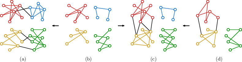
Refer to caption — Figure 1: A sequence of graphs with four prominent clusters each colored differently. Black edges connect different clusters and forward (resp. backward) arrows indicate additions (resp. deletions) of vertices and edges. From (a) to (b), two clusters split; from (b) to (c), two clusters merge; from (c) to (d), one cluster disappears.

Algorithms for both zigzag and non-zigzag persistence have a general-case time complexity of $O(m^{\omega})$ [4, 12, 19, 20], where $m$ is the length of the input filtration and $\omega<2.37286$ is the matrix multiplication exponent [2]. For the special case of graph filtrations, it is well known that non-zigzag persistence can be computed in $O(m\,\alpha(m))$ time, where $\alpha(m)$ is the inverse Ackermann’s function that is almost constant for all practical purposes [5]. However, analogous faster algorithms for zigzag persistence on graphs are not known. In this paper, we present algorithms for zigzag persistence on graphs with near-linear time complexity. In particular, given a zigzag filtration of length $m$ for a graph with $n$ vertices and edges, our algorithm for 0-dimension runs in $O(m\log^{2}n+m\log m)$ time, and our algorithm for $1$ -dimension runs in $O(m\log^{4}n)$ time. Observe that the algorithm for $0$ -dimension works for arbitrary complexes by restricting to the $1$ -skeletons.

The difficulty in designing faster zigzag persistence algorithms for the special case of graphs lies in the deletion of vertices and edges. For example, besides merging into bigger ones, connected components can also split into smaller ones because of edge deletion. Therefore, one cannot simply kill the younger component during merging as in standard persistence [12], but rather has to pair the merge and departure events with the split and entrance events (see Sections 3 for details). Similarly, in dimension one, deletion of edges may kill 1-cycles so that one has to properly pair the creation and destruction of 1-cycles, instead of simply treating all 1-dimensional intervals as infinite ones.

Our solutions are as follows: in dimension zero, we find that the $O(n\log n)$ algorithm by Agarwal et al. [1] originally designed for pairing critical points of Morse functions on 2-manifolds can be utilized in our scenario. We formally prove the correctness of applying the algorithm and use a dynamic connectivity data structure [16] to achieve the claimed complexity. In dimension one, we observe that a positive and a negative edge can be paired by finding the earliest 1-cycle containing both edges which resides in all intermediate graphs. We further reduce the pairing to finding the max edge-weight of a path in a minimum spanning forest. Utilizing a data structure for dynamic minimum spanning forest [16], we achieve the claimed time complexity. Section 4 details this algorithm.

Using Alexander duality, we also extend the algorithm for $0$ -dimension to compute $(p-1)$ -dimensional zigzag for $\mathbb{R}^{p}$ -embedded complexes. The connection between these two cases for non-zigzag persistence is well known [11, 23], and the challenge comes in adopting this duality to the zigzag setting while maintaining an efficient time budget. With the help of a dual filtration and an observation about faster void boundary reconstruction for $(p-1)$ -connected complexes [10], we achieve a time complexity of $O(m\log^{2}n+m\log m+n\log n)$ .

Related works.

The algorithm for computing persistent homology by Edelsbrunner et al. [12] is a cornerstone of topological data analysis. Several extensions followed after this initial development. De Silva et al. [7] proposed to compute persistent cohomology instead of homology which gives the same barcode. De Silva et al. [6] then showed that the persistent cohomology algorithm runs faster in practice than the version that uses homology. The annotation technique proposed by Dey et al. [9] implements the cohomology algorithm by maintaining a cohomology basis more succinctly and extends to towers connected by simplicial maps. These algorithms run in $O(m^{3})$ time.

Carlsson and de Silva [3] introduced zigzag persistence as an extension of the standard persistence, where they also presented a decomposition algorithm for computing zigzag barcodes on the level of vector spaces and linear maps. This algorithm is then adapted to zigzag filtrations at simplicial level by Carlsson et al. [4] with a time complexity of $O(m^{3})$ . Both algorithms [3, 4] utilize a construct called right filtration and a birth-time vector. Maria and Oudot [19] proposed an algorithm for zigzag persistence based on some diamond principles where an inverse non-zigzag filtration is always maintained during the process. The algorithm in [19] is shown to run faster in experiments than the algorithm in [4] though the time complexities remain the same. Milosavljević et al. [20] proposed an algorithm for zigzag persistence based on matrix multiplication which runs in $O(m^{\omega})$ time, giving the best asymptotic bound for computing zigzag and non-zigzag persistence in general dimensions.

The algorithms reviewed so far are all for general dimensions and many of them are based on matrix operations. Thus, it is not surprising that the best time bound achieved is $O(m^{\omega})$ given that computing Betti numbers for a simplicial $2$ -complex of size $m$ is as hard as computing the rank of a $\mathbb{Z}_{2}$ -matrix with $m$ non-zero entries as shown by Edelsbrunner and Parsa [13]. To lower the complexity, one strategy (which is adopted by this paper) is to consider special cases where matrix operations can be avoided. The work by Dey [8] is probably most related to ours in that regard, who proposed an $O(m\log m)$ algorithm for non-zigzag persistence induced from height functions on $\mathbb{R}^{3}$ -embedded complexes.

2 Preliminaries

A zigzag module (or module for short) is a sequence of vector spaces

\mathcal{M}:V_{0}\xleftrightarrow{\;\psi_{0}\;}V_{1}\xleftrightarrow{\;\psi_{1}\;}\cdots\xleftrightarrow{\;\psi_{m-1}\;}V_{m}

in which each $\psi_{i}$ is either a forward linear map $\psi_{i}:V_{i}\to V_{i+1}$ or a backward linear map $\psi_{i}:V_{i}\leftarrow V_{i+1}$ . We assume vector spaces are over field $\mathbb{Z}_{2}$ in this paper. A module $\mathcal{S}$ of the form

\mathcal{S}:W_{0}\xleftrightarrow{\;\phi_{0}\;}W_{1}\xleftrightarrow{\;\phi_{1}\;}\cdots\xleftrightarrow{\;\phi_{m-1}\;}W_{m}

is called a submodule of $\mathcal{M}$ if each $W_{i}$ is a subspace of $V_{i}$ and each $\phi_{i}$ is the restriction of $\psi_{i}$ . For an interval $[b,d]\subseteq[0,m]$ , $\mathcal{S}$ is called an interval submodule of $\mathcal{M}$ over $[b,d]$ if $W_{i}$ is one-dimensional for $i\in[b,d]$ and is trivial for $i\not\in[b,d]$ , and $\phi_{i}$ is an isomorphism for $i\in[b,d-1]$ . It is well known [3] that $\mathcal{M}$ admits an interval decomposition $\mathcal{M}=\bigoplus_{\alpha\in\mathcal{A}}\mathcal{I}^{[b_{\alpha},d_{\alpha}]}$ which is a direct sum of interval submodules of $\mathcal{M}$ . The (multi-)set of intervals $\{[b_{\alpha},d_{\alpha}]\,|\,\alpha\in\mathcal{A}\}$ is called the zigzag barcode (or barcode for short) of $\mathcal{M}$ and is denoted as $\mathsf{Pers}(\mathcal{M})$ . Each interval in a zigzag barcode is called a persistence interval.

In this paper, we mainly focus on a special type of zigzag modules:

Definition 1 (Elementary zigzag module).

A zigzag module is called elementary if it starts with the trivial vector space and all linear maps in the module are of the three forms: (i) an isomorphism; (ii) an injection with rank 1 cokernel; (iii) a surjection with rank 1 kernel.

A zigzag filtration (or filtration for short) is a sequence of simplicial complexes

\mathcal{F}:K_{0}\xleftrightarrow{\;\sigma_{0}\;}K_{1}\xleftrightarrow{\;\sigma_{1}\;}\cdots\xleftrightarrow{\;\sigma_{m-1}\;}K_{m}

in which each $K_{i}\xleftrightarrow{\;\sigma_{i}\;}K_{i+1}$ is either a forward inclusion $K_{i}\hookrightarrow K_{i+1}$ with a single simplex $\sigma_{i}$ added, or a backward inclusion $K_{i}\hookleftarrow K_{i+1}$ with a single $\sigma_{i}$ deleted. When the $\sigma_{i}$ ’s are not explicitly used, we drop them and simply denote $\mathcal{F}$ as $\mathcal{F}:K_{0}\leftrightarrow K_{1}\leftrightarrow\cdots\leftrightarrow K_{m}$ . For computational purposes, we sometimes assume that a filtration starts with the empty complex, i.e., $K_{0}=\varnothing$ in $\mathcal{F}$ . Throughout the paper, we also assume that each $K_{i}$ in $\mathcal{F}$ is a subcomplex of a fixed complex $K$ ; such a $K$ , when not given, can be constructed by taking the union of every $K_{i}$ in $\mathcal{F}$ . In this case, we call $\mathcal{F}$ a filtration of $K$ .

Applying the $p$ -th homology with $\mathbb{Z}_{2}$ coefficients on $\mathcal{F}$ , we derive the $p$ -th zigzag module of $\mathcal{F}$

\mathsf{H}_{p}(\mathcal{F}):\mathsf{H}_{p}(K_{0})\xleftrightarrow{\;\varphi^{p}_{0}\;}\mathsf{H}_{p}(K_{1})\xleftrightarrow{\;\varphi^{p}_{1}\;}\cdots\xleftrightarrow{\;\varphi^{p}_{m-1}\;}\mathsf{H}_{p}(K_{m})

in which each $\varphi^{p}_{i}$ is the linear map induced by the inclusion. In this paper, whenever $\mathcal{F}$ is used to denote a filtration, we use $\varphi^{p}_{i}$ to denote a linear map in the module $\mathsf{H}_{p}(\mathcal{F})$ . Note that $\mathsf{H}_{p}(\mathcal{F})$ is an elementary module if $\mathcal{F}$ starts with an empty complex. Specifically, we call $\mathsf{Pers}(\mathsf{H}_{p}(\mathcal{F}))$ the $p$ -th zigzag barcode of $\mathcal{F}$ .

3 Zero-dimensional zigzag persistence

We present our algorithm for 0-th zigzag persistence¹¹ 1 For brevity, henceforth we call $p$ -dimensional zigzag persistence as $p$ -th zigzag persistence. in this section. The input is assumed to be on graphs but note that our algorithm can be applied to any complex by restricting to its 1-skeleton. We first define the barcode graph of a zigzag filtration which is a construct that our algorithm implicitly works on. In a barcode graph, nodes correspond to connected components of graphs in the filtration and edges encode the mapping between the components:

Definition 2 (Barcode graph).

For a graph $G$ and a zigzag filtration $\mathcal{F}:G_{0}\leftrightarrow G_{1}\leftrightarrow\cdots\leftrightarrow G_{m}$ of $G$ , the barcode graph $\mathbb{G}_{\mathrm{B}}(\mathcal{F})$ of $\mathcal{F}$ is a graph whose vertices (preferably called nodes) are associated with a level and whose edges connect nodes only at adjacent levels. The graph $\mathbb{G}_{\mathrm{B}}(\mathcal{F})$ is constructively described as follows:

•

For each $G_{i}$ in $\mathcal{F}$ and each connected component of $G_{i}$ , there is a node in $\mathbb{G}_{\mathrm{B}}(\mathcal{F})$ at level $i$ corresponding to this component; this node is also called a level- $i$ node.
•

For each inclusion $G_{i}\leftrightarrow G_{i+1}$ in $\mathcal{F}$ , if it is forward, then there is an edge connecting a level- $i$ node $v_{i}$ to a level- $(i+1)$ node $v_{i+1}$ if and only if the component of $v_{i}$ maps to the component of $v_{i+1}$ by the inclusion. Similarly, if the inclusion is backward, then $v_{i}$ connects to $v_{i+1}$ by an edge iff the component of $v_{i+1}$ maps to the component of $v_{i}$ .

For two nodes at different levels in $\mathbb{G}_{\mathrm{B}}(\mathcal{F})$ , the node at the higher (resp. lower) level is said to be higher (resp. lower) than the other.

Remark 3.

Note that some works [8, 18] also have used similar notions of barcode graphs.

Figure 2(a) and 2(b) give an example of a zigzag filtration and its barcode graph. Note that a barcode graph is of size $O(mn)$ , where $m$ is the length of $\mathcal{F}$ and $n$ is the number of vertices and edges of $G$ . Although we present our algorithm (Algorithm 1) by first building the barcode graph, the implementation does not do so explicitly, allowing us to achieve the claimed time complexity; see Section 3.1 for the implementation details. Introducing barcode graphs helps us justify the algorithm, and more importantly, points to the fact that the algorithm can be applied whenever such a barcode graph can be built.

Algorithm 1 (Algorithm for 0-th zigzag persistence).

Given a graph $G$ and a zigzag filtration $\mathcal{F}:\varnothing=G_{0}\leftrightarrow G_{1}\leftrightarrow\cdots\leftrightarrow G_{m}$ of $G$ , we first build the barcode graph $\mathbb{G}_{\mathrm{B}}(\mathcal{F})$ , and then apply the pairing algorithm described in [1] on $\mathbb{G}_{\mathrm{B}}(\mathcal{F})$ to compute $\mathsf{Pers}(\mathsf{H}_{0}(\mathcal{F}))$ . For a better understanding, we rephrase this algorithm which originally works on Reeb graphs:

The algorithm iterates for $i=0,\ldots,m-1$ and maintains a barcode forest $T_{i}$ , whose leaves have a one-to-one correspondence to level- $i$ nodes of $\mathbb{G}_{\mathrm{B}}(\mathcal{F})$ . Like the barcode graph, each tree node in a barcode forest is associated with a level and each tree edge connects nodes at adjacent levels. For each tree in a barcode forest, the lowest node is the root. Initially, $T_{0}$ is empty; then, the algorithm builds $T_{i+1}$ from $T_{i}$ in the $i$ -th iteration. Intervals for $\mathsf{Pers}(\mathsf{H}_{0}(\mathcal{F}))$ are produced while updating the barcode forest. (Figure 2(c) illustrates such updates.)

Specifically, the $i$ -th iteration proceeds as follows: first, $T_{i+1}$ is formed by copying the level- $(i+1)$ nodes of $\mathbb{G}_{\mathrm{B}}(\mathcal{F})$ and their connections to the level- $i$ nodes, into $T_{i}$ ; the copying is possible because leaves of $T_{i}$ and level- $i$ nodes of $\mathbb{G}_{\mathrm{B}}(\mathcal{F})$ have a one-to-one correspondence; see transitions from $T_{5}$ to $T_{6}$ and from $T_{9}$ to $T_{10}$ in Figure 2(c). We further change $T_{i+1}$ under the following events:

Entrance:: One level- $(i+1)$ node in $T_{i+1}$ , said to be entering, does not connect to any level- $i$ node.
Split:: One level- $i$ node in $T_{i+1}$ , said to be splitting, connects to two different level- $(i+1)$ nodes. For the two events so far, no changes need to be made on $T_{i+1}$ .
Departure:: One level- $i$ node $u$ in $T_{i+1}$ , said to be departing, does not connect to any level- $(i+1)$ node. If $u$ has splitting ancestors (i.e., ancestors which are also splitting nodes), add an interval $[j+1,i]$ to $\mathsf{Pers}(\mathsf{H}_{0}(\mathcal{F}))$ , where $j$ is the level of the highest splitting ancestor $v$ of $u$ ; otherwise, add an interval $[j,i]$ to $\mathsf{Pers}(\mathsf{H}_{0}(\mathcal{F}))$ , where $j$ is the level of the root $v$ of $u$ . We then delete the path from $v$ to $u$ in $T_{i+1}$ .
Merge:: Two different level- $i$ nodes $u_{1},u_{2}$ in $T_{i+1}$ connect to the same level- $(i+1)$ node. Tentatively, $T_{i+1}$ may now contain a loop and is not a tree. If $u_{1},u_{2}$ are in different trees in $T_{i}$ , add an interval $[j,i]$ to $\mathsf{Pers}(\mathsf{H}_{0}(\mathcal{F}))$ , where $j$ is the level of the higher root of $u_{1},u_{2}$ in $T_{i}$ ; otherwise, add an interval $[j+1,i]$ to $\mathsf{Pers}(\mathsf{H}_{0}(\mathcal{F}))$ , where $j$ is the level of the highest common ancestor of $u_{1},u_{2}$ in $T_{i}$ . We then glue the two paths from $u_{1}$ and $u_{2}$ to their level- $j$ ancestors in $T_{i+1}$ , after which $T_{i+1}$ is guaranteed to be a tree.
No-change:: If none of the above events happen, no changes are made on $T_{i+1}$ .

At the end, for each root in $T_{m}$ at a level $j$ , add an interval $[j,m]$ to $\mathsf{Pers}(\mathsf{H}_{0}(\mathcal{F}))$ , and for each splitting node in $T_{m}$ at a level $j$ , add an interval $[j+1,m]$ to $\mathsf{Pers}(\mathsf{H}_{0}(\mathcal{F}))$ .

Remark 4.

The justification of Algorithm 1 is given in Section 3.2.

Figure 2(c) gives examples of barcode forests constructed by Algorithm 1 for the barcode graph shown in Figure 2(b), where $T_{1}$ and $T_{2}$ introduce entering nodes, $T_{6}$ introduces a splitting node, and $T_{10}$ introduces a departing node. In $T_{10}$ , the departure event happens and the dotted path is deleted, producing an interval $[8,9]$ . In $T_{3}$ and $T_{9}$ , the merge event happens and the dotted paths are glued together, producing intervals $[2,2]$ and $[6,8]$ . Note that the glued level- $i$ nodes are in different trees in $T_{3}$ and are in the same tree in $T_{9}$ .

3.1 Implementation

As mentioned, to achieve the claimed time complexity, we do not explicitly build the barcode graph. Instead, we differentiate the different events as follows: inserting (resp. deleting) a vertex in $\mathcal{F}$ simply corresponds to the entrance (resp. departure) event, whereas inserting (resp. deleting) an edge corresponds to the merge (resp. split) event only when connected components in the graph merge (resp. split).

To keep track of the connectivity of vertices, we use a dynamic connectivity data structure by Holm et al. [16], which we denote as $\mathbb{D}$ . Assuming that $m$ is the length of $\mathcal{F}$ and $n$ is the number of vertices and edges of $G$ , the data structure $\mathbb{D}$ supports the following operations:

•

Return the identifier²² 2 Since $\mathbb{D}$ maintains the connectivity information by dynamically updating the spanning forest for the current graph, the identifier of a connected component is indeed the identifier of a tree in the spanning forest. of the connected component of a vertex $v$ in $O(\log n)$ time. We denote this subroutine as $\mathtt{find}(v)$ .
•

Insert or delete an edge, and possibly update the connectivity information, in $O(\log^{2}n)$ amortized time.

We also note the following implementation details:

•

All vertices of $G$ are added to $\mathbb{D}$ initially and are then never deleted. But we make sure that edges in $\mathbb{D}$ always equal edges in $G_{i}$ as the algorithm proceeds so that $\mathbb{D}$ still records the connectivity of $G_{i}$ .
•

At each iteration $i$ , we update $T_{i}$ to form $T_{i+1}$ according to the changes of the connected components from $G_{i}$ to $G_{i+1}$ . For this, we maintain a key-value map $\phi$ from connected components of $\mathbb{D}$ to leaves of the barcode forest, and $\phi$ is initially empty.
•

In a barcode forest $T_{i}$ , since the level of a leaf always equals $i$ , we only record the level of a non-leaf node. Note that at iteration $i$ , a leaf in $T_{i}$ may uniquely connect to a single leaf in $T_{i+1}$ . In this case, we simply let the leaf in $T_{i}$ automatically become a leaf in $T_{i+1}$ ; see Figure 3. The size of a barcode forest is then $O(m)$ .

Now we can present the full detail of the implementation. Specifically, for each addition and deletion in $\mathcal{F}$ , we do the following in each case:

Adding vertex $\sigma_{i}=v$ :: Add an isolated node to the barcode forest and let $\phi(\mathtt{find}(v))$ equal this newly added node.
Deleting vertex $\sigma_{i}=v$ :: Let $\ell=\phi(\mathtt{find}(v))$ ; then, $\ell$ is the node in the barcode forest that is departing. Update the barcode forest as described in Algorithm 1.
Adding edge $\sigma_{i}=(u,v)$ :: Let $t_{1}=\mathtt{find}(u)$ , $t_{2}=\mathtt{find}(v)$ , $\ell_{1}=\phi(t_{1})$ , and $\ell_{2}=\phi(t_{2})$ . If $t_{1}=t_{2}$ , then the no-change event happens; otherwise, the merge event happens. We then add $(u,v)$ to $\mathbb{D}$ . For the no-change event, do nothing after this. For the merge event, do the following: glue the paths from $\ell_{1}$ and $\ell_{2}$ to their ancestors as described in Algorithm 1; attach a new child $\ell$ to the highest glued node; update $\phi(\mathtt{find}(u))$ to be $\ell$ .
Deleting edge $\sigma_{i}=(u,v)$ :: Let $\ell=\phi(\mathtt{find}(u))$ , and then delete $(u,v)$ from $\mathbb{D}$ . If $\mathtt{find}(u)=\mathtt{find}(v)$ after this, then the no-change event happens but we have to update $\phi(\mathtt{find}(u))$ to be $\ell$ because the identifiers of the connected components in $\mathbb{D}$ may change after deleting the edge [16]. Otherwise, the split event happens: we attach two new children $\ell_{1}$ , $\ell_{2}$ to $\ell$ in the barcode forest and set $\phi(\mathtt{find}(u))=\ell_{1}$ , $\phi(\mathtt{find}(v))=\ell_{2}$ .

Mergeable trees.

Following the idea in [1], the barcode forest can be implemented using the mergeable trees data structure by Georgiadis et al. [14]. Since the maximum number of nodes in a barcode forest is $O(m)$ , the data structure supports the following operations, each of which takes $O(\log m)$ amortized time:

•

Return the root of a node.
•

Return the nearest common ancestor of two leaves (in the same tree).
•

Glue the paths from two leaves (in the same tree) to their nearest common ancestor.

Note that while we delete the path from the departing node to its ancestor in the departure event, deletions are not supported by mergeable trees. However, path deletions are indeed unnecessary which are only meant for a clear exposition. Hence, during implementation, we only traverse each ancestor of the departing node until an unpaired³³ 3 An entering or splitting node is initially unpaired when introduced and becomes paired when its level is used to produce an interval. E.g., the node $v$ becomes paired in the departure event in Algorithm 1. one is found without actual deletions. Since each node can only be traversed once, the traversal in the departure events takes $O(m)$ time in total. See [14, Section 5] for details of implementing the barcode forest and its operations using mergeable trees.

Complexity.

The time complexity of the algorithm is $O(m\log^{2}n+m\log m)$ dominated by the operations of the dynamic connectivity and the mergeable trees data structures.

3.2 Justification

In this subsection, we justify the correctness of Algorithm 1. For each entering node $u$ in a $T_{i}$ of Algorithm 1, there must be a single node in $\mathbb{G}_{\mathrm{B}}(\mathcal{F})$ at the level of $u$ with the same property. So we also have entering nodes in $\mathbb{G}_{\mathrm{B}}(\mathcal{F})$ . Splitting and departing nodes in $\mathbb{G}_{\mathrm{B}}(\mathcal{F})$ can be similarly defined.

We first prepare some standard notions and facts in zigzag persistence (Definition 5 and 7, Proposition 9) that help with our proofs. Some notions also appear in previous works in different forms; see, e.g., [19].

Definition 5 (Representatives).

Let $\mathcal{M}:V_{0}\xleftrightarrow{\;\psi_{0}\;}\cdots\xleftrightarrow{\;\psi_{m-1}\;}V_{m}$ be an elementary zigzag module and $[s,t]\subseteq[1,m]$ be an interval. An indexed set $\{\alpha_{i}\in V_{i}\,|\,i\in[s,t]\}$ is called a set of partial representatives for $[s,t]$ if for every $i\in[s,t-1]$ , $\alpha_{i}\mapsto\alpha_{i+1}$ or $\alpha_{i}\mapsfrom\alpha_{i+1}$ by $\psi_{i}$ ; it is called a set of representatives for $[s,t]$ if the following additional conditions are satisfied:

1.

If $\psi_{s-1}:V_{s-1}\rightarrow V_{s}$ is forward with non-trivial cokernel, then $\alpha_{s}$ is not in $\mathsf{img}(\psi_{s-1})$ ; if $\psi_{s-1}:V_{s-1}\leftarrow V_{s}$ is backward with non-trivial kernel, then $\alpha_{s}$ is the non-zero element in $\mathsf{ker}(\psi_{s-1})$ .
2.

If $t<m$ and $\psi_{t}:V_{t}\leftarrow V_{t+1}$ is backward with non-trivial cokernel, then $\alpha_{t}$ is not in $\mathsf{img}(\psi_{t})$ ; if $t<m$ and $\psi_{t}:V_{t}\rightarrow V_{t+1}$ is forward with non-trivial kernel, then $\alpha_{t}$ is the non-zero element in $\mathsf{ker}(\psi_{t})$ .

Specifically, when $\mathcal{M}:=\mathsf{H}_{p}(\mathcal{F})$ for a zigzag filtration $\mathcal{F}$ , we use terms $p$ -representatives and partial $p$ -representatives to emphasize the dimension $p$ .

Remark 6.

Let $\mathcal{F}$ be the filtration given in Figure 2(a), and let $\alpha_{8}$ , $\alpha_{9}$ be the sum of the component containing vertex 1 and the component containing vertex 2 in $G_{8}$ and $G_{9}$ . Then, $\{\alpha_{8},\alpha_{9}\}$ is a set of 0-representatives for the interval $[8,9]\in\mathsf{Pers}(\mathsf{H}_{0}(\mathcal{F}))$ .

Definition 7 (Positive/negative indices).

Let $\mathcal{M}:V_{0}\xleftrightarrow{\;\psi_{0}\;}\cdots\xleftrightarrow{\;\psi_{m-1}\;}V_{m}$ be an elementary zigzag module. The set of positive indices of $\mathcal{M}$ , denoted $\mathsf{P}(\mathcal{M})$ , and the set of negative indices of $\mathcal{M}$ , denoted $\mathsf{N}(\mathcal{M})$ , are constructed as follows: for each forward $\psi_{i}:V_{i}\to V_{i+1}$ , if $\psi_{i}$ is an injection with non-trivial cokernel, add $i+1$ to $\mathsf{P}(\mathcal{M})$ ; if $\psi_{i}$ is a surjection with non-trivial kernel, add $i$ to $\mathsf{N}(\mathcal{M})$ . Furthermore, for each backward $\psi_{i}:V_{i}\leftarrow V_{i+1}$ , if $\psi_{i}$ is an injection with non-trivial cokernel, add $i$ to $\mathsf{N}(\mathcal{M})$ ; if $\psi_{i}$ is a surjection with non-trivial kernel, add $i+1$ to $\mathsf{P}(\mathcal{M})$ . Finally, add $\mathsf{rank}\,V_{m}$ copies of $m$ to $\mathsf{N}(\mathcal{M})$ .

Remark 8.

For each $\psi_{i}:V_{i}\leftrightarrow V_{i+1}$ in Definition 7, if $i+1\in\mathsf{P}(\mathcal{M})$ , then $i\not\in\mathsf{N}(\mathcal{M})$ ; similarly, if $i\in\mathsf{N}(\mathcal{M})$ , then $i+1\not\in\mathsf{P}(\mathcal{M})$ . Furthermore, if $\psi_{i}$ is an isomorphism, then $i\not\in\mathsf{N}(\mathcal{M})$ and $i+1\not\in\mathsf{P}(\mathcal{M})$ .

Note that $\mathsf{N}(\mathcal{M})$ in Definition 7 is in fact a multi-set; calling it a set should not cause any confusion in this paper though. Also note that $|\mathsf{P}(\mathcal{M})|=|\mathsf{N}(\mathcal{M})|$ , and every index in $\mathsf{P}(\mathcal{M})$ (resp. $\mathsf{N}(\mathcal{M})$ ) is the start (resp. end) of an interval in $\mathsf{Pers}(\mathcal{M})$ . This explains why we add $\mathsf{rank}\,V_{m}$ copies of $m$ to $\mathsf{N}(\mathcal{M})$ because there are always $\mathsf{rank}\,V_{m}$ number of intervals ending with $m$ in $\mathsf{Pers}(\mathcal{M})$ ; see the example in Figure 2(a) where $\mathsf{rank}\,\mathsf{H}_{0}(G_{10})=2$ .

Proposition 9.

Let $\mathcal{M}$ be an elementary zigzag module and $\pi:\mathsf{P}(\mathcal{M})\to\mathsf{N}(\mathcal{M})$ be a bijection. If every $b\in\mathsf{P}(\mathcal{M})$ satisfies that $b\leq\pi(b)$ and the interval $[b,\pi(b)]$ has a set of representatives, then $\mathsf{Pers}(\mathcal{M})=\{[b,\pi(b)]\,|\,b\in\mathsf{P}(\mathcal{M})\}$ .

Proof.

For each $b\in\mathsf{P}(\mathcal{M})$ , let $\big\{\alpha^{b}_{j}\,|\,j\in[b,\pi(b)]\big\}$ be a set of representatives for $[b,\pi(b)]$ . Then, define $\mathcal{I}^{[b,\pi(b)]}$ as an interval submodule of $\mathcal{M}$ over $[b,\pi(b)]$ such that $\mathcal{I}^{[b,\pi(b)]}(j)$ is generated by $\alpha^{b}_{j}$ if $j\in[b,\pi(b)]$ and is trivial otherwise, where $\mathcal{I}^{[b,\pi(b)]}(j)$ denotes the $j$ -th vector space in $\mathcal{I}^{[b,\pi(b)]}$ . We claim that $\mathcal{M}=\bigoplus_{b\in\mathsf{P}(\mathcal{M})}\mathcal{I}^{[b,\pi(b)]}$ , which implies the proposition. To prove this, suppose that $\mathcal{M}$ is of the form

\mathcal{M}:V_{0}\xleftrightarrow{\;\psi_{0}\;}V_{1}\xleftrightarrow{\;\psi_{1}\;}\cdots\xleftrightarrow{\;\psi_{m-1}\;}V_{m}

Then, we only need to verify that for every $i\in[0,m]$ , the set $\big\{\alpha^{b}_{i}\,|\,b\in\mathsf{P}(\mathcal{M})\text{ and }[b,\pi(b)]\ni i\big\}$ is a basis of $V_{i}$ . We prove this by induction on $i$ . For $i=0$ , since $V_{0}=0$ , $\big\{\alpha^{b}_{0}\,|\,b\in\mathsf{P}(\mathcal{M})\text{ and }[b,\pi(b)]\ni 0\big\}=\varnothing$ is obviously a basis. So we can assume that for an $i\in[0,m-1]$ , $\big\{\alpha^{b}_{i}\,|\,b\in\mathsf{P}(\mathcal{M})\text{ and }[b,\pi(b)]\ni i\big\}$ is a basis of $V_{i}$ . We have the following cases:

$\psi_{i}$ an isomorphism:: In this case, $i\not\in\mathsf{N}(\mathcal{M})$ and $i+1\not\in\mathsf{P}(\mathcal{M})$ . If $\psi_{i}:V_{i}\to V_{i+1}$ is forward, then $\big\{\alpha^{b}_{i+1}\,|\,b\in\mathsf{P}(\mathcal{M})\text{ and }[b,\pi(b)]\ni i+1\big\}=\big\{\psi_{i}(\alpha^{b}_{i})\,|\,b\in\mathsf{P}(\mathcal{M})\text{ and }[b,\pi(b)]\ni i\big\}$ . The elements in $\big\{\alpha^{b}_{i+1}\,|\,b\in\mathsf{P}(\mathcal{M})\text{ and }[b,\pi(b)]\ni i+1\big\}$ must then form a basis of $V_{i+1}$ because $\psi_{i}$ is an isomorphism. The verification for $\psi_{i}$ being backward is similar.
$\psi_{i}:V_{i}\to V_{i+1}$ forward, $\mathsf{coker}(\psi_{i})$ non-trivial:: In this case, $i\not\in\mathsf{N}(\mathcal{M})$ and $i+1\in\mathsf{P}(\mathcal{M})$ . For each $b\in\mathsf{P}(\mathcal{M})$ such that $[b,\pi(b)]\ni i$ , $[b,\pi(b)]\ni i+1$ and $\alpha^{b}_{i}\mapsto\alpha^{b}_{i+1}$ by $\psi_{i}$ . We then have that elements in $\big\{\alpha^{b}_{i+1}=\psi_{i}(\alpha^{b}_{i})\,|\,b\in\mathsf{P}(\mathcal{M})\text{ and }[b,\pi(b)]\ni i\big\}$ are linearly independent because $\psi_{i}$ is injective. Since $\alpha^{i+1}_{i+1}\not\in\mathsf{img}(\psi_{i})$ by Definition 5, $\big\{\alpha^{b}_{i+1}\,|\,b\in\mathsf{P}(\mathcal{M})\text{ and }[b,\pi(b)]\ni i+1\big\}=\big\{\alpha^{b}_{i+1}\,|\,b\in\mathsf{P}(\mathcal{M})\text{ and }[b,\pi(b)]\ni i\big\}\cup\big\{\alpha^{i+1}_{i+1}\big\}$ must contain linearly independent elements. The fact that the cardinality of the set equals $\mathsf{rank}\,V_{i+1}$ implies that it must form a basis of $V_{i+1}$ .
$\psi_{i}:V_{i}\to V_{i+1}$ forward, $\mathsf{ker}(\psi_{i})$ non-trivial:: In this case, $i\in\mathsf{N}(\mathcal{M})$ and $i+1\not\in\mathsf{P}(\mathcal{M})$ . Let $j=\pi^{-1}(i)$ . For each $b\in\mathsf{P}(\mathcal{M})$ such that $[b,\pi(b)]\ni i$ and $b\neq j$ , $[b,\pi(b)]\ni i+1$ and $\alpha^{b}_{i}\mapsto\alpha^{b}_{i+1}$ by $\psi_{i}$ . We then have that $\big\{\alpha^{b}_{i+1}\,|\,b\in\mathsf{P}(\mathcal{M})\text{ and }[b,\pi(b)]\ni i+1\big\}=\big\{\psi_{i}\big(\alpha^{b}_{i}\big)\,|\,b\in\mathsf{P}(\mathcal{M})\text{ and }[b,\pi(b)]\ni i\big\}\setminus\big\{\psi_{i}\big(\alpha_{i}^{j}\big)\big\}$ . Since $\psi_{i}$ is surjective, elements in $\big\{\psi_{i}\big(\alpha_{i}^{b}\big)\,|\,b\in\mathsf{P}(\mathcal{M})\text{ and }[b,\pi(b)]\ni i\big\}$ generate $V_{i+1}$ , in which $\psi_{i}\big(\alpha_{i}^{j}\big)=0$ by Definition 5. It follows that $\big\{\alpha^{b}_{i+1}\,|\,b\in\mathsf{P}(\mathcal{M})\text{ and }[b,\pi(b)]\ni i+1\big\}$ forms a basis of $V_{i+1}$ because it generates $V_{i+1}$ and its cardinality equals $\mathsf{rank}\,V_{i+1}$ .
$\psi_{i}:V_{i}\leftarrow V_{i+1}$ backward, $\mathsf{coker}(\psi_{i})$ non-trivial:: In this case, $i\in\mathsf{N}(\mathcal{M})$ and $i+1\not\in\mathsf{P}(\mathcal{M})$ . For each $b\in\mathsf{P}(\mathcal{M})$ such that $[b,\pi(b)]\ni i$ and $\pi(b)\neq i$ , $[b,\pi(b)]\ni i+1$ and $\alpha^{b}_{i}\mapsfrom\alpha^{b}_{i+1}$ by $\psi_{i}$ . We then have that elements in $\big\{\alpha^{b}_{i+1}=(\psi_{i})^{-1}(\alpha^{b}_{i})\,|\,b\in\mathsf{P}(\mathcal{M}),\,[b,\pi(b)]\ni i,\,\text{and}\,\pi(b)\neq i\big\}$ are linearly independent because if they are not, then their images under $\psi_{i}$ are also not, which is a contradiction. Note that $\big\{\alpha^{b}_{i+1}\,|\,b\in\mathsf{P}(\mathcal{M}),[b,\pi(b)]\ni i+1\big\}=\big\{\alpha^{b}_{i+1}\,|\,b\in\mathsf{P}(\mathcal{M}),\,[b,\pi(b)]\ni i,\,\text{and}\,\pi(b)\neq i\big\}$ and its cardinality equals $\mathsf{rank}\,V_{i+1}$ , so it must form a basis of $V_{i+1}$ .
$\psi_{i}:V_{i}\leftarrow V_{i+1}$ backward, $\mathsf{ker}(\psi_{i})$ non-trivial:: In this case, $i\not\in\mathsf{N}(\mathcal{M})$ and $i+1\in\mathsf{P}(\mathcal{M})$ . For each $b\in\mathsf{P}(\mathcal{M})$ such that $[b,\pi(b)]\ni i$ , $[b,\pi(b)]\ni i+1$ and $\alpha^{b}_{i}\mapsfrom\alpha^{b}_{i+1}$ by $\psi_{i}$ . We then have that elements in $\big\{\alpha^{b}_{i+1}\in(\psi_{i})^{-1}(\alpha^{b}_{i})\,|\,b\in\mathsf{P}(\mathcal{M})\text{ and }[b,\pi(b)]\ni i\big\}$ are linearly independent because their images under $\psi_{i}$ are. We also have that there is no non-trivial linear combination of $\big\{\alpha^{b}_{i+1}\,|\,b\in\mathsf{P}(\mathcal{M})\text{ and }[b,\pi(b)]\ni i\big\}$ falling in $\mathsf{ker}(\psi_{i})$ because otherwise their images under $\psi_{i}$ would not be linearly independent. Since $\alpha_{i+1}^{i+1}$ is the non-zero element in $\mathsf{ker}(\psi_{i})$ by Definition 5, we have that $\big\{\alpha^{b}_{i+1}\,|\,b\in\mathsf{P}(\mathcal{M})\text{ and }[b,\pi(b)]\ni i+1\big\}=\big\{\alpha^{b}_{i+1}\,|\,b\in\mathsf{P}(\mathcal{M})\text{ and }[b,\pi(b)]\ni i\big\}\cup\big\{\alpha_{i+1}^{i+1}\big\}$ contains linearly independent elements. Then, it must form a basis of $V_{i+1}$ because its cardinality equals $\mathsf{rank}\,V_{i+1}$ , ∎

Now we present several propositions leading to our conclusion (Theorem 14). Specifically, Proposition 10 states that a certain path in $\mathbb{G}_{\mathrm{B}}(\mathcal{F})$ induces a set of partial 0-representatives. Proposition 11 lists some invariants of Algorithm 1. Proposition 10 and 11 support the proof of Proposition 13, which together with Proposition 9 implies Theorem 14.

From now on, $G$ and $\mathcal{F}$ always denote the input to Algorithm 1. Since each node in a barcode graph represents a connected component, we also interpret nodes in a barcode graph as 0-th homology classes throughout the paper. Moreover, a path in a barcode graph from a node $v$ to a node $u$ is said to be within level $j$ and $i$ if for each node on the path, its level $\ell$ satisfies $j\leq\ell\leq i$ ; we denote such a path as $(v\rightsquigarrow u)_{[j,i]}$ .

Proposition 10.

Let $v$ be a level- $j$ node and $u$ be a level- $i$ node in $\mathbb{G}_{\mathrm{B}}(\mathcal{F})$ such that $j<i$ and there is a path $(v\rightsquigarrow u)_{[j,i]}$ in $\mathbb{G}_{\mathrm{B}}(\mathcal{F})$ . Then, there is a set of partial 0-representatives $\{\alpha_{k}\in\mathsf{H}_{0}(G_{k})\,|\,k\in[j,i]\}$ for the interval $[j,i]$ with $\alpha_{j}=v$ and $\alpha_{i}=u$ .

Proof.

We can assume that $(v\rightsquigarrow u)_{[j,i]}$ is a simple path because if it were not we could always find one. For each $k\in[j+1,i-1]$ , let $w_{1},\ldots,w_{r}$ be all the level- $k$ nodes on $(v\rightsquigarrow u)_{[j,i]}$ whose adjacent nodes on $(v\rightsquigarrow u)_{[j,i]}$ are at different levels. Then, let $\alpha_{k}=\sum_{\ell=1}^{r}w_{\ell}$ . Also, let $\alpha_{j}=v$ and $\alpha_{i}=u$ . It can be verified that $\{\alpha_{k}\,|\,k\in[j,i]\}$ is a set of partial 0-representatives for $[j,i]$ . See Figure 4 for an example of a simple path $(\tilde{v}_{2}\rightsquigarrow u_{2})_{[10,13]}$ (the dashed one) in a barcode graph, where the solid nodes contribute to the induced partial 0-representatives and the hollow nodes are excluded. ∎

For an $i$ with $0\leq i\leq m$ , we define the prefix $\mathcal{F}^{i}$ of $\mathcal{F}$ as the filtration $\mathcal{F}^{i}:G_{0}\leftrightarrow\cdots\leftrightarrow G_{i}$ and observe that $\mathbb{G}_{\mathrm{B}}(\mathcal{F}^{i})$ is the subgraph of $\mathbb{G}_{\mathrm{B}}(\mathcal{F})$ induced by nodes at levels less than or equal to $i$ . We call level- $i$ nodes of $\mathbb{G}_{\mathrm{B}}(\mathcal{F}^{i})$ as leaves and do not distinguish leaves in $T_{i}$ and $\mathbb{G}_{\mathrm{B}}(\mathcal{F}^{i})$ because they bijectively map to each other. It should be clear from the context though which graph or forest a particular leaf is in.

Proposition 11.

For each $i=0,\ldots,m$ , Algorithm 1 maintains the following invariants:

1.

There is a bijection $\eta$ from trees in $T_{i}$ to connected components in $\mathbb{G}_{\mathrm{B}}(\mathcal{F}^{i})$ containing leaves such that a leaf $u$ is in a tree $\Upsilon$ of $T_{i}$ if and only if $u$ is in $\eta(\Upsilon)$ .
2.

For each leaf $u$ in $T_{i}$ and each ancestor of $u$ at a level $j$ , there is a path $(\tilde{v}\rightsquigarrow u)_{[j,i]}$ in $\mathbb{G}_{\mathrm{B}}(\mathcal{F})$ where $\tilde{v}$ is a level- $j$ node.
3.

For each leaf $u$ in $T_{i}$ and each splitting ancestor of $u$ at a level $j$ , let $\tilde{v}$ be the unique level- $j$ splitting node in $\mathbb{G}_{\mathrm{B}}(\mathcal{F})$ . Then, there is a path $(\tilde{v}\rightsquigarrow u)_{[j,i]}$ in $\mathbb{G}_{\mathrm{B}}(\mathcal{F})$ .

Remark 12.

See Figure 4 for examples of invariant 2 and 3. In the figure, $v_{1}$ is a level-1 non-splitting ancestor of $u_{1}$ in $T_{7}$ and $\tilde{v}_{1}$ is a level-1 node in the barcode graph; $v_{2}$ is a level-10 splitting ancestor of $u_{2}$ in $T_{13}$ and $\tilde{v}_{2}$ is the unique level-10 splitting node in the barcode graph. The paths $(\tilde{v}_{1}\rightsquigarrow u_{1})_{[1,7]}$ and $(\tilde{v}_{2}\rightsquigarrow u_{2})_{[10,13]}$ are marked with dashes.

Proof.

We only verify invariant 3 as the verification for invariant 2 is similar but easier and invariant 1 is straightforward. The verification is by induction. When $i=0$ , invariant 3 trivially holds. Now suppose that invariant 3 is true for an $i\in[0,m-1]$ . For the no-change, entrance, and split event in Algorithm 1, it is not hard to see that invariant 3 still holds for $i+1$ . For the departure event, because we are only deleting a path from $T_{i}$ to form $T_{i+1}$ , invariant 3 also holds for $i+1$ . For the merge event, let $u$ be a leaf in $T_{i+1}$ , $v$ be a splitting ancestor of $u$ at a level $j$ , and $\tilde{v}$ be the unique splitting node in $\mathbb{G}_{\mathrm{B}}(\mathcal{F})$ at level $j$ . The node $v$ may correspond to one or two nodes in $T_{i}$ , in which only one is splitting, and let $v^{\prime}$ be the splitting one. Note that $u$ ’s parent may correspond to one or two nodes in $T_{i}$ , and we let $W$ be the set of nodes in $T_{i}$ that $u$ ’s parent corresponds to. If $v^{\prime}$ is an ancestor of a node $w\in W$ in $T_{i}$ , then by the assumption, there must be a path $(\tilde{v}\rightsquigarrow w)_{[j,i]}$ in $\mathbb{G}_{\mathrm{B}}(\mathcal{F})$ . From this path, we can derive a path $(\tilde{v}\rightsquigarrow u)_{[j,i+1]}$ in $\mathbb{G}_{\mathrm{B}}(\mathcal{F})$ . If $v^{\prime}$ is not an ancestor of any node of $W$ in $T_{i}$ , the fact that $v$ is an ancestor of $u$ ’s parent in $T_{i+1}$ implies that there must be an ancestor $v^{\prime\prime}$ of a node $w\in W$ in $T_{i}$ which $v$ corresponds to. So we have that $v$ is a gluing of two nodes from $T_{i}$ . Note that $u$ ’s parent must not be a glued node in $T_{i+1}$ because otherwise $v^{\prime}$ would have been an ancestor of a node of $W$ in $T_{i}$ ; see Figure 5 where $z_{1}$ and $z_{2}$ are the two level- $i$ nodes glued together. Let $x$ be the highest one among the nodes on the path from $v$ to $u$ that are glued in iteration $i$ . We have that $x$ must correspond to a node $x^{\prime}$ in $T_{i}$ which is an ancestor of $w$ . Recall that $z_{1},z_{2}$ are the two leaves in $T_{i}$ which are glued, and let $z_{3}$ be the child of the glued node of $z_{1},z_{2}$ in $T_{i+1}$ , as shown in Figure 5. From the figure, we have that $x^{\prime}$ must be splitting because one child of $x^{\prime}$ (which is not glued) descends down to $w$ and the other child of $x^{\prime}$ (which is glued) descends down to $z_{1}$ . The fact that $v^{\prime}$ is an ancestor of $z_{2}$ in $T_{i}$ implies that there is a path $(\tilde{v}\rightsquigarrow z_{2})_{[j,i]}$ in $\mathbb{G}_{\mathrm{B}}(\mathcal{F})$ . Let $\tilde{x}$ be the unique splitting node in $\mathbb{G}_{\mathrm{B}}(\mathcal{F})$ at the same level with $x^{\prime}$ ; then, $z_{1}$ and $w$ being descendants of $x^{\prime}$ in $T_{i}$ implies that there are paths $(z_{1}\rightsquigarrow\tilde{x})_{[j,i]}$ and $(\tilde{x}\rightsquigarrow w)_{[j,i]}$ in $\mathbb{G}_{\mathrm{B}}(\mathcal{F})$ . Now we derive a path $(\tilde{v}\rightsquigarrow u)_{[j,i+1]}$ in $\mathbb{G}_{\mathrm{B}}(\mathcal{F})$ by concatenating the following paths and edges: $(\tilde{v}\rightsquigarrow z_{2})_{[j,i]}$ , $\overline{z_{2}z_{3}}$ , $\overline{z_{3}z_{1}}$ , $(z_{1}\rightsquigarrow\tilde{x})_{[j,i]}$ , $(\tilde{x}\rightsquigarrow w)_{[j,i]}$ , $\overline{wu}$ . ∎

Proposition 13.

Each interval produced by Algorithm 1 admits a set of 0-representatives.

Proof.

Suppose that an interval is produced by the merge event at iteration $i$ . We have the following situations:

•

If the nodes $u_{1},u_{2}$ in this event (see Algorithm 1) are in the same tree in $T_{i}$ , let $v$ be the highest common ancestor of $u_{1},u_{2}$ and note that $v$ is a splitting node at level $j$ . Also note that $u_{1},u_{2}$ are actually leaves in $T_{i}$ and hence can also be considered as level- $i$ nodes in $\mathbb{G}_{\mathrm{B}}(\mathcal{F})$ . Let $\tilde{v}$ be the unique level- $j$ splitting node in $\mathbb{G}_{\mathrm{B}}(\mathcal{F})$ . By invariant 3 of Proposition 11 along with Proposition 10, there are two sets of partial 0-representatives $\{\alpha_{k}\,|\,k\in[j,i]\},\{\beta_{k}\,|\,k\in[j,i]\}$ for $[j,i]$ with $\alpha_{j}=\tilde{v}$ , $\alpha_{i}=u_{1}$ , $\beta_{j}=\tilde{v}$ , and $\beta_{i}=u_{2}$ . We claim that $\{\alpha_{k}+\beta_{k}\,|\,k\in[j+1,i]\}$ is a set of 0-representatives for the interval $[j+1,i]$ . To prove this, we first note the following obvious facts: (i) $\{\alpha_{k}+\beta_{k}\,|\,k\in[j+1,i]\}$ is a set of partial 0-representatives; (ii) $\alpha_{j+1}+\beta_{j+1}\in\mathsf{ker}(\varphi^{0}_{j})$ ; (iii) $\alpha_{i}+\beta_{i}$ is the non-zero element in $\mathsf{ker}(\varphi^{0}_{i})$ . So we only need to show that $\alpha_{j+1}+\beta_{j+1}\neq 0$ . Let $v_{1},v_{2}$ be the two level- $(j+1)$ nodes in $\mathbb{G}_{\mathrm{B}}(\mathcal{F})$ connecting to $\tilde{v}$ . Then, $\alpha_{j+1}$ equals $v_{1}$ or $v_{2}$ and the same for $\beta_{j+1}$ . To see this, we first show that $\alpha_{j+1}$ can only contain $v_{1},v_{2}$ . For contradiction, suppose instead that $\alpha_{j+1}$ contains a level- $(j+1)$ node $x$ with $x\neq v_{1}$ , $x\neq v_{2}$ . Let $(\tilde{v}\rightsquigarrow u_{1})_{[j,i]}$ be the simple path that induces $\{\alpha_{k}\,|\,k\in[j,i]\}$ as in Proposition 10 and its proof. Then, $x$ is on the path $(\tilde{v}\rightsquigarrow u_{1})_{[j,i]}$ and the two adjacent nodes of $x$ on $(\tilde{v}\rightsquigarrow u_{1})_{[j,i]}$ are at level $j$ and $j+2$ , in which we let $y$ be the one at level $j$ . Note that $y\neq\tilde{v}$ because $x$ is not equal to $v_{1}$ or $v_{2}$ . Since $(\tilde{v}\rightsquigarrow u_{1})_{[j,i]}$ is within level $j$ and $i$ , $y$ must be adjacent to another level- $(j+1)$ node distinct from $x$ on $(\tilde{v}\rightsquigarrow u_{1})_{[j,i]}$ . Now we have that $y$ is a level- $j$ splitting node with $y\neq\tilde{v}$ , contradicting the fact that $\mathbb{G}_{\mathrm{B}}(\mathcal{F})$ has only one level- $j$ splitting node. The fact that $\alpha_{j+1}$ contains $v_{1}$ or $v_{2}$ but not both can be similarly verified. To see that $\alpha_{j+1}+\beta_{j+1}\neq 0$ , suppose instead that $\alpha_{j+1}+\beta_{j+1}=0$ , i.e., $\alpha_{j+1}=\beta_{j+1}$ , and without loss of generality they both equal $v_{1}$ . Note that we can consider $T_{i}$ as derived by contracting nodes of $\mathbb{G}_{\mathrm{B}}(\mathcal{F}^{i})$ at the same level⁴⁴ 4 We should further note that this contraction is not done on the entire $\mathbb{G}_{\mathrm{B}}(\mathcal{F}^{i})$ but rather on connected components of $\mathbb{G}_{\mathrm{B}}(\mathcal{F}^{i})$ containing leaves.. The fact that $\alpha_{j+1}=\beta_{j+1}=v_{1}$ implies that $u_{1},u_{2}$ are descendants of the same child of $v$ in $T_{i}$ , contradicting the fact that $v$ is the highest common ancestor of $u_{1},u_{2}$ . So we have that $\alpha_{j+1}+\beta_{j+1}\neq 0$ .
•

If $u_{1},u_{2}$ are in different trees in $T_{i}$ , then without loss of generality let $u_{1}$ be the one whose root $v_{1}$ is at the higher level (i.e., level $j$ ). As the root of $u_{1}$ , the node $v_{1}$ must be an entering node, and the connected component of $\mathbb{G}_{\mathrm{B}}(\mathcal{F}^{i})$ containing $u_{1}$ must have a single level- $j$ node $\tilde{v}_{1}$ . Then, by invariant 2 of Proposition 11 along with Proposition 10, there are two sets of partial 0-representatives $\{\alpha_{k}\,|\,k\in[j,i]\},\{\beta_{k}\,|\,k\in[j,i]\}$ for $[j,i]$ with $\alpha_{j}=\tilde{v}_{1}$ , $\alpha_{i}=u_{1}$ , $\beta_{j}=\tilde{v}_{2}$ , and $\beta_{i}=u_{2}$ , where $\tilde{v}_{2}$ is a level- $j$ node. We claim that $\{\alpha_{k}+\beta_{k}\,|\,k\in[j,i]\}$ is a set of 0-representatives for the interval $[j,i]$ and the verification is similar to the previous case where $u_{1}$ and $u_{2}$ are in the same tree.

For intervals produced by the departure events and at the end of the algorithm, the existence of 0-representatives can be similarly argued. ∎

Theorem 14.

Algorithm 1 computes the 0-th zigzag barcode for a given zigzag filtration.

Proof.

First, we have the following facts: every level- $j$ entering node in $\mathbb{G}_{\mathrm{B}}(\mathcal{F})$ introduces a $j\in\mathsf{P}(\mathsf{H}_{0}(\mathcal{F}))$ and uniquely corresponds to a level- $j$ root in $T_{i}$ for some $i$ ; every level- $j$ splitting node in $\mathbb{G}_{\mathrm{B}}(\mathcal{F})$ introduces a $j+1\in\mathsf{P}(\mathsf{H}_{0}(\mathcal{F}))$ and uniquely corresponds to a level- $j$ splitting node in $T_{i}$ for some $i$ . Whenever an interval $[j,i]$ is produced in Algorithm 1, $i\in\mathsf{N}(\mathsf{H}_{0}(\mathcal{F}))$ and the entering or splitting node in $T_{i}$ introducing $j$ as a positive index either becomes a regular node (i.e., connecting to a single node on both adjacent levels) or is deleted in $T_{i+1}$ . This means that $j$ is never the start of another interval produced. At the end of Algorithm 1, the number of intervals produced which end with $m$ also matches the rank of $\mathsf{H}_{0}(G_{m})$ . Therefore, intervals produced by the algorithm induce a bijection $\pi:\mathsf{P}(\mathsf{H}_{0}(\mathcal{F}))\to\mathsf{N}(\mathsf{H}_{0}(\mathcal{F}))$ . By Proposition 9 and 13, our conclusion follows. ∎

4 One-dimensional zigzag persistence

In this section, we present an efficient algorithm for 1-st zigzag persistence on graphs. We assume that the input is a graph $G$ with a zigzag filtration

\mathcal{F}:\varnothing=G_{0}\xleftrightarrow{\;\sigma_{0}\;}G_{1}\xleftrightarrow{\;\sigma_{1}\;}\cdots\xleftrightarrow{\;\sigma_{m-1}\;}G_{m}

of $G$ . We first describe the algorithm without giving the full implementation details. The key to the algorithm is a pairing principle for the positive and negative indices. We then prove the correctness of the algorithm. Finally, in Section 4.1, we make several observations which reduce the index pairing to finding the max edge-weight of a path in a minimum spanning forest, leading to an efficient implementation.

We notice that the following are true for every inclusion $G_{i}\xleftrightarrow{\;\sigma_{i}\;}G_{i+1}$ of $\mathcal{F}$ (recall that $\varphi^{1}_{i}$ denotes the corresponding linear map in the induced module $\mathsf{H}_{1}(\mathcal{F})$ ):

•

If $\sigma_{i}$ is an edge being added and vertices of $\sigma_{i}$ are connected in $G_{i}$ , then $\varphi^{1}_{i}$ is an injection with non-trivial cokernel, which provides $i+1\in\mathsf{P}(\mathsf{H}_{1}(\mathcal{F}))$ .
•

If $\sigma_{i}$ is an edge being deleted and vertices of $\sigma_{i}$ are connected in $G_{i+1}$ , then $\varphi^{1}_{i}$ is an injection with non-trivial cokernel, which provides $i\in\mathsf{N}(\mathsf{H}_{1}(\mathcal{F}))$ .
•

In all the other cases, $\varphi^{1}_{i}$ is an isomorphism and $i\not\in\mathsf{N}(\mathsf{H}_{1}(\mathcal{F}))$ , $i+1\not\in\mathsf{P}(\mathsf{H}_{1}(\mathcal{F}))$ .

As can be seen from Section 3, computing $\mathsf{Pers}(\mathsf{H}_{1}(\mathcal{F}))$ boils down to finding a pairing of indices of $\mathsf{P}(\mathsf{H}_{1}(\mathcal{F}))$ and $\mathsf{N}(\mathsf{H}_{1}(\mathcal{F}))$ . Our algorithm adopts this structure, where $\mathcal{U}_{i}$ denotes the set of unpaired positive indices at the beginning of each iteration $i$ :

Algorithm 2 (Algorithm for 1-st zigzag persistence on graphs).

$\mathcal{U}_{0}:=\varnothing$
for $i:=0,\ldots,m-1$ :
- if $G_{i}\xrightarrow{\;\sigma_{i}\;}G_{i+1}$ provides $i+1\in\mathsf{P}(\mathsf{H}_{1}(\mathcal{F}))$ :
  - $\mathcal{U}_{i+1}:=\mathcal{U}_{i}\cup\{i+1\}$
- else if $G_{i}\xleftarrow{\;\sigma_{i}\;}G_{i+1}$ provides $i\in\mathsf{N}(\mathsf{H}_{1}(\mathcal{F}))$ :
  - pair $i$ with a $j_{*}\in\mathcal{U}_{i}$ based on the Pairing Principle below
  - output an interval $[j_{*},i]$ for $\mathsf{Pers}(\mathsf{H}_{1}(\mathcal{F}))$
  - $\mathcal{U}_{i+1}:=\mathcal{U}_{i}\setminus\{j_{*}\}$
- else:
  - $\mathcal{U}_{i+1}:=\mathcal{U}_{i}$
for each $j\in\mathcal{U}_{m}$ :
- output an interval $[j,m]$ for $\mathsf{Pers}(\mathsf{H}_{1}(\mathcal{F}))$

Note that in Algorithm 2, whenever a positive or negative index is produced, $\sigma_{i}$ must be an edge. One key piece missing from the algorithm is how we choose a positive index to pair with a negative index:

Pairing Principle for Algorithm 2.

In each iteration $i$ where $G_{i}\xleftarrow{\;\sigma_{i}\;}G_{i+1}$ provides $i\in\mathsf{N}(\mathsf{H}_{1}(\mathcal{F}))$ , let $J_{i}$ consist of every $j\in\mathcal{U}_{i}$ such that there exists a 1-cycle $z$ containing both $\sigma_{j-1}$ and $\sigma_{i}$ with $z\subseteq G_{k}$ for every $k\in[j,i]$ . Then, $J_{i}\neq\varnothing$ and Algorithm 2 pairs $i$ with the smallest index $j_{*}$ in $J_{i}$ .

Remark 15.

See Proposition 17 for a proof of $J_{i}\neq\varnothing$ claimed above.

Remark 16.

Algorithms for non-zigzag persistence [12, 25] always pair a negative index with the largest (i.e., youngest) positive index satisfying a certain condition, while Algorithm 2 pairs with the smallest one. This is due to the difference of zigzag and non-zigzag persistence and our particular condition that 1-cycles can never become boundaries in graphs. See [4, 19] for the pairing when assuming general zigzag filtrations.

Figure 6 gives an example of the pairing of the indices and their corresponding edges. In the figure, when edge $d$ is deleted from $G_{6}$ , there are three unpaired positive edges $a$ , $b$ , and $c$ , in which $b$ and $c$ admit 1-cycles as required by the Pairing Principle. As the earlier edge, $b$ is paired with $d$ and an interval $[4,6]$ is produced. The red cycle in $G_{6}$ indicates the 1-cycle containing $b$ and $d$ which exists in all the intermediate graphs. Similar situations happen when $e$ is paired with $a$ in $G_{8}$ , producing the interval $[2,8]$ .

For the correctness of Algorithm 2, we first provide Proposition 17 which justifies the Pairing Principle and is a major step leading toward our conclusion (Theorem 18):

Proposition 17.

At the beginning of each iteration $i$ in Algorithm 2, for every $j\in\mathcal{U}_{i}$ , there exists a 1-cycle $z^{i}_{j}$ containing $\sigma_{j-1}$ with $z^{i}_{j}\subseteq G_{k}$ for every $k\in[j,i]$ . Furthermore, the set $\{z^{i}_{j}\,|\,j\in\mathcal{U}_{i}\}$ forms a basis of $\mathsf{Z}_{1}(G_{i})$ . If the iteration $i$ produces a negative index $i$ , then the above statements imply that there is at least one $z^{i}_{j}$ containing $\sigma_{i}$ . This $z^{i}_{j}$ satisfies the condition that $z^{i}_{j}\subseteq G_{k}$ for every $k\in[j,i]$ , $\sigma_{j-1}\in z^{i}_{j}$ , and $\sigma_{i}\in z^{i}_{j}$ , which implies that $J_{i}\neq\varnothing$ where $J_{i}$ is as defined in the Pairing Principle.

Proof.

We prove this by induction. At the beginning of iteration $0$ , since $G_{0}=\varnothing$ and $\mathcal{U}_{0}=\varnothing$ , the proposition is trivially true. Suppose that the proposition is true at the beginning of an iteration $i$ . For each $j\in\mathcal{U}_{i}$ , let $z^{i}_{j}$ be the 1-cycle as specified in the proposition. If $G_{i}\xleftrightarrow{\;\sigma_{i}\;}G_{i+1}$ produces neither a positive index nor a negative index, then $\mathsf{Z}_{1}(G_{i})=\mathsf{Z}_{1}(G_{i+1})$ and $\mathcal{U}_{i}=\mathcal{U}_{i+1}$ . Let $z^{i+1}_{j}=z^{i}_{j}$ for each $j$ ; then, $\{z^{i+1}_{j}\,|\,j\in\mathcal{U}_{i+1}\}$ serves as the 1-cycles as specified in the proposition for iteration $i+1$ . If $G_{i}\xrightarrow{\;\sigma_{i}\;}G_{i+1}$ produces a new unpaired positive index $i+1$ , let $z^{i+1}_{i+1}$ be any 1-cycle in $G_{i+1}$ containing $\sigma_{i}$ . Also, for each $j\in\mathcal{U}_{i}$ , let $z^{i+1}_{j}=z^{i}_{j}$ . It can be verified that $\{z^{i+1}_{j}\,|\,j\in\mathcal{U}_{i+1}\}$ serves as the 1-cycles as specified in the proposition for iteration $i+1$ .

If $G_{i}\xleftarrow{\;\sigma_{i}\;}G_{i+1}$ produces a negative index $i$ , then there must be a 1-cycle in $G_{i}$ containing $\sigma_{i}$ . The fact that $\{z^{i}_{j}\,|\,j\in\mathcal{U}_{i}\}$ forms a basis of $\mathsf{Z}_{1}(G_{i})$ implies that there must be at least one $z^{i}_{j}$ containing $\sigma_{i}$ because otherwise no combination of the $z^{i}_{j}$ ’s can equal a cycle containing $\sigma_{i}$ . Let $\overline{j}$ be the smallest $j\in\mathcal{U}_{i}$ such that $z^{i}_{j}$ contains $\sigma_{i}$ . We claim that $j_{*}=\overline{j}$ , where $j_{*}$ is as defined in the Pairing Principle. For contradiction, suppose instead that $j_{*}\neq\overline{j}$ . Note that $\overline{j}\in J_{i}$ , where $J_{i}$ is as defined in the Pairing Principle. Since $j_{*}$ is the smallest index in $J_{i}$ , we have that $j_{*}<\overline{j}$ . By the Pairing Principle, there exists a 1-cycle $\zeta$ containing both $\sigma_{j_{*}-1}$ and $\sigma_{i}$ with $\zeta\subseteq G_{k}$ for every $k\in[j_{*},i]$ . Since $\{z^{i}_{j}\,|\,j\in\mathcal{U}_{i}\}$ forms a basis of $\mathsf{Z}_{1}(G_{i})$ and $\zeta\subseteq G_{i}$ , $\zeta$ must equal a sum $\sum_{\ell=1}^{s}z^{i}_{\lambda_{\ell}}$ , where each $\lambda_{\ell}\in\mathcal{U}_{i}$ . We rearrange the indices such that $\lambda_{1}<\lambda_{2}<\cdots<\lambda_{s}$ . We have that $\lambda_{s}\geq\overline{j}$ because otherwise each $\lambda_{\ell}<\overline{j}$ and so its corresponding $z^{i}_{\lambda_{\ell}}$ does not contain $\sigma_{i}$ . This implies that $\zeta=\sum_{\ell=1}^{s}z^{i}_{\lambda_{\ell}}$ does not contain $\sigma_{i}$ , which is a contradiction. For each $\ell$ such that $1\leq\ell<s$ , since $\lambda_{\ell}\leq\lambda_{s}-1\leq i$ , we have that $z^{i}_{\lambda_{\ell}}\subseteq G_{\lambda_{s}-1}$ , which means that $\sigma_{\lambda_{s}-1}\not\in z^{i}_{\lambda_{\ell}}$ because $\sigma_{\lambda_{s}-1}\not\in G_{\lambda_{s}-1}$ . Since $\sigma_{\lambda_{s}-1}\in z^{i}_{\lambda_{s}}$ , it follows that $\sigma_{\lambda_{s}-1}\in\sum_{\ell=1}^{s}z^{i}_{\lambda_{\ell}}=\zeta$ . This implies that $\zeta\nsubseteq G_{\lambda_{s}-1}$ because $\sigma_{\lambda_{s}-1}\not\in G_{\lambda_{s}-1}$ . However, we have that $j_{*}\leq\lambda_{s}-1\leq i$ because $j_{*}<\overline{j}\leq\lambda_{s}\leq i$ , which means that $\zeta\subseteq G_{\lambda_{s}-1}$ . So we have reached a contradiction, meaning that $j_{*}=\overline{j}$ . For each $j\in\mathcal{U}_{i+1}$ , if $z^{i}_{j}$ does not contain $\sigma_{i}$ , let $z^{i+1}_{j}=z^{i}_{j}\subseteq G_{i+1}$ . If $z^{i}_{j}$ contains $\sigma_{i}$ , let $z^{i+1}_{j}=z^{i}_{j}+z^{i}_{j_{*}}\subseteq G_{i+1}$ . Note that since $j_{*}=\overline{j}$ , we must have that $j_{*}<j$ , which means that $z^{i}_{j_{*}}\subseteq G_{k}$ for every $k\in[j,i]\subseteq[j_{*},i]$ . Therefore, $z^{i+1}_{j}=z^{i}_{j}+z^{i}_{j_{*}}\subseteq G_{k}$ for every $k\in[j,i]$ . Also since $z^{i}_{j_{*}}\subseteq G_{j-1}$ , $z^{i}_{j_{*}}$ does not contain $\sigma_{j-1}$ , which means that $z^{i+1}_{j}$ contains $\sigma_{j-1}$ . Note that $\{z^{i+1}_{j}\,|\,j\in\mathcal{U}_{i+1}\}$ must still be linearly independent, so they form a basis of $\mathsf{Z}_{1}(G_{i+1})$ . Now we have that $\{z^{i+1}_{j}\,|\,j\in\mathcal{U}_{i+1}\}$ serves as the 1-cycles as specified in the proposition for iteration $i+1$ . ∎

Theorem 18.

Algorithm 2 computes the 1-st zigzag barcode for a given zigzag filtration on graphs.

Proof.

The claim follows directly from Proposition 9. For each interval $[j_{*},i]$ produced from the pairing in Algorithm 2, by the Pairing Principle, there exists a 1-cycle $z$ containing both $\sigma_{j_{*}-1}$ and $\sigma_{i}$ with $z\subseteq G_{k}$ for every $k\in[j_{*},i]$ . The cycle $z$ induces a set of 1-representatives for $[j_{*},i]$ . For each interval produced at the end, Proposition 17 implies that such an interval admits 1-representatives. ∎

4.1 Efficient implementation

For every $i$ and every $j\leq i$ , define $\Gamma_{j}^{i}$ as the graph derived from $G_{j}$ by deleting every edge $\sigma_{k}$ s.t. $j\leq k<i$ and $G_{k}\xleftarrow{\;\sigma_{k}\;}G_{k+1}$ is backward. For convenience, we also assume that $\Gamma_{j}^{i}$ contains all the vertices of $G$ . We can simplify the Pairing Principle as suggested by the following proposition:

Proposition 19.

In each iteration $i$ of Algorithm 2 where $G_{i}\xleftarrow{\;\sigma_{i}\;}G_{i+1}$ provides $i\in\mathsf{N}(\mathsf{H}_{1}(\mathcal{F}))$ , the set $J_{i}$ in the Pairing Principle can be alternatively defined as consisting of every $j\in\mathcal{U}_{i}$ s.t. $\sigma_{i}\in\Gamma_{j}^{i}$ and the vertices of $\sigma_{i}$ are connected in $\Gamma_{j}^{i+1}$ ( $\sigma_{i}\not\in\Gamma_{j}^{i+1}$ by definition).

Proof.

We prove an equivalent statement, which is that $J_{i}$ consists of every $j\in\mathcal{U}_{i}$ s.t. there is a 1-cycle in $\Gamma_{j}^{i}$ containing $\sigma_{i}$ . Let $j$ be any index in $\mathcal{U}_{i}$ . It is not hard to see that a 1-cycle is in $G_{k}$ for every $k\in[j,i]$ iff the 1-cycle is in $\Gamma_{j}^{i}$ . So we only need to prove that there is a 1-cycle in $\Gamma_{j}^{i}$ containing both $\sigma_{j-1}$ and $\sigma_{i}$ iff there is a 1-cycle in $\Gamma_{j}^{i}$ containing $\sigma_{i}$ . The forward direction is easy. So let $z$ be a 1-cycle in $\Gamma_{j}^{i}$ containing $\sigma_{i}$ . If $z$ contains $\sigma_{j-1}$ , then the proof is done. If not, by Proposition 17 there is a 1-cycle $z^{\prime}$ containing $\sigma_{j-1}$ with $z^{\prime}\subseteq G_{k}$ for every $k\in[j,i]$ . So $z^{\prime}$ is a 1-cycle in $\Gamma_{j}^{i}$ containing $\sigma_{j-1}$ . If $z^{\prime}$ contains $\sigma_{i}$ , we again finish our proof. If not, then $z+z^{\prime}$ is a 1-cycle containing both edges. ∎

We then turn graphs in $\mathcal{F}$ into weighted ones in the following way: initially, $G_{0}=\varnothing$ ; then, whenever an edge $\sigma_{i}$ is added from $G_{i}$ to $G_{i+1}$ , the weight $w(\sigma_{i})$ is set to $i$ . We have the following fact:

Proposition 20.

For every $i$ and every $j\leq i$ , the edge set of $\Gamma_{j}^{i}$ , denoted $E(\Gamma_{j}^{i})$ , consists of all edges of $G_{i}$ whose weights are less than $j$ .

Proof.

We can prove this by induction on $i$ . For $i=0$ , $G_{i}=\varnothing$ and the proposition is trivially true. Suppose that the proposition is true for $i$ . If $G_{i}$ and $G_{i+1}$ differ by a vertex, then the proposition is also true for $i+1$ because the edges stay the same. If $G_{i+1}$ is derived from $G_{i}$ by adding an edge $\sigma_{i}$ , by the assumption, $E(\Gamma_{j}^{i})$ consists of all edges of $G_{i}$ whose weights are less than $j$ for each $j\leq i$ . Note that $E(\Gamma_{j}^{i})=E(\Gamma_{j}^{i+1})$ because $G_{i}\xrightarrow{\;\sigma_{i}\;}G_{i+1}$ is an addition. So we have that $E(\Gamma_{j}^{i+1})$ consists of all edges of $G_{i+1}$ whose weights are less than $j$ because $w(\sigma_{i})=i\geq j$ . Since $E(\Gamma_{i+1}^{i+1})=E(G_{i+1})$ , the claim is also true for $E(\Gamma_{i+1}^{i+1})$ . Now consider the situation that $G_{i+1}$ is derived from $G_{i}$ by deleting an edge $\sigma_{i}$ . Then, $\sigma_{i}$ must be added to the filtration previously, and let $G_{k}\xrightarrow{\;\sigma_{k}\;}G_{k+1}$ with $k<i$ and $\sigma_{k}=\sigma_{i}$ be the latest such addition. Note that $w(\sigma_{i})=k$ in $G_{i}$ . For $j\leq k$ , $\sigma_{i}\not\in E(\Gamma_{j}^{i})$ because $w(\sigma_{i})=k\geq j$ . Since $E(\Gamma_{j}^{i+1})=E(\Gamma_{j}^{i})\setminus\{\sigma_{i}\}$ , we have that $E(\Gamma_{j}^{i+1})=E(\Gamma_{j}^{i})$ . Therefore, $E(\Gamma_{j}^{i+1})$ consists of all edges of $G_{i+1}$ whose weights are less than $j$ because $w(\sigma_{i})\geq j$ in $G_{i}$ . For each $j$ s.t. $k<j\leq i$ , we have $\sigma_{i}\in E(\Gamma_{j}^{i})$ and $E(\Gamma_{j}^{i+1})=E(\Gamma_{j}^{i})\setminus\{\sigma_{i}\}$ . Since $w(\sigma_{i})<j$ in $G_{i}$ , it is true that $E(\Gamma_{j}^{i+1})$ consists of all edges of $G_{i+1}$ whose weights are less than $j$ , and the proof is done. ∎

Suppose that in an iteration $i$ of Algorithm 2, $G_{i}\xleftarrow{\;\sigma_{i}\;}G_{i+1}$ provides a negative index $i$ . Let $\mathcal{U}_{i}=\{j_{1}<j_{2}<\cdots<j_{\ell}\}$ and the vertices of $\sigma_{i}$ be $u,v$ . Proposition 20 implies that

\Gamma_{j_{1}}^{i+1}\subseteq\Gamma_{j_{2}}^{i+1}\subseteq\cdots\subseteq\Gamma_{j_{\ell}}^{i+1}\subseteq\Gamma_{i+1}^{i+1}

(1)

By Proposition 19, in order to find the positive index to pair with $i$ , one only needs to find the smallest $j^{\prime}_{*}\in\mathcal{U}_{i}$ s.t. $u,v$ are connected in $\Gamma_{j^{\prime}_{*}}^{i+1}$ . (Note that for a $j\in\mathcal{U}_{i}$ to satisfy $\sigma_{i}\in\Gamma_{j}^{i}$ , $j$ only needs to be greater than $w(\sigma_{i})$ ; such a smallest $j$ is easy to derive.) We further expand Sequence (1) into the following finer version:

\Gamma_{0}^{i+1}\subseteq\Gamma_{1}^{i+1}\subseteq\cdots\subseteq\Gamma_{i}^{i+1}\subseteq\Gamma_{i+1}^{i+1}

(2)

where each consecutive $\Gamma_{k}^{i+1},\Gamma_{k+1}^{i+1}$ are either the same or differ by only one edge. To get $j^{\prime}_{*}$ , we instead scan Sequence (2) and find the smallest $k_{*}\in\{0,1,\ldots,i+1\}$ s.t. $u,v$ are connected in $\Gamma_{k_{*}}^{i+1}$ . Proposition 21 characterize such a $k_{*}$ :

Proposition 21.

For a path in a weighted graph, let the max edge-weight of the path be the maximum weight of its edges. Then, the integer $k_{*}-1$ equals the max edge-weight of the unique path connecting $u,v$ in the unique minimum spanning forest of $G_{i+1}$ .

Proof.

We first notice that, since weighted graphs considered in this paper have distinct weights, they all have unique minimum spanning forests. Let $T$ be the minimum spanning forest of $\Gamma_{i+1}^{i+1}$ ; we prove an equivalent statement of the proposition, which is that $k_{*}-1$ equals the max edge-weight of the unique path connecting $u,v$ in $T$ . Since $k_{*}$ is the smallest index s.t. $u,v$ are connected in $\Gamma_{k_{*}}^{i+1}$ , we have that $u,v$ are not connected in $\Gamma_{k_{*}-1}^{i+1}$ . This indicates that $\Gamma_{k_{*}}^{i+1}\neq\Gamma_{k_{*}-1}^{i+1}$ . Assume that $\Gamma_{k_{*}}^{i+1}$ and $\Gamma_{k_{*}-1}^{i+1}$ differ by an edge $e$ ; then, $w(e)=k_{*}-1$ . Let $T^{\prime}$ be the minimum spanning forest of $\Gamma_{k_{*}-1}^{i+1}$ . Then, $u,v$ are not connected in $T^{\prime}$ and $e$ connects the connected components of $u,v$ in $T^{\prime}$ . Since spanning forests have a matroid structure, $T^{\prime}\cup\{e\}$ must be a subforest of $T$ (indeed, $e$ would be the edge added to $T^{\prime}$ by Kruskal’s algorithm; see, e.g., [5]). Also, since there is a unique path between two vertices in a forest, the path from $u$ to $v$ in $T^{\prime}\cup\{e\}$ must be the path from $u$ to $v$ in $T$ . This path has a max edge-weight of $k_{*}-1$ and the proof is done. ∎

Based on Proposition 21, finding $k_{*}$ reduces to computing the max edge-weight of the path connecting $u,v$ in the minimum spanning forest (MSF) of $G_{i+1}$ . For this, we utilize the dynamic-MSF data structure proposed by Holm et al. [16]. Assuming that $n$ is the number of vertices and edges of $G$ , the dynamic-MSF data structure supports the following operations:

•

Return the identifier of a vertex’s connected component in $O(\log n)$ time, which can be used to determine whether two vertices are connected.
•

Return the max edge-weight of the path connecting any two vertices in the MSF in $O(\log n)$ time.
•

Insert or delete an edge from the current graph (maintained by the data structure) and possibly update the MSF in $O(\log^{4}n)$ amortized time.

We now present the full details of Algorithm 2:

Algorithm (Algorithm 2: details).

Maintain a dynamic-MSF data structure $\mathbb{F}$ , which consists of all vertices of $G$ and no edges initially. Also, set $\mathcal{U}_{0}=\varnothing$ . Then, for each $i=0,\ldots,m-1$ , if $\sigma_{i}$ is a vertex, do nothing; otherwise, do the following:

Case $G_{i}\xrightarrow{\;\sigma_{i}\;}G_{i+1}$ :

Check whether vertices of $\sigma_{i}$ are connected in $G_{i}$ by querying $\mathbb{F}$ , and then add $\sigma_{i}$ to $\mathbb{F}$ . If vertices of $\sigma_{i}$ are connected in $G_{i}$ , then set $\mathcal{U}_{i+1}=\mathcal{U}_{i}\cup\{i+1\}$ ; otherwise, set $\mathcal{U}_{i+1}=\mathcal{U}_{i}$ .

Case $G_{i}\xleftarrow{\;\sigma_{i}\;}G_{i+1}$ :

Delete $\sigma_{i}$ from $\mathbb{F}$ . If the vertices $u,v$ of $\sigma_{i}$ are found to be not connected in $G_{i+1}$ by querying $\mathbb{F}$ , then set $\mathcal{U}_{i+1}=\mathcal{U}_{i}$ ; otherwise, do the following:

•

Find the max edge-weight $w_{*}$ of the path connecting $u,v$ in the MSF of $G_{i+1}$ by querying $\mathbb{F}$ .
•

Find the smallest index $j_{*}$ of $\mathcal{U}_{i}$ greater than $\max\{w_{*},w(\sigma_{i})\}$ . (Note that we can store $\mathcal{U}_{i}$ as a red-black tree [5], so that finding $j_{*}$ takes $O(\log n)$ time.)
•

Output an interval $[j_{*},i]$ and set $\mathcal{U}_{i+1}=\mathcal{U}_{i}\setminus\{j_{*}\}$ .

At the end, for each $j\in\mathcal{U}_{m}$ , output an interval $[j,m]$ .

Now we can see that Algorithm 2 has time complexity $O(m\log^{4}n)$ , where each iteration is dominated by the update of $\mathbb{F}$ .

5 Codimension-one zigzag persistence of embedded complexes

In this section, we present an efficient algorithm for computing the $(p-1)$ -th barcode given a zigzag filtration of an $\mathbb{R}^{p}$ -embedded complex, by extending our algorithm for 0-dimension with the help of Alexander duality [22].

Throughout this section, $p\geq 2$ , $K$ is a simplicial complex embedded in $\mathbb{R}^{p}$ , and $\mathcal{F}:\varnothing=K_{0}\leftrightarrow\cdots\leftrightarrow K_{m}$ is a zigzag filtration of $K$ . We call connected components of $\mathbb{R}^{p}\setminus|K|$ as voids of $K$ or $K$ -voids, to emphasize that only voids of $K$ are considered in this section. The dual graph $G$ of $K$ has the vertices corresponding to the voids as well as the $p$ -simplices of $K$ , and has the edges corresponding to the $(p-1)$ -simplices of $K$ . The dual filtration $\mathcal{E}:G=G_{0}\leftrightarrow G_{1}\leftrightarrow\cdots\leftrightarrow G_{m}$ of $\mathcal{F}$ consists of subgraphs $G_{i}$ of $G$ such that: (i) all vertices of $G$ dual to a $K$ -void are in $G_{i}$ ; (ii) a vertex of $G$ dual to a $p$ -simplex is in $G_{i}$ iff the dual $p$ -simplex is not in $K_{i}$ ; (iii) an edge of $G$ is in $G_{i}$ iff its dual $(p-1)$ -simplex is not in $K_{i}$ .

One could verify that each $G_{i}$ is a well-defined subgraph of $G$ . We note the following: (i) inclusion directions in $\mathcal{E}$ are reversed; (ii) $\mathcal{E}$ is not exactly a zigzag filtration (because an arrow may introduce no changes) but can be easily made into one. Figure 7 gives an example in $\mathbb{R}^{2}$ , in which we observe the following: whenever a $(p-1)$ -cycle (i.e., 1-cycle) is formed in the primal filtration, a connected component in the dual filtration splits; whenever a $(p-1)$ -cycle is killed in the primal filtration, a connected component in the dual filtration vanishes. Intuitively, $G_{i}$ encodes the connectivity of $\mathbb{R}^{p}\setminus|K_{i}|$ , and so by Alexander duality, we have the following proposition:

Proposition 22.

$\mathsf{Pers}(\mathsf{H}_{p-1}(\mathcal{F}))=\mathsf{Pers}(\mathsf{\tilde{H}}_{0}(\mathcal{E}))$ .

We conduct the proof of Proposition 22 by introducing two modules $\mathcal{M}_{3}$ , $\mathcal{M}_{4}$ and proving the following:

•

$\mathsf{Pers}(\mathsf{H}_{p-1}(\mathcal{F}))=\mathsf{Pers}(\mathcal{M}_{3})$ , in Proposition 23.
•

$\mathsf{Pers}(\mathcal{M}_{3})=\mathsf{Pers}(\mathcal{M}_{4})$ , in Proposition 24.
•

$\mathsf{Pers}(\mathcal{M}_{4})=\mathsf{Pers}(\mathsf{\tilde{H}}_{0}(\mathcal{E}))$ , in Proposition 25.

Proposition 23.

The following zigzag modules are isomorphic:

which implies that $\mathsf{Pers}(\mathsf{H}_{p-1}(\mathcal{F}))=\mathsf{Pers}(\mathcal{M}_{3})$ .

Proof.

In the diagram, $\iota_{*}$ and $\iota^{*}$ are induced by inclusion, $\mathsf{Hom}(\mathsf{\tilde{H}}_{0}(\mathbb{R}^{p}\setminus|K_{i}|))$ is the space of all linear maps from $\mathsf{\tilde{H}}_{0}(\mathbb{R}^{p}\setminus|K_{i}|)$ to $\mathbb{Z}_{2}$ , and $(\iota_{*})^{*}$ is the dual of $\iota_{*}$ (i.e., $(\iota_{*})^{*}(g)=g\circ\iota_{*}$ ). The isomorphism between $\mathsf{H}_{p-1}(\mathcal{F})$ and $\mathcal{M}_{2}$ is given by Alexander duality [22, Corollary 72.4], and the isomorphism between $\mathcal{M}_{2}$ and $\mathcal{M}_{3}$ is given by the universal coefficient theorem [15, pg. 196,198]. ∎

Proposition 24.

Define an elementary zigzag module $\mathcal{M}_{4}$ as:

\mathcal{M}_{4}:\mathsf{\tilde{H}}_{0}(\mathbb{R}^{p}\setminus|K_{0}|)\xleftrightarrow{\;\iota_{*}\;}\mathsf{\tilde{H}}_{0}(\mathbb{R}^{p}\setminus|K_{1}|)\xleftrightarrow{\;\iota_{*}\;}\cdots\xleftrightarrow{\;\iota_{*}\;}\mathsf{\tilde{H}}_{0}(\mathbb{R}^{p}\setminus|K_{m}|)

Then, one has that $\mathsf{Pers}(\mathcal{M}_{3})=\mathsf{Pers}(\mathcal{M}_{4})$ .

Proof.

First note that directions of corresponding arrows in $\mathcal{M}_{3}$ and $\mathcal{M}_{4}$ are reversed. To prove the proposition, first observe that for each linear map $\iota_{*}$ in $\mathcal{M}_{4}$ and its corresponding map $(\iota_{*})^{*}$ in $\mathcal{M}_{3}$ , if $\iota_{*}$ is an isomorphism, then $(\iota_{*})^{*}$ is an isomorphism; if $\iota_{*}$ is injective with non-trivial cokernel, then $(\iota_{*})^{*}$ is surjective with non-trivial kernel; if $\iota_{*}$ is surjective with non-trivial kernel, then $(\iota_{*})^{*}$ is injective with non-trivial cokernel. Therefore, $\mathsf{P}(\mathcal{M}_{3})=\mathsf{P}(\mathcal{M}_{4})$ and $\mathsf{N}(\mathcal{M}_{3})=\mathsf{N}(\mathcal{M}_{4})$ . So intervals in $\mathsf{Pers}(\mathcal{M}_{4})$ also induce a bijection from $\mathsf{P}(\mathcal{M}_{3})$ to $\mathsf{N}(\mathcal{M}_{3})$ , by mapping the start of each interval to the end. Based on Proposition 9, in order to prove that $\mathsf{Pers}(\mathcal{M}_{3})=\mathsf{Pers}(\mathcal{M}_{4})$ , we only need to show that every interval in $\mathsf{Pers}(\mathcal{M}_{4})$ admits a set of representatives in the module $\mathcal{M}_{3}$ . Let $\mathcal{M}_{4}=\bigoplus_{k\in\Lambda}\mathcal{I}^{[b_{k},d_{k}]}$ be an interval decomposition of $\mathcal{M}_{4}$ . Moreover, for each $k\in\Lambda$ and each $i\in[b_{k},d_{k}]$ , let $\mathcal{I}^{[b_{k},d_{k}]}(i)$ be the $i$ -th vector space in $\mathcal{I}^{[b_{k},d_{k}]}$ and let $\alpha^{k}_{i}$ be the non-zero element in $\mathcal{I}^{[b_{k},d_{k}]}(i)$ . Then, for each $k\in\Lambda$ , define a set of representatives $\big\{\beta_{i}\in\mathsf{Hom}(\mathsf{\tilde{H}}_{0}(\mathbb{R}^{p}\setminus|K_{i}|))\,|\,i\in[b_{k},d_{k}]\big\}$ for $[b_{k},d_{k}]$ in $\mathcal{M}_{3}$ as follows: for each $i\in[b_{k},d_{k}]$ , let $\mathcal{B}=\big\{\alpha^{\ell}_{i}\,|\,\ell\in\Lambda\text{ and }[b_{\ell},d_{\ell}]\ni i\big\}$ and note that $\mathcal{B}$ forms a basis of $\mathsf{\tilde{H}}_{0}(\mathbb{R}^{p}\setminus|K_{i}|)$ ; then, $\beta_{i}$ maps $\alpha^{k}_{i}$ to 1 and all the other elements in $\mathcal{B}$ to 0. It can then be verified that $\{\beta_{i}\,|\,i\in[b_{k},d_{k}]\}$ forms a valid set of representatives for $[b_{k},d_{k}]$ in $\mathcal{M}_{3}$ . ∎

Proposition 25.

The following zigzag modules are isomorphic:

which implies that $\mathsf{Pers}(\mathcal{M}_{4})=\mathsf{Pers}(\mathsf{\tilde{H}}_{0}(\mathcal{E}))$ .

Proof.

In the diagram, $\theta$ is induced by a map $\tilde{\theta}$ which maps a vertex of $G_{i}$ to a point in the corresponding $K$ -void or $p$ -simplex contained in $\mathbb{R}^{p}\setminus|K_{i}|$ , so the commutativity of the diagram can be easily verified. To see that $\theta$ is an isomorphism, we observe the following facts, which can be verified by induction:

•

Any point in $\mathbb{R}^{p}\setminus|K_{i}|$ is path connected to a point in a $K$ -void or a $p$ -simplex contained in $\mathbb{R}^{p}\setminus|K_{i}|$ .
•

For any two vertices $v_{1},v_{2}$ of $G_{i}$ , $v_{1}$ is path connected to $v_{2}$ in $G_{i}$ if and only if $\tilde{\theta}(v_{1})$ is path connected to $\tilde{\theta}(v_{2})$ in $\mathbb{R}^{p}\setminus|K_{i}|$ . ∎

Proposition 26 indicates a way to compute $\mathsf{Pers}(\mathsf{\tilde{H}}_{0}(\mathcal{E}))$ :

Proposition 26.

$\mathsf{Pers}(\mathsf{\tilde{H}}_{0}(\mathcal{E}))=\mathsf{Pers}(\mathsf{H}_{0}(\mathcal{E}))\setminus\{[0,m]\}$ .

Proof.

We first note that $\mathsf{H}_{0}(\mathcal{E})$ is not an elementary module because it does not start with the trivial vector space, whereas most of our definitions and conclusions assume elementary ones. However, we can add a trivial vector space at the beginning of $\mathsf{H}_{0}(\mathcal{E})$ to make it elementary so that those constructions remain valid. We then show that $[0,m]\in\mathsf{Pers}(\mathsf{H}_{0}(\mathcal{E}))$ by simulating Algorithm 1 on $\mathcal{E}$ . However, $\mathcal{E}$ does not start with an empty complex as assumed by Algorithm 1. Hence, the lowest node of $\mathbb{G}_{\mathrm{B}}(\mathcal{E})$ is at level $0$ instead of $1$ ; the latter is the case for a filtration starting with an empty complex. With this minor adjustment, Algorithm 1 can still be applied on $\mathbb{G}_{\mathrm{B}}(\mathcal{E})$ . Let $T_{i}$ be the barcode forest in iteration $i$ of Algorithm 1 when taking $\mathcal{E}$ as input. Then, it can be proved by induction that for every $i$ , $T_{i}$ contains a tree $\Upsilon_{i}$ with a level-0 root and all the connected components of $G_{i}$ , which contain vertices dual to the $K$ -voids, correspond to leaves in $\Upsilon_{i}$ . Therefore, Algorithm 1 must produce an interval $[0,m]$ at the end.

Note that $\mathsf{P}(\mathsf{\tilde{H}}_{0}({\mathcal{E}}))=\mathsf{P}(\mathsf{H}_{0}({\mathcal{E}}))\setminus\{0\}$ and $\mathsf{N}(\mathsf{\tilde{H}}_{0}(\mathcal{E}))=\mathsf{N}(\mathsf{H}_{0}(\mathcal{E}))\setminus\{m\}$ , so $\mathsf{Pers}(\mathsf{H}_{0}(\mathcal{E}))\setminus\{[0,m]\}$ induces a bijection from $\mathsf{P}(\mathsf{\tilde{H}}_{0}(\mathcal{E}))$ to $\mathsf{N}(\mathsf{\tilde{H}}_{0}(\mathcal{E}))$ . By Proposition 9, we only need to show that every interval in $\mathsf{Pers}(\mathsf{H}_{0}(\mathcal{E}))\setminus\{[0,m]\}$ admits representatives in the module $\mathsf{Pers}(\mathsf{\tilde{H}}_{0}(\mathcal{E}))$ . Let $\{\alpha_{i}\,|\,i\in[s,t]\}$ be an arbitrary set of representatives for an interval $[s,t]\subseteq[0,m]$ in the module $\mathsf{Pers}(\mathsf{H}_{0}(\mathcal{E}))$ ; we note the following facts:

•

The parity of the number of connected components in each $\alpha_{i}$ for $i\in[s,t]$ is the same.
•

A 0-th homology class is in the reduced homology group if it consists of an even number of connected components.

For an interval $[b,d]$ in $\mathsf{Pers}(\mathsf{H}_{0}(\mathcal{E}))\setminus\{[0,m]\}$ , let $\{\beta_{i}\,|\,i\in[b,d]\}$ be a set of representatives for $[b,d]$ in the module $\mathsf{Pers}(\mathsf{H}_{0}(\mathcal{E}))$ . If $\psi^{0}_{b-1}$ is backward, where $\psi^{0}_{b-1}$ is the linear map in $\mathsf{H}_{0}(\mathcal{E})$ connecting $\mathsf{H}_{0}(G_{b-1})$ and $\mathsf{H}_{0}(G_{b})$ , then $\psi^{0}_{b-1}(\beta_{b})=0$ by definition. It follows that $\beta_{b}$ consists of an even number of connected components. Therefore, $\{\beta_{i}\,|\,i\in[b,d]\}$ is also a set of representatives for $[b,d]$ in the module $\mathsf{Pers}(\mathsf{\tilde{H}}_{0}(\mathcal{E}))$ by the noted facts. Similar situations happen when $d<m$ and $\psi^{0}_{d}$ is forward. Now suppose that $\psi^{0}_{b-1}$ is forward and either $d=m$ or $\psi^{0}_{d}$ is backward. If $\beta_{b}$ consists of an even number of connected components, then $\{\beta_{i}\,|\,i\in[b,d]\}$ is also a set of representatives for $[b,d]$ in the module $\mathsf{Pers}(\mathsf{\tilde{H}}_{0}(\mathcal{E}))$ . If $\beta_{b}$ consists of an odd number of connected components, let $\{\alpha_{i}\,|\,i\in[0,m]\}$ be a set of representatives for the interval $[0,m]$ in the module $\mathsf{Pers}(\mathsf{H}_{0}(\mathcal{E}))$ . Then, $\{\beta_{i}+\alpha_{i}\,|\,i\in[b,d]\}$ is a set of representatives for $[b,d]$ in the module $\mathsf{Pers}(\mathsf{\tilde{H}}_{0}(\mathcal{E}))$ because $\alpha_{0}$ consists of a single connected component. ∎

The above two propositions suggest a naive algorithm for computing $\mathsf{Pers}(\mathsf{H}_{p-1}(\mathcal{F}))$ using Algorithm 1. However, building the dual graph $G$ requires reconstructing the void boundaries of $K$ , which is done by a “walking” algorithm obtaining a set of $(p-1)$ -cycles and then by a nesting test of these $(p-1)$ -cycles [10, Section 4.1]. The running time of this process is $\Omega(n^{2})$ where $n$ is the size of $K$ . To achieve the claimed complexity, we first define the following [10]:

Definition 27.

In a simplicial complex $X$ , two $q$ -simplices $\sigma,\sigma^{\prime}$ are $q$ -connected if there is a sequence $\sigma_{0},\ldots,\sigma_{\ell}$ of $q$ -simplices of $X$ such that $\sigma_{0}=\sigma$ , $\sigma_{\ell}=\sigma^{\prime}$ , and every $\sigma_{i},\sigma_{i+1}$ share a $(q-1)$ -face. A maximal set of $q$ -connected $q$ -simplices of $X$ is called a $q$ -connected component of $X$ , and $X$ is $q$ -connected if it has only one $q$ -connected component.

Based on the fact that void boundaries can be reconstructed without the nesting test for $(p-1)$ -connected complexes in $\mathbb{R}^{p}$ [10], we restrict $\mathcal{F}$ to several $(p-1)$ -connected subcomplexes of $K$ and then take the union of the $(p-1)$ -th barcodes of these restricted filtrations:

Algorithm 3 (Algorithm for $(p-1)$ -th zigzag persistence on $\mathbb{R}^{p}$ -embedded complexes).

1.

Compute the $(p-1)$ -connected components $D^{1},\ldots,D^{r}$ of $K$ .

For each $\ell=1,\ldots,r$ , let

C^{\ell}=\mathrm{cls}(D^{\ell})\cup\{\tau\in K\,|\,\tau\text{ is a }p\text{-simplex whose }(p-1)\text{-faces are in }D^{\ell}\}

and let $\mathcal{X}^{\ell}$ be a filtration of $C^{\ell}$ defined as

\mathcal{X}^{\ell}:K_{0}\cap C^{\ell}\leftrightarrow K_{1}\cap C^{\ell}\leftrightarrow\cdots\leftrightarrow K_{m}\cap C^{\ell}

Then, compute $\mathsf{Pers}(\mathsf{H}_{p-1}(\mathcal{X}^{\ell}))$ for each $\ell$ .

3.

Return $\bigcup_{\ell=1}^{r}\mathsf{Pers}(\mathsf{H}_{p-1}(\mathcal{X}^{\ell}))$ as the $(p-1)$ -th barcode of $\mathcal{F}$ .

In Algorithm 3, $\mathrm{cls}(D^{\ell})$ denotes the closure of $D^{\ell}$ , i.e., the complex consisting of all faces of simplices in $D^{\ell}$ . For each $\ell$ , let $n_{\ell}$ be the number of simplices in $C^{\ell}$ ; then, the dual graph of $C^{\ell}$ can be constructed in $O(n_{\ell}\log n_{\ell})$ time because $C^{\ell}$ is $(p-1)$ -connected [10]. Using Algorithm 1 to compute $\mathsf{Pers}(\mathsf{H}_{p-1}(\mathcal{X}^{\ell}))$ as suggested by the duality, the running time of Algorithm 3 is $O(m\log^{2}n+m\log m+n\log n)$ , where $m$ is the length of $\mathcal{F}$ and $n$ is the size of $K$ .

The correctness of Algorithm 3 can be seen from the following proposition:

Proposition 28.

The modules $\mathsf{H}_{p-1}(\mathcal{F})$ and $\bigoplus_{\ell=1}^{r}\mathsf{H}_{p-1}(\mathcal{X}^{\ell})$ are isomorphic which implies that

\mathsf{Pers}(\mathsf{H}_{p-1}(\mathcal{F}))=\bigcup_{\ell=1}^{r}\mathsf{Pers}(\mathsf{H}_{p-1}(\mathcal{X}^{\ell}))

To prove Proposition 28, we define the following notations: for a simplicial complex $X$ , $\Delta_{q}(X)$ denotes the set of $q$ -simplices of $X$ ; also, for a $q$ -chain $A$ of $X$ and a $k$ -simplex $\sigma$ of $X$ with $k<q$ , $\mathsf{cof}_{q}(A,\sigma)$ denotes the set of $q$ -cofaces of $\sigma$ belonging to $A$ .

We first prove the following proposition:

Proposition 29.

Let $q\geq 2$ and $X$ be a simplicial complex with subcomplexes $X_{1}$ , $X_{2}$ , and $X^{\prime}$ . If $\Delta_{q-1}(X_{1})\cup\Delta_{q-1}(X_{2})=\Delta_{q-1}(X)$ , $\Delta_{q}(X_{1})\cup\Delta_{q}(X_{2})=\Delta_{q}(X)$ , and no $(q-1)$ -simplex of $X_{1}$ is $(q-1)$ -connected to a $(q-1)$ -simplex of $X_{2}$ , then the following diagram commutes:

where $\theta_{1}$ and $\theta_{2}$ are isomorphisms, the upper $\iota_{*}$ is the direct sum of the linear maps induced by inclusions, and the lower $\iota_{*}$ is induced by the inclusion.

Remark 30.

The above proposition can be easily extended to the general case with a finite number of subcomplexes $X_{1},X_{2},\ldots,X_{k}$ of $X$ such that $\bigcup_{\ell=1}^{k}\Delta_{q-1}(X_{\ell})=\Delta_{q-1}(X)$ , $\bigcup_{\ell=1}^{k}\Delta_{q}(X_{\ell})=\Delta_{q}(X)$ , and $(q-1)$ -simplices of each pair of $X_{1},\ldots,X_{k}$ are not $(q-1)$ -connected.

Proof.

In the diagram, $\theta_{2}$ is defined as follows ( $\theta_{1}$ is similarly defined): for each $\big([z_{1}],[z_{2}]\big)\in\mathsf{H}_{q-1}(X_{1})\oplus\mathsf{H}_{q-1}(X_{2})$ , $\theta_{2}\big([z_{1}],[z_{2}]\big)=[z_{1}+z_{2}]$ . It is not hard to see that the diagram is commutative and $\theta_{1}$ , $\theta_{2}$ are linear maps. Therefore, we only need to show that $\theta_{1}$ , $\theta_{2}$ are isomorphisms. We only do this for $\theta_{2}$ because the verification for $\theta_{1}$ is similar.

For the surjectivity of $\theta_{2}$ , let $[z]\in\mathsf{H}_{q-1}(X)$ be arbitrary and let $z_{1}=z\cap X_{1}$ , $z_{2}=z\cap X_{2}$ . We claim that $\partial(z_{1})=\partial(z_{2})=0$ , which implies that $\theta_{2}\big([z_{1}],[z_{2}]\big)=[z]$ and hence the surjectivity. We only show that $\partial(z_{1})=0$ because for $\partial(z_{2})$ it is similar. For contradiction, suppose instead that there is a $(q-2)$ -simplex $\sigma\in\partial(z_{1})$ . Then, $|\mathsf{cof}_{q-1}(z_{1},\sigma)|$ is an odd number. Note that $|\mathsf{cof}_{q-1}(z,\sigma)|$ is an even number and $\mathsf{cof}_{q-1}(z_{1},\sigma)\subseteq\mathsf{cof}_{q-1}(z,\sigma)$ , so $\mathsf{cof}_{q-1}(z,\sigma)\setminus\mathsf{cof}_{q-1}(z_{1},\sigma)$ is not empty. Let $\tau\in\mathsf{cof}_{q-1}(z,\sigma)\setminus\mathsf{cof}_{q-1}(z_{1},\sigma)$ ; then $\tau\not\in X_{1}$ because if $\tau\in X_{1}$ , $\tau$ must belong to $z_{1}$ and hence belongs to $\mathsf{cof}_{q-1}(z_{1},\sigma)$ . So $\tau\in X_{2}$ . Note that $\tau$ must be $(q-1)$ -connected to a $\tau^{\prime}\in\mathsf{cof}_{q-1}(z_{1},\sigma)$ which is in $X_{1}$ because they share a common $(q-2)$ -face $\sigma$ . But this contradicts the fact that no $(q-1)$ -simplex of $X_{1}$ is $(q-1)$ -connected to a $(q-1)$ -simplex of $X_{2}$ , and so $\partial(z_{1})=0$ .

For the injectivity of $\theta_{2}$ , let $\big([z_{1}],[z_{2}]\big)$ be any element of $\mathsf{H}_{q-1}(X_{1})\oplus\mathsf{H}_{q-1}(X_{2})$ such that $\theta_{2}\big([z_{1}],[z_{2}]\big)=[z_{1}+z_{2}]=0$ . Because $z_{1}+z_{2}$ is a boundary in $X$ , let $A$ be the $q$ -chain in $X$ such that $\partial(A)=z_{1}+z_{2}$ . Moreover, let $A_{1}=A\cap X_{1}$ and $A_{2}=A\cap X_{2}$ . We claim that $z_{1}=\partial(A_{1})$ and $z_{2}=\partial(A_{2})$ , which implies that $\big([z_{1}],[z_{2}]\big)=(0,0)$ and hence the injectivity. We only show that $z_{1}=\partial(A_{1})$ because the other is similar:

$z_{1}\subseteq\partial(A_{1})$ :: For any $(q-1)$ -simplex $\sigma\in z_{1}$ , because $\sigma\in X_{1}$ and no $(q-1)$ -simplex of $X_{1}$ is $(q-1)$ -connected to a $(q-1)$ -simplex of $X_{2}$ , $\sigma\not\in X_{2}$ . So $\sigma\not\in z_{2}$ , which means that $\sigma\in X_{1}+X_{2}=\partial(A)$ . We claim that $\mathsf{cof}_{q}(A,\sigma)=\mathsf{cof}_{q}(A_{1},\sigma)$ . Then, the fact that $|\mathsf{cof}_{q}(A,\sigma)|$ is an odd number implies that $|\mathsf{cof}_{q}(A_{1},\sigma)|$ is an odd number, and hence $\sigma\in\partial(A_{1})$ . To prove that $\mathsf{cof}_{q}(A,\sigma)=\mathsf{cof}_{q}(A_{1},\sigma)$ , first note that $\mathsf{cof}_{q}(A_{1},\sigma)\subseteq\mathsf{cof}_{q}(A,\sigma)$ . We then show that $\mathsf{cof}_{q}(A,\sigma)\subseteq\mathsf{cof}_{q}(A_{1},\sigma)$ . Let $\tau$ be any $q$ -simplex in $\mathsf{cof}_{q}(A,\sigma)$ . We must have that $\tau\in X_{1}$ because otherwise $\tau\in X_{2}$ which implies that $\sigma\in X_{2}$ , a contradiction. It follows that $\tau\in A_{1}=A\cap X_{1}$ and hence $\tau\in\mathsf{cof}_{q}(A_{1},\sigma)$ .
$\partial(A_{1})\subseteq z_{1}$ :: The proof is similar to the previous one and is omitted. ∎

Now we prove Proposition 28. First note that for each $i$ , $\bigcup_{\ell=1}^{r}\Delta_{p-1}(K_{i+1}\cap C^{\ell})=\Delta_{p-1}(K_{i+1})$ and $\bigcup_{\ell=1}^{r}\Delta_{p}(K_{i+1}\cap C^{\ell})=\Delta_{p}(K_{i+1})$ . We also have that $K_{i}\subseteq K_{i+1}$ and $(K_{i+1}\cap C^{\ell})\cap K_{i}=K_{i}\cap C^{\ell}$ for each $\ell$ . By Proposition 29 and Remark 30, we have the following commutative diagram:

and therefore Proposition 28 follows.

6 Conclusions

In this paper, we propose near-linear algorithms for computing zigzag persistence on graphs with the help of some dynamic graph data structures. The algorithm for $0$ -dimensional homology relates the computation to an algorithm in [1] for pairing critical points of Morse functions on $2$ -manifolds, thereby giving a correctness proof for the algorithm in [1]. The algorithm for $1$ -dimensional homology reduces the computation to finding the earliest positive edge so that a $1$ -cycle containing both the positive and negative edges resides in all intermediate graphs. With the help of Alexander duality, we also extend the algorithm for $0$ -dimension to compute the $(p-1)$ -dimensional zigzag persistence for $\mathbb{R}^{p}$ -embedded complexes in near-linear time.

An obvious open question is whether the time complexities can be improved. Since the running time of our algorithms is determined in part by the data structures we use, one may naturally ask whether these data structure can be improved.

Furthermore, we note that the following may be helpful to future research efforts:

1.

In our algorithm for $0$ -dimension, we build the barcode graph and utilize the algorithm in [1] to compute the zigzag barcode, which is also adopted by [8]. Is there any other scenario in persistence computing where such a technique can be applied so that a more efficient algorithm can be derived?
2.

In our algorithm for $1$ -dimension, we utilize the dynamic-MSF data structure [16] for computing the max edge-weight of the path connecting two vertices in an MSF. The update of the data structure which takes $O(\log^{4}n)$ amortized time becomes the bottleneck of the algorithm. However, for the computation, it can be verified that we only need to know the minimax⁵⁵ 5 The minimax distance of two vertices in a graph is the minimum of the max edge-weights of all paths connecting the two vertices. distance of two vertices in a graph. Is there any faster way to compute the minimax distance in a dynamic graph?
3.

Another interesting question is whether our algorithms are more efficient practically when implemented compared to some existing implementation [19, 21] of zigzag persistence algorithms for general dimension.

References

[1] Pankaj K. Agarwal, Herbert Edelsbrunner, John Harer, and Yusu Wang. Extreme elevation on a 2-manifold. Discrete & Computational Geometry, 36(4):553–572, 2006.
[2] Josh Alman and Virginia Vassilevska Williams. A refined laser method and faster matrix multiplication. In Proceedings of the 2021 ACM-SIAM Symposium on Discrete Algorithms (SODA), pages 522–539. SIAM, 2021.
[3] Gunnar Carlsson and Vin de Silva. Zigzag persistence. Foundations of Computational Mathematics, 10(4):367–405, 2010.
[4] Gunnar Carlsson, Vin de Silva, and Dmitriy Morozov. Zigzag persistent homology and real-valued functions. In Proceedings of the Twenty-Fifth Annual Symposium on Computational Geometry, pages 247–256, 2009.
[5] Thomas H. Cormen, Charles E. Leiserson, Ronald L. Rivest, and Clifford Stein. Introduction to Algorithms, 3rd Edition. MIT Press, 2009. URL: http://mitpress.mit.edu/books/introduction-algorithms.
[6] Vin de Silva, Dmitriy Morozov, and Mikael Vejdemo-Johansson. Dualities in persistent (co) homology. Inverse Problems, 27(12):124003, 2011.
[7] Vin De Silva, Dmitriy Morozov, and Mikael Vejdemo-Johansson. Persistent cohomology and circular coordinates. Discrete & Computational Geometry, 45(4):737–759, 2011.
[8] Tamal K. Dey. Computing height persistence and homology generators in $\mathbb{R}^{3}$ efficiently. In Proceedings of the Thirtieth Annual ACM-SIAM Symposium on Discrete Algorithms, pages 2649–2662. SIAM, 2019.
[9] Tamal K. Dey, Fengtao Fan, and Yusu Wang. Computing topological persistence for simplicial maps. In Proceedings of the Thirtieth Annual Symposium on Computational Geometry, pages 345–354, 2014.
[10] Tamal K. Dey, Tao Hou, and Sayan Mandal. Computing minimal persistent cycles: Polynomial and hard cases. In Proceedings of the Fourteenth Annual ACM-SIAM Symposium on Discrete Algorithms, pages 2587–2606. SIAM, 2020.
[11] Herbert Edelsbrunner and Michael Kerber. Alexander duality for functions: the persistent behavior of land and water and shore. In Proceedings of the Twenty-Eighth Annual Symposium on Computational Geometry, pages 249–258, 2012.
[12] Herbert Edelsbrunner, David Letscher, and Afra Zomorodian. Topological persistence and simplification. In Proceedings 41st Annual Symposium on Foundations of Computer Science, pages 454–463. IEEE, 2000.
[13] Herbert Edelsbrunner and Salman Parsa. On the computational complexity of betti numbers: reductions from matrix rank. In Proceedings of the Twenty-Fifth Annual ACM-SIAM Symposium on Discrete Algorithms, pages 152–160. SIAM, 2014.
[14] Loukas Georgiadis, Haim Kaplan, Nira Shafrir, Robert E. Tarjan, and Renato F. Werneck. Data structures for mergeable trees. ACM Transactions on Algorithms (TALG), 7(2):1–30, 2011.
[15] Allen Hatcher. Algebraic Topology. Cambridge University Press, 2002.
[16] Jacob Holm, Kristian De Lichtenberg, and Mikkel Thorup. Poly-logarithmic deterministic fully-dynamic algorithms for connectivity, minimum spanning tree, 2-edge, and biconnectivity. Journal of the ACM (JACM), 48(4):723–760, 2001.
[17] Petter Holme and Jari Saramäki. Temporal networks. Physics Reports, 519(3):97–125, 2012.
[18] Woojin Kim and Facundo Memoli. Stable signatures for dynamic graphs and dynamic metric spaces via zigzag persistence. arXiv preprint arXiv:1712.04064, 2017.
[19] Clément Maria and Steve Y. Oudot. Zigzag persistence via reflections and transpositions. In Proceedings of the Twenty-Sixth Annual ACM-SIAM Symposium on Discrete Algorithms, pages 181–199. SIAM, 2014.
[20] Nikola Milosavljević, Dmitriy Morozov, and Primoz Skraba. Zigzag persistent homology in matrix multiplication time. In Proceedings of the Twenty-Seventh Annual Symposium on Computational Geometry, pages 216–225, 2011.
[21] Dmitriy Morozov. Dionysus. URL: http://www.mrzv.org/software/dionysus/.
[22] James R. Munkres. Elements of Algebraic Topology. CRC Press, 2018.
[23] Benjamin Schweinhart. Statistical Topology of Embedded Graphs. PhD thesis, Princeton University Press, 2015.
[24] Joakim Skarding, Bogdan Gabrys, and Katarzyna Musial. Foundations and modelling of dynamic networks using dynamic graph neural networks: A survey. arXiv preprint arXiv:2005.07496, 2020.
[25] Afra Zomorodian and Gunnar Carlsson. Computing persistent homology. Discrete & Computational Geometry, 33(2):249–274, 2005.

Computing Zigzag Persistence on Graphs in Near-Linear TimeThanks: This research is supported by NSF grants CCF 1839252 and 2049010.

Abstract

1 Introduction

Related works.

2 Preliminaries

Definition 1 (Elementary zigzag module).

3 Zero-dimensional zigzag persistence

Definition 2 (Barcode graph).

Remark 3.

Algorithm 1 (Algorithm for 0-th zigzag persistence).

Remark 4.

3.1 Implementation

Mergeable trees.

Complexity.

3.2 Justification

Definition 5 (Representatives).

Remark 6.

Definition 7 (Positive/negative indices).

Remark 8.

Proposition 9.

Proof.

Proposition 10.

Proof.

Proposition 11.

Remark 12.

Proof.

Proposition 13.

Proof.

Theorem 14.

Proof.

4 One-dimensional zigzag persistence

Algorithm 2 (Algorithm for 1-st zigzag persistence on graphs).

Pairing Principle for Algorithm 2.

Remark 15.

Remark 16.

Proposition 17.

Proof.

Theorem 18.

Proof.

4.1 Efficient implementation

Proposition 19.

Proof.

Proposition 20.

Proof.

Proposition 21.

Proof.

Algorithm (Algorithm 2: details).

5 Codimension-one zigzag persistence of embedded complexes

Proposition 22.

Proposition 23.

Proof.

Proposition 24.

Proof.

Proposition 25.

Proof.

Proposition 26.

Proof.

Definition 27.

Algorithm 3 (Algorithm for (p−1)(p-1)-th zigzag persistence on ℝp\mathbb{R}^{p}-embedded complexes).

Proposition 28.

Proposition 29.

Remark 30.

Proof.

6 Conclusions

References

Algorithm 3 (Algorithm for $(p-1)$ -th zigzag persistence on $\mathbb{R}^{p}$ -embedded complexes).