Vectorial Parameterizations of Pose

The special orthogonal group, representing rotations, is the set of valid rotation matrices:

where $\mathbf{1}$ is the identity matrix. It is common to map a vector, ${\bm{\phi}}\in\mathbb{R}^{3}$, to a rotation matrix, $\mathbf{C}$, through the matrix exponential,

where $(\cdot)^{\wedge}$ is the skew-symmetric operator,

The mapping is surjective-only, meaning every $\mathbf{C}$ can be produced by many different values for ${\bm{\phi}}$.

The special Euclidean group, representing poses (i.e., translation and rotation), is the set of valid transformation matrices:

It is again common to map a vector, ${\bm{\xi}}\in\mathbb{R}^{6}$, to a transformation matrix, $\mathbf{T}$, through the matrix exponential,

where

As is common practice [2], we have broken the pose vector, ${\bm{\xi}}$, into a translational component, ${\bm{\rho}}$, and a rotational component, ${\bm{\phi}}$. The mapping is also surjective-only, meaning every $\mathbf{T}$ can be produced by many different values for ${\bm{\xi}}$.

Finally, the adjoint of pose is given by

which is now $6\times 6$. We will refer to the set of adjoints as $\mbox{Ad}(SE(3))$. We can map a vector, ${\bm{\xi}}\in\mathbb{R}^{6}$, to an adjoint transformation matrix again through the matrix exponential map:

where

The mapping is again surjective-only, meaning every  ${\cal T}$ can be produced by many different values for ${\bm{\xi}}$.

We will be exploring mappings (including the exponential map) from vectors to Lie groups and will have occasion to work with series expressions of rotation and transformation matrices. Each group has associated with it an identity that can be used to limit the number of terms in such series, related to the Cayley-Hamilton theorem.

For rotations, we have that the characteristic equation of ${\bm{\phi}}^{\wedge}$ is

where $\lambda$ are the eigenvalues of ${\bm{\phi}}^{\wedge}$. From the Cayley-Hamilton theorem we can claim that

since ${\bm{\phi}}^{\wedge}$ must satisfy its own characteristic equation.

For poses, we have that the characteristic equation of ${\bm{\xi}}^{\wedge}$ is

Again, from the Cayley-Hamilton theorem we can claim that

since ${\bm{\xi}}^{\wedge}$ must satisfy its own characteristic equation.

Finally, for adjoint poses we have that the characteristic equation of ${\bm{\xi}}^{\curlywedge}$ is

We could again employ the Cayley-Hamilton theorem to create a similar identity to the other two cases, but it turns out that the minimal polynomial of ${\bm{\xi}}^{\curlywedge}$ is actually [2, 14],

which is one order lower than the characteristic equation in this case. This is because both the algebraic and geometric multiplicities of eigenvalue $\lambda=0$ in (14) are two (two Jordan blocks of size one), allowing us to drop one copy when constructing the minimal polynomial; in (12) the algebraic multiplicity of $\lambda=0$ is two, while the geometric multiplicity is one (one Jordan block of size two).

It is well known that there exist many different ways to parameterize the group of three-dimensional rotations, $SO(3)$. Naturally, such rotations have three degrees of freedom. Representations with three parameters are known to always have singularities while representations with more than three parameters have constraints to keep the degrees of freedom at three [27, 17]. Bauchau and Trainelli 2003 synthesized previous work on three-parameter representations that can be considered vectors; they show that all such parameterizations can be written as

where $\mathbf{a}$ is the unit-length axis of rotation, $\varphi$ the angle of rotation, and $\phi(\varphi)$ a generating function. The scalar generating function is an odd function of the rotation angle that satisfies

with $\kappa$ a real normalization constant. We will assume $\kappa=1$ in what follows as this makes it easier to compare different generating functions directly. The generating function is essentially a nonlinear warping of one angle, $\varphi$, to new angle, $\phi$.

Some common examples of vector parameterizations of rotation are,

where we have ensured $\kappa=1$ in (17) by including normalization constants where necessary. Notably, the Euler angle sequences, a common three-parameter representation, do not fit the vector definition since they are not parallel to the axis of rotaton. Vector parameterizations come along with singularities but these will not be a roadblock for the way in which we intend to use them. Figure 1 depicts several generating functions.

Bauchau and Trainelli 2003 show that the corresponding rotation matrix, $\mathbf{C}\in SO(3)$, can be constructed from the general vector parameterization as follows:

where

The group-mapped-from-vector function is a surjective-only mapping from $\mathbb{R}^{3}$ to $SO(3)$, which means every rotation matrix can be generated by many vectors (owing to the rotation angle wrapping around).

The expression for the $SO(3)$ Jacobian, $\mathbf{J}({\bm{\phi}})$, that maps the derivative of the vector parameters to angular velocity,

is given by [8]

where

The inverse of this Jacobian is given by [8]

which we will require when dealing with $SE(3)$.

As the rotation angle, $\varphi$, becomes small, we have the following infinitesimal expressions:

These will become important when considering perturbations.

The result from this section is general, but it will be instructive to consider some specific examples. Table 1 provides some common vector parameterizations and their associated mappings to $SO(3)$. The first three mappings are appealing in that they do not require calculating the angle of rotation, $\varphi$, and instead can be built directly from ${\bm{\phi}}$.

We next extend the idea of generalized vector mappings to $SE(3)$. As pose changes have six degrees of freedom, our vector parameterization will take the form

where the rotational parameters, ${\bm{\phi}}\in\mathbb{R}^{3}$, are the same as for $SO(3)$ and ${\bm{\rho}}\in\mathbb{R}^{3}$ are the translational parameters (not necessarily equivalent to the actual translation in Euclidean space, $\mathbf{r}$). We would like to generalize the $SO(3)$ result such that we have a surjective-only mapping from $\mathbb{R}^{6}$ to $SE(3)$.

Motivated by the Rodrigues-type form of (19) above, we define a general vector pose mapping to be of the form

for some $a$, $b$, and $c$ such that the result is an element of $SE(3)$. We know that higher-order powers of ${\bm{\xi}}^{\wedge}$ are unnecessary owing to (13), which comes from the Cayley-Hamilton theorem.

It is not immediately obvious that this definition of a pose vector parameterization for $SE(3)$ is consistent with Bauchau 2011, who notes that we can define such a mapping for $\mbox{Ad}(SE(3))$ as one that is parallel to an eigenvector of the resulting adjoint pose matrix associated with the unit eigenvalue. It turns out that the two definitions are equivalent and we will demonstrate this shortly after first examining the conditions on $a$, $b$, and $c$ to ensure $\mathbf{T}\in SE(3)$.

Using the definition of ${\bm{\xi}}^{\wedge}$, we can manipulate our pose mapping into the form,

where we used (11) to simplify the top-left entry.

Looking to (4), the top-left entry in (28) must be the rotation matrix:

Comparing to (19), the following conditions must hold:

The second condition leaves no choice, while the first provides some flexibility.

Turning to the top-right entry of (28), the matrix

is the coupling matrix between the translational and rotational degrees of freedom. Because there is flexibility in the choice of $a$ and $c$, this means there are an infinite number of possibilities for $\mathbf{D}({\bm{\phi}})$ that satisfy our pose mapping definition in (27).

Under the conditions in (30), the defined properties of the generating function, and the further condition that $\mathbf{D}({\bm{\phi}})$ must be invertible (except at some singularities), we can claim that our chosen mapping in (27) is surjective-only from $\mathbb{R}^{6}$ to $SE(3)$. This is not too hard to see since every $\mathbf{C}({\bm{\phi}})$ can be generated by many ${\bm{\phi}}$ and every $\mathbf{r}$ can be generated by some ${\bm{\rho}}$ provided $\mathbf{D}({\bm{\phi}})$ invertible. The inverse map is discussed further in Section 3.6.

Returning to the question of consistency of our definition of pose vector parameterizations with that of Bauchau 2011, we want to show that ${\bm{\xi}}$ is an eigenvector of $\!\!\;\mbox{\boldmath${\cal T}$\unboldmath}=\mbox{Ad}(\mathbf{T})$ associated with a unit eigenvalue, i.e.,

Filling in the details of  ${\cal T}$ from (7) we have

where we have used $\mathbf{C}{\bm{\phi}}={\bm{\phi}}$. Using (29), (31), and (11) we see that $\mathbf{C}-{\bm{\phi}}^{\wedge}\mathbf{D}=\mathbf{1}$ so that $\!\!\;\mbox{\boldmath${\cal T}$\unboldmath}{\bm{\xi}}={\bm{\xi}}$. Thus, our $SE(3)$ definition of pose vector parameterizations is equivalent to that of Bauchau 2011 for $\mbox{Ad}(SE(3))$.

The nonuniqueness of the pose parameterization that we discussed earlier can also be explained from the eigenstructure, since there are two linearly independent eigenvectors for  ${\cal T}$ associated with its two unit eigenvalues [5, 14]; the $SE(3)$ pose vector parameterization therefore has a free parameter, as we showed by another means.

As discussed in the previous section, we must choose values for the parameters, $a$, $b$, and $c$ to construct the rotation matrix in (29). However, we have a free parameter in making this choice, as long as the parameters satisfy (30). One possibility is to choose

which satisfy the conditions in (30) and importantly this particular choice means that we can write our vector pose parameter as [5, eq. 14.34]

where $\mathbf{s}$ is the constant screw axis of the Mozzi-Chasles theorem. The screw can be written in the form

where $p$ is the (scalar) pitch, $\mathbf{a}$ is the (unit) axis of rotation, and $\mathbf{m}$ is the moment arm; $(\mathbf{m}^{\wedge}\mathbf{a},\mathbf{a})$ are the Plücker coordinates. The relationship in (35) parallels the $SO(3)$ definition of [8] captured in (16); we have the product of the generating function and a (screw) axis. In the case that $\phi(\varphi)=\varphi$, then ${\bm{\xi}}=\varphi\mathbf{s}$ is the familiar twist. We underscore that it is the specific selection of $a$ and $c$ in (34) that has made this connection; other choices for $a$ and $c$ will not result in a constant screw.

The selection of $a$ and $c$ in (34) means that the pose mapping becomes

As the rotation angle, $\varphi$, becomes small, we have the infinitesimal expression,

which will become important when considering perturbations.

Choosing $a$ and $c$ as in (34) also has the effect of selecting

the Jacobian of $SO(3)$ for the chosen parameterization [5], which can be verified by substituting into (22). Choosing $\mathbf{D}({\bm{\phi}})=\mathbf{J}({\bm{\phi}})$ gives our $SE(3)$ mapping an important property related to pose adjoints. With these definitions, we can establish the following desirable commutative relationship:

This means we can transform our vector parameterization of pose to its adjoint in two equivalent ways.

To verify this commutative property, we can write the series form for the adjoint mapping as

for some unknowns, $d$, $e$, $f$, $g$. We do not need higher-order terms in this Rodrigues-type series owing to (15), which can be used to reduce quintic and higher terms. Multiplying out and comparing terms between (7) and (41), we find that

in terms of the earlier choices for $a$, $b$, and $c$. There may also be other choices for $a$ and $c$ (recall these are not unique) that impose the commutative relationship for $SE(3)$, but this was not explored further.

Owing to smoothness of the generating function and its convergence to $\varphi$ in the limit of an infinitesimally small rotation, one might be able to argue that our vector mappings offer alternatives (to the exponential map) for the local diffeomorphism from the Lie algebra, $\mathfrak{se}(3)$, to the Lie group, $SE(3)$. In such a case, by changing the map we are merely ‘warping’ how the Lie algebra maps onto the Lie group.

It is known [9, 8] that for the Cayley-Gibbs-Rodrigues parameterization of rotation, $\phi(\varphi)=2\tan\frac{\varphi}{2}$, we can write the rotation matrix in terms of the Cayley transformation:

In fact, this can be generalized to the case where $\phi(\varphi)=2m\tan\frac{\varphi}{2m}$ with $m$ a positive integer using higher-order Cayley transformations [8]:

However, things become somewhat more complicated for poses.

Borri et al. 2000 and later Selig 2007 demonstrated that the Cayley transformation can be used to map pose vectors to $SE(3)$ according to

where we have generalized to higher-order transformations. Borri et al. 2000 and Selig 2007 also show that the Cayley transformation can be used to map pose vectors to $\mbox{Ad}(SE(3))$ according to

where we have generalized again to higher-order transformations. Disappointingly, Selig 2007 demonstrates that starting from the same ${\bm{\xi}}$ and applying (45) and (46) does not result in an equivalent transformation, i.e., $\;\mbox{\boldmath${\cal T}$\unboldmath}({\bm{\xi}})\neq\mbox{Ad}(\mathbf{T}({\bm{\xi}}))$; the commutative property for adjoints does not hold.

We can actually say something more than Selig 2007. It turns out that (45) is not equivalent to (37), but (46) is equivalent to (41), for the family of rotation parameterizations, $\phi(\varphi)=2m\tan\frac{\varphi}{2m}$. The explanation for this lies in the choice of $\mathbf{D}({\bm{\phi}})$, discussed earlier. For the $6\times 6$ case, choosing $\mathbf{D}({\bm{\phi}})=\mathbf{J}({\bm{\phi}})$ results in the Cayley transformation, while for the $4\times 4$ case it does not; to connect to the Cayley transformation in the $4\times 4$ case for $m=1$, we must pick $\mathbf{D}({\bm{\phi}})=\frac{1}{2}(\mathbf{C}({\bm{\phi}})+\mathbf{1})\neq\mathbf{J}({\bm{\phi}})$, as shown by Selig 2007.

To show that (46) holds, consider the $m=1$ case. If we left-multiply by the inverse of the first factor we should have

Multiplying out the left side we have

where we have made use of (15) once to reduce a quintic term. Comparing the coefficients of each term it must be that

Substituting (42) and then (34) confirms these conditions for $\phi(\varphi)=2\tan\frac{\varphi}{2}$.

Following the previous section that focussed on the $\phi(\varphi)=2m\tan\frac{\varphi}{2m}$ family, we next consider some novel Cayley-type mappings for different generating functions. To our knowledge these have not been presented before.

It turns out that we can factor any of the vectorial rotation parameterizations according to

where

In the case that $\phi(\varphi)=2\tan\frac{\varphi}{2}$ we recover $\gamma=\lambda=\frac{1}{2}$. The inverse of $\mathbf{C}({\bm{\phi}})$ is obtained by flipping the signs in the factorization:

The relationships can be verified by simply multiplying out and comparing to (19).

We can also factor some $SE(3)$ parameterizations in an analogous way:

where $\gamma$ and $\lambda$ are again given by (51). To achieve this factorization, we must select $c=\frac{1}{4}\nu^{2}\epsilon$ in (30), which consequently selects a $\mathbf{D}({\bm{\phi}})\neq\mathbf{J}({\bm{\phi}})$.

Finally, the pattern holds for $\mbox{Ad}(SE(3))$ where we have

where $\gamma$ and $\lambda$ are yet again given by (51). To achieve this, we must select

in (41). As discussed in the previous section, when $\phi(\varphi)=2\tan\frac{\varphi}{2}$ this happens to select $\mathbf{D}({\bm{\phi}})=\mathbf{J}({\bm{\phi}})$, but this is not true for the other generating functions.

We briefly discuss how to go the other way from $\mathbf{T}$, or  ${\cal T}$, back to ${\bm{\xi}}$ in the general case. The first step is to extract $\mathbf{C}({\bm{\phi}})$ and $\mathbf{r}$ from $\mathbf{T}$, or  ${\cal T}$. From $\mathbf{C}({\bm{\phi}})$, we can exploit the facts that

which are true independent of the chosen vector parameterization. The first gives us the rotation angle, $\varphi$, while the second is an eigenproblem that can be solved for axis $\mathbf{a}$ (unit-length eigenvector corresponding to eigenvalue of $1$); see Hughes 1986 for an explicit formula. Owing to the singularity of the vector parameterization, we choose $\varphi\in(-\pi,\pi]$. We can then calculate ${\bm{\phi}}=\phi(\varphi)\,\mathbf{a}$.

Once we have ${\bm{\phi}}$, we can calculate ${\bm{\rho}}$ according to

and then assemble ${\bm{\rho}}$ and ${\bm{\phi}}$ into ${\bm{\xi}}$. In the case of $\mathbf{D}({\bm{\phi}})=\mathbf{J}({\bm{\phi}})$, the inverse, $\mathbf{J}({\bm{\phi}})^{-1}$, is given by (24) and naturally has singularities of which to be aware.

For $SO(3)$, we seek to compound two rotations such that

Bauchau and Trainelli 2003 show that the vector parameterization can be directly compounded according to

The first of these is used to calculate the compound rotation angle, $\varphi$, while the second provides the complete vectorial parameterization, ${\bm{\phi}}$.

For $SE(3)$, Condurache and Ciureanu 2020 recently discussed a closed-form solution for compounding two pose vectors in the case that ${\bm{\phi}}=\varphi\mathbf{a}$. Bauchau and Choi 2003 showed that we can easily generalize this result to any of our vectorial pose parameterizations. The compounding of two poses is

Comparing entries we see that

We can use the approach of Bauchau and Trainelli 2003 to calculate the compound rotation, ${\bm{\phi}}$, and then calculate ${\bm{\rho}}$ afterwards. We require an expression for $\mathbf{D}({\bm{\phi}})^{-1}$, which in the case of $\mathbf{D}({\bm{\phi}})=\mathbf{J}({\bm{\phi}})$ is given by (24).

There are a few other important properties of our vector mappings of which we frequently make use when manipulating expressions in state-estimation problems. Owing to the well-known identity [2],

where $\mathbf{C}\in SO(3)$ and $\mathbf{v}\in\mathbb{R}^{3}$, we have that

The proof is as follows:

where $\alpha$ and $\beta$ are standing in for the coefficients in (19).

For $SE(3)$, we can use the identities [2],

with $\mathbf{T}\in SE(3)$, $\;\mbox{\boldmath${\cal T}$\unboldmath}=\mbox{Ad}(\mathbf{T})$, $\mathbf{x}\in\mathbb{R}^{6}$ to establish

where the proofs are similar to (64).

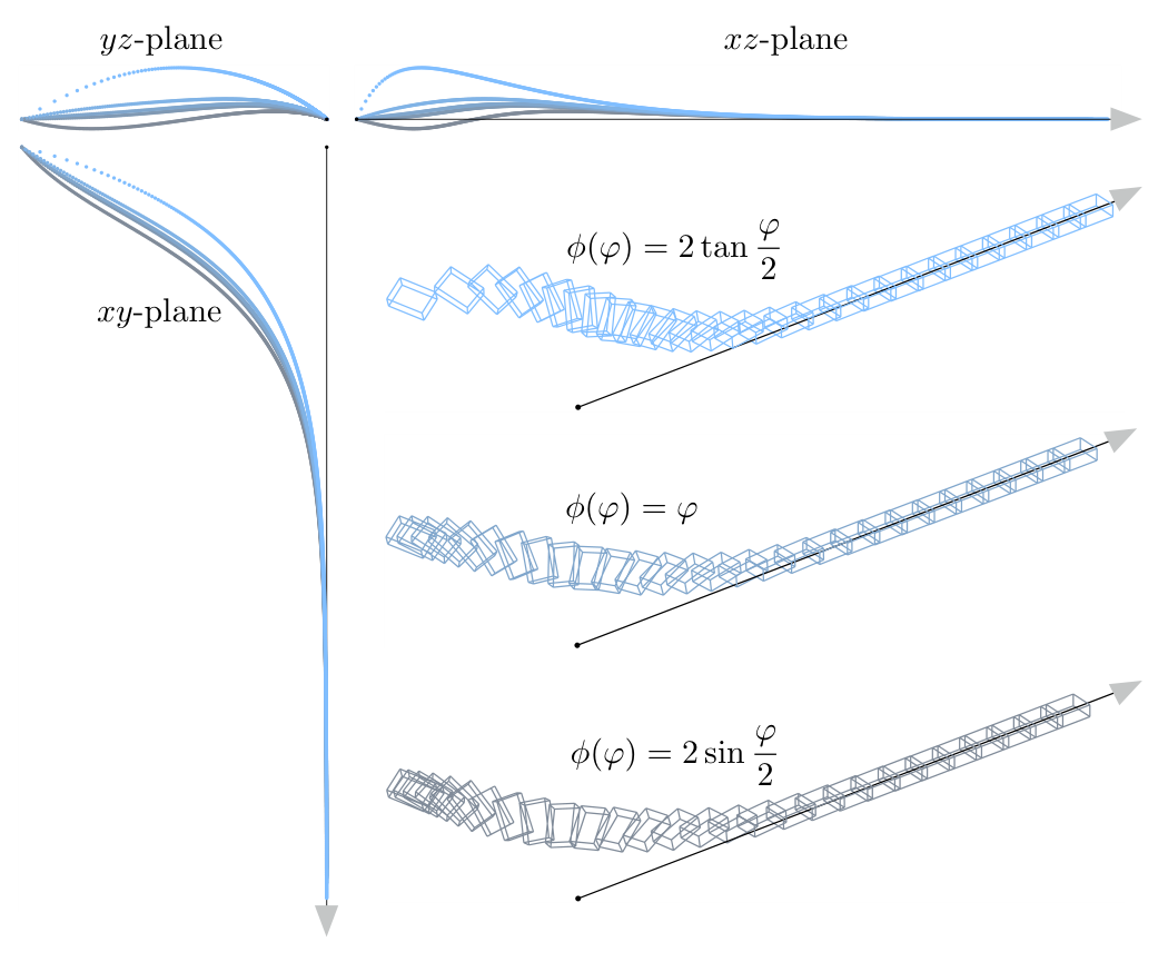
Pose interpolation has been discussed extensively in the literature; Han and Bauchau 2016, Han and Bauchau 2018 provide some representative examples. Here our goal is not to claim a new method of pose interpolation but rather to show the effect of simply changing the generating function on a basic interpolation scheme defined in the vectorspace.

We can define a ‘linear’ interpolation scheme for poses using any of our vector parameterizations:

where ${\bm{\xi}}_{\rm initial}$ is an initial pose, ${\bm{\xi}}_{\rm final}$ a final pose, and $s\in[0,1]$ the interpolation variable. As we vary $s$ from $0$ to $1$, the vector, ${\bm{\xi}}$ will vary and so too will $\mathbf{T}({\bm{\xi}})$. This allows the smooth transition from one pose to another.

Figure 2 provides a qualitative example of this scheme for all five generating functions, $\phi(\varphi)$, listed in Table 1 with $\mathbf{D}({\bm{\phi}})=\mathbf{J}({\bm{\phi}})$. The paths taken each correspond to a geodesic in $\mathbb{R}^{6}$, but when mapped to $SE(3)$ are quite different. Notably, none of the paths are straight lines in Euclidean space owing to the coupling between translation and rotation. As the rotational motion becomes smaller, the paths followed by the different generating functions look more similar owing to (17). Looking more closely at Figure 2, we can also observe that the spacing of the steps are quite different for the different generating functions, even though we stepped $s$ uniformly. The $\tan$ generating functions take larger steps at the beginning but smaller ones at the end, while the $\sin$ ones do the opposite, and the $\phi(\varphi)=\varphi$ function keeps the steps even throughout. Naturally, we can make the steps in the interpolation variable, $s$, as small as we like to obtain smooth interpolation; we chose fairly large steps to keep the plot in Figure 2 from becoming too cluttered.

Pose servoing is also a well studied topic. Here we simply want to show the effect of changing the pose mapping on a simple control law defined in the vectorspace. We define a ‘linear’ control law to servo onto a reference path. Consider a reference pose, $\mathbf{T}_{\rm ref}$, that we want to track. We can compare our current pose, $\mathbf{T}({\bm{\xi}})$, to this reference and put it through the inverse mapping to create an ‘error vector’:

where the left arrow stands in for the inverse of any of our pose mappings. We can then adjust our pose to be slightly closer to the reference pose (which is moving) using a simple control law:

with $\kappa>0$ a gain. As the error ${\bm{\xi}}_{\rm error}$ approaches zero, the moving pose, $\mathbf{T}({\bm{\xi}})$ will approach the reference pose, $\mathbf{T}_{\rm ref}$.

Figure 3 provides an example of servoing to a reference pose that is moving straight along the $x$-axis, starting from a poor initial pose that is translated and rotated from the reference. We kept the vector control law (including the gain) identical and varied only the choice of pose mapping. As expected, we see different transient behaviour resulting from the different pose mappings as they seek the reference.

We use this section to discuss aligning two clouds of three-dimensional points. Our problem is similar to that of Barfoot et al. 2011, but formulated directly on $SE(3)$.

References

- Ball [1900] Ball, R. S., A Treatise on the Theory of Screws, Cambridge university press, 1900.
- Barfoot [2017] Barfoot, T. D., State Estimation for Robotics, Cambridge University Press, 2017.
- Barfoot et al. [2011] Barfoot, T. D., Forbes, J. R., and Furgale, P. T., “Pose Estimation using Linearized Rotations and Quaternion Algebra,” Acta Astronautica, 68(1-2):101–112, 2011.
- Barfoot and Furgale [2014] Barfoot, T. D. and Furgale, P. T., “Associating Uncertainty with Three-Dimensional Poses for use in Estimation Problems,” IEEE Transactions on Robotics, 30(3):679–693, 2014, (code).
- Bauchau [2011] Bauchau, O. A., Flexible multibody dynamics, Springer Science & Business Media, 2011.
- Bauchau and Choi [2003] Bauchau, O. A. and Choi, J.-Y., “The vector parameterization of motion,” Nonlinear Dynamics, 33(2):165–188, 2003.
- Bauchau and Li [2011] Bauchau, O. A. and Li, L., “Tensorial parameterization of rotation and motion,” Journal of computational and nonlinear dynamics, 6(3), 2011.
- Bauchau and Trainelli [2003] Bauchau, O. A. and Trainelli, L., “The vectorial parameterization of rotation,” Nonlinear dynamics, 32(1):71–92, 2003.
- Borri et al. [2000] Borri, M., Trainelli, L., and Bottasso, C. L., “On representations and parameterizations of motion,” Multibody System Dynamics, 4(2):129–193, 2000.
- Cayley [1846] Cayley, A., “Sur quelques propriétés des déterminants gauches.” Journal für die reine und angewandte Mathematik, 1846(32):119–123, 1846.
- Chasles [1830] Chasles, M., “Note sur les propriétés générales du système de deux corps semblables entr’eux et placés d’une manière quelconque dans l’espace; et sur le déplacement fini ou infiniment petit d’un corps solide libre,” Bulletin des Sciences Mathématiques, Férussac, 14:321–26, 1830.
- Chirikjian [2009] Chirikjian, G. S., Stochastic Models, Information Theory, and Lie Groups: Classical Results and Geometric Methods, volume 1-2, Birkhauser, New York, 2009.
- Condurache and Ciureanu [2020] Condurache, D. and Ciureanu, I.-A., “Baker–Campbell–Hausdorff–Dynkin Formula for the Lie Algebra of Rigid Body Displacements,” Mathematics, 8(7):1185, 2020.
- D’Eleuterio and Barfoot [2021] D’Eleuterio, G. M. T. and Barfoot, T. D., “On the Eigenstructure of Rotations and Poses: Commonalities and Peculiarities,” 2021, in preparation for submission.
- Han and Bauchau [2016] Han, S. and Bauchau, O. A., “Manipulation of motion via dual entities,” Nonlinear Dynamics, 85(1):509–524, 2016.
- Han and Bauchau [2018] Han, S. and Bauchau, O. A., “On the global interpolation of motion,” Computer Methods in Applied Mechanics and Engineering, 337:352–386, 2018.
- Hughes [1986] Hughes, P. C., Spacecraft attitude dynamics, John Wiley and Sons, New York, 1986.
- Junkins et al. [2011] Junkins, J. L., Majji, M., Macomber, B., Davis, J., Doebbler, J., and Nosterk, R., “Small Body Proximity Sensing with a Novel HD 3D Ladar System,” Advances in the Astronautical Sciences, 141:341–354, 2011.
- Maimone et al. [2007] Maimone, M., Cheng, Y., and Matthies, L., “Two years of visual odometry on the mars exploration rovers,” Journal of Field Robotics, 24(3):169–186, 2007.
- Majji et al. [2011] Majji, M., Davis, J., Doebbler, J., Junkins, J., Macomber, B., Vavrina, M., and Vian, J., “Terrain mapping and landing operations using vision based navigation systems,” in AIAA Guidance, Navigation, and Control Conference, page 6581, 2011.
- Matthies and Shafer [1987] Matthies, L. and Shafer, S., “Error modeling in stereo navigation,” IEEE Journal on Robotics and Automation, 3(3):239–248, 1987.
- Mortari et al. [2007] Mortari, D., Markley, F. L., and Singla, P., “Optimal linear attitude estimator,” Journal of Guidance, Control, and Dynamics, 30(6):1619–1627, 2007.
- Mozzi [1763] Mozzi, G., Discorso matematico sopra il rotamento momentaneo dei corpi, Donate Campo, 1763.
- Murray et al. [1994] Murray, R. M., Li, Z., and Sastry, S., A Mathematical Introduction to Robotic Manipulation, CRC Press, 1994.
- Qian et al. [2020] Qian, D., Charland-Arcand, G., and Forbes, J. R., “TWOLATE: Total Registration of Point-Clouds Using a Weighted Optimal Linear Attitude and Translation Estimator,” in 2020 IEEE Conference on Control Technology and Applications (CCTA), pages 43–48, IEEE, 2020.
- Selig [2007] Selig, J. M., “Cayley maps for SE(3),” in 12th International Federation for the Promotion of Mechanism and Machine Science World Congress, page 6, London South Bank University, 2007.
- Stuelpnagel [1964] Stuelpnagel, J., “On the parametrization of the three-dimensional rotation group,” SIAM review, 6(4):422–430, 1964.
- Wong and Majji [2016] Wong, X. I. and Majji, M., “A structured light system for relative navigation applications,” IEEE Sensors Journal, 16(17):6662–6679, 2016.
- Wong et al. [2018] Wong, X. I., Singla, P., Lee, T., and Majji, M., “Optimal Linear Attitude Estimator for Alignment of Point Clouds,” in 2018 IEEE/CVF Conference on Computer Vision and Pattern Recognition Workshops (CVPRW), pages 1577–15778, IEEE, 2018.
- Yang et al. [2020] Yang, H., Shi, J., and Carlone, L., “Teaser: Fast and certifiable point cloud registration,” IEEE Transactions on Robotics, 37(2):314–333, 2020.