Contact-line deposits from multiple evaporating droplets
Abstract
Building on the recent theoretical work of Wray et al. [J. Fluid Mech. 884, A45 (2020)] concerning the competitive diffusion-limited evaporation of multiple thin sessile droplets in proximity to each other, we obtain theoretical predictions for the spatially non-uniform densities of the contact-line deposits (often referred to as “coffee stains” or “ring stains”) left on the substrate after such droplets containing suspended solid particles have completely evaporated. Neighbouring droplets interact via their vapour fields, which results in a spatially non-uniform “shielding” effect. We give predictions for the deposits from a pair of identical droplets, which show that the deposit is reduced the most where the droplets are closest together, and demonstrate excellent quantitative agreement with experimental results of Pradhan and Panigrahi [Coll. Surf. A 482, 562–567 (2015)]. We also give corresponding predictions for a triplet of identical droplets arranged in an equilateral triangle, which show that the effect of shielding on the deposit is more subtle in this case.
Keywords:
Droplets, Evaporation, Particles, Contact-Line Deposits, Coffee Stains, Ring Stains, Shielding EffectI Introduction
The evaporation of sessile droplets has been the subject of extensive experimental, numerical and analytical investigation in recent years (see, for example, (Routh 2013; Larson 2014; Stauber et al. 2014; Brutin and Starov 2018; Giorgiutti-Dauphiné and Pauchard 2018), and the references therein), partly motivated by the wide range of everyday and industrial situations, such as protein crystallography (Dimitrov et al. 1994), surface patterning (Boneberg et al. 1997), ink-jet printing, including that of OLED displays (Bale et al. 2006), and agrochemical spraying of plants (Tredenick et al. 2021), in which it occurs.
Particular attention has been paid to the so-called “coffee-stain” or “ring-stain” effect: when a droplet of coffee (or indeed a droplet of any fluid containing suspended solid particles) with a pinned (i.e. a fixed) contact line evaporates it tends to deposit the majority of the particles close to the location of its contact line, even if the particles were initially distributed uniformly throughout the bulk of the droplet. The explanation of this phenomenon, as first given by Deegan et al. 1997, is that as the droplet evaporates its free surface adjusts quasi-statically under the effect of capillarity, inducing a flow within the droplet that advects the particles suspended within it towards its contact line, resulting in a characteristic ring-like contact-line deposit on the substrate after the droplet has completely evaporated. Since the seminal work by Deegan et al. 1997, many aspects of this phenomenon have been investigated in considerable detail (see, for example, (Deegan 2000; Deegan et al. 2000; Popov 2005; Zheng 2009; Askounis et al. 2011; Hamamoto et al. 2011; Marín et al. 2011a; Marín et al. 2011b; Yunker et al. 2011; Berteloot et al. 2012; Askounis et al. 2013; Wray et al. 2014; Boulogne et al. 2016; Kang et al. 2016; Kim and Weon 2018) and the reviews (Larson 2014; Mampallil and Eral 2018; Yang et al. 2021)). Note that although Deegan et al. 1997 considered the most commonly studied situation of diffusion-limited evaporation into a quiescent atmosphere with a uniform far-field concentration of vapour, which has a large (theoretically singular) evaporative flux close to the contact line, the effect is quite robust, and even, for example, a spatially uniform evaporative flux will lead to advection of particles towards the contact line (see, for example, (Deegan et al. 2000; Zheng 2009; Boulogne et al. 2016)).
The vast majority of the previous work on deposition from evaporating sessile droplets has, for obvious reasons, focused on axisymmetric deposits from axisymmetric droplets. There has, however, been some work on non-axisymmetric deposits from non-axisymmetric droplets (see, for example, (Deegan et al. 1997; Cheng et al. 2008; Du and Deegan 2015; Kim et al. 2017; Sáenz et al. 2017; Timm et al. 2019; Tredenick et al. 2021)). In particular, Du and Deegan 2015 examined a two-dimensional droplet on an inclined substrate numerically, and found that, depending on the initial volume of the droplet and the angle of inclination of the substrate, the larger deposit can occur at either the upper or the lower contact line, while Sáenz et al. 2017 investigated a variety of non-axisymmetric droplets both experimentally and numerically, and found that larger deposits occur where the contact line has the largest curvature (e.g. near the tips of a droplet with a triangular contact line). However, their theoretical modelling of the density of the deposit was essentially phenomenological.
Non-axisymmetric deposits also occur as a result of the non-axisymmetric evaporation of multiple droplets in proximity to each other, a situation that occurs much more commonly in practice than single droplets in isolation (Bale et al. 2006). Specifically, neighbouring droplets undergoing diffusion-limited evaporation interact via their vapour fields, which results in a spatially non-uniform “shielding” effect that reduces the evaporation rate. While there have been some analytical studies of mathematically analogous situations concerning clusters of micro-contacts and nanobubbles (see, for example, (Argatov 2011; Dollet and Lohse 2016)), analytical work on the evaporation of multiple droplets is rather limited. To a large extent this is explained by the inherent difficulty of analysing such situations, and while the evaporation of multiple droplets in various configurations has been the subject of growing recent interest (see, for example, (Lacasta et al. 1998; Schäfle et al. 1999; Deegan et al. 2000; Kokalj et al. 2010; Sokuler et al. 2010; Pradhan and Panigrahi 2015; Carrier et al. 2016; Castanet et al. 2016; Shaikeea and Basu 2016; Shaikeea et al. 2016; Hatte et al. 2019; Khilifi et al. 2019; Pandey et al. 2020; Schofield et al. 2020; Wray et al. 2020)), the previous studies have been predominantly numerical or experimental. Two notable exceptions are the recent work of Wray et al. 2020, who, building on the earlier work of Fabrikant 1985 concerning a model for diffusion through a porous membrane, analysed the spatially non-uniform shielding that occurs in arbitrary configurations of thin droplets with circular contact lines, and that of Schofield et al. 2020, who used conformal-mapping techniques to analyse the analogous spatially non-uniform shielding that occurs in the closely related two-dimensional situation of a pair of evaporating ridges. In particular, Wray et al. 2020 gave explicit formulae for the evaporative flux of arbitrary configurations of droplets that were found to be remarkably accurate up to and including the limit of touching droplets, and led to theoretical predictions for the evolution of an arrangement of seven droplets that were found to be in excellent agreement with experimental results of Khilifi et al. 2019.
In the present contribution we build on the work of Wray et al. 2020 in order to analyse the spatially non-uniform densities of the deposits left on the substrate by the diffusion-limited evaporation of multiple thin droplets with pinned circular contact lines in proximity to each other. Specifically, in Secs. II and III we formulate and solve the evaporation, hydrodynamic, and particle-transport problems. In Sec. IV we give theoretical predictions for the densities of the deposits from a pair of identical droplets, and demonstrate excellent quantitative agreement with experimental results of Pradhan and Panigrahi 2015. In Sec. V we also give corresponding predictions for a triplet of identical droplets arranged in an equilateral triangle. Finally, we summarise our conclusions in Sec. VI.
The present analysis is for the most commonly studied case of small droplets, in which capillary effects dominate over gravitational effects, corresponding to the limit of small Bond number. In Appendix A we describe the corresponding analysis for the less commonly studied case of large droplets, corresponding to the limit of large Bond number, in which even greater analytical progress is possible.
II Problem Formulation
 |
| (a) |
 |
| (b) |
Consider () thin axisymmetric sessile droplets with pinned circular contact lines with constant radii and fixed centres at for on a planar solid substrate , as shown in Fig. 1(a). The droplets undergo quasi-static diffusion-limited evaporation, which, as described in Sec. I, induces flows within the droplets that advect the solid particles suspended within them towards their contact lines. The goal of the present work is to determine the spatially non-uniform densities of the deposits left on the substrate after the droplets have completely evaporated. Three coupled problems must therefore be solved: the evaporation problem for the concentration of vapour in the atmosphere (which determines the rates of evaporation of the droplets), the hydrodynamic problem for the fluid flow that is induced in each droplet, and the advection problem for the motion of the particles suspended within each droplet, as shown in Fig. 1(b). We now discuss each of these problems in turn.
II.1 The evaporation problem
According to the diffusion-limited model, the quasi-static concentration of vapour in the atmosphere, denoted by , satisfies Laplace’s equation subject to conditions of complete saturation at the free surfaces of the droplets and of no flux of vapour through the unwetted part of the substrate. Following Wray et al. 2020, we scale and nondimensionalise variables appropriately for the atmosphere according to
where and are Cartesian coordinates in the plane , , and are local polar coordinates with their origin at the centre of the droplet, is a characteristic radius of the contact lines of the droplets, is the constant diffusion coefficient of vapour in the atmosphere, and are the constant saturation concentration and far-field concentration of vapour, and and are the local evaporative flux and the integral evaporative flux from the droplet, respectively, which are related by
| (3) |
where denotes the free surface of the droplet. Since the contact lines of the droplets are pinned, and are independent of time except for discontinuous jumps when any droplet completely evaporates; in particular, and jump instantaneously to zero when the droplet completely evaporates.
For clarity, we immediately drop the star superscripts on non-dimensional quantities, and so the boundary conditions on become on for , on the unwetted part of the substrate , and the far-field condition as .
As Wray et al. 2020 described, the earlier work of Fabrikant 1985 on diffusion through a porous membrane, when interpreted in terms of the evaporation of multiple thin sessile droplets, shows that the integral evaporative flux is given, to a high degree of accuracy, by the solution of the linear system
| (4) |
where () is the distance between the centres of the and the droplets shown in Fig. 1(a) and given by
| (5) |
Wray et al. 2020 also showed that, to the same high degree of accuracy, the local evaporative flux is given by
| (6) |
where
| (7) |
is the local evaporative flux from the droplet in isolation, and is the angle between the axis and the line joining the centres of the and the droplets, also shown in Fig. 1(a) and given by
| (8) |
II.2 The hydrodynamic problem
The velocity and pressure within the droplet, denoted by and , where denotes time, satisfy the usual mass-conservation and Stokes equations subject to the usual boundary conditions, and the free surface, contact angle and volume of the droplet are denoted by , () and , respectively.
We scale and nondimensionalise variables appropriately for the droplet according to
in which () is a characteristic contact angle of the droplets, is the constant coefficient of surface tension of the fluid, is the constant atmospheric pressure, and and are a characteristic time for the evaporation and a characteristic velocity, defined by
| (11) |
respectively, where is the constant density of the fluid.
At leading order in the governing equations for the droplet are, with the hats dropped for clarity,
| (12) |
where is an appropriate capillary number, defined by
| (13) |
where is the constant viscosity of the fluid. Equation (12) is to be solved subject to zero velocity at the substrate,
| (14) |
balances of normal and tangential stress at the free surface of the droplet,
| (15) |
and the kinematic condition,
| (16) |
where and , defined by
| (17) |
are the local radial and azimuthal volume fluxes of fluid within the droplet.
We consider the situation in which capillary effects are strong, corresponding to small values of the capillary number , and so we seek asymptotic solutions of the form
| (18) |
in the limit . As we shall see, for the analysis of particle transport presented in Sec. II.3, we require only the leading order velocity components and , which in turn require and .
At leading order in , equations (12) and (15) show that the leading-order pressure is independent of , and , and is given by , and the leading-order free surface takes the familiar paraboloidal form
| (19) |
The leading-order volume of the droplet is therefore given by
| (20) |
At first order in , equations (12), (15) and (14) lead to
| (21) |
and so the leading-order local fluid fluxes (17) are
| (22) |
Dropping the subscript “1” on henceforth for clarity, the kinematic condition (16) therefore gives
| (23) |
We may use this condition to obtain the differential equation satisfied by by noting that is independent of the azimuthal coordinate , and that, by global mass conservation, the volume satisfies
| (24) |
so that, with (19) and (20), may be written as
| (25) |
Finally, therefore, the kinematic condition (23) may be expressed in the form
| (26) |
which is a partial differential equation for , with all of the other quantities in (26) being known. Once is determined from (26), the local fluid fluxes and are given by (22).
The depth-averaged radial and azimuthal velocities, denoted by and , are defined by
| (27) |
respectively. For future reference, note that the streamlines of the depth-averaged flow are determined by solving
| (28) |
Since and have the same functional dependence on , the has cancelled out of (28), and so the streamlines depend on time only via changes in the flux . This means that in certain situations the computation of the streamlines is simplified somewhat by the fact (mentioned earlier) that and hence are independent of except for discontinuous jumps when any droplet completely evaporates. Specifically, if the droplets are arranged in such a way that all of them completely evaporate at exactly the same time then their streamlines remain unchanged throughout the evaporation. In this case the determination of the density of the deposit reduces to performing a single integral, as will be described in Sec. IV.2 below.
II.3 The particle-transport problem
The motion of the particles suspended within each droplet is due to a combination of advection by the flow and diffusion, and so the concentration of particles in the droplet, denoted by , satisfies the (scaled) advection–diffusion equation
| (29) |
in which has been nondimensionalised according to , where is a characteristic concentration of particles, is an appropriate Péclet number, and is the constant diffusion coefficient for the particles in the fluid, and where the star subscript has again been dropped for clarity. Equation (29) is subject to conditions of no flux of particles through either the free surface of the droplet or the substrate,
| (30) |
where denotes the outward unit normal to the free surface of the droplet.
As is well known (see, for example, Wray et al. 2014), when the Péclet number is such that , the leading-order concentration of particles, , is independent of and satisfies
| (31) |
where the depth-averaged radial and azimuthal velocities and are given by (27). Equation (31) may be solved by the method of characteristics:
| (32) |
subject to a prescribed initial condition at . For simplicity, in all of the results presented below we assume that the initial concentration of particles takes the same uniform value in all of the droplets, which we may, without loss of generality, take to be unity.
III Solution for the pressure
In general, the expression for the evaporative flux given in (6) is rather complicated, and precludes solving (26) for the pressure in closed form; however, we may determine to arbitrary accuracy as follows.
For we expand given by (6) as the convergent series
| (33) |
which we may rearrange in the form of a truncated Fourier series
| (34) |
for a chosen number of modes (), with known functions and . To determine we decompose it into a corresponding form, namely
| (35) |
substitution of which into (26) leads to a sequence of differential equations for and ,
| (36) |
and
| (37) |
Equation (36) may be solved directly (up to an irrelevant additive constant) subject to regularity at the origin. Equation (37) may be solved by the method of variation of parameters. Specifically, the homogeneous version of (37), namely
| (38) |
has solutions and given by
| (39) |
which satisfies
| (40) |
and
| (41) |
which satisfies
| (42) |
where , and so the solution of the inhomogeneous equation (37) is
| (43) |
where
| (44) |
is the Wronskian, which can be evaluated to give
| (45) |
Note that we have chosen the forms of the homogeneous solutions and imposed the boundary conditions by selecting the lower limits of the integrals in equation (43) so as to ensure regularity at the origin (first integral) and at the contact line (second integral). In general, the integrals in equation (43) must be evaluated numerically to obtain . Note, however, that, as described in Appendix A, even greater analytical progress is possible for the corresponding problem in the limit of large Bond number.
IV A pair of identical droplets
In this Section we apply the general methodology developed in Secs. II and III to determine the densities of the deposits from a pair of identical droplets, a situation for which the predictions of the present asymptotic theory for the local evaporative flux and the integral evaporative flux were validated by Wray et al. 2020. In Sec. IV.1 we determine the local evaporative fluxes, the fluid fluxes and the resulting streamlines of the depth-averaged flows, in Sec. IV.2 we determine the density of the deposit, while in Sec. IV.3 we compare the theoretical predictions for the density of the deposit with the experimental results of Pradhan and Panigrahi 2015.
IV.1 Evaporative fluxes, fluid fluxes and streamlines


Consider the evaporation of a pair of identical droplets, which we may, without loss of generality, take to be of unit radius , with their centres located at , i.e. with their centres a distance apart. As Wray et al. 2020 showed, the two droplets have the same integral evaporative flux given by , where
| (46) |
By symmetry, it is sufficient to consider only the left-hand droplet with its centre located at , corresponding to . The local evaporative flux from the surface of the droplet is given by
| (47) |
which may be expanded as
| (48) |
where
| (49) |
and
| (50) |
is the flux from the same droplet in isolation. The expansion (48) with (49) can then be used to determine the pressure in (35), and thus the local fluid fluxes and in (22). Figure 2 shows contours of the local evaporative fluxes (left-hand droplet) and (right-hand droplet), and the resulting streamlines of the depth-averaged flows for , with the expansion (48) truncated after Fourier modes. Figure 2 illustrates how the shielding effect reduces the local evaporative flux the most where the droplets are closest together (i.e. at ) and the least where they are furthest apart (i.e. at ) Wray et al. 2020. For an isolated droplet the contours of given by (50) are concentric circles and the streamlines are radial lines; Fig. 2 also illustrates how the shielding effect skews both of them towards the other droplet.
IV.2 Density of the deposit
(a)
(b)

We now determine the density of the deposit resulting from the evaporation of the droplets. By symmetry, the two droplets completely evaporate at the same time, and so the streamlines of their depth-averaged flows remain unchanged throughout the evaporation and, as in Sec. IV.1, it is sufficient to consider only the left-hand droplet with its centre located at .
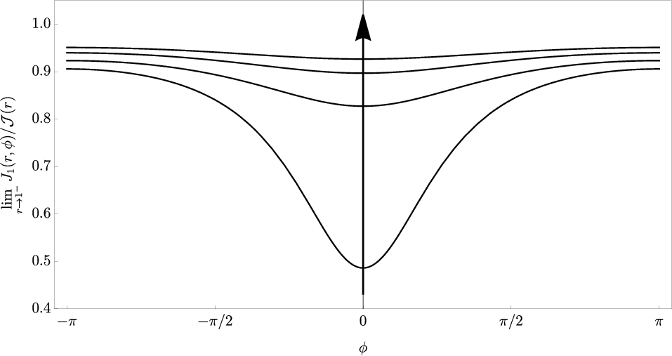
We work relative to (non-orthogonal) curvilinear co-ordinates defined by the streamlines with their origin at the “source” from which all of the streamlines of the depth-averaged flow emanate, denoted by , shown in Fig. 2. Note that, contrary to what Fig. 2 may suggest, the source from which the streamlines emanate, , does not, in general, coincide exactly with the location of the minimum of the local evaporative flux. The difference between the two is readily evident in Fig. 6 which appears subsequently in Sec. V. The coordinate parameterises the streamlines such that the local behaviour of the streamlines near the source is given by as , while the coordinate is the arc length along each streamline, measuring from at the source to at the contact line. Note that is therefore the length of the streamline parameterised by from the source to the contact line.
Since the fluid flow always advects the particles along the streamlines towards the contact line, the mass of the deposit that eventually accumulates at the contact line between the point with coordinate and a general point with coordinate , denoted by , is exactly equal to the mass of particles originally in the curved sector between the streamlines parameterised by and by , i.e.
| (51) |
Note that, by definition, and . Once has been determined, the density of the deposit at a point on the contact line with polar angle , denoted by , is then given by
| (52) |
Figure 3 shows the evaporative flux at the contact line normalised by the corresponding flux for the same droplet in isolation, , and the density of the deposit as functions of the azimuthal coordinate for several values of . In particular, Fig. 3(b) shows that the shielding effect described in Sec. IV.1 and shown in Fig. 2 leads to a spatially non-uniform deposit with the smallest density where the shielding effect is strongest (i.e. at ) and the largest density where it is weakest (i.e. at ). Note that, by conservation of mass, the total mass of the deposit is the same for all of the values of used in Fig. 3(b).
IV.3 Comparison with experimental results

In general, comparing theoretical predictions for the density of a deposit with experimentally obtained images of deposition patterns is a challenging task. In particular, because the depth of the deposit cannot usually be readily determined from images taken from above the droplet, obtaining a quantitative measure of the amount of deposit from experimental images may often not be possible due to saturation and non-linearity of the data. For example, in Fig. 2 of Pradhan and Panigrahi 2015, reproduced here as Fig. 4, the image of the final deposition pattern from a pair of similar droplets of water containing 1 m particles shown in part (d) has zero transmittance through the contact-line deposit, making it impossible to quantify its spatial distribution. However, the image of the final deposition pattern from a pair of similar droplets of ink shown in part (b) has nonzero transmittance throughout the vast majority of the contact-line deposit, and so offers us an opportunity to quantify the relative amount of deposit as a function of azimuthal position.
In order to compare the results of Pradhan and Panigrahi 2015 with the present theoretical predictions, it is first necessary to convert the information contained within the image into a form proportional to the density distribution . The raw data extracted from the image corresponds to the reflectance of the deposit; this must be converted into its absorbance, which can then be related to its concentration via the Beer–Lambert law (Swinehart 1962),
| (53) |
where is the absorbance, is the radiant power (reflectance) or intensity of the light as measured at each pixel in the image, is the initial radiant power of the light before absorbance, is the molar absorptivity of the deposit (which may reasonably be assumed to be constant), is the path length of the light in the deposit, and is the concentration of the absorbing species. The values for are known, as this is the light gathered by each pixel in the sensor of the camera to generate the image; however, the value of is unknown. (Ideally would have been determined through the collection of a reference image in which the light reflected from a calibrated sample, such as a 99% reflectance standard, was captured.) Therefore, it is necessary to make an estimate of , and to do this we used the maximum possible brightness value of as the reference value for all of the pixels (consistent with the brightness of the image outside the footprint of the droplets). In order to gather only density data from the deposit near the contact line of each droplet, and not the density of any residual deposit left within it, the data was taken from an annular region around the edge of the footprint of each droplet. Slightly unfortunately, as Fig. 4 shows, in the published image the deposit from the left-hand droplet is overlaid by the head of an arrow that the authors added to indicate the region of weakest deposition. In order to reduce artifacts associated with this arrowhead, it was removed from the data by interpolating from the neighbouring pixels. The procedure for the extraction of the data for each droplet was implemented in Python van Rossum 1995, and is detailed below:
- 1.
Convert the image to binary, and determine its centre of mass.
- 2.
Trace out the outer perimeter of the deposit.
- 3.
Define a second inner perimeter at of the radius of the outer perimeter measured relative to the centre of mass.
- 4.
Divide the annular region between the inner and outer perimeters into sectors subtending equal angles at the centre of mass. In practice, sectors were used.
- 5.
Use the Beer–Lambert law (53) to calculate the absorbance of each pixel, which is proportional to the mass of residue per unit area.
- 6.
Integrate the mass per unit area numerically over each sector, and divide by the angle subtended, to determine the corresponding proportional mass per unit length of the contact line (i.e. the density to be compared with ).
(a)
 |
(b)
 |
The constant of proportionality for comparison with is determined by imposing the condition that the integral of the density is , in line with the nondimensionalisation in Sec. II.3. Figure 5 shows a comparison between the present theoretical predictions and the experimental results extracted from Fig. 2(b) of Pradhan and Panigrahi 2015 using the procedure described above. Specifically, Fig. 5(a) compares the density of the deposit predicted by (52) (shown with the black solid curve) with the experimental results for the left-hand droplet (shown with the blue dashed curve) and the right-hand droplet (shown with the red dotted curve). Given the approximations made in both the mathematical model and in the processing of the experimental image, the agreement between theory and experiment shown in Fig. 5(a) is remarkably good, especially when it is noted that no fitting parameters have been used. The only scaling used is to ensure that the total mass (not given by Pradhan and Panigrahi 2015) is the same for theory and experiment.
While the agreement between theory and experiment shown in Fig. 5(a) is already good, with an integral absolute relative error of around 7% for the left-land droplet and 9% for the right-hand droplet, the experimental results are inevitably rather noisy. Figure 5(b) compares the density of the deposit predicted by (52) (shown again with the black solid curve) with the experimental results averaged across both droplets, as well as about (shown with the black dashed curve). In particular, Fig. 5(b) shows that, as expected, averaging reduces the noise in the experimental results and, rather pleasingly, leads to even better agreement between theory and experiment than that shown in Fig. 5(a), with an integral absolute relative error of around 3%. Figure 5(b) also includes the corresponding phenomenological estimate of the radially-integrated fluid flux (now interpreted as the density of the deposit) derived by Wray et al. 2020 by using the approach of Sáenz et al. 2017, denoted here by , given by
| (54) |
which can be evaluated to yield
| (55) |
where and is given by (46). In particular, Fig. 5(b) shows that the estimate (55) is reasonably accurate, with an integral absolute relative error of around 9%, and captures the experimental results qualitatively but not quite quantitatively.
V A triplet of identical droplets


(a)
(b)

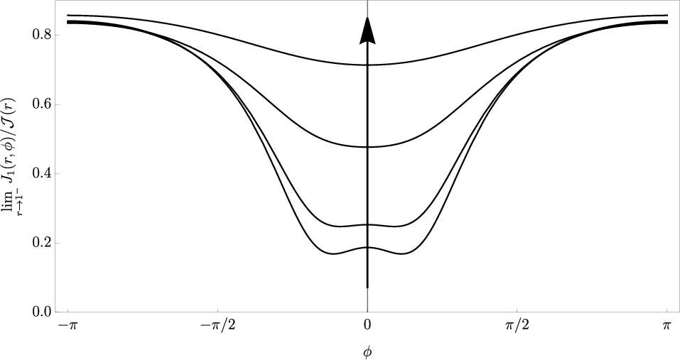
In this Section we use the same approach as that described in Sec. IV to determine the densities of the deposits from a triplet of identical droplets of unit radius with their centres located at and , i.e. with their centres a distance apart. Note that, in the terminology used by Wray et al. 2020, the centres of the droplets lie at the vertices of an equilateral triangle with side and circumradius . Similarly to in Sec. II, by symmetry it is sufficient to consider only the left-most droplet with its centre located at , corresponding to . The results are summarised in Figs. 6 and 7, which show contours of the local evaporative fluxes for and the resulting streamlines of the depth-averaged flows for , and the normalised evaporative flux at the contact line, , and the density of the deposit as functions of the azimuthal coordinate for several values of , respectively. In particular, Figs. 6 and 7 show that, as expected, the shielding effect again reduces the local evaporative flux and leads to a spatially non-uniform deposit at the contact line. However, in this case the effect is evidently more subtle than that described in Sec. IV for a pair of droplets. Specifically, when the droplets are sufficiently far apart, the shielding effect reduces the local evaporative flux the most in the direction towards the centre of the triangle (i.e. at ) and the least in the direction away from the centre of the triangle (i.e. at ), but these directions do not now correspond to those in which the droplets are closest together (i.e. at ). However, when the droplets are sufficiently close together, the local evaporative flux develops two (symmetric) local minima at non-zero values of (as shown by the curve for in Fig. 7(a)), and the density of the deposit develops local maxima and mimima (as shown by the curve for in Fig. 7(b)). Note that, as in Fig. 3(b), by conservation of mass, the total mass of the deposit is the same for all of the values of used in Fig. 7(b).
VI Conclusions
In the present work we obtained theoretical predictions for the spatially non-uniform densities of the contact-line deposits left on the substrate after the competitive diffusion-limited evaporation of multiple thin axisymmetric sessile droplets in proximity to each other. In particular, we gave predictions for the deposits from a pair of identical droplets, which showed that the deposit is reduced the most where the droplets are closest together, and demonstrated excellent quantitative agreement with experimental results of Pradhan and Panigrahi 2015. We also gave corresponding predictions for a triplet of identical droplets arranged in an equilateral triangle, which showed that the effect of shielding on the deposit is more subtle in this case.
We note that, while the present analysis is formally restricted to thin droplets, the fact that much of the deposition from a non-thin droplet occurs towards the end of its lifetime when the contact angle is small and the velocity within the droplet is large (sometime referred to as “the rush hour”, see, for example, (Hamamoto et al. 2011; Marín et al. 2011b)) means that the results of the present analysis are also expected to provide useful predictions for the contact-line deposits from non-thin droplets.
A brief observation about the validity of the diffusion-limited model of evaporation is perhaps appropriate here. The excellent agreement with experimental results of Khilifi et al. 2019 found by Wray et al. 2020 attests to the accuracy of the theoretical predictions for the integral evaporative flux, but it does not tell us anything directly about the accuracy of the theoretical predictions for the spatial distribution of the local evaporative flux or the resulting fluid flow within the droplet. For an isolated axisymmetric droplet, the fluid flow within the droplet is axisymmetric and the density of the deposit depends only on the initial distribution of particles and so, in particular, the density of the deposit does not depend on the details of the fluid flow. However, in non-axisymmetric situations, such as the non-axisymmetric droplets considered by Sáenz et al. 2017 and the non-axisymmetric evaporation of multiple droplets considered in the present work, understanding the details of the fluid flow is essential to determining the density of the deposit. Thus the comparison with experimental results described in the present work is perhaps the most stringent test of the diffusion-limited model to date, a test which it evidently passes remarkably well.
Finally, we note that the approach described in the present work is rather general and can, in principle, be applied to any arrangement of any number of thin droplets with pinned or unpinned contact lines.
Acknowledgements
The authors gratefully acknowledge valuable discussions with Hannah-May D’Ambrosio (University of Strathclyde) and Prof. Khellil Sefiane (University of Edinburgh) about various aspects of droplet evaporation.
Appendix A Solution in the limit of large Bond number
As mentioned at the end of Sec. I, the present analysis is for the most commonly studied case of small droplets in which capillary effects dominate over gravitational effects, corresponding to the limit of small Bond number. In this Appendix we describe the corresponding analysis in the case of large droplets, for which gravitational effects dominate over capillary effects, corresponding to the limit of large Bond number, in which even greater analytical progress is possible.
In the limit of large Bond number, the free surface of the droplet is flat, i.e. , except in a narrow region near the contact line which we may neglect (Rienstra 1990), and so the volume of the (nearly cylindrical) droplet is now given by . The local fluid fluxes are again given by (17), while the kinematic condition (23) simplifies to
| (A.56) |
and hence (25) becomes
| (A.57) |
and so the partial differential equation for given by (26) becomes
| (A.58) |
In principle, the same approach as that used in the main body of the present work can be used to solve the corresponding problem for large droplets. However, for brevity, in this Appendix we simply show how to obtain explicit asymptotic expressions for the pressure, and hence for the fluid fluxes and the density of the deposit, for a well-separated pair of identical droplets.
Adopting the same notation as in Sec. IV, and, without loss of generality, taking and , the evaporative flux from the left-hand droplet is again given by equation (47), which can be expanded as
| (A.59) |
in the limit of well-separated droplets, . Hence, the equation for the pressure in the left-hand droplet, obtained by setting in (A.58), can be expanded as
| (A.60) |
with solution
| (A.61) |
Hence the local fluid fluxes can be expanded as
| (A.62) |
and
| (A.63) |
We now seek to determine the density of the deposit at a point on the contact line with polar angle , i.e. , where is given by (52) with given by (51). Note that for this cylindrical droplet. In order to do this we must first locate the source from which all of the streamlines emanate. By symmetry this must lie on the line of symmetry, , and, by expanding in powers of , we find that it is located at and , where
| (A.64) |
The streamline starting at the source at and and ending on the contact line at and satisfies
| (A.65) |
which may be solved by expanding in powers of to obtain
| (A.66) |
The deposit at is then given by
| (A.67) |
and hence
| (A.68) |
The expansion (A.68) can be continued to next order to obtain
| (A.69) |
Higher-order corrections to may also be obtained, but rapidly become more complicated. Table 0 shows a comparison between the coefficients of the terms and obtained from the analytical prediction for given by (A.69) and the values of obtained from (51) and (52) for and . The diminishing discrepancies as increases evident in Table 0 are due to the omitted higher-order corrections. In particular, analysis of these corrections indicates that the expression for has relative error , while the expression for has relative error , explaining the superior performance of the former.
References
- Routh (2013) A. F. Routh, “Drying of thin colloidal films,” Rep. Prog. Phys. 76, 046603 (2013).
- Larson (2014) R. G. Larson, “Transport and deposition patterns in drying sessile droplets,” AIChE J. 60, 1538–1571 (2014).
- Stauber et al. (2014) J. M. Stauber, S. K. Wilson, B. R. Duffy, and K. Sefiane, “On the lifetimes of evaporating droplets,” J. Fluid Mech. 744, R2 (2014).
- Brutin and Starov (2018) D. Brutin and V. Starov, “Recent advances in droplet wetting and evaporation,” Chem. Soc. Rev. 47, 558–585 (2018).
- Giorgiutti-Dauphiné and Pauchard (2018) F. Giorgiutti-Dauphiné and L. Pauchard, “Drying drops,” Eur. Phys. J. E: Soft Matter Biol. 41, 32 (2018).
- Dimitrov et al. (1994) A. S. Dimitrov, C. D. Dushkin, H. Yoshimura, and K. Nagayama, “Observations of latex particle two-dimensional-crystal nucleation in wetting films on mercury, glass, and mica,” Langmuir 10, 432–440 (1994).
- Boneberg et al. (1997) J. Boneberg, F. Burmeister, C. Schäfle, P. Leiderer, D. Reim, A. Fery, and S. Herminghaus, “The formation of nano-dot and nano-ring structures in colloidal monolayer lithography,” Langmuir 13, 7080–7084 (1997).
- Bale et al. (2006) M. Bale, J. C. Carter, C. J. Creighton, H. J. Gregory, P. H. Lyon, P. Ng, L. Webb, and A. Wehrum, “Ink-jet printing: The route to production of full-color P-OLED displays,” J. Soc. Inf. Disp. 14, 453–459 (2006).
- Tredenick et al. (2021) E. C. Tredenick, W. A. Forster, R. Pethiyagoda, R. M. van Leeuwen, and S. W. McCue, “Evaporating droplets on inclined plant leaves and synthetic surfaces: experiments and mathematical models,” J. Coll. Int. Sci. 592, 329–341 (2021).
- Deegan et al. (1997) R. D. Deegan, O. Bakajin, T. F. Dupont, G. Huber, S. R. Nagel, and T. A. Witten, “Capillary flow as the cause of ring stains from dried liquid drops,” Nature 389, 827–829 (1997).
- Deegan (2000) R. D. Deegan, “Pattern formation in drying drops,” Phys. Rev. E 61, 475–485 (2000).
- Deegan et al. (2000) R. D. Deegan, O. Bakajin, T. F. Dupont, G. Huber, S. R. Nagel, and T. A. Witten, “Contact line deposits in an evaporating drop,” Phys. Rev. E 62, 756–765 (2000).
- Popov (2005) Y. O. Popov, “Evaporative deposition patterns: spatial dimensions of the deposit,” Phys. Rev. E 71, 036313 (2005).
- Zheng (2009) R. Zheng, “A study of the evaporative deposition process: pipes and truncated transport dynamics,” Euro. Phys. J. E 29, 205–218 (2009).
- Askounis et al. (2011) A. Askounis, D. Orejon, V. Koutsos, K. Sefiane, and M. E. R. Shanahan, “Nanoparticle deposits near the contact line of pinned volatile droplets: size and shape revealed by atomic force microscopy,” Soft Matter 7, 4152–4155 (2011).
- Hamamoto et al. (2011) Y. Hamamoto, J. R. E. Christy, and K. Sefiane, “Order-of-magnitude increase in flow velocity driven by mass conservation during the evaporation of sessile drops,” Phys. Rev. E 83, 051602 (2011).
- Marín et al. (2011a) Á. G. Marín, H. Gelderblom, D. Lohse, and J. H. Snoeijer, “Order-to-disorder transition in ring-shaped colloidal stains,” Phys. Rev. Lett. 107, 085502 (2011a).
- Marín et al. (2011b) Á. G. Marín, H. Gelderblom, D. Lohse, and J. H. Snoeijer, “Rush-hour in evaporating coffee drops,” Phys. Fluids 23, 091111 (2011b).
- Yunker et al. (2011) P. J. Yunker, T. Still, M. A. Lohr, and A. G. Yodh, “Suppression of the coffee-ring effect by shape-dependent capillary interactions,” Nature 476, 308–311 (2011).
- Berteloot et al. (2012) G. Berteloot, A. Hoang, A. Daerr, P. H. Kavehpour, F. Lequeux, and L. Limat, “Evaporation of a sessile droplet: inside the coffee stain,” J. Coll. Int. Sci. 370, 155–161 (2012).
- Askounis et al. (2013) A. Askounis, K. Sefiane, V. Koutsos, and M. E. R. Shanahan, “Structural transitions in a ring stain created at the contact line of evaporating nanosuspension sessile drops,” Phys. Rev. E 87, 012301 (2013).
- Wray et al. (2014) A. W. Wray, D. T. Papageorgiou, R. V. Craster, K. Sefiane, and O. K. Matar, “Electrostatic suppression of the “coffee stain effect”,” Langmuir 30, 5849–5858 (2014).
- Boulogne et al. (2016) F. Boulogne, F. Ingremeau, and H. A. Stone, “Coffee-stain growth dynamics on dry and wet surfaces,” J. Phys. Condens. Matter 29, 074001 (2016).
- Kang et al. (2016) S. J. Kang, V. Vandadi, J. D. Felske, and H. Masoud, “Alternative mechanism for coffee-ring deposition based on active role of free surface,” Phys. Rev. E 94, 063104 (2016).
- Kim and Weon (2018) J. Y. Kim and B. M. Weon, “Evaporation of strong coffee drops,” Appl. Phys. Lett. 113, 183704 (2018).
- Mampallil and Eral (2018) D. Mampallil and H. B. Eral, “A review on suppression and utilization of the coffee-ring effect,” Adv. Coll. Int. Sci. 252, 38–54 (2018).
- Yang et al. (2021) X. Yang, Z. Jiang, P. Lyu, Z. Ding, and X. Man, “Deposition pattern of drying droplets,” Commun. Theor. Phys. 73, 047601 (2021).
- Cheng et al. (2008) W. Cheng, N. Park, M. T. Walter, M. R. Hartman, and D. Luo, “Nanopatterning self-assembled nanoparticle superlattices by moulding microdroplets,” Nat. Nanotechnol. 3, 682–690 (2008).
- Du and Deegan (2015) X. Du and R. D. Deegan, “Ring formation on an inclined surface,” J. Fluid Mech. 775, R3 (2015).
- Kim et al. (2017) J. Y. Kim, I. G. Hwang, and B. M. Weon, “Evaporation of inclined water droplets,” Sci. Rep. 7, 42848 (2017).
- Sáenz et al. (2017) P. J. Sáenz, A. W. Wray, Z. Che, O. K. Matar, P. Valluri, J. Kim, and K. Sefiane, “Dynamics and universal scaling law in geometrically-controlled sessile drop evaporation,” Nat. Commun. 8, 14783 (2017).
- Timm et al. (2019) M. L. Timm, E. Dehdashti, A. J. Darban, and H. Masoud, “Evaporation of a sessile droplet on a slope,” Sci. Rep. 9, 19803 (2019).
- Argatov (2011) I. I. Argatov, “Electrical contact resistance, thermal contact conductance and elastic incremental stiffness for a cluster of microcontacts: Asymptotic modelling,” Q. J. Mech. Appl. Math. 64, 1–24 (2011).
- Dollet and Lohse (2016) B. Dollet and D. Lohse, “Pinning stabilizes neighboring surface nanobubbles against Ostwald ripening,” Langmuir 32, 11335–11339 (2016).
- Lacasta et al. (1998) A. M. Lacasta, I. M. Sokolov, J. M. Sancho, and F. Sagués, “Competitive evaporation in arrays of droplets,” Phys. Rev. E 57, 6198–6201 (1998).
- Schäfle et al. (1999) C. Schäfle, C. Bechinger, B. Rinn, C. David, and P. Leiderer, “Cooperative evaporation in ordered arrays of volatile droplets,” Phys. Rev. Lett. 83, 5302–5305 (1999).
- Kokalj et al. (2010) T. Kokalj, H. Cho, M. Jenko, and L. P. Lee, “Biologically inspired porous cooling membrane using arrayed-droplets evaporation,” Appl. Phys. Lett. 96, 163703 (2010).
- Sokuler et al. (2010) M. Sokuler, G. K. Auernhammer, C. J. Liu, E. Bonaccurso, and H.-J. Butt, “Dynamics of condensation and evaporation: effect of inter-drop spacing,” Europhys. Lett. 89, 36004 (2010).
- Pradhan and Panigrahi (2015) T. K. Pradhan and P. K. Panigrahi, “Deposition pattern of interacting droplets,” Colloids Surf. A Physicochem. Eng. Asp. 482, 562–567 (2015).
- Carrier et al. (2016) O. Carrier, N. Shahidzadeh-Bonn, R. Zargar, M. Aytouna, M. Habibi, J. Eggers, and D. Bonn, “Evaporation of water: evaporation rate and collective effects,” J. Fluid Mech. 798, 774–786 (2016).
- Castanet et al. (2016) G. Castanet, L. Perrin, O. Caballina, and F. Lemoine, “Evaporation of closely-spaced interacting droplets arranged in a single row,” Int. J. Heat Mass Trans. 93, 788–802 (2016).
- Shaikeea and Basu (2016) A. J. D. Shaikeea and S. Basu, “Evaporating sessile droplet pair: Insights into contact line motion, flow transitions and emergence of universal vaporisation pattern,” Appl. Phys. Lett. 108, 244102 (2016).
- Shaikeea et al. (2016) A. Shaikeea, S. Basu, S. Hatte, and L. Bansal, “Insights into vapor-mediated interactions in a nanocolloidal droplet system: evaporation dynamics and affects on self-assembly topologies on macro-to microscales,” Langmuir 32, 10334–10343 (2016).
- Hatte et al. (2019) S. Hatte, K. Pandey, K. Pandey, S. Chakraborty, and S. Basu, “Universal evaporation dynamics of ordered arrays of sessile droplets,” J. Fluid Mech. 866, 61–81 (2019).
- Khilifi et al. (2019) D. Khilifi, W. Foudhil, K. Fahem, S. Harmand, and J. S. Ben, “Study of the phenomenon of the interaction between sessile drops during evaporation,” Therm. Sci. 23, 1105–1114 (2019).
- Pandey et al. (2020) K. Pandey, S. Hatte, K. Pandey, S. Chakraborty, and S. Basu, “Cooperative evaporation in two-dimensional droplet arrays,” Phys. Rev. E 101, 043101 (2020).
- Schofield et al. (2020) F. G. H. Schofield, A. W. Wray, D. Pritchard, and S. K. Wilson, “The shielding effect extends the lifetimes of two-dimensional sessile droplets,” J. Eng. Math. 120, 89–110 (2020).
- Wray et al. (2020) A. W. Wray, B. R. Duffy, and S. K. Wilson, “Competitive evaporation of multiple sessile droplets,” J. Fluid Mech. 884, A45 (2020).
- Fabrikant (1985) V. I. Fabrikant, “On the potential flow through membranes,” Z. Angew. Math. Phys. 36, 616–623 (1985).
- Swinehart (1962) D. F. Swinehart, “The Beer-Lambert law,” J. Chem. Educ. 39, 333 (1962).
- van Rossum (1995) G. van Rossum, Python Tutorial (Version 1.2), Report CS-R9526 (Centrum voor Wiskunde en Informatica, Amsterdam, The Netherlands, 1995).
- Rienstra (1990) S. W. Rienstra, “The shape of a sessile drop for small and large surface tension,” J. Eng. Math. 24, 193–202 (1990).