Training Networks in Null Space of Feature Covariance for Continual Learning Thanks: Accepted as an oral of CVPR 2021
Abstract
In the setting of continual learning, a network is trained on a sequence of tasks, and suffers from catastrophic forgetting. To balance plasticity and stability of network in continual learning, in this paper, we propose a novel network training algorithm called Adam-NSCL, which sequentially optimizes network parameters in the null space of previous tasks. We first propose two mathematical conditions respectively for achieving network stability and plasticity in continual learning. Based on them, the network training for sequential tasks can be simply achieved by projecting the candidate parameter update into the approximate null space of all previous tasks in the network training process, where the candidate parameter update can be generated by Adam. The approximate null space can be derived by applying singular value decomposition to the uncentered covariance matrix of all input features of previous tasks for each linear layer. For efficiency, the uncentered covariance matrix can be incrementally computed after learning each task. We also empirically verify the rationality of the approximate null space at each linear layer. We apply our approach to training networks for continual learning on benchmark datasets of CIFAR-100 and TinyImageNet, and the results suggest that the proposed approach outperforms or matches the state-ot-the-art continual learning approaches.
1 Introduction
Deep neural networks have achieved promising performance on various tasks in natural language processing, machine intelligence, etc., [5, 9, 48, 49, 52]. However, the ability of deep neural networks for continual learning is limited, where the network is expected to continually learn knowledge from sequential tasks [16]. The main challenge for continual learning is how to overcome catastrophic forgetting [11, 33, 43], which has drawn much attention recently.
In the context of continual learning, a network is trained on a stream of tasks sequentially. The network is required to have plasticity to learn new knowledge from current task, and also stability to retain its performance on previous tasks. However, it is challenging to simultaneously achieve plasticity and stability in continual learning for deep networks, and catastrophic forgetting always occurs. This phenomenon is called plasticity-stability dilemma [34].
Recently, various strategies for continual learning have been explored, including regularization-based, distillation-based, architecture-based, replay-based and algorithm-based strategies. The regularization-based strategy focuses on penalizing the variation of parameters across tasks, such as EWC [22]. The distillation-based strategy is inspired by knowledge distillation, such as LwF [27]. The architecture-based strategy modifies the architecture of network on different tasks, such as [1, 26]. The replay-based strategy utilizes data from previous tasks or pseudo-data to maintain the network performance on previous tasks, such as [4, 37]. The algorithm-based strategy designs network parameter updating rule to alleviate performance degradation on previous tasks, such as GEM [31], A-GEM [7] and OWM [54].
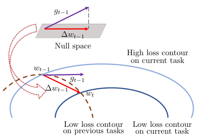
In this paper, we focus on the setting of continual learning where the datasets from previous tasks are inaccessible. We first propose two theoretical conditions respectively for stability and plasticity of deep networks in continual learning. Based on them, we design a novel network training algorithm called Adam-NSCL for continual learning, which forces the network parameter update to lie in the null space of the input features of previous tasks at each network layer, as shown in \figreffig:idea. The layer-wise null space of input features can be modeled as the null space of the uncentered covariance of these features, which can be incrementally computed after learning each task. Since it is too strict to guarantee the existence of null space, we approximate the null space of each layer by the subspace spanned by singular vectors corresponding to smallest singular values of the uncentered covariance of input features. We embed this strategy into the Adam optimization algorithm by projecting the candidate parameter update generated by Adam [21] into the approximate null space layer by layer, which is flexible and easy to implement.
We conduct various experiments on continual learning benchmarks in the setting that the datasets of previous tasks are unavailable, and results show that our Adam-NSCL is effective and outperforms the state-of-the-art continual learning methods. We also empirically verify the rationality of the approximate null space.
The paper is organized as follows. We first introduce related works in \secrefsec:related. In \secrefsec:method, we present the mathematical conditions and then propose network training algorithm for continual learning in \secrefsec:appro. In \secrefsec:exp, we conduct experiments to verify the efficacy of our approach.
2 Related Work
We next review the related works of continual learning in the following five categories.
Regularization-based strategy. The basic idea of this strategy is to penalize the changes of network parameters when learning current task to prevent catastrophic forgetting. The typical methods include EWC [22], SI [55], MAS [3], RWalk [6] and NPC [39]. They impose regularization on the network parameters, and each network parameter is associated with an importance weight computed by different methods. These importance weights are required to be stored for tasks in continual learning. Under the Bayesian framework, VCL [36], CLAW [2] and IMM [25] take the posterior distribution of network parameters learned from previous tasks as the prior distribution of network parameters on current task, which implicitly penalizes the changes of network parameters under the Bayesian framework.
Distillation-based strategy. Inspired by knowledge distillation [15], this strategy takes the network learned from previous tasks as teacher and the network being trained on current task as student, and then utilize a distillation term to alleviate performance degradation on previous tasks, such as LwF [27], GD-WILD [24], lifelong GAN [56], MCIL [30], LwM [10], etc. Due to inaccessibility to the full datasets of previous tasks, they commonly use data of current task [10, 27], external data [24], coreset of previous tasks [30, 44] or synthetic data [56], resulting in distributional shift [28] to the original datasets.
Replay-based strategy. The replay-based strategy trains networks using both data of the current task and “replayed” data of previous tasks. Some existing works focus on selecting a subset of data from previous tasks [4, 41], resulting in imbalance between the scale of datasets from current and previous tasks [51, 57]. An alternative approach is to learn generative model to generate synthetic data to substitute the original data [17, 20, 38, 47]. They do not need to store data of previous tasks, however, the performance is significantly affected by the quality of generated data, especially for complex natural images.
Architecture-based strategy. In this strategy, the network architecture is dynamically modified by expansion or mask operation when encountering new tasks in continual learning. Methods of network expansion modify the network architecture by increasing network width or depth to break its representational limit when facing new tasks [18, 26, 53]. This strategy may result in a powerful but redundant network that is computationally expensive and memory intensive. An alternative approach is to assign different sub-networks to different tasks by masking the neurons [1, 42, 46] or weights [32]. The mask associated with each task needs to be learned and stored in the memory.
Algorithm-based strategy. This strategy performs continual learning from the perspective of network training algorithm. It focuses on designing network parameter updating rule to guarantee that network training on current task should not deteriorate performance on previous tasks. GEM [31] computes the parameter update by solving a quadratic optimization problem constraining the angle between the parameter update and the gradients of network parameters on data of previous tasks. A-GEM [7] is an improved GEM without solving quadratic optimization problem. A-GEM constrains that the network parameter update should be well aligned with a reference gradient computed from a random batch of data from the previous tasks. Both of GEM and A-GEM need to store data of previous tasks. Different from GEM and A-GEM, OWM [54] projects the parameter update into the orthogonal space of the space spanned by input features of each linear layer. The computation of the space projection matrix relies on the unstable inversion of matrix.
Our method called Adam-NSCL is a novel network training algorithm for continual learning, which trains networks in the approximate null space of feature covariance matrix of previous tasks to balance the network plasticity and stability. It does not require to design regularizers, revise network architecture and use replayed data in our method. Compared with OWM, Adam-NSCL relies on null space of feature covariance for achieving plasticity and stability with theoretical and empirical analysis, and overcomes the unstable matrix inversion in OWM. More discussions on the differences are in \secrefexpres.
3 Analysis of Stability and Plasticity
In this section, we first present the preliminaries on the setting of continual learning, then propose mathematical conditions on the network parameter updates for the stability and plasticity, as the basis of our algorithm in \secrefsec:appro.
3.1 Preliminaries
In the setting of continual learning, a network with parameters is sequentially trained on a stream of tasks , where task is associated with paired dataset of size . The output of network on data is denoted as .
The initial parameters of network with linear layers on task is set as which is the optimal parameters after trained on task . When training on task at the -th training step, we denote the network parameters as . Correspondingly, the parameter update at the -th training step on task is denoted as . When feeding data from task to with optimal parameters on task , the input feature and output feature at the -th linear layer are denoted as and , then
with as the nonlinear function and .
For the convolutional layer, we can reformulate convolution as the above matrix multiplication, which is unified with the fully-connected layer. Specifically, for each 3-D feature map, we flat each patch as a row vector, where the patch size is same as the corresponding 3-D convolutional kernel size, and the number of patches is the times that the kernel slides on the feature map when convolution. Then these row-wise vectors are concatenated to construct the 2-D feature matrix . 3-D kernels at the same layer are flatted as column vectors of the 2-D parameter matrix.
3.2 Conditions for continual learning
When being trained on the current task without training data from previous tasks, the network is expected to perform well on the previous tasks, which is challenging since the network suffers from catastrophic forgetting. To alleviate the plasticity-stability dilemma, we propose two conditions for continual learning that guarantee the stability and plasticity respectively as follows.
To derive Condition 1 for network stability, we first present the condition of network parameter update to retain training performance on succeeding training tasks in Lemma 1 and Lemma 2, depending on data of previous tasks. Then, we further propose the equivalent condition in Condition 1, free from storing data of previous tasks. After that, we present Condition 2 for network plasticity.
Lemma 1.
Given the data from task , and the network with linear layers is trained on task (). If network parameter update lies in the null space of , \ie,
| (1) |
at each training step , for the -th layer of , we have and .
Proof.
Please refer to the supplemental material. ∎
Lemma 1 tells us that, when we train network on task , the network retains its training loss on data in the training process, if the network parameter update satisfies Eqn. (1) at each training step. Considering that we initialize parameters by , \ie, the optimal parameters on task for , we have the following corollary.
Corollary 1.
Assume that network is sequentially trained on tasks . For each task and , if Eqn. (1) holds at every training step on task , we have and .
Corollary 1 suggests that the training loss on data is retained if the network trained on the following tasks satisfies Eqn. (1) and network parameters at each task are initialized by the trained network of the last task.
We further denote , which is the concatenation of input features of -th network layer on each task data () using trained network parameters on task . Then the following lemma holds.
Lemma 2.
Assume that is being trained on task (). If lies in the null space of at each training step , \ie,
| (2) |
for , we have for all .
Lemma 2 guarantees the stability of . However, it is inefficient since it requires to store all features of for all , which is memory-prohibited. To overcome this limitation, we propose the following Condition 1 based on uncentered feature covariance to guarantee stability, where is the total number of seen data, \ie, the number of rows of .
Condition 1 (stability).
When is being trained on task , at each training step should lie in the null space of the uncentered feature covariance matrix for , \ie,
| (3) |
It is easy to verify that the null space of equals to null space of the uncentered feature covariance of . Therefore, if Condition 1 holds, we have for all according to Lemma 2, \ie, the performance of on previous task data will not be degraded after learning current task.
Memory analysis. The memory consumption of storing is fixed, irrelevant to the number of tasks and data. Specifically, if we denote the dimension of the feature at layer as , the size of is (usually ), while the size of is . Therefore, Condition 1 supplies a more memory efficient way to guarantee the stability of than Lemma 2.
Condition 1 guarantees the stability of network in continual learning. The other requirement of continual learning is the plasticity of concerning the ability to obtain new knowledge from current task. Condition 2 will provide the condition that guarantees the plasticity of network .
Condition 2 (plasticity).
Assume that the network is being trained on task , and denotes the parameter update generated by a gradient-descent training algorithm for training at training step . should hold where represents inner product.
If parameter update satisfies Condition 2 when training on task , the training loss after updating parameters using will decrease, \ie, the network can be trained on this task. Please see supp. for proof.
4 Network Training in Covariance Null Space
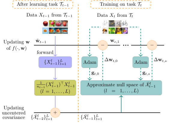
In this section, we propose a novel network training algorithm called Adam-NSCL for continual learning based on Adam and the proposed two conditions respectively for stability and plasticity. In continual learning, we maintain layer-wise feature covariance matrices, which are incrementally updated using features of the coming task. Given the current task, starting from the network trained on previous tasks, we update the network parameters on current task using Adam-NSCL where the candidate parameter update generated by Adam is projected into the approximate null space of corresponding feature covariance matrix layer by layer to balance the network stability and plasticity.
Figure 2 illustrates the pipeline of our proposed continual learning algorithm. After learning task , we feed to the learned network to get the input feature at each layer. Then we compute the uncentered covariance with as the number of data on task . Subsequently, we update the uncentered feature covariance matrix for each layer by
| (4) |
with as the total number of seen data. Following that, we compute the approximate null space of . When training network with as initialization on task , we first utilize Adam to generate a candidate parameter update at -th step (), then project into the approximate null space of layer by layer to get the parameter update .
In the following, we first introduce derivation of the approximate null space in \secrefsec:appns, and discuss the projection satisfying Conditions 1 and 2. Subsequently, we present our proposed continual learning algorithm in \AlgRefalg and the way to find the approximate null space in \AlgRefalg:null.
4.1 Approximate null space
According to Condition 1, for the stability of network in continual learning, we can force the parameter update to lie in the null space of uncentered covariance of all previous input features at each network layer. However, it is too strict to guarantee the existence of null space. Therefore, we propose \AlgRefalg:null to find the approximate null space based on SVD of the uncentered covariance matrix.
By applying SVD to , we have
| (5) |
where and . If all singular values of zero are in , \ie, , then holds, since is an unitary matrix. It suggests that the range space of is the null space of . Thus we can get the parameter update lying in the null space of by
| (6) |
with as projection operator [35, Eqn. (5.13.4)]. Thus we get satisfying Condition 1.
Inputs: Datasets for task ; network with linear layers; learning rate .
Initialization: Initialize randomly, , number of seen data .
However, it is unrealistic to guarantee that there exists zero singular values. Inspired by Principal Component Analysis, if considering as principal components, can be approximated by , which indicates that , \ie, we can take the range space of as the approximate null space of where corresponds to the smallest singular values in . We adaptively select with diagonal singular values , where is the smallest singular value. Furthermore, to empirically verify the rationality of the approximation, we utilize the proportion of explained by [19] as
| (7) |
where “diag” denotes the diagonal elements. If is small, the sum of singular values of is negligible, suggesting that it is reasonable to approximate null space of uncentered covariance matrix by the range space of .
Inputs: Dateset of size for task ; network ; ; hyperparameter ; number of seen data .
Output: ; ;
Example. We take the pretrained ResNet-18 on dataset of ImageNet ILSVRC 2012 [45] as example. Figure 3 shows the curves of singular values of uncentered covariance matrix of each linear layer indexed by with . All proportions of different layers are smaller than 0.05, indicating that the selected corresponding to smallest singular values is negligible to explain . Therefore, it is reasonable to approximate the null space by the range space of .
As a summary, for a novel task , our continual learning algorithm (shown in \figreffigalg) projects parameter update at -th training step generated by Adam into the approximate null space layer by layer, and get the parameter update following Eqn. (6). We prove that always holds, which can be found in the supplemental material. To guarantee that the network can be trained on task using the above parameter updating rule, it is supposed that as discussed in Condition 2. We empirically found that it holds in our experiments and our algorithm can succeed in decreasing training losses on sequential training tasks.
Our Adam-NSCL is summarized in \AlgRefalg. The training process is to loop over incoming tasks, and task () is trained by Adam with gradients projected into the null space of accumulated covariance (line 15 in \AlgRefalg). The null space is obtained by \AlgRefalg:null after learning task . In \AlgRefalg:null, we first feed all training data of task to accumulate covariance in lines 3-8, and update the uncentered covariance in line 10. Then we compute the approximate null space in lines 12-14 by SVD.
The hyperparameter controls the balance of stability and plasticity. Larger suggests that we use larger approximate null space covering more small singular values, then the null space assumption in Eqn. (3) hardly holds, reducing the stability in continual learning. On the other hand, larger leads to larger approximate null space, enabling us to update network parameters in a larger null space, increasing the plasticity to learn knowledge on current task.
5 Experiments
We apply Adam-NSCL algorithm to different sequential tasks for continual learning11 1 https://github.com/ShipengWang/Adam-NSCL. After introducing experimental setting, we show the results compared with SOTA methods, following which we empirically analyze our algorithm.
5.1 Experimental setting
We first describe the experimental settings on datasets, implementation details, metrics and compared methods.
Datasets. We evaluate on continual learning datasets, including 10-split-CIFAR-100, 20-split-CIFAR-100 and 25-split-TinyImageNet. 10-split-CIFAR-100 and 20-split-CIFAR-100 are constructed by splitting CIFAR-100 [23] into 10 and 20 tasks, and the classes in different tasks are disjoint. 25-split-TinyImageNet is constructed by splitting TinyImageNet [50] containing RGB images into 25 tasks, which is a harder setting due to longer sequence.
Implementation details. Adam-NSCL is implemented using PyTorch [40]. We take ResNet-18 [14] as the backbone network in our experiments. All tasks share the same backbone network but each task has its own classifier. The classifier will be fixed after the model is trained on the corresponding task. For batch normalization layer, we regularize its parameters using EWC [22]. The learning rate starts from and decays at epoch 30, 60 with a multiplier 0.5 (80 epochs in total). The batch size is set to 32 for 10-split-CIFAR-100 and 16 for the other two datasets. The regularizer coefficient of EWC for penalizing parameters at batch normalization is set to 100. At each linear layer, to approximate null space of uncentered covariance, we set for 20-split-CIFAR-100 while for the other two datasets. We also study the effect of in \secrefsec:ana.
Compared methods. We compare our method with various continual learning methods including EWC [22], MAS [3], MUC-MAS [29], SI [38], LwF [27], GD-WILD [24], GEM, [31], A-GEM [7], MEGA [13], InstAParam [8] and OWM [54]. For a fair comparison, the backbone networks employed in these methods are all ResNet-18. EWC, MAS, MUC-MAS and SI regularize the changes of parameters across tasks, where each parameter is associated with a weight of importance. LwF and GD-WILD are based on knowledge distillation using different dataset for distillation to preserve learned knowledge on previous tasks. GEM, A-GEM, MEGA and OWM focus on designing network training algorithm to overcome forgetting. InstAParam is based on architecture-based strategy. Among these methods, EWC, MAS, MUC-MAS and SI need to store the importance weight in memory, GD-WILD, GEM A-GEM and MEGA need to store data of previous tasks, and OWM needs to store the projection matrix which is incrementally computed with an approximate inversion of matrix.
Evaluation metrics. We employ the evaluation metrics proposed in [31], including backward transfer (BWT) and average accuracy (ACC). BWT is the average drop of accuracy of the network for test on previous tasks after learning current task. Negative value of BWT indicates the degree of forgetting in continual learning. ACC is the average accuracy of the network on test datasets of all seen tasks. With similar ACC, the one having larger BWT is better.
5.2 Experimental results
We next compare different continual learning algorithms. The details on the comparative results on three datasets are presented as follows.
| Method | 10-split-CIFAR-100 | |
|---|---|---|
| ACC (%) | BWT(%) | |
| EWC [22] | 70.77 | -2.83 |
| MAS [3] | 66.93 | -4.03 |
| MUC-MAS [29] | 63.73 | -3.38 |
| SI [38] | 60.57 | -5.17 |
| LwF [27] | 70.70 | -6.27 |
| InstAParam [8] | 47.84 | -11.92 |
| ∗GD-WILD [24] | 71.27 | -18.24 |
| ∗GEM [31] | 49.48 | 2.77 |
| ∗A-GEM [7] | 49.57 | -1.13 |
| ∗ MEGA [13] | 54.17 | -2.19 |
| OWM [54] | 68.89 | -1.88 |
| Adam-NSCL | 73.77 | -1.6 |
10-split-CIFAR-100. The comparative results on 10-split-CIFAR-100 are illustrated in \tabreffinal10, where the proposed Adam-NSCL achieves the highest ACC 73.77% with competitive BWT -1.6%. The BWT values of GEM and A-GEM are better than Adam-NSCL, however, their ACC values are 49.48% and 49.57%, significantly lower than ours. EWC, LwF and GD-WILD achieve marginally worse ACC compared with Adam-NSCL, but the BWT values of LwF and GD-WILD are much lower. Both ACC and BWT values of MAS, MUC-MAS and SI are much lower than ours. OWM has comparable BWT with our Adam-NSCL, but the ACC of OWM is 4.88% lower than ours. Overall, our Adam-NSCL is the most preferable method among all these compared methods for continual learning.
To justify the rationality of approximate null space, we show the curves of singular values in descending order and proportion values of defined in Eqn. (7) for the 2-th, 7-th, 12-th and 17-th layers of network in \figrefexp1eigen on sequential tasks. As the results indicate, all proportion values of are smaller than 0.05, indicating that it is reasonable to take the range space of insignificant components as the approximate null space at the -th layer .
| Method | 20-split-CIFAR-100 | |
|---|---|---|
| ACC (%) | BWT(%) | |
| EWC [22] | 71.66 | -3.72 |
| MAS [3] | 63.84 | -6.29 |
| MUC-MAS [29] | 67.22 | -5.72 |
| SI [38] | 59.76 | -8.62 |
| LwF [27] | 74.38 | -9.11 |
| InstAParam [8] | 51.04 | -4.92 |
| ∗GD-WILD [24] | 77.16 | -14.85 |
| ∗GEM [31] | 68.89 | -1.2 |
| ∗A-GEM [7] | 61.91 | -6.88 |
| ∗MEGA [13] | 64.98 | -5.13 |
| OWM [54] | 68.47 | -3.37 |
| Adam-NSCL | 75.95 | -3.66 |
20-split-CIFAR-100. The comparisons on 20-split-CIFAR-100 dataset are shown in \tabreffinal20. Our method achieves the second best ACC 75.95%. Though GD-WILD achieves 1.21% higher ACC than ours, the BWT of GD-WILD is 11.19% lower than that of our Adam-NSCL. Furthermore, GD-WILD requires to save data of previous tasks and a large mount of external data. EWC, GEM and OWM achieve 4.29%, 7.06% and 7.48% lower ACC values compared with our method. LwF has marginally lower ACC than ours, but its BWT value is significantly worse than ours. Other methods including MAS, MUC-MAS, SI and A-GEM fail to achieve comparable results as ours. Therefore, our Adam-NSCL outperforms the other compared methods for continual learning.
| Method | 25-split-TinyImageNet | |
|---|---|---|
| ACC (%) | BWT(%) | |
| EWC [22] | 52.33 | -6.17 |
| MAS [3] | 47.96 | -7.04 |
| MUC-MAS [29] | 41.18 | -4.03 |
| SI [38] | 45.27 | -4.45 |
| LwF [27] | 56.57 | -11.19 |
| InstAParam [8] | 34.64 | -10.05 |
| ∗GD-WILD [24] | 42.74 | -34.58 |
| ∗A-GEM [7] | 53.32 | -7.68 |
| ∗MEGA [13] | 57.12 | -5.90 |
| OWM [54] | 49.98 | -3.64 |
| Adam-NSCL | 58.28 | -6.05 |
25-split-TinyImageNet. As shown in \tabreffinaltiny, on 25-split-TinyImageNet dataset, the proposed Adam-NSCL outperforms the other compared methods with the best ACC and competitive BWT values. Specifically, Adam-NSCL achieves the best ACC 58.28% with comparable BWT -6.05%. Though the BWT of Adam-NSCL is marginally lower than MUC-MAS, SI and OWM, these compared methods achieve 16.68%, 13.01% and 8.3% lower ACC than ours. LwF achieves the second best ACC, but with much inferior BWT compared with our Adam-NSCL. With marginally lower BWT, EWC and MAS achieve 5.95% and 10.32% lower ACC than Adam-NSCL.
We now discuss the difference between Adam-NSCL and OWM [54]. The main difference of Adam-NSCL and OWM is the way to find the null space as discussed in \secrefsec:related. Computing the projection matrix in OWM relies on the approximate generalized inversion of feature matrix, and the approximate error can be accumulated when incrementally update the projection matrix. While in Adam-NSCL, the null space is specified by the uncentered feature covariance which can be incrementally computed without approximate error. Additionally, Adam-NSCL consistently performs better than OWM on 10-split-CIFAR-100 and 20-split-CIFAR-100, as shown in Tabs. 1 and 2, where Adam-NSCL achieves 4.88% and 7.48% larger ACC and similar BWT in comparison with OWM respectively. On 25-split-TinyImageNet, Adam-NSCL has significantly better ACC with comparable BWT than OWM, as shown in \tabreffinaltiny.
5.3 Model analysis
Stability and plasticity analysis. To study the balance of stability and plasticity, which is controlled by , we compare the performance of our Adam-NSCL by varying . According to \figrefex:balance, BWT becomes worse when is larger, suggesting that the network forgets more learned knowledge of previous tasks with lager . Since ACC is affected by both of stability and plasticity, it increases first and then decreases with the increase of at the middle and bottom sub-figures of \figrefex:balance.
Evolution of training loss. To justify the proposed Adam-NSCL indeed guarantees the stability of network training on sequential tasks, we show the curves of training losses on the tasks after learning new tasks in \figrefexp:loss on 10-split-CIFAR-100. According to \figrefexp:loss, the training losses of the network on previous tasks are retained after learning new tasks, verifying that Adam-NSCL, with Condition 1 as basis, guarantees the stability of network.
6 Conclusion
In this paper, we address the plasticity-stability dilemma for continual learning, constraining that the datasets of previous tasks are inaccessible. We propose two theoretical conditions to guarantee stability and plasticity for network parameter update when training networks on sequential tasks. Then we design a novel continual learning algorithm Adam-NSCL, which is based on Adam. The candidate parameter update generated by Adam is projected into the approximate null space of uncentered feature covariance matrix of previous tasks. Extensive experiments show that the proposed algorithm outperforms the compared methods for continual learning. In the future, we consider to further improve the approximation of null space and conduct theoretical analysis for our algorithm.
Acknowledgment. This work was supported by NSFC (U20B2075, 11690011, 11971373, U1811461, 12026605) and National Key R&D Program 2018AAA0102201.
Supplemental Materials
We first introduce additional notations here. When feeding data from task to with parameters , the input feature and output feature at the -th linear layer are denoted as and respectively, then
with . In addition, by denoting the learning rate as , we have
Appendix A
In this appendix, we show the proof of Lemma 1 in the manuscript. Lemma 1 tells us that, when we train network on task , the network retains its training loss on data in the training process, if the network parameter update satisfies Eqn. (8) at each training step. We first recall Lemma 1 as follows, then give the proof.
Lemma 1.
Given the data from task , and the network with linear layers is trained on task (). If network parameter update lies in the null space of , \ie,
| (8) |
at each training step , for the -th layer of , we have and .
Proof.
The proof is based on the recursive structure of network and iterative training process. We first prove that and hold for , and then illustrate that and hold for each , which suggests that Lemma 1 holds.
When , considering that we initialize parameters , we have
| (9) |
Therefore, at the first layer where (all of them equal to when ),
| (10) |
where the fourth equation holds due to Eqn. (8). Furthermore, we have
| (11) |
, the input feature equals to at the second linear layer, based on which, we can recursively prove that
and
for by replacing with in Eqns. (Proof.) and (11), then we have .
We now have proved that , and hold for . Considering the iterative training process, we can prove that
and
hold for , by repeating the above process with .
Finally, we have and , since Lemma 1 holds for each . ∎
Appendix B
We first recall the Condition 2 in the manuscript as follows, then prove that parameter update satisfying condition 2 is the descent direction, \ie, the training loss after updating parameters using will decrease.
Condition 2 (plasticity).
Assume that the network is being trained on task , and denotes the parameter update generated by a gradient-descent training algorithm for training at training step . should hold where represents inner product.
We now discuss the reason why is the descent direction, if it satisfies condition 2. For clarity, we denote the loss for training network as which ignores the data term with no effect. The discussion can also be found in Lemma 2 of the lecture22 2 http://www.princeton.edu/~aaa/Public/Teaching/ORF363_COS323/F14/ORF363_COS323_F14_Lec8.pdf.
By denoting the learning rate as , and , according to Taylor’s theorem, we have
,
where when . Therefore, there exists such that
Together with the condition , we can conclude that for all . Therefore, parameter update satisfying condition 2 is the descent direction.
Appendix C
Here, we give the proof of with , which is claimed in Sec 4.1 of the manuscript. The proof mainly utilizes the properties of Kronecker product [12, Eqns. (2.10) and (2.13)].
| (12) |
where vec is the vectorization of , is the identity matrix and is the Kronecker product.
Appendix D
We now discuss the difference between our algorithm and OWM [54] in details as follows. (1) We provide novel theoretical conditions for the stability and plasticity of network based on feature covariance. (2) The null space of ours is defined as the null space of feature covariance matrix which is easy to be accumulated after each task (refer to Q1 & Alg. 2). While the projection matrix in OWM is where consists of all previous features of layer . (3) With the coming of new tasks, our covariance matrix is incrementally updated without approximation error, while of OWM is updated by recursive least square, where the approximation error of matrix inversion (because of the additionally introduced ) will be accumulated. (4) Our approach relies on a hyperparameter in line 14 of Alg. 2, for approximating the null space of covariance, which can balance the stability and plasticity as discussed in lines 572-579 and Fig. 5. It is easy to set the hyperparameter (line 614 and Figs. 4, 5). But we find that it is hard to tune the hyperparameter in OWM for each layer to balance the approximation error and computational stability. (5) Experimental comparison with OWM on three benchmarks are shown in Tabs. 1-3. The ACC of ours are 4.88%, 7.48% and 8.3% higher than OWM with comparable BWT. Please refer to Q4 for comparison on ImageNet with deeper networks. We will clarify these differences by extending the discussions in Sect. 2.
References
- [1] Davide Abati, Jakub Tomczak, Tijmen Blankevoort, Simone Calderara, Rita Cucchiara, and Babak Ehteshami Bejnordi. Conditional channel gated networks for task-aware continual learning. In IEEE Conf. Comput. Vis. Pattern Recog., pages 3931–3940, 2020.
- [2] Tameem Adel, Han Zhao, and Richard E Turner. Continual learning with adaptive weights (claw). In Int. Conf. Learn. Represent., 2019.
- [3] Rahaf Aljundi, Francesca Babiloni, Mohamed Elhoseiny, Marcus Rohrbach, and Tinne Tuytelaars. Memory aware synapses: Learning what (not) to forget. In Eur. Conf. Comput. Vis., pages 139–154, 2018.
- [4] Rahaf Aljundi, Min Lin, Baptiste Goujaud, and Yoshua Bengio. Gradient based sample selection for online continual learning. In Adv. Neural Inform. Process. Syst., pages 11816–11825, 2019.
- [5] Dzmitry Bahdanau, Kyunghyun Cho, and Yoshua Bengio. Neural machine translation by jointly learning to align and translate. In Int. Conf. Learn. Represent., 2015.
- [6] Arslan Chaudhry, Puneet K Dokania, Thalaiyasingam Ajanthan, and Philip HS Torr. Riemannian walk for incremental learning: Understanding forgetting and intransigence. In Eur. Conf. Comput. Vis., pages 532–547, 2018.
- [7] Arslan Chaudhry, Marc’Aurelio Ranzato, Marcus Rohrbach, and Mohamed Elhoseiny. Efficient lifelong learning with a-gem. In Int. Conf. Learn. Represent., 2018.
- [8] Hung-Jen Chen, An-Chieh Cheng, Da-Cheng Juan, Wei Wei, and Min Sun. Mitigating forgetting in online continual learning via instance-aware parameterization. In Adv. Neural Inform. Process. Syst., 2020.
- [9] Jacob Devlin, Ming-Wei Chang, Kenton Lee, and Kristina Toutanova. Bert: Pre-training of deep bidirectional transformers for language understanding. arXiv preprint arXiv:1810.04805, 2018.
- [10] Prithviraj Dhar, Rajat Vikram Singh, Kuan-Chuan Peng, Ziyan Wu, and Rama Chellappa. Learning without memorizing. In IEEE Conf. Comput. Vis. Pattern Recog., pages 5138–5146, 2019.
- [11] Robert M French. Catastrophic forgetting in connectionist networks. Trends Cogn. Sci., 3(4):128–135, 1999.
- [12] Alexander Graham. Kronecker products and matrix calculus with applications. Courier Dover Publications, 2018.
- [13] Yunhui Guo, Mingrui Liu, Tianbao Yang, and Tajana Rosing. Improved schemes for episodic memory-based lifelong learning. In Adv. Neural Inform. Process. Syst., 2020.
- [14] Kaiming He, Xiangyu Zhang, Shaoqing Ren, and Jian Sun. Identity mappings in deep residual networks. In Eur. Conf. Comput. Vis., pages 630–645, 2016.
- [15] Geoffrey Hinton, Oriol Vinyals, and Jeff Dean. Distilling the knowledge in a neural network. In Adv. Neural Inform. Process. Syst. Worksh., 2015.
- [16] Yen-Chang Hsu, Yen-Cheng Liu, Anita Ramasamy, and Zsolt Kira. Re-evaluating continual learning scenarios: A categorization and case for strong baselines. In Adv. Neural Inform. Process. Syst. Worksh., 2018.
- [17] Wenpeng Hu, Zhou Lin, Bing Liu, Chongyang Tao, Zhengwei Tao, Jinwen Ma, Dongyan Zhao, and Rui Yan. Overcoming catastrophic forgetting for continual learning via model adaptation. In Int. Conf. Learn. Represent., 2018.
- [18] Ching-Yi Hung, Cheng-Hao Tu, Cheng-En Wu, Chien-Hung Chen, Yi-Ming Chan, and Chu-Song Chen. Compacting, picking and growing for unforgetting continual learning. In Adv. Neural Inform. Process. Syst., pages 13669–13679, 2019.
- [19] Ian T Jolliffe and Jorge Cadima. Principal component analysis: a review and recent developments. Philos. Trans. R. Soc. A, 374(2065), 2016.
- [20] Ronald Kemker and Christopher Kanan. Fearnet: Brain-inspired model for incremental learning. In Int. Conf. Learn. Represent., 2018.
- [21] Diederik P Kingma and Jimmy Ba. Adam: A method for stochastic optimization. In Int. Conf. Learn. Represent., 2015.
- [22] James Kirkpatrick, Razvan Pascanu, Neil Rabinowitz, Joel Veness, Guillaume Desjardins, Andrei A Rusu, Kieran Milan, John Quan, Tiago Ramalho, Agnieszka Grabska-Barwinska, et al. Overcoming catastrophic forgetting in neural networks. Proc. Natl. Acad. Sci. USA, 114(13):3521–3526, 2017.
- [23] Alex Krizhevsky et al. Learning multiple layers of features from tiny images. Technical report, University of Toronto, 2009.
- [24] Kibok Lee, Kimin Lee, Jinwoo Shin, and Honglak Lee. Overcoming catastrophic forgetting with unlabeled data in the wild. In Int. Conf. Comput. Vis., pages 312–321, 2019.
- [25] Sang-Woo Lee, Jin-Hwa Kim, Jaehyun Jun, Jung-Woo Ha, and Byoung-Tak Zhang. Overcoming catastrophic forgetting by incremental moment matching. In Adv. Neural Inform. Process. Syst., pages 4652–4662, 2017.
- [26] Xilai Li, Yingbo Zhou, Tianfu Wu, Richard Socher, and Caiming Xiong. Learn to grow: A continual structure learning framework for overcoming catastrophic forgetting. In Int. Conf. Mach. Learn., pages 3925–3934, 2019.
- [27] Zhizhong Li and Derek Hoiem. Learning without forgetting. IEEE Trans. Pattern Anal. Mach. Intell., 40(12):2935–2947, 2017.
- [28] Xialei Liu, Chenshen Wu, Mikel Menta, Luis Herranz, Bogdan Raducanu, Andrew D. Bagdanov, Shangling Jui, and Van De Weijer Joost. Generative feature replay for class-incremental learning. In IEEE Conf. Comput. Vis. Pattern Recog. Worksh., 2020.
- [29] Yu Liu, Sarah Parisot, Gregory Slabaugh, Xu Jia, Ales Leonardis, and Tinne Tuytelaars. More classifiers, less forgetting: A generic multi-classifier paradigm for incremental learning. In Eur. Conf. Comput. Vis., 2020.
- [30] Yaoyao Liu, Yuting Su, An-An Liu, Bernt Schiele, and Qianru Sun. Mnemonics training: Multi-class incremental learning without forgetting. In IEEE Conf. Comput. Vis. Pattern Recog., pages 12245–12254, 2020.
- [31] David Lopez-Paz and Marc’Aurelio Ranzato. Gradient episodic memory for continual learning. In Adv. Neural Inform. Process. Syst., pages 6467–6476, 2017.
- [32] Arun Mallya, Dillon Davis, and Svetlana Lazebnik. Piggyback: Adapting a single network to multiple tasks by learning to mask weights. In Eur. Conf. Comput. Vis., pages 67–82, 2018.
- [33] Michael McCloskey and Neal J Cohen. Catastrophic interference in connectionist networks: The sequential learning problem. In Psychol. Learn. Motiv. Elsevier, 1989.
- [34] Martial Mermillod, Aurélia Bugaiska, and Patrick Bonin. The stability-plasticity dilemma: Investigating the continuum from catastrophic forgetting to age-limited learning effects. Front. Psychol., 4:504, 2013.
- [35] Carl D Meyer. Matrix analysis and applied linear algebra, volume 71. Siam, 2000.
- [36] Cuong V Nguyen, Yingzhen Li, Thang D Bui, and Richard E Turner. Variational continual learning. In Int. Conf. Learn. Represent., 2018.
- [37] Oleksiy Ostapenko, Mihai Puscas, Tassilo Klein, Patrick Jahnichen, and Moin Nabi. Learning to remember: A synaptic plasticity driven framework for continual learning. In IEEE Conf. Comput. Vis. Pattern Recog., pages 11321–11329, 2019.
- [38] Oleksiy Ostapenko, Mihai Puscas, Tassilo Klein, Patrick Jahnichen, and Moin Nabi. Learning to remember: A synaptic plasticity driven framework for continual learning. In IEEE Conf. Comput. Vis. Pattern Recog., pages 11321–11329, 2019.
- [39] Inyoung Paik, Sangjun Oh, Tae-Yeong Kwak, and Injung Kim. Overcoming catastrophic forgetting by neuron-level plasticity control. In AAAI, pages 5339–5346, 2020.
- [40] Adam Paszke, Sam Gross, Francisco Massa, Adam Lerer, James Bradbury, Gregory Chanan, Trevor Killeen, Zeming Lin, Natalia Gimelshein, Luca Antiga, Alban Desmaison, Andreas Kopf, Edward Yang, Zachary DeVito, Martin Raison, Alykhan Tejani, Sasank Chilamkurthy, Benoit Steiner, Lu Fang, Junjie Bai, and Soumith Chintala. Pytorch: An imperative style, high-performance deep learning library. In Adv. Neural Inform. Process. Syst., pages 8024–8035, 2019.
- [41] Ameya Prabhu, Philip HS Torr, and Puneet K Dokania. Gdumb: A simple approach that questions our progress in continual learning. In Eur. Conf. Comput. Vis., 2020.
- [42] Jathushan Rajasegaran, Munawar Hayat, Salman H Khan, Fahad Shahbaz Khan, and Ling Shao. Random path selection for continual learning. In Adv. Neural Inform. Process. Syst., pages 12669–12679, 2019.
- [43] Roger Ratcliff. Connectionist models of recognition memory: constraints imposed by learning and forgetting functions. Psychol. Rev., 97(2):285, 1990.
- [44] Sylvestre-Alvise Rebuffi, Alexander Kolesnikov, Georg Sperl, and Christoph H Lampert. icarl: Incremental classifier and representation learning. In IEEE Conf. Comput. Vis. Pattern Recog., pages 2001–2010, 2017.
- [45] Olga Russakovsky, Jia Deng, Hao Su, Jonathan Krause, Sanjeev Satheesh, Sean Ma, Zhiheng Huang, Andrej Karpathy, Aditya Khosla, Michael Bernstein, Alexander C. Berg, and Li Fei-Fei. ImageNet Large Scale Visual Recognition Challenge. Int. J. Comput. Vis., 115(3):211–252, 2015.
- [46] Joan Serra, Didac Suris, Marius Miron, and Alexandros Karatzoglou. Overcoming catastrophic forgetting with hard attention to the task. In Int. Conf. Mach. Learn., pages 4548–4557, 2018.
- [47] Hanul Shin, Jung Kwon Lee, Jaehong Kim, and Jiwon Kim. Continual learning with deep generative replay. In Adv. Neural Inform. Process. Syst., pages 2990–2999, 2017.
- [48] David Silver, Aja Huang, Chris J Maddison, Arthur Guez, Laurent Sifre, George Van Den Driessche, Julian Schrittwieser, Ioannis Antonoglou, Veda Panneershelvam, Marc Lanctot, et al. Mastering the game of go with deep neural networks and tree search. nature, 529(7587):484–489, 2016.
- [49] Concetto Spampinato, Simone Palazzo, Isaak Kavasidis, Daniela Giordano, Nasim Souly, and Mubarak Shah. Deep learning human mind for automated visual classification. In IEEE Conf. Comput. Vis. Pattern Recog., pages 6809–6817, 2017.
- [50] Jiayu Wu, Qixiang Zhang, and Guoxi Xu. Tiny imagenet challenge. Technical report, Stanford University, 2017.
- [51] Yue Wu, Yinpeng Chen, Lijuan Wang, Yuancheng Ye, Zicheng Liu, Yandong Guo, and Yun Fu. Large scale incremental learning. In IEEE Conf. Comput. Vis. Pattern Recog., pages 374–382, 2019.
- [52] Yang Yan, Jian Sun, Huibin Li, and Zongben Xu. Deep admm-net for compressive sensing mri. In Adv. Neural Inform. Process. Syst., pages 10–18, 2016.
- [53] Jaehong Yoon, Eunho Yang, Jeongtae Lee, and Sung Ju Hwang. Lifelong learning with dynamically expandable networks. In Int. Conf. Learn. Represent., 2018.
- [54] Guanxiong Zeng, Yang Chen, Bo Cui, and Shan Yu. Continual learning of context-dependent processing in neural networks. Nat. Mach. Intell., 1(8):364–372, 2019.
- [55] Friedemann Zenke, Ben Poole, and Surya Ganguli. Continual learning through synaptic intelligence. In Int. Conf. Mach. Learn., pages 3987–3995, 2017.
- [56] Mengyao Zhai, Lei Chen, Frederick Tung, Jiawei He, Megha Nawhal, and Greg Mori. Lifelong gan: Continual learning for conditional image generation. In Int. Conf. Comput. Vis., pages 2759–2768, 2019.
- [57] Bowen Zhao, Xi Xiao, Guojun Gan, Bin Zhang, and Shu-Tao Xia. Maintaining discrimination and fairness in class incremental learning. In IEEE Conf. Comput. Vis. Pattern Recog., pages 13208–13217, 2020.