Discovering Diverse Solutions in Deep Reinforcement Learning by Maximizing State-Action-Based Mutual Information

Reinforcement learning (RL) has achieved significant success in various fields, including robotic manipulation [1, 2], board games [3], and optimization of experimental setups [4]. In RL, multiple optimal policies may exist that elicit the optimal value function [5]. For example, when learning a walking behavior at a certain speed, there are often an infinite number of walking styles to achieve the specified speed. However, many existing RL methods are typically limited to obtaining only one of the optimal policies in a stochastic manner.

Recent studies investigated methods for learning diverse solutions and demonstrated their benefits. For instance, [6] demonstrated that unseen tasks can be solved rapidly by adapting diverse solutions of seen tasks, and [7] showed that learned diverse skills can be used as low-level policies of hierarchical RL for the performance improvement. Existing methods for learning diverse behaviors often maximize the mutual information (MI) by treating MI as unsupervised rewards [7, 6]. However, when treating MI as unsupervised rewards, we face the problem of function approximation which significantly affects the performance of actor-critic methods [8]. To stabilize the process for learning diverse solutions, it is desirable to develop a strategy for maximizing MI in a more stable manner.

The key contribution of our work is the proposal of a practical algorithm, latent-conditioned TD3 (LTD3), which can train a policy conditioned on a continuous or discrete latent variable and learn an infinite number of solutions. In our method, a policy conditioned on a latent variable is trained by directly maximizing a variational lower bound of MI, instead of treating MI as unsupervised rewards as in the previous studies [7, 6, 9]. Our method enables us to avoid the bias of the gradient estimator induced by value function approximation and steadily maximize MI. In addition, we also utilize a truncated importance sampling scheme for maximizing MI in a sample-efficient manner. Moreover, our method can be regarded as an approach that leverages separate critics for extrinsic and intrinsic rewards with different discount factors as in [10, 11]. We empirically investigated different strategies for maximizing MI and show that the our approach is sample-efficient and stable. While previous studies [7, 6, 12] often focused on learning a finite number of solutions, our experimental results demonstrate that our method can successfully learn a continuous skill space that encodes infinitely diverse behaviors, which is more challenging. $\Phi$ The effectiveness of our method in terms of few-shot robustness [6] was experimentally evaluated as shown in Figure 1, and our method outperformed baseline methods.

In this section, we describe definitions of terms related to an RL problem. Subsequently, we introduce the latent-conditioned policies for learning multiple solutions and describe the definition of few-shot robustness.

In this section, we formulate the problem of learning diverse solutions in RL. Subsequently, we describe our method to maximize the MI based on a variational lower bound.

In this section, we present a practical algorithm for learning a latent-conditioned policy based on TD3 [8], which is an actor-critic algorithm that learns a parameterized policy and parameterized Q-function. To approximate $Q^{\pi}({\boldsymbol{s}},{\boldsymbol{a}},{\boldsymbol{z}})$, we employ a differentiable function approximator $Q_{{\boldsymbol{w}}}$ parameterized by a vector ${\boldsymbol{w}}$, which is hereinafter referred to as the critic network.

We consider a deterministic policy as in deep deterministic policy gradient (DDPG) [22] and TD3 [8]. Therefore, $\pi({\boldsymbol{a}}|{\boldsymbol{s}},{\boldsymbol{z}})$ is a Dirac-delta function that satisfies

where ${\boldsymbol{\mu}}_{{\boldsymbol{\theta}}}({\boldsymbol{s}},{\boldsymbol{z}}):\mathcal{S}\times\mathcal{Z}\mapsto\mathcal{A}$ is a model parameterized by a vector ${\boldsymbol{\theta}}$ that determines action ${\boldsymbol{a}}$ for a specified state ${\boldsymbol{s}}$ in a deterministic manner. As in TD3, we employ two critic networks to stabilize the training, and they are trained by minimizing the mean squared error,

for $i=1,2$. Given $({\boldsymbol{s}},{\boldsymbol{a}},{\boldsymbol{s}}^{\prime},{\boldsymbol{z}},r)$, the target Q-value $y$ is computed as

and ${\boldsymbol{\sigma}}$ is the exploration noise variance. Herein, we use the same value of ${\boldsymbol{z}}$ as ${\boldsymbol{z}}$ to compute the next action ${\boldsymbol{a}}^{\prime}$. Therefore, the resulting $Q_{{\boldsymbol{w}}_{i}}({\boldsymbol{s}},{\boldsymbol{a}},{\boldsymbol{z}})$ approximates the expected return when following $\pi$ with the value of ${\boldsymbol{z}}$ fixed during an episode. The policy $\pi({\boldsymbol{a}}|{\boldsymbol{s}},{\boldsymbol{z}})$ is trained by maximizing

where $\mathcal{J}_{Q}({\boldsymbol{\theta}})$ is the term for maximizing the expected return based on the estimated Q-function, expressed as

The term $\mathcal{J}_{\textrm{info}}({\boldsymbol{\theta}},{\boldsymbol{\phi}})$ is expressed as

Herein, we refer to our TD3-based algorithm as Latent-conditioned TD3 (LTD3).

The proposed algorithm is summarized in Algorithm 1. The network architecture used in the LTD3 implementation is shown in Figure 2. In the network that models the latent-conditioned policy, the latent variable is input to a fully connected layer and then concatenated with the state vector. In the implementation, the conditional density $q_{{\boldsymbol{\phi}}}({\boldsymbol{z}}|{\boldsymbol{s}},{\boldsymbol{a}})$ is modeled by a neural network. We assume that the latent variable ${\boldsymbol{z}}$ is given by ${\boldsymbol{z}}=[{\boldsymbol{z}}_{\textrm{cont}},{\boldsymbol{z}}_{\textrm{disc}}]$ where ${\boldsymbol{z}}_{\textrm{cont}}$ and ${\boldsymbol{z}}_{\textrm{disc}}$ are continuous and discrete variables, respectively. We model $p({\boldsymbol{z}}_{\textrm{cont}}|{\boldsymbol{s}},{\boldsymbol{a}})$ as a factored Gaussian. For the categorical latent variable ${\boldsymbol{z}}_{\textrm{disc}}$, the categorical distribution $q_{{\boldsymbol{\phi}}}({\boldsymbol{z}}_{\textrm{disc}}|{\boldsymbol{s}},{\boldsymbol{a}})$ is modeled with a softmax layer. Whereas existing methods [6, 9] regard the MI term as unsupervised rewards, we directly maximize the information term via back-propagation in our method. In our framework, the gradient of the information term is back-propagated from the posteritor approximator to the policy network.

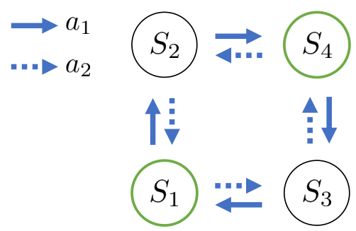
In existing studies, the MI between the state and latent variable $I({\boldsymbol{s}};{\boldsymbol{z}})$ was typically maximized [7, 6], which encourages different skills to visit different states. This strategy can encourage diversity in behaviors; however, maximizing state-only mutual information $I({\boldsymbol{s}};{\boldsymbol{z}})$ may not be sufficient to encourage diversity of behaviors. In Figure 3, we showcase an MDP where maximizing $I({\boldsymbol{s}},{\boldsymbol{a}};{\boldsymbol{z}})$ can encourage more diversity than maximizing $I({\boldsymbol{s}};{\boldsymbol{z}})$. As shown in Figure 3(a), two actions, $a_{1}$ and $a_{2}$ are allowed in each state in the MDP, and reward $r=1$ is given when state $S_{1}$ or $S_{4}$ are visited. different optimal policies for this MDP are shown in Figures 3(b) and (c). In practice, $I({\boldsymbol{s}};{\boldsymbol{z}})$ is maximized by estimating the posterior distribution $q({\boldsymbol{z}}|{\boldsymbol{s}})$, which predicts the value of the latent variable for a given state. However, as all states are equally visited by $\pi_{1}$ and $\pi_{2}$, $q({\boldsymbol{z}}|{\boldsymbol{s}})$ cannot quantify the difference between $\pi_{1}$ and $\pi_{2}$. Thus, maximizing $I({\boldsymbol{s}};{\boldsymbol{z}})$ cannot encourage the diversity of policies such as $\pi_{1}$ and $\pi_{2}$.

In contrast, we maximize $I({\boldsymbol{s}},{\boldsymbol{a}};{\boldsymbol{z}})$ to encode the diversity of both states and actions into the latent variable. The action-state mutual information $I({\boldsymbol{s}},{\boldsymbol{a}};{\boldsymbol{z}})$ is maximized by estimating the posterior distribution $q({\boldsymbol{z}}|{\boldsymbol{s}},{\boldsymbol{a}})$, not $q({\boldsymbol{z}}|{\boldsymbol{s}})$. Unlike $q({\boldsymbol{z}}|{\boldsymbol{s}})$, the posterior distribution $q({\boldsymbol{z}}|{\boldsymbol{s}},{\boldsymbol{a}})$ can quantify the difference between $\pi_{1}$ and $\pi_{2}$ by considering the corresponding action. Thus, maximizing $I({\boldsymbol{s}},{\boldsymbol{a}};{\boldsymbol{z}})$ can encourage diversity in policies such as $\pi_{1}$ and $\pi_{2}$. This example indicates that there are situations where maximizing $I({\boldsymbol{s}};{\boldsymbol{z}})$ is not sufficient and maximizing $I({\boldsymbol{s}},{\boldsymbol{a}};{\boldsymbol{z}})$ is more suitable.

Although we discussed the benefit of maximizing $I({\boldsymbol{s}},{\boldsymbol{a}};{\boldsymbol{z}})$, there are tasks where maximizing $I({\boldsymbol{s}};{\boldsymbol{z}})$ is sufficient. For example, previous studies have demonstrated that an agent can learn to walk in diverse directions by maximizing $I({\boldsymbol{s}};{\boldsymbol{z}})$. When training an agent to walk in diverse directions, the most important information is the agent destination, which is included in state ${\boldsymbol{s}}$. In such cases, maximizing $I({\boldsymbol{s}};{\boldsymbol{z}})$ can be sufficient because action ${\boldsymbol{a}}$ is not necessary to encourage the diversity of the walking directions.

In previous studies [6, 9], Soft Actor Critic (SAC)[23] was used as a base RL algorithm. Although SAC is a state-of-the-art actor critic method as well as TD3, we did not use SAC as a main base algorithm; instead, we used the TD3-based implementation in our study because of the following reason. If we use SAC as a base algorithm in our framework, $H({\boldsymbol{a}}|{\boldsymbol{s}},{\boldsymbol{z}})$ will be maximized because of the entropy regularization in SAC. In our framework, we maximize MI $I({\boldsymbol{s}},{\boldsymbol{a}};{\boldsymbol{z}})=H({\boldsymbol{s}},{\boldsymbol{a}})-H({\boldsymbol{a}}|{\boldsymbol{s}},{\boldsymbol{z}})-H({\boldsymbol{s}}|{\boldsymbol{z}})$. Therefore, maximization of $H({\boldsymbol{a}}|{\boldsymbol{s}},{\boldsymbol{z}})$ can conflict with that of $I({\boldsymbol{s}},{\boldsymbol{a}};{\boldsymbol{z}})$. In this sense, it is reasonable to use a deterministic policy for $\pi({\boldsymbol{a}}|{\boldsymbol{s}},{\boldsymbol{z}})$, which can be viewed as the limit of the normal distribution $\mathcal{N}(\mu,\sigma)$ as $\sigma\rightarrow 0$, resulting in $H({\boldsymbol{a}}|{\boldsymbol{s}},{\boldsymbol{z}})\rightarrow-\infty$. Therefore, we used TD3 as a based RL method.

Learning from expert demonstrations is effective for obtaining complex and natural motions [24]. In terms of imitation learning, the problem of imitating diverse behaviors from expert demonstrations has been addressed in previous studies [25, 26, 27, 28]. In these methods, diverse behaviors are encoded in latent variables. However, these imitation learning methods assume the availability of observations of diverse behaviors performed by experts. In this study, instead of learning from demonstrations, we address the problem of encoding diverse behaviors by learning from a reward function through trial and error.

In the field of evolutionary computation, QD algorithms that identify diverse solutions have been investigated [29, 30, 12, 31]. In these methods, multiple policies are trained to maximize both task-specific rewards and a behavior diversity metric. For example, [31] demonstrated that multiple solutions can be found for robotic manipulation tasks using a QD algorithm. However, these QD algorithms are typically limited to yielding a finite number of solutions. Our method can yield an infinite number of solutions by learning a continuous latent representation, thereby providing higher flexibility. Learning such continuous latent representations allows us to continuously tune the behavior of the agent through low-dimensional representations. Continuous control tasks often requires continuous tuning of the behavior of the agent, and continuous latent representations of diverse skills will be useful for downstream tasks.

Recently methods for learning diverse behaviors using deep RL with unsupervised rewards have been investigated [7, 9]. These methods can be used to learn a continuous skill space by training a latent-conditioned policy. However, these methods are not aimed at learning a policy to solve a specific task, and they learn diverse behaviors randomly. [6] proposed a method Structured Maximum Entropy Reinforcement Learning (SMERL), which learns multiple solutions for a specified task. However, information regarding the optimal return value before learning diverse solutions is required by that method. Therefore, a separate RL algorithm must be executed in advance to estimate the optimal return value because the optimal return value is typically unknown. By contrast, our method does not require information regarding the optimal return value, and a separate RL algorithm need not be executed. In other studies [10, 11, 32], the use of separate critics and different discount factors for extrinsic and intrinsic rewards in Atari games with discrete actions was investigated. Our method can be regarded as an approach that leverages separate critics for extrinsic and intrinsic rewards with different discount factors. Additionally, our method is applicable to problem domains with discrete actions by parameterizing $q({\boldsymbol{z}}|{\boldsymbol{s}},{\boldsymbol{a}})$ without an actor network.

Hierarchical RL methods [33, 34, 35, 36, 37] learn a hierarchical policy structured by a latent variable. However, the latent variable in HRL algorithms do not provide multiple solutions for a specified task. Recently, [35, 36] investigated goal-conditioned policies $\pi({\boldsymbol{a}}|{\boldsymbol{s}},{\boldsymbol{g}})$, where ${\boldsymbol{g}}$ denotes the goal. The goal-conditioned policy can be regarded as a method of modeling diverse behaviors conditioned on a latent variable that has semantic meaning. However, learning a goal-conditioned policy requires the user to specify the goals in a supervised manner. By contrast, we aim to learn diverse behaviors in an unsupervised manner by using only reward signals.

We performed experiments to evaluate 1) the diversity of solutions obtained by LTD3, 2) effect of strategies for maximizing MI, and 3) the few-shot robustness of policies obtained by LTD3. We used tasks based on OpenAI Gym [38] with MuJoCo physics engine [39]. The tasks were based on the Hopper, Walker2d, Humanoid, HalfCheetah, and Ant tasks, as shown in Figure 4¹¹ 1 Background color is changed from default setting for visibility.

To emphasize the existence of diverse solution, a velocity term of the reward function is modified from that in the original tasks in OpenAI Gym. In the reward function of the original tasks in OpenAI Gym, a velocity term $r_{\textrm{vel}}$ is used to encourage the agent to walk faster, and $r_{\textrm{vel}}$ is given by

where $x_{t}$ represents the horizontal position of the agent at time $t$, and $\Delta t$ is the time step size in the simulation. As in the study in [6], we modified the velocity term to the following:

where $v_{\textrm{max}}$ is a constant term that defines the upper bound of $r_{\textrm{vel}}$. Therefore, the agent is required to walk at the maximum speed $v_{\textrm{max}}$ with minimal control cost instead of walking as fast as possible. We refer to the modified version of the Hopper, Walker2d and Humanoid tasks as HopperVel, Walker2dVel, and HumanoidVel tasks, respectively. More details of these tasks are described in C.

We compared the proposed method with SMERL [6] and a variant of DIAYN [7], which is denoted as SAC-DIAYN herein and is used as a baseline in the study in [6]. In SAC-DIAYN, the policy is trained to maximize the sum of the task reward and an unsupervised reward given by $r_{\textrm{diayn}}=\log q_{{\boldsymbol{\psi}}}({\boldsymbol{z}}|{\boldsymbol{s}})$, where $q_{{\boldsymbol{\psi}}}({\boldsymbol{z}}|{\boldsymbol{s}})$ is a parameterized model that discriminates the value of the latent variable. Although [6] reported results based on discrete latent variables, this unsupervised reward can be applied to the continuous latent variable if a factored Gaussian distribution is assumed, as in [9]. In SMERL, $r_{\textrm{diayn}}$ is assigned only when the agent achieves a return that is close to the optimal return. Therefore, an off-the-shelf RL method must be used to determine the optimal return before executing SMERL. Our implementation of TD3 and SAC was adapted from the implementation in OpenAI Spinning Up [40].

We employed the diversity metric proposed in [12] to quantify the diversity of the learned solutions. Given a set of policies $\{\pi_{i}\}^{M}_{i=1}$, the diversity metric is given by

where ${\boldsymbol{\phi}}(\pi)\in\mathbb{R}^{l}$ is the behavior embedding of policy $\pi$, and $K:\mathbb{R}^{l}\times\mathbb{R}^{l}\mapsto\mathbb{R}$ is a kernel function. We used the squared-exponential kernel function given by

where $h$ is the length scale, and $h>0$. In our evaluation, we used $h=1000$ for the Ant task, and $h=100$ for the other tasks. As described in [12], we used the behavior embedding given by

which can be estimated using the states visited by policy $\pi$. To evaluate the diversity of solutions obtained by learning the continuous latent variable, we sampled the value of ${\boldsymbol{z}}$ uniformly from $[-1,1]$.

Although we demonstrated the advantage of the proposed method experimentally, the tasks used in our experiments are related to “how to walk” rather than “where to walk,” in which one can expect that actions contain meaningful information to obtain diverse behaviors. As demonstrated in previous studies [7, 6, 9], when state ${\boldsymbol{s}}$ contains sufficient information to encourage necessary diversity, maximizing $I({\boldsymbol{s}};{\boldsymbol{z}})$ is suitable.

In many off-policy actor-critic methods such as TD3 and SAC, the gradient with respect to the policy parameter is computed to maximize $\mathbb{E}[Q_{\boldsymbol{w}}({\boldsymbol{s}},{\boldsymbol{f}}_{\boldsymbol{\theta}}({\boldsymbol{s}}))]$, where $Q_{\boldsymbol{w}}({\boldsymbol{s}},{\boldsymbol{a}})$ is an approximated Q-function and ${\boldsymbol{f}}_{\boldsymbol{\theta}}({\boldsymbol{s}})$ is a function that represents a policy and generates actions. If there is an approximation error, the estimated gradient is biased unless the compatible function approximation is used [41, 42]. Furthermore, the error of the function approximation significantly affects the learning performance of actor-critic methods, as indicated in [8].

Regarding MI as an unsupervised reward, it is maximized based on the approximation of the value function. In the methods adopted in [6, 9], the unsupervised reward term $r_{\textrm{info}}$ is maximized using the critic as the task-specific reward term $r_{\textrm{task}}$. As the reward function is given by $r=r_{\textrm{task}}+r_{\textrm{info}}$, the objective function for optimizing the policy in SAC-DIAYN can be decomposed as

where $\mathbb{E}\left[Q^{\textrm{task}}_{\boldsymbol{w}}({\boldsymbol{s}},{\boldsymbol{f}}_{\boldsymbol{\theta}}({\boldsymbol{s}}))\right]$ is the expected return that corresponds to the task-specific reward $r_{\textrm{task}}$, and $\mathbb{E}\left[Q^{\textrm{info}}_{\boldsymbol{w}}({\boldsymbol{s}},{\boldsymbol{f}}_{\boldsymbol{\theta}}({\boldsymbol{s}}))\right]$ is the expected return that corresponds to the unsupervised reward $r_{\textrm{info}}$. The objective function described in (27) for SAC-DIAYN corresponds to (19) in the proposed method. As the maximization of $\mathbb{E}\left[Q^{\textrm{info}}_{\boldsymbol{w}}({\boldsymbol{s}},{\boldsymbol{f}}_{\boldsymbol{\theta}}({\boldsymbol{s}}))\right]$ involves the appropriate Q-function, the estimated gradient with respect to the policy parameter is biased, as in many deep actor-critic methods. In our method, instead of $\mathbb{E}\left[Q^{\textrm{info}}_{\boldsymbol{w}}({\boldsymbol{s}},{\boldsymbol{f}}_{\boldsymbol{\theta}}({\boldsymbol{s}}))\right]$, we maximize $\mathbb{E}\left[q_{\boldsymbol{\phi}}({\boldsymbol{z}}|{\boldsymbol{s}},{\boldsymbol{f}}_{\boldsymbol{\theta}}({\boldsymbol{s}}))\right]$, which is equivalent to performing a maximum likelihood estimation (MLE) of $q({\boldsymbol{z}}|{\boldsymbol{s}},{\boldsymbol{a}})$ that predicts the value of the latent variable z for given s and a. MLE is an unbiased estimator; therefore, we can update the policy parameter to maximize the variational lower bound of the mutual information using the unbiased gradient.

In addition, DIAYN and SMERL maximize the cumulative sum of the unsupervised reward approximated by the Q-function based on the SAC, not the immediate reward. However, it is not clear whether maximizing the cumulative unsupervised reward is necessary because it is not clearly justified in previous studies  [7, 6, 9]. The unsupervised reward is derived as the lower bound of the mutual information [7], but the lower bound of the mutual information is given by the expected value of $q({\boldsymbol{z}}|{\boldsymbol{s}})$, not the expected value of the discounted sum of $q({\boldsymbol{z}}|{\boldsymbol{s}})$ over future time steps. However, DIAYN and SMERL actually maximize the discounted sum of $q({\boldsymbol{z}}|{\boldsymbol{s}})$ using SAC. Although maximizing the discounted sum of $q({\boldsymbol{z}}|{\boldsymbol{s}})$ may lead to maximizing $q({\boldsymbol{z}}|{\boldsymbol{s}})$,there may be a slight difference between the bound of the mutual information $I({\boldsymbol{z}}|{\boldsymbol{s}})$ and what DIAYN and SMERL actually optimize.

As we discussed, the discounted sum of $q({\boldsymbol{z}}|{\boldsymbol{s}},{\boldsymbol{a}})$ does not appear in the objective function, and the derivation indicates that we need to maximize the expected value of $q({\boldsymbol{z}}|{\boldsymbol{s}},{\boldsymbol{a}})$. Based on these observations, we proposed to maximize $\mathbb{E}\left[q_{\boldsymbol{\phi}}({\boldsymbol{z}}|{\boldsymbol{s}},{\boldsymbol{f}}_{\boldsymbol{\theta}}({\boldsymbol{s}}))\right]$, which enables us to directly update the actor through backpropagation. The experimental results demonstrate that the proposed algorithm, LTD3 outperforms baseline methods in locomotion tasks, which we believe supports the abovementioned discussion.

We presented LTD3, which can train a latent-conditioned policy to represent diverse solutions. In our approach, diverse behaviors are encoded in continuous or discrete latent variables via variational information maximization. To maximize MI in a sample-efficient manner, the truncated importance sampling technique was proposed. The experimental results indicated that our method can learn diverse solutions in continuous control tasks by learning a continuous skill space. The effectiveness of our method in terms of few-shot robustness was empirically evaluated, and our method outperformed baseline methods in these settings. In future work, we will investigate methods to leverage diverse solutions in various applications.

TO was supported by KAKENHI 19K20370, and MS was supported by KAKENHI 17H00757.

References

- [1] S. Levine, C. Finn, T. Darrell, P. Abbeel, End-to-end training of deep visuomotor policies, Journal of Machine Learning Research 17 (39) (2016) 1–40.
- [2] C. Bodnar, A. Li, K. Hausman, P. Pastor, M. Kalakrishnan, Quantile qt-opt for risk-awarevision-based robotic grasping, in: Robotics and Science and Systems, 2020.
- [3] D. Silver, A. Huang, C. J. Maddison, A. Guez, L. Sifre, G. Van Den Driessche, J. Schrittwieser, I. Antonoglou, V. Panneershelvam, M. Lanctot, S. Dieleman, D. Grewe, J. Nham, N. Kalchbrenner, I. Sutskever, T. Lillicrap, M. Leach, K. Kavukcuoglu, T. Graepel, D. Hassabis, Mastering the game of go with deep neural networks and tree search, Nature 529 (7587) (2016) 484–489.
- [4] D. Sorokin, A. Ulanov, E. Sazhina, A. Lvovsky, Interferobot: aligning an optical interferometer by a reinforcement learning agent, in: Advances in Neural Information Processing Systems, 2020.
- [5] R. S. Sutton, A. G. Barto, Reinforcement Learning: An Introduction, 2nd Edition, MIT Press, 2018.
- [6] S. Kumar, A. Kumar, S. Levine, C. Finn, One solution is not all you need:few-shot extrapolation via structured maxent rl, in: 33 (Ed.), Advances in Neural Information Processing Systems, 2020, pp. 8198–8210.
- [7] B. Eysenbach, A. Gupta, J. Ibarz, S. Levine, Diversity is all you need: Learning skills without a reward function, in: Proceedings of the International Conference on Learning Representations, 2019.
- [8] S. Fujimoto, H. van Hoof, D. Meger, Addressing function approximation error in actor-critic methods, in: Proceedings of the International Conference on Machine Learning, Vol. 80, 2018, pp. 1587–1596.
- [9] A. Sharma, S. Gu, S. Levine, V. Kumar, K. Hausman, Dynamics-aware unsupervised discovery of skills, in: Proceedings of the International Conference on Learning Representations, 2020.
- [10] Y. Burda, H. Edwards, A. Storkey, O. Klimov, Exploration by random network distillation, in: Proceedings of the International Conference on Learning Representations, 2019.
- [11] A. P. Badia, B. Piot, S. Kapturowski, P. Sprechmann, A. Vitvitskyi, D. Guo, C. Blundell, Agent57: Outperforming the atari human benchmark, in: Proceedings of the International Conference on Machine Learning, Vol. 119, 2020, pp. 507–517.
- [12] J. Parker-Holder, A. Pacchiano, K. Choromanski, S. Roberts, Effective diversity in population based reinforcement learning, in: Advances in Neural Information Processing Systems, Vol. 33, 2020, pp. 18050–18062.
- [13] M. Toussaint, K. R. Allen, K. A. Smith, J. B. Tenenbaum, Differentiable physics and stable modes for tool-use and manipulation planning, in: Proceedings of Robotics: Sciences and Systems, 2018.
- [14] A. Orthey, B. Frész, M. Toussaint, Motion planning explorer: Visualizing localminima using a local-minima tree, IEEE Robotics and Automation Letters 5 (2) (2020) 346–353.
- [15] T. Osa, Multimodal trajectory optimization for motion planning, The International Journal of Robotics Research 39 (8) (2020) 983–1001.
- [16] T. Osa, Motion planning by learning the solution manifold in trajectory optimization, arXiv (2021).
- [17] M. I. Jordan, Z. Ghahramani, T. S. Jaakkola, L. K. Saul, An introduction to variational methods for graphical models, Machine Learning 37 (1999) 183–233.
- [18] D. Barber, F. V. Agakov, The IM algorithm: A variational approach to information maximization, in: Advances in Neural Information Processing Systems, Vol. 16, 2003, pp. 201–208.
- [19] R. Munos, T. Stepleton, A. Harutyunyan, M. G. Bellemare, Safe and efficient off-policy reinforcement learning, in: Advances in Neural Information Processing Systems, Vol. 29, 2016, pp. 1054–1062.
- [20] S. Han, Y. Sung, Dimension-wise importance sampling weight clipping for sample-efficientreinforcement learning, in: Proceedings of the International Conference on MachineLearning, Vol. 97, 2019, pp. 2586–2595.
- [21] R. J. Williams, Simple statistical gradient-following algorithms for connectionist reinforcement learning, Machine Learning 8 (1992) 229–256.
- [22] T. P. Lillicrap, J. J. Hunt, A. Pritzel, N. Heess, T. Erez, Y. Tassa, D. Silver, D. Wierstra, Continuous control with deep reinforcement learning, in: Proceedings of the International Conference on Learning Representations, 2016.
- [23] T. Haarnoja, A. Zhou, P. Abbeel, S. Levine, Soft actor-critic: Off-policy maximum entropy deep reinforcement learning with a stochastic actor, in: Proceedings of the International Conference on Machine Learning, Vol. 80, 2018, pp. 1861–1870.
- [24] X. B. Peng, P. Abbeel, S. Levine, M. van de Panne, Deepmimic: Example-guided deep reinforcement learning of physics-based character skills, ACM Transactions on Graphics 37 (4) (2018) 143:1–143:14.
- [25] Z. Wang, J. Merel, S. Reed, G. Wayne, N. de Freitas, N. Heess, Robust imitation of diverse behaviors, in: Advances in Neural Information Processing Systems, Vol. 30, 2017, pp. 5320–5329.
- [26] Y. Li, J. Song, S. Ermon, InfoGAIL: Interpretable imitation learning fromvisual demonstrations, in: Advances in Neural Information Processing Systems, Vol. 30, 2017, pp. 3812–3822.
- [27] M. Sharma, A. Sharma, N. Rhinehart, K. M. Kitani, Directed-info gail: Learning hierarchical policies from unsegmented demonstrations using directed information, in: Proceedings of the International Conference on Learning Representations, 2019.
- [28] J. Merel, L. Hasenclever, A. Galashov, A. Ahuja, V. Pham, Y. W. T. G. Wayne and, N. Heess, Neural probabilistic motor primitives for humanoid control, in: Proceedings of the International Conference on Learning Representations, 2019.
- [29] J. K. Pugh, L. B. Soros, K. O. Stanley, Quality diversity: A new frontier for evolutionary computation, Frontiers in Robotics and AI (2016).
- [30] A. Cully, J. Clune, D. Tarapore, J. B. Mouret, Robots that can adapt like animals, Nature (2015).
- [31] T. Gangwani, J. Peng, Y. Zhou, Harnessing distribution ratio estimators forlearning agents with quality and diversity, in: Proceedings of Conference on Robot Learning, 2020.
- [32] A. Puigdomènech Badia, P. Sprechmann, D. Vitvitskyi, A. andGuo, B. Piot, S. Kapturowski, O. Tieleman, M. Arjovsky, A. Pritzel, A. Bolt, C. Blundell, Nevergive up: Learning directed exploration strategies, in: Proceedings of the International Conference on Learning Representations, 2020.
- [33] P. L. Bacon, J. Harb, D. Precup, The option-critic architecture, in: Proceedings of the AAAI Conference on Artificial Intelligence (AAAI), 2017, pp. 1726–1734.
- [34] C. Florensa, Y. Duan, P. Abbeel, Stochastic neural networks for hierarchical reinforcement learning, in: Proceedings of the International Conference on Learning Representations, 2017.
- [35] O. Nachum, S. Gu, H. Lee, S. Levine, Data-efficient hierarchical reinforcement learning, in: Advances in Neural Information Processing Systems, 2018, pp. 3303–3313.
- [36] O. Nachum, S. Gu, H. Lee, S. Levine, Near optimal representation learning for hierarchical reinforcement learning, in: Proceedings of the International Conference on Learning Representations, 2019.
- [37] T. Osa, V. Tangkaratt, M. Sugiyama, Hierarchical reinforcement learning via advantage-weighted information maximization, in: Proceedings of the International Conference on Learning Representations, 2019.
- [38] G. Brockman, V. Cheung, L. Pettersson, J. Schneider, J. Schulman, J. Tang, W. Zaremba, Openai gym, arXiv preprint arXiv:1606.01540 (2016).
- [39] E. Todorov, T. Erez, Y. Tassa, Mujoco: A physics engine for model-based control, in: 2012 IEEE/RSJ International Conference on Intelligent Robots and Systems, 2012, pp. 5026–5033.
- [40] J. Achiam, Spinning Up in Deep Reinforcement Learning (2018).
- [41] R. S. Sutton, D. McAllester, S. Singh, Y. Mansour, Policy gradient methods for reinforcement learning with function approximation, in: Advances in Neural Information Processing Systems, Vol. 12, 1999, pp. 1057–1063.
- [42] D. Silver, G. Lever, N. Heess, T. Degris, D. Wierstra, M. Riedmiller, Deterministic policy gradient algorithms, in: Proceedings of the International Conference on Machine Learning, 2014.