Parametric quantile regression models for fitting double bounded response with application to COVID-19 mortality rate data
Abstract
In this paper, we develop two fully parametric quantile regression models, based on power Johnson distribution Cancho et al. [Statistical Methods in Medical Research, 2020], for modeling unit interval response at different quantiles. In particular, the conditional distribution is modelled by the power Johnson SB distribution. The maximum likelihood method is employed to estimate the model parameters. Simulation studies are conducted to evaluate the performance of the maximum likelihood estimators in finite samples. Furthermore, we discuss residuals and influence diagnostic tools. The effectiveness of our proposals is illustrated with two data set given by the mortality rate of COVID-19 in different countries.
Keywords:
COVID-19; Parametric quantile regression; Power Johnson distribution; Proportion.
1 Introduction
The most commonly employed two-parameter distribution for modeling doubly bounded random variables on the unit interval is the beta distribution. In order to accommodate explanatory variable in the modeling, Ferrari and Cribari-Neto 2004 introduced the beta regression model based on a parameterization of the beta distribution in terms of the mean and precision parameters. A substantial number of practical and theoretical works have focused on the use of the mean reparameterized beta distribution as an integral of the model. For example, see Ospina and Ferrari 2008, Bayes et al. 2012 and Migliorati et al. 2018. However, there are limitations of the conditional mean models. For example, in an assymetric distribution, or in the presence of outliers, the mean is pulled in the direction of the tail, making it a less representative measure of central tendency.
Quantile regression, introduced by Koenker and Bassett 1978, is a methodology for understanding the conditional distribution of a response variable given the values of some covariates at different levels (quantiles), thus providing users with a more complete picture. In particular, several authors (Su 2015; Lemonte and Moreno-Arenas 2020) highlighted the robustness to outliers connected with quantile regression models. Furthermore, if the conditional dependent variable is skewed, the quantiles may be more appropriate when compared with the mean (Mazucheli et al. 2020).
However, parametric quantile regression models for limited range response variables has not received much attention in the literature. Lemonte and Bazán 2016 introduced a new class of distributions named the generalized Johnson with bounded support on the basis of the symmetric family of distributions. In particular, Lemonte and Bazán 2016 provided the median re-parameterizations of the Johnson distribution (Johnson 1949) that facilitates its use in a regression setting. Unlike the beta regression, the median in the re-parameterized Johnson distribution is related to a linear predictor. Cancho et al. 2020 generalized the Johnson model to a general class of distributions. The authors introduced an extra parameter to model the shape of the Johnson distribution, and studied a quantile regression model for limited range response variables. However, they consider the model only based on the normal distribution. Other quantile regression models for limited range response variables are presented in Bayes et al. 2017, Mazucheli et al. 2020 and Lemonte and Moreno-Arenas 2020.
In this paper, we formulate two rich classes of parametric quantile regression models for a bounded response, where the response variable is power Johnson distributed (Cancho et al. 2020) using a new parametrization of this distribution that is indexed by quantile (not only for median regression) and shape parameters. The estimation and inference for the proposed quantile regression models can be carried out based on the likelihood paradigm (parametric approach). Also, we give full diagnostic tools for detecting possible outliers and discuss a type of residuals. The main motivations for these new parametric quantile regression models are fourfold: (i) the Johnson and power Johnson regression models are themselves special cases of the proposed quantile models; (ii) the first proposed model has a parameter which controls the shape and skewness of the distribution; (iii) the second proposed model has less computational cost; and (iv) we considered the model based on several models (logistic, Cauchy and normal) and several link functions.
The article is organized as follows. In Section 2, we construct two new quantile regression models for bounded response variables. Estimation, residuals and diagnostic measures are discussed in Section 3. Section 4 discusses some simulation results for the maximum likelihood (ML) estimation method. The effectiveness of our models is illustrated in Section 5 by using the mortality rate of COVID-19 in different countries. Final comments are presented in Section 6. This paper contains an additional application related to the reproductive activity of the anchoveta in Chile in a Supplementary Material.
2 The generalized Johnson distribution
Lemonte and Bazán 2016 introduced a new class of distributions named the generalized Johnson (“GJS” for short) distribution. The class is defined by the transformation , where , , is the logit function (also representing the quantile function for the standard logistic distribution) and , i.e., the symmetrical family of distributions with pdf given by , , where is a function such as . Considering the reparametrization , the cdf of the GJS is given by
As , the parameter represents directly the median of the distribution. Additionally, the authors interpret as a dispersion parameter. Therefore, a regression structure on and is studied by the authors, providing a rich class of median regression model with varying dispersion. Cancho et al. 2020 considered (where denotes the pdf of the standard normal model) and the power model transformation (Lehmann 1953; Durrans 1992) to extend this class of models (named as PJSB), which cdf is given by
Besides the logistic model, the authors also considers as the quantile function for the normal, Cauchy, Gumbel and reverse Gumbel models. Thus, the pdf of the PJSB model is
Defining , the authors considered the reparametrization , which represents the median of the PJSB distribution (for any quantile function). As , the pdf of the PJSB can be expressed as
The authors proposed a regression model for and in this model. However, this model can be restrictive because considers the only normal distribution. For this reason, we consider the power model transformation of Lehmann 1953; Durrans 1992 for the GJS distribution of Lemonte and Bazán 2016, say the power generalized Johnson (PGJSB) distribution, with cdf given by
| (1) |
and pdf given by
where is the cdf related to . Evidently, for , we recover the model in Cancho et al. 2020. However, we are interested in model a general quantile, say , not only the median. In this work, we discuss two ways to model the th quantile considering the PGJSB model.
- 1.
We note that is the th quantile for the PGJSB model, where . Based on this idea, we also can reparametrize the model noting defining . The pdf for this reparametrization is
(2) In this work, we will refers to this specific parametrization as RPGJSB1.
- 2.
Despite the nature of is to be a parameter, we can consider , as fixed. With this definition, the cdf in (1) evaluated in is given by . Therefore, fixing , , we have that represents the th quantile of the distribution and similarly to the work of Lemonte and Bazán 2016, also can be interpreted as a dispersion parameter. We will refers to this parametrization as RPGJSB2.
In both cases, the RPGJSB1q and RPGJSB2q models can be used to define a rich class to perform quantile regression for data in the interval (not only for median regression). The advantage of RPGJSB1q model is that , for a fixed quantile , controls the shape of the distribution (different ’s produce different shapes). However, in this parametrization the shape of the model also depends on . As we will perform regression on , this indicates that the shape of the quantile depend on the covariates. A second problem is the computational costs, because evaluate 2 can be hard to compute for some combinations of and . On the other hand, the advantage of RPGJSB2q is the parsimonious (because one parameters is not estimated) and the reduction in the computational costs, because is considered fixed. However, in the RPGJSB2q model the shape of the distribution is maintained (because the model belongs to the location-scale family of distributions) because such shape is “fixed”.
Figure 1 shows the density function for the RPGJSB1 model with logit link and under different combinations of , and . From Figure 1, note that the proposed model is very flexible since its density can assume different shapes.


3 Inference and its associated diagnostic analysis
In this section, we discuss some aspects related to the inference, residuals and diagnostic analysis of the RPGJSB1q and RPGJSB2q quantile regression models.
3.1 Inference
Suppose the th quantile for the RPGJSB1q model and the dispersion parameter satisfies the following functional relations
| (3) |
or
| (4) |
for the RPGJSB2q model, where and are vectors of unknown regression coefficients which are assumed to be functionally independent, and , with , and are the linear predictors, and and are observations on and known regressors, for . Furthermore, we assume that the covariate matrices and have rank and , respectively. The log-likelihood function for the RPGJSB1q model is given by
| (5) |
whereas for the RPGJSB2q is given by
| (6) |
Note that and is the vector of parameters for the RPGJSB1q and RPGJSB2q models, respectively. The ML estimator of , say , is obtained maximizing equation (5) or (6), depending on the considered model are presented in Section . We considered the maximization procedure based on the Broyden-Fletcher-Goldfarb-Shanno (BFGS) method initialized with a vector of zeros. To validate a solution, we checked: i) If the convergence is attached and; ii) if the determinant of the hessian such matrix is positive. If the two conditions are not satisfied, we rerun the procedure based initialized with a random vector generated by independent standard normal variables until i) and ii) are satisfied. Under usual regularity conditions (see Cox and Hinkley, 1974) is consistent. Moreover,
where is minus the estimated hessian matrix for the RPGJSB1q () and RPGJSB2q () models, respectively.
3.2 Residuals
In order to assess if the posited model is correct, we will consider the randomized quantile residuals (RQRs) proposed by Dunn and Smyth 1996. For the model, such residuals are given by
whereas for the model, the RQRs are given by
, and , , correspond to the expressions in equations (3) and (4) evaluated in and , for each model, respectively. If the model is correctly specified, the distribution of is standard normal, which can be validated considering different normality tests, such as Kolmogorov-Smirnov (KS), Shapiro-Wilks (SW), Anderson-Darling (AD) and the Cramér-Von-Mises (CVM) tests. See Yap and Sim 2011 for a discussion about such tests.
3.3 Local influence
The local influence method suggested by Cook 1986 evaluates the simultaneous effect of observations on the ML estimator without removing it from the data set, based on the curvature of the plane of the log-likelihood function. Consider and the log-likelihood functions corresponding to the RPGJSB1q and RPGJSB2q models, respectively, but now perturbed by , a vector of perturbations. belongs to a subset and is a non-perturbed vector, such that , for all , . In this case, the likelihood displacement (LD) is , where denotes the ML estimate of on the perturbed regression models, that is, is obtained from . Note that can be used to assess the influence of the perturbation of the ML estimate. Cook (1986) showed that the normal curvature for in the direction , with , is expressed as , where is a matrix of perturbations with elements , evaluated at and , for and . A local influence diagnostic is generally based on index plots. For example, denoting the observed Fisher information matrix, the index graph of the eigenvector corresponding to the maximum eigenvalue of , say , evaluated at , can detect those cases that, under small perturbations, exert a strong influence on LD. Another important direction of interest is , which corresponds to the direction of the case , where is an vector of zeros with value equal to one at the th position, that is, is the canonical basis of . In this case, the normal curvature is , where is the th diagonal element of given above, for , evaluated . If , where , it indicates case as potentially influential. This procedure is called total local influence of the case and can be carried out for , or , which are denoted by , and , respectively. We calculate the matrix for three different perturbation schemes, namely: case weighting perturbation, response perturbation and explanatory variable perturbation.
3.3.1 Perturbation of the case weights
In this case the perturbed log-likelihood function is given by for RPGJSB1q () and RPGJSB2q (), respectively, with , for , and (all-ones vector). Hence, the perturbation matrices for the RPGJSB1q and RPGJSB2q models are given by
respectively, with , , and where and defined from (3); , defined from the RPGJSB1q model and is the Kronecker delta for . Similarly, , , , and where and defined from (4); , and defined from the RPGJSB2q model.
3.3.2 Perturbation of the response
Now consider an multiplicative perturbation of the th response by making , where represents a scale factor and , for . Then, under the scheme of response perturbation, the log-likelihood function is given by for the RPGJSB1q model and for the RPGJSB2q model, where
with and .
The disturbance matrices of the RPGJSB1q and RPGJSB2q models here take the form
where , the th element of matrices and for model RPGJSB1q and matrices , and for model RPGJSB2q are detailed in Section A.1 of the supplementary material.
3.3.3 Perturbation of the predictor
Now consider an multiplicative perturbation of the th predictor by making and , for , . Then, under the scheme of prediction perturbation, the log-likelihood function is given by for the RPGJSB1q model and for the RPGJSB2q model, where and for the RPGJSB1q model and and for the RPGJSB2q model.
The disturbance matrices of RPGJSB1q and RPGJSB2q models here take the form
where the th elements of matrices and for RPGJSB1q model and matrices , and for RPGJSB2q model are detailed in Section A.2. of the supplementary material.
4 Simulation studies
In this section, we present a simulation study to assess the performance of under different scenarios. First, we assume that and the link function are correctly specified. The data were drawn motivated by the scheme for the anchoveta data set presented in Section C of the supplementary material. We considered , where both matrices includes an intercept and a covariate. Such covariates were drawn from the distribution. We considered the logistic and normal models for and the logit and loglog link functions. The true values for parameters were considered as the estimated parameters for three values for . We also considered three sample sizes: and .
| logistic | normal | ||||||||||
|---|---|---|---|---|---|---|---|---|---|---|---|
| link | |||||||||||
| logit | 0.1 | 4.9 | 2.6 | 2.2 | 0.4 | 0.7 | 4.4 | 2.4 | 1.5 | 0.3 | 1.4 |
| 0.5 | 4.8 | 2.1 | 2.2 | 0.4 | 0.7 | 4.6 | 2.1 | 1.5 | 0.3 | 1.4 | |
| 0.9 | 4.7 | 1.8 | 2.2 | 0.4 | 0.7 | 4.8 | 1.9 | 1.5 | 0.3 | 1.4 | |
| loglog | 0.1 | 1.3 | 0.8 | 0.8 | 0.3 | 0.1 | 1.2 | 0.7 | 0.1 | 0.3 | 1.1 |
| 0.5 | 2.1 | 0.9 | 1.0 | 0.2 | 0.1 | 2.0 | 0.9 | 0.0 | 0.3 | 1.0 | |
| 0.9 | 2.8 | 1.0 | 1.1 | 0.2 | 0.1 | 2.8 | 1.0 | 0.1 | 0.2 | 1.0 | |
As mentioned previously, to validate a solution, we checked: If the convergence is attached and if the determinant of the hessian such matrix is positive. If the two conditions are not satisfied, we rerun the procedure initialized with a random vector generated by independent standard normal variables until both conditions are satisfied. For each combination of , link, and sample size, we considered 5,000 replicates and in each case the estimation is performed based on the same and link function. Based on the 10,000 replicates, we report the bias for each estimator, the standard error of the estimates (), the mean of the estimated standard errors () and the 95% coverage probabilities (CP). Tables 2 and 3 summarizes such results. Note that the bias of the parameters is reduced and the terms and are closer when is increased, suggesting that the estimators are consistent in finite samples. Additionally, when the sample size is increased the CP are closer to the nominal value used. Finally, Table 4 presents the percentage of times where the algorithm converges when is initialized with a vector of zeros. Note that the maximization procedure converged at least in 89.43% of the generated samples and such percentages are increased when the sample size is increased.
| link | parameter | bias | CP | bias | CP | bias | CP | ||||||||
|---|---|---|---|---|---|---|---|---|---|---|---|---|---|---|---|
| logistic | logit | 0.1 | 0.034 | 0.753 | 0.728 | 0.938 | 0.017 | 0.538 | 0.529 | 0.946 | 0.007 | 0.345 | 0.339 | 0.946 | |
| 0.015 | 0.238 | 0.229 | 0.934 | 0.007 | 0.166 | 0.163 | 0.942 | 0.003 | 0.104 | 0.102 | 0.947 | ||||
| 0.041 | 0.381 | 0.367 | 0.935 | 0.020 | 0.269 | 0.263 | 0.942 | 0.009 | 0.171 | 0.170 | 0.947 | ||||
| 0.001 | 0.088 | 0.085 | 0.939 | 0.000 | 0.061 | 0.060 | 0.946 | 0.000 | 0.039 | 0.038 | 0.946 | ||||
| 0.004 | 0.355 | 0.331 | 0.947 | 0.002 | 0.232 | 0.224 | 0.946 | 0.002 | 0.140 | 0.138 | 0.948 | ||||
| 0.5 | 0.017 | 0.485 | 0.472 | 0.941 | 0.001 | 0.322 | 0.319 | 0.946 | 0.003 | 0.204 | 0.205 | 0.950 | |||
| 0.005 | 0.146 | 0.142 | 0.939 | 0.000 | 0.096 | 0.095 | 0.946 | 0.001 | 0.061 | 0.061 | 0.949 | ||||
| 0.046 | 0.452 | 0.443 | 0.946 | 0.027 | 0.296 | 0.294 | 0.948 | 0.007 | 0.183 | 0.182 | 0.949 | ||||
| 0.002 | 0.107 | 0.106 | 0.946 | 0.002 | 0.068 | 0.068 | 0.949 | 0.000 | 0.042 | 0.042 | 0.951 | ||||
| 0.004 | 0.352 | 0.331 | 0.952 | 0.001 | 0.231 | 0.224 | 0.948 | 0.000 | 0.142 | 0.139 | 0.947 | ||||
| 0.9 | 0.001 | 0.620 | 0.591 | 0.930 | 0.002 | 0.369 | 0.363 | 0.942 | 0.002 | 0.237 | 0.236 | 0.950 | |||
| 0.004 | 0.177 | 0.169 | 0.932 | 0.002 | 0.112 | 0.111 | 0.943 | 0.001 | 0.072 | 0.072 | 0.948 | ||||
| 0.060 | 0.461 | 0.443 | 0.943 | 0.024 | 0.289 | 0.283 | 0.943 | 0.007 | 0.184 | 0.182 | 0.946 | ||||
| 0.006 | 0.103 | 0.100 | 0.938 | 0.002 | 0.066 | 0.065 | 0.946 | 0.000 | 0.043 | 0.043 | 0.945 | ||||
| 0.010 | 0.362 | 0.334 | 0.946 | 0.003 | 0.234 | 0.224 | 0.949 | 0.002 | 0.140 | 0.139 | 0.949 | ||||
| loglog | 0.1 | 0.008 | 0.175 | 0.168 | 0.931 | 0.002 | 0.116 | 0.113 | 0.938 | 0.000 | 0.071 | 0.071 | 0.949 | ||
| 0.001 | 0.039 | 0.037 | 0.935 | 0.000 | 0.026 | 0.025 | 0.937 | 0.000 | 0.016 | 0.016 | 0.948 | ||||
| 0.020 | 0.413 | 0.398 | 0.944 | 0.005 | 0.280 | 0.275 | 0.946 | 0.001 | 0.165 | 0.167 | 0.950 | ||||
| 0.000 | 0.096 | 0.092 | 0.939 | 0.002 | 0.067 | 0.065 | 0.942 | 0.001 | 0.039 | 0.039 | 0.949 | ||||
| 0.153 | 1.175 | 2.515 | 0.964 | 0.035 | 0.349 | 0.324 | 0.961 | 0.014 | 0.178 | 0.174 | 0.956 | ||||
| 0.5 | 0.002 | 0.130 | 0.128 | 0.944 | 0.003 | 0.090 | 0.090 | 0.951 | 0.001 | 0.061 | 0.061 | 0.946 | |||
| 0.000 | 0.031 | 0.030 | 0.945 | 0.001 | 0.021 | 0.021 | 0.949 | 0.000 | 0.014 | 0.014 | 0.947 | ||||
| 0.007 | 0.386 | 0.376 | 0.944 | 0.003 | 0.264 | 0.261 | 0.947 | 0.006 | 0.175 | 0.175 | 0.950 | ||||
| 0.003 | 0.093 | 0.091 | 0.945 | 0.002 | 0.063 | 0.062 | 0.949 | 0.000 | 0.041 | 0.041 | 0.950 | ||||
| 0.143 | 1.070 | 2.042 | 0.965 | 0.041 | 0.306 | 0.290 | 0.962 | 0.012 | 0.177 | 0.174 | 0.951 | ||||
| 0.9 | 0.005 | 0.178 | 0.175 | 0.939 | 0.004 | 0.141 | 0.139 | 0.942 | 0.002 | 0.082 | 0.082 | 0.947 | |||
| 0.001 | 0.042 | 0.041 | 0.940 | 0.001 | 0.033 | 0.032 | 0.943 | 0.000 | 0.019 | 0.019 | 0.947 | ||||
| 0.012 | 0.387 | 0.374 | 0.940 | 0.010 | 0.296 | 0.288 | 0.944 | 0.004 | 0.174 | 0.173 | 0.949 | ||||
| 0.002 | 0.094 | 0.091 | 0.940 | 0.000 | 0.071 | 0.069 | 0.944 | 0.000 | 0.041 | 0.041 | 0.949 | ||||
| 0.133 | 0.968 | 1.596 | 0.965 | 0.042 | 0.311 | 0.290 | 0.961 | 0.014 | 0.177 | 0.174 | 0.952 |
| link | parameter | bias | CP | bias | CP | bias | CP | ||||||||
|---|---|---|---|---|---|---|---|---|---|---|---|---|---|---|---|
| normal | logit | 0.1 | 0.004 | 0.725 | 0.711 | 0.939 | 0.000 | 0.470 | 0.473 | 0.952 | 0.002 | 0.289 | 0.291 | 0.951 | |
| 0.005 | 0.202 | 0.198 | 0.939 | 0.002 | 0.133 | 0.134 | 0.951 | 0.002 | 0.081 | 0.082 | 0.949 | ||||
| 0.912 | 2.171 | 0.730 | 0.847 | 0.243 | 1.024 | 0.450 | 0.946 | 0.045 | 0.270 | 0.248 | 0.954 | ||||
| 0.000 | 0.083 | 0.079 | 0.932 | 0.001 | 0.055 | 0.054 | 0.945 | 0.000 | 0.032 | 0.032 | 0.951 | ||||
| 1.763 | 4.569 | 1.650 | 0.867 | 0.462 | 2.167 | 1.019 | 0.960 | 0.082 | 0.612 | 0.565 | 0.956 | ||||
| 0.5 | 0.006 | 0.464 | 0.452 | 0.942 | 0.005 | 0.330 | 0.324 | 0.945 | 0.002 | 0.196 | 0.194 | 0.946 | |||
| 0.004 | 0.135 | 0.131 | 0.940 | 0.002 | 0.094 | 0.092 | 0.941 | 0.000 | 0.056 | 0.056 | 0.946 | ||||
| 0.944 | 2.251 | 0.703 | 0.841 | 0.215 | 0.966 | 0.450 | 0.949 | 0.040 | 0.281 | 0.250 | 0.952 | ||||
| 0.002 | 0.082 | 0.079 | 0.939 | 0.001 | 0.056 | 0.055 | 0.947 | 0.000 | 0.034 | 0.033 | 0.950 | ||||
| 1.806 | 4.729 | 1.597 | 0.862 | 0.398 | 2.046 | 1.012 | 0.961 | 0.071 | 0.625 | 0.564 | 0.954 | ||||
| 0.9 | 0.028 | 0.595 | 0.550 | 0.910 | 0.001 | 0.393 | 0.375 | 0.934 | 0.004 | 0.244 | 0.242 | 0.947 | |||
| 0.002 | 0.165 | 0.153 | 0.912 | 0.003 | 0.111 | 0.106 | 0.933 | 0.000 | 0.069 | 0.069 | 0.949 | ||||
| 0.923 | 2.248 | 0.712 | 0.852 | 0.235 | 1.009 | 0.450 | 0.947 | 0.047 | 0.279 | 0.253 | 0.949 | ||||
| 0.006 | 0.088 | 0.084 | 0.937 | 0.001 | 0.057 | 0.055 | 0.941 | 0.001 | 0.035 | 0.035 | 0.949 | ||||
| 1.733 | 4.706 | 1.576 | 0.871 | 0.434 | 2.133 | 1.008 | 0.961 | 0.083 | 0.614 | 0.563 | 0.956 | ||||
| loglog | 0.1 | 0.005 | 0.156 | 0.152 | 0.935 | 0.005 | 0.115 | 0.114 | 0.942 | 0.001 | 0.070 | 0.069 | 0.946 | ||
| 0.000 | 0.035 | 0.034 | 0.936 | 0.001 | 0.026 | 0.026 | 0.945 | 0.000 | 0.016 | 0.015 | 0.946 | ||||
| 0.085 | 0.834 | 0.530 | 0.963 | 0.024 | 0.371 | 0.351 | 0.951 | 0.006 | 0.209 | 0.209 | 0.952 | ||||
| 0.004 | 0.077 | 0.076 | 0.942 | 0.001 | 0.059 | 0.058 | 0.946 | 0.001 | 0.035 | 0.035 | 0.951 | ||||
| 1.090 | 23.978 | 3.284 | 0.965 | 0.103 | 1.677 | 1.200 | 0.958 | 0.027 | 0.661 | 0.658 | 0.961 | ||||
| 0.5 | 0.002 | 0.116 | 0.114 | 0.942 | 0.000 | 0.084 | 0.083 | 0.946 | 0.000 | 0.054 | 0.053 | 0.948 | |||
| 0.000 | 0.026 | 0.025 | 0.942 | 0.000 | 0.019 | 0.019 | 0.947 | 0.000 | 0.012 | 0.012 | 0.947 | ||||
| 0.123 | 0.990 | 0.539 | 0.954 | 0.017 | 0.379 | 0.348 | 0.955 | 0.009 | 0.212 | 0.212 | 0.952 | ||||
| 0.004 | 0.082 | 0.079 | 0.939 | 0.002 | 0.059 | 0.059 | 0.946 | 0.001 | 0.036 | 0.036 | 0.950 | ||||
| 0.612 | 16.917 | 3.114 | 0.964 | 0.091 | 1.453 | 1.150 | 0.963 | 0.017 | 0.654 | 0.645 | 0.957 | ||||
| 0.9 | 0.016 | 0.224 | 0.219 | 0.935 | 0.007 | 0.169 | 0.167 | 0.939 | 0.004 | 0.095 | 0.095 | 0.943 | |||
| 0.002 | 0.051 | 0.050 | 0.937 | 0.001 | 0.040 | 0.039 | 0.940 | 0.001 | 0.022 | 0.022 | 0.946 | ||||
| 0.125 | 0.934 | 0.538 | 0.958 | 0.029 | 0.386 | 0.357 | 0.951 | 0.008 | 0.208 | 0.207 | 0.951 | ||||
| 0.000 | 0.083 | 0.080 | 0.940 | 0.000 | 0.061 | 0.060 | 0.948 | 0.000 | 0.035 | 0.034 | 0.952 | ||||
| 0.428 | 12.877 | 2.696 | 0.964 | 0.088 | 1.443 | 1.192 | 0.957 | 0.034 | 0.657 | 0.647 | 0.961 |
| G | link | 100 | 200 | 500 | 100 | 200 | 500 | 100 | 200 | 500 |
|---|---|---|---|---|---|---|---|---|---|---|
| logistic | logit | 100.00 | 100.00 | 100.00 | 100.00 | 100.00 | 100.00 | 100.00 | 100.00 | 100.00 |
| loglog | 99.71 | 100.00 | 100.00 | 99.83 | 100.00 | 100.00 | 99.85 | 100.00 | 100.00 | |
| normal | logit | 90.77 | 98.40 | 100.00 | 89.43 | 98.65 | 99.99 | 90.38 | 98.59 | 99.99 |
| loglog | 99.43 | 99.99 | 100.00 | 99.01 | 99.98 | 100.00 | 99.05 | 99.98 | 100.00 | |
5 Data analysis
In this section, we present a real data set application related to the mortality rate of the COVID-19 in different countries to illustrate the performance of the RPGJSB1q and RPGJSB2q regression models. An additional application related to the reproductive activity of the anchoveta in Chile is presented in Section C of the supplementary material.
5.1 COVID-19 data set
The COVID-19 pandemic has unprecedentedly affected the entire worldall. Specifically, has yielded high mortality rates since its emergence in December 2019, generating a disequilibrium societal, economic, cultural and political. It has been shown by early studies that statistical analysis can be applied to COVID-19 problems to build predictive models that can assess risk factors and mortality rates (Ji et al. 2020; Li et al. 2020; Du et al. 2020). Also the overall mortality rate has been about 5%, while the statistics showed a rate of around 20% for senior patients (Livingston and Bucher 2020). We consider the following information for the countries with at least 1,000 reported cases of COVID-19 and at least 100 deaths attributed to COVID-19, totalizing 123 countries at November 3, 2020.
- •
mort: mortality rate (reported death/reported cases). Mean=0.025, Median=0.020, standard deviation=0.028, minimum=0.002 and maximum=0.291.
- •
surface: surface of the country (in km2).
- •
population: official estimated population of the country.
- •
cont: continent to which the country belongs (categorized as 1: Africa, Asia u Oceania; 2: America; 3: Europe; with 56, 28 and 39 countries, respectively).
The information was taken from the World Heatlh Organization (WHO 2020). It is of interest to model the mortality rate in terms of the surface and the continent of each country (previous analysis suggest that the population is not significative to model the mortality rate). Figure 2 shows the plots for for different link functions versus the log(surface) and separated by cont.


5.1.1 Estimation
In view of the above, we consider to model the mortality rate using , with
or alternatively, , where and is modelled in the same way. In Section B.1 of the supplementary material, we present the AIC and BIC for ranging in the set and the RPGJSB1q and RPGJSB2q models. Note that the RPGJSB1q provides the lower AIC than the RPGJSB2q for all the considered . Then, hereinafter we focused in the RPGJSB1q model, specifically where is the cdf of the logistic model and the cloglog link (which provide the lower AIC for all ). Table 5 and Section B.2 of the supplementary material present the estimated parameter for such model for five selected quantiles. Also are presented the KS, SW, AD and CVM tests to check the normality of the RQRs. Note that the log(surface) is significative to model the quantile (with a nominal level of 5%) for all the considered . This can be explained because countries with larger areas may have greater difficulties in providing medical coverage to their inhabitants in relation to countries with smaller areas. Also the parameter related to America is significant in both, quantile and scale parameters. However, the parameter related to Europe is significant to model the quantile of the mortality for COVID-19 only for small . On the other hand, the four tests do not reject the normality assumption for the RQRs, suggesting that the RPGJSB1q model with the logistic distribution for and the cloglog link is appropriated to model all the considered quantiles of the mortality rate.
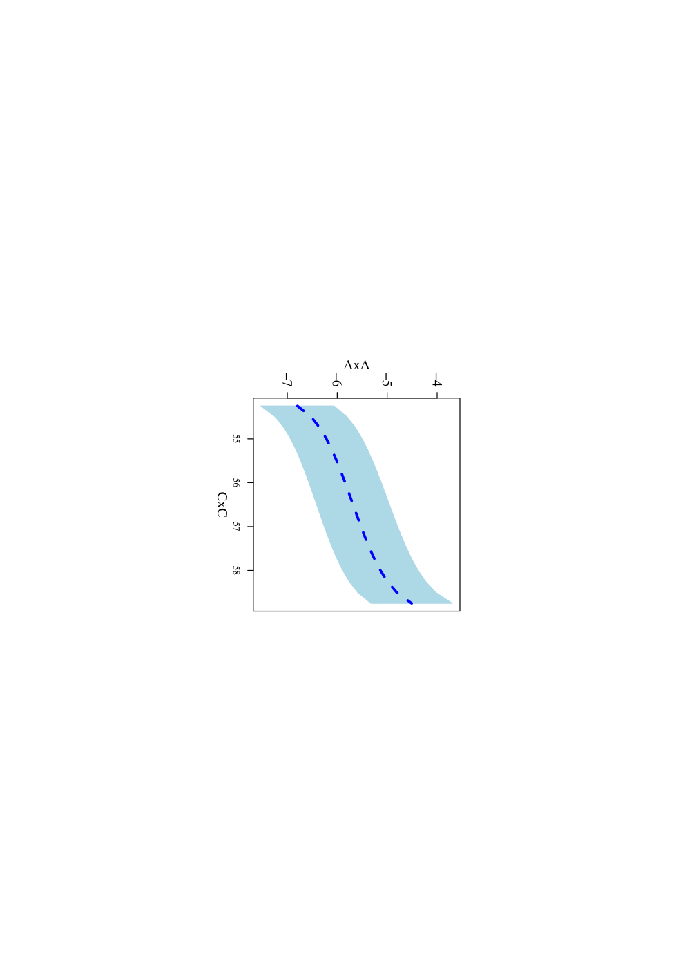
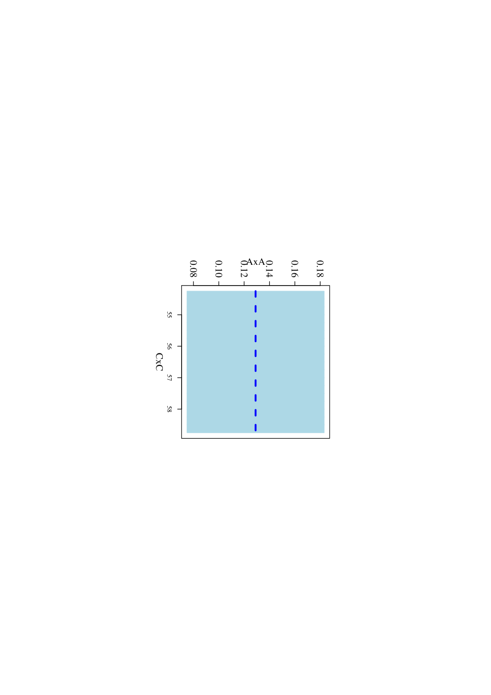
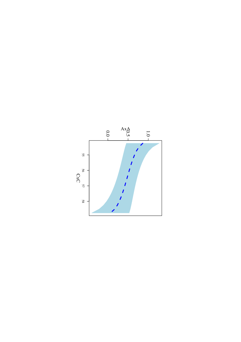
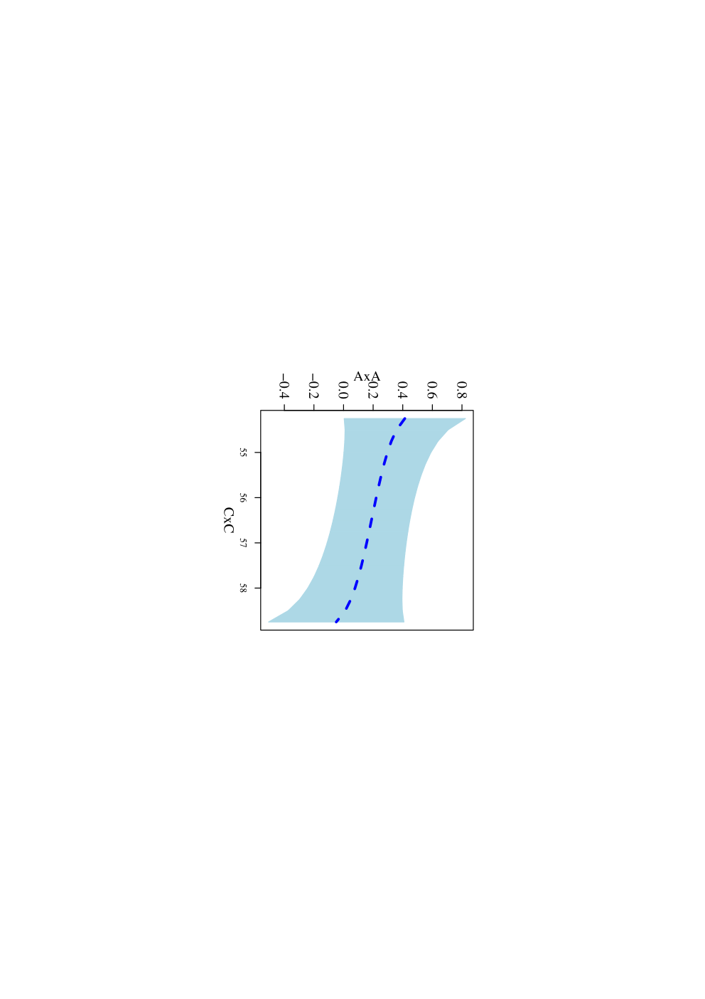
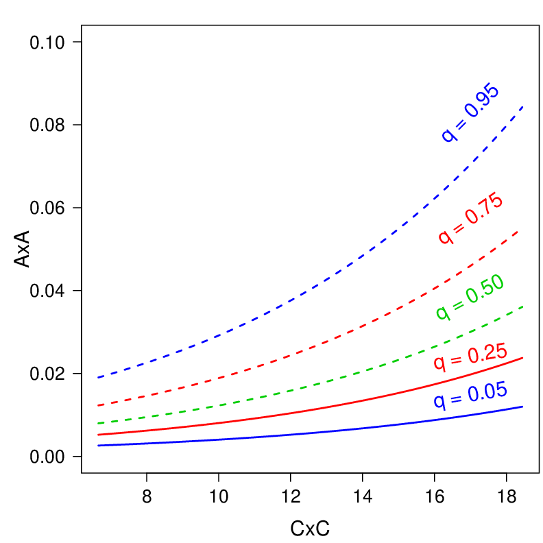
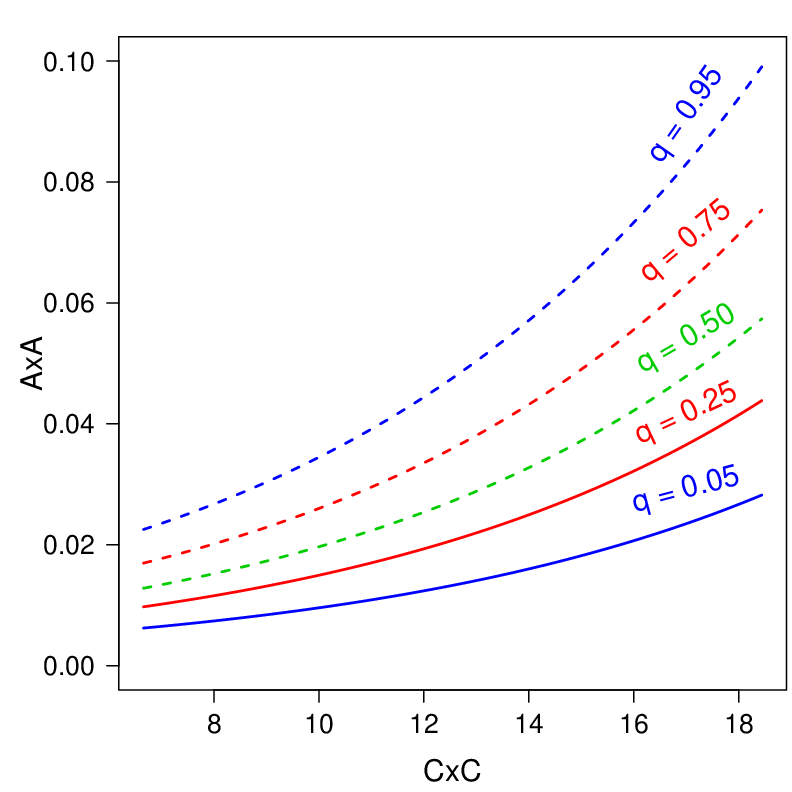
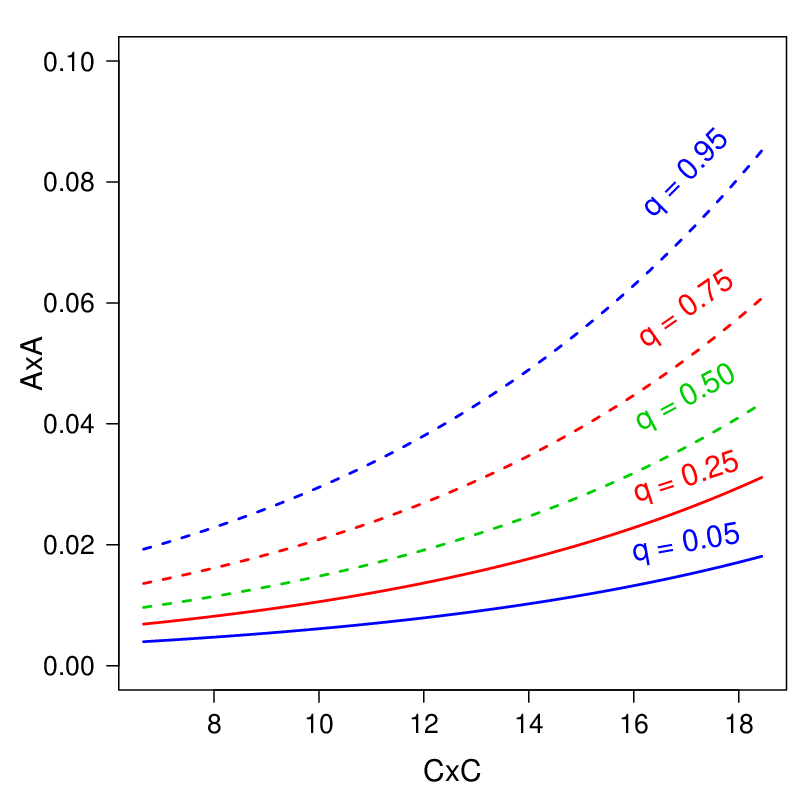
On the other hand, Figure 3 presented the point estimation and the 95% confidence interval (CI) for the parameters in terms of the quantile . From 3, the intercept for the quantile increases as increases, whereas the coefficients related to the quantile of America and Europe decreases when is increased. Furthermore, the coefficients related to the quantile for and the coefficients related to the scale of America and Europe remain similar for all . Figure 4 presented the estimated quantiles and for the mortality rate for different values of .
| -values for quantile residuals | |||||||||
|---|---|---|---|---|---|---|---|---|---|
| parameter | estimated | s.e. | -value | -value | KS | SW | AD | CVM | |
| -5.6835 | 0.3709 | -15.32 | 0.0001 | ||||||
| 0.1290 | 0.0276 | 4.68 | 0.0001 | ||||||
| 0.4749 | 0.1248 | 3.80 | 0.0001 | ||||||
| 0.50 | 0.1886 | 0.1320 | 1.43 | 0.0766 | 0.995 | 0.820 | 0.915 | 0.969 | |
| 0.9060 | 0.1556 | 5.82 | 0.0001 | ||||||
| 0.4294 | 0.2030 | 2.12 | 0.0172 | ||||||
| 0.2264 | 0.1737 | 1.30 | 0.0963 | ||||||
| 0.1164 | 0.3337 | 0.35 | 0.3636 | ||||||
5.1.2 Local influence analysis
We also presented a local influence analysis for the selected model under the three perturbations schemes discussed in Section 3.3. Figure 5 shows such analysis for the RPGJSB1 model with using the cloglog link and the cdf of the logistic model in the COVID-19 data set. In Section B.3 of the supplementary material is presented the same analysis for other selected quantiles. Note that, considering all the cases, the observation 121 appear in at least some case, which correspond to Yemen (Asia). Yemen reported a high mortality rate (29%, 601 accumulated deaths and 2067 accumulated cases, respectively). Evidently there is a problem in the handling of information about COVID-19 in the country. Table 6 presents the relative change for the parameters (RC), for its estimated standard errors (RCSE) and the respective p-value for the estimation without Yemen. We highlight that the greater variations are obtained for the parameters related to the scale and for (excepting the case for ). However, the estimated quantiles presented in Figure 3 do not depend on those parameters. Therefore, such plot without the referred observations are similar. We highlight that the significance of the parameters related to the quantile is maintained for all the cases (excepting for ), suggesting a robustness of the model to estimate the different quantiles in this problem.


| parameter | 0.10 | 0.25 | 0.50 | 0.75 | 0.90 | |
|---|---|---|---|---|---|---|
| RC | 7.81 | 11.06 | 16.43 | 23.58 | 32.58 | |
| RCSE | 0.20 | 0.10 | 0.05 | 0.27 | 0.66 | |
| p-value | 0.0001 | 0.0001 | 0.0001 | 0.0001 | 0.0001 | |
| RC | 15.58 | 15.58 | 15.58 | 15.58 | 15.58 | |
| RCSE | 0.28 | 0.28 | 0.28 | 0.28 | 0.28 | |
| p-value | 0.0001 | 0.0001 | 0.0001 | 0.0001 | 0.0001 | |
| RC | 1.17 | 13.45 | 41.56 | 99.46 | 266.08 | |
| RCSE | 4.83 | 7.63 | 8.81 | 2.12 | 28.95 | |
| p-value | 0.0003 | 0.0001 | 0.0001 | 0.0001 | 0.0001 | |
| RC | 9.43 | 30.59 | 78.19 | 216.11 | 2502.37 | |
| RCSE | 6.92 | 12.61 | 16.00 | 1.10 | 450.43 | |
| p-value | 0.0526 | 0.0431 | 0.0383 | 0.0359 | 0.0351 | |
| RC | 12.54 | 12.54 | 12.54 | 12.54 | 12.54 | |
| RCSE | 28.63 | 28.63 | 28.63 | 28.63 | 28.63 | |
| p-value | 0.0562 | 0.0562 | 0.0562 | 0.0562 | 0.0562 | |
| RC | 45.7 | 45.7 | 45.7 | 45.7 | 45.7 | |
| RCSE | 8.75 | 8.75 | 8.75 | 8.75 | 8.75 | |
| p-value | 0.1588 | 0.1588 | 0.1588 | 0.1588 | 0.1588 | |
| RC | 35.73 | 35.73 | 35.73 | 35.73 | 35.73 | |
| RCSE | 11.86 | 11.86 | 11.86 | 11.86 | 11.86 | |
| p-value | 0.3219 | 0.3219 | 0.3219 | 0.3219 | 0.3219 | |
| RC | 951.62 | 951.63 | 951.63 | 951.61 | 951.64 | |
| RCSE | 694.77 | 694.78 | 694.78 | 694.76 | 694.78 | |
| p-value | 0.3855 | 0.3855 | 0.3855 | 0.3855 | 0.3855 | |
6 Conclusions
In this paper, we propose two classes of parametric quantile regression models for studying the association between a bounded response and covariates via inferring the conditional quantile of the response. The proposed quantile regression models was built based on power Johnson SB distribution (Cancho et al. 2020) using a new parameterization of this distribution that is indexed by quantile, dispersion and shape parameters (RPGJSB1) or quantile and dispersion parameters (RPGJSB2). The first proposed quantile model has an extra-parameter is associated with the “tailedness”, and the second proposed quantile model has a less computational costs. The ML inference was implemented to estimate the models parameters, which was satisfactory considering the simulation studies where parameters were recovered for different sample sizes. Furthermore, under each proposed quantile regression model, we have developed model diagnostic tools. In order to illustrate our approach, two applications using real data sets were presented and discussed. In particular, we analyze the mortality rate of COVID-19 and the reproductive activity of the Chilean anchoveta. Results of the applications showed that the proposed quantile models are adequate. Based on the results, the RPGJSB1q regression model presents a better fit for the COVID-19 mortality rate and the anchoveta data sets. As part of future research, there are several extensions of the new models not considered in this paper that can be addressed in future research, in particular, an extension of the methods developed in this paper would be to consider in (2) a much more general family of distributions; that is, consider models for zero-inflated and one-inflated data set. Directions related to random effects in the model also can be addressed in future works.
Acknowledgements
The authors thank to “Instituto de fomento pesquero” (IFOP) to provide the anchoveta data set presented in the supplementary material.
References
- Bayes et al. (2012) Bayes, C.L., Bazán, J.L., García, C. (2012). A new robust regression model for proportions. Bayesian Analysis 7, 841-866.
- Bayes et al. (2017) Bayes, C.L., Bazán, J.L., De Castro, M.. (2017). A quantile parametric mixed regression model for bounded response variables. Statistics and Its Interface 10, 483-493.
- Cancho et al. (2020) Cancho, V.G., Bazán, J.L., Dey, D.K. (2020). A new class of regression model for a bounded response with application in the study of the incidence rate of colorectal cancer. Statistical Methods in Medical Research. 29, 2015-2033.
- Cook (1986) Cook, R. D. (1986). Assessment of Local Influence. Journal of the Royal Statistical Society: Series B (Methodological) 48, 133-155.
- Cox and Hinkley (1974) Cox, D. and Hinkley, D. (1974). Theoretical Statistics. Chapman and Hall, London, UK.
- Du et al. (2020) Du, R.H., Liang, L.R., Yang, C.Q., Wang, W., Cao, T.Z., Li, M., Guo, G.Y., Du, J., Zheng, C.L., Zhu, Q., Hu, M. (2020) Predictors of mortality for patients with COVID-19 pneumonia caused by SARS-CoV-2: a prospective cohort study. Eur. Respir. J., 55, 2000524
- Dunn and Smyth (1996) Dunn, P.K., Smyth, G.K. (1996). Randomized quantile residuals. Journal of Computational and Graphical Statistics 5, 236-244.
- Durrans (1992) Durrans, S.R. (1992). Distributions of fractional order statistics in hydrology. Water Resources Research 28, 1649-1655.
- Ferrari and Cribari-Neto (2004) Ferrari, S. L., Cribari-Neto, F. (2004). Beta regression for modelling rates and proportions. Journal of Applied Statistics 31, 799-815.
- Ji et al. (2020) Ji, J.S., Liu, Y., Liu, R., Zha, Y., Chang, X., Zhang, L., Zhang, Y., Zeng, J., Dong, T., Xu, X., Zhou, L. (2020) Survival analysis of hospital length of stay of novel coronavirus (COVID-19) pneumonia patients in Sichuan, China medRxiv (2020) 10.1101/2020.04.07.20057299
- Johnson (1949) Johnson, N.L. (1949). Systems of frequency curves generated by the methods of translation. Biometrika 36, 149-176.
- Koenker and Bassett (1978) Koenker, R., Bassett, G. (1978). Regression quantiles. Econometrica 46, 33-50.
- Lehmann (1953) Lehmann, E.L. (1953). The power of rank tests. Annals of Mathematical Statistics 24, 23-43.
- Lemonte and Bazán (2016) Lemonte, A.J., Bazán, J.L. (2016). New class of Johnson distributions and its associated regression model for rates and proportions. Biometrical Journal 58, 727-746.
- Lemonte and Moreno-Arenas (2020) Lemonte, A.J., Moreno-Arenas, G. (2020). On a heavy-tailed parametric quantile regression model for limited range response variables. Computational Statistics 35, 379-398.
- Livingston and Bucher (2020) Livingston, E., Bucher, K. (2020) Coronavirus disease 2019 (COVID-19) in Italy. Journal of the American Medical Association. 323, 1335.
- Li et al. (2020) Li, X., Xu, S., Yu, M., Wang, K., Tao, Y., Zhou, Y., Shi, J., Zhou, M., Wu, B., Yang, Z. (2020) Risk factors for severity and mortality in adult COVID-19 inpatients in Wuhan. J. Allergy Clin. Immunol. 146, 110-118
- Mazucheli et al. (2020) Mazucheli, J., Menezes, A.F.B., Fernandes, L.B., Oliveira, R.P., Ghitany, M.E. (2020). The unit- Weibull distribution as an alternative to the Kumaraswamy distribution for the modelling of quantiles conditional on covariates. Jounal of Applied Statistics 47, 954-974.
- Migliorati et al. (2018) Migliorati, S., Di Brisco, A.M., Ongaro, A. (2018). A New Regression Model for Bounded Responses. Bayesian Analysis 13, 845-872.
- Ospina and Ferrari (2008) Ospina, R., Ferrari, S.L.P. (2008). Inflated beta distributions. Statistical Papers 51, 111-126.
- Su (2015) Su, S. (2015). Flexible parametric quantile regression model. Statistics and Computing 25, 635-650.
- WHO (2020) WHO coronavirus disease (COVID-19) dashboard (2020). Geneva: World Health Organization. Available online: https://covid19.who.int/ (last cited: [03/11/2020]).
- Yap and Sim (2011) Yap, B.W., Sim, C.H. (2011) Comparisons of various normality tests. Journal of Statistical Computation and Simulation 81, 2141-2155.