跳到论文正文
W Papers独立论文阅读器 arXiv:2103.06923 论文正文 计算阅读时间 · 0%
引用这篇论文根据当前论文元数据生成,正式投稿前建议核对。


License: arXiv.org perpetual non-exclusive license
arXiv:2103.06923v2 [math.ST] 16 Mar 2021

Non-Asymptotic Performance Guarantees for
Neural Estimation of 𝖿\mathsf{f}-Divergences

Sreejith Sreekumar    Zhengxin Zhang    Ziv Goldfeld
Abstract

Statistical distances (SDs), which quantify the dissimilarity between probability distributions, are central to machine learning and statistics. A modern method for estimating such distances from data relies on parametrizing a variational form by a neural network (NN) and optimizing it. These estimators are abundantly used in practice, but corresponding performance guarantees are partial and call for further exploration. In particular, there seems to be a fundamental tradeoff between the two sources of error involved: approximation and estimation. While the former needs the NN class to be rich and expressive, the latter relies on controlling complexity. This paper explores this tradeoff by means of non-asymptotic error bounds, focusing on three popular choices of SDs—Kullback-Leibler divergence, chi-squared divergence, and squared Hellinger distance. Our analysis relies on non-asymptotic function approximation theorems and tools from empirical process theory. Numerical results validating the theory are also provided.

†† The work of S. Sreekumar is supported by the TRIPODS Center for Data Science National Science Foundation Grant CCF-1740822. The work of Z. Goldfeld is supported in part by the NSF CRII Award under Grant CCF-1947801, in part by the 2020 IBM Academic Award, and in part by the NSF CAREER Award under Grant CCF-2046018. S. Sreekumar and Z. Goldfeld are with the School of Electrical and Computer Engineering, Cornell University, Ithaca, NY 14850, USA. Z. Zhang is with the Center for Applied Mathematics at the same University. (email: sreejithsreekumar@cornell.edu; zz658@cornell.edu; goldfeld@cornell.edu).

I INTRODUCTION

Statistical distances (SDs) measure the discrepancy between probability distributions. A variety of machine learning (ML) tasks, from generative modeling (Kingma and Welling 2014; Goodfellow et al. 2014; Nowozin et al. 2016; Arjovsky et al. 2017; Tolstikhin et al. 2018) to those relying on barycenters (Rabin et al. 2011; Gramfort et al. 2015; Dognin et al. 2019), can be posed as measuring or optimizing a SD between the data distribution and the model. Popular SDs include 𝖿\mathsf{f}-divergences (Ali and Silvey 1966; Csiszár 1967), integral probability metrics (IPMs) (Zolotarev 1983; Müller 1997), and Wasserstein distances (Villani 2008). A common formulation that captures many of these is11 1 Specifically, (1) accounts for 𝖿\mathsf{f}-divergences, IPMs and the 1-Wasserstein distance.

𝖧γ,ℱ​(P,Q)=supf∈ℱ𝔼P​[f]−𝔼Q​[γ∘f],\mathsf{H}_{\gamma,\mathcal{F}}(P,Q)=\sup_{f\in\mathcal{F}}\mathbb{E}_{P}[f]-\mathbb{E}_{Q}[\gamma\circ f], (1)

where ℱ\mathcal{F} is a function class of ‘discriminators’ and γ\gamma is sometimes called a ‘measurement function’ (cf., e.g., Arora et al. 2017). This variational form is at the core of many ML algorithms implemented based on SDs, and has been recently leveraged for estimating SDs from samples.

Various non-parametric estimators of SDs are available in the literature (Wang et al. 2005; Perez-Cruz 2008; Krishnamurthy et al. 2014; Kandasamy et al. 2015; Liang 2019). These classic methods typically rely on kernel density estimation (KDE) or kk-nearest neighbors (kNN) techniques, and are known to achieve optimal estimation error rates for specific SDs, subject to smoothness and/or regularity conditions on the densities. To mention a few, Kandasamy et al. 2015 proposed a KDE-based estimator which achieves the parametric mean squared error (MSE) rate for KL divergence estimation, provided that the densities are bounded away from zero and belong to a Hölder class of sufficiently large smoothness. For the special case of entropy estimation in the high smoothness regime, Berrett et al. 2019 proposed an asymptotically efficient weighted kNN estimator that does not rely on the boundedness from below assumption. Recently, Han et al. 2020 proposed a minimax rate-optimal entropy estimator for densities of sufficient Lipschitz smoothness. While these classic estimators achieve optimal performance under appropriate assumptions, they are often hard to compute in high dimensions.

I-A Statistical Distances Neural Estimation

Typical applications to machine learning, e.g., generative adversarial networks (GANs) (Nowozin et al. 2016; Arjovsky et al. 2017) or anomaly detection (Póczos et al. 2011), favor estimators whose computation scales well with number of samples and is compatible with backpropagation and minibatch-based optimization. A modern estimation technique that adheres to these requirements is the so-called neural estimation method (Arora et al. 2017; Zhang et al. 2018; Belghazi et al. 2018). Neural estimators (NEs) parameterize the discriminator class ℱ\mathcal{F} in (1) by a neural network (NN), approximate expectations by sample means, and then optimize the obtained empirical objective. Denoting the samples from PP and QQ by Xn:=(X1,⋯,Xn)X^{n}:=(X_{1},\cdots,X_{n}) and Yn:=(Y1,⋯,Yn)Y^{n}:=(Y_{1},\cdots,Y_{n}), respectively, the resulting NE is

𝖧^γ,𝒢k​(Xn,Yn):=supg∈𝒢k1n​∑i=1n[g⁡(Xi)−γ∘g⁡(Yi)],\hat{\mathsf{H}}_{\gamma,\mathcal{G}_{k}}(X^{n},Y^{n}):=\sup_{g\in\mathcal{G}_{k}}\frac{1}{n}\sum_{i=1}^{n}\Big[g(X_{i})-\gamma\circ g(Y_{i})\Big], (2)

where 𝒢k\mathcal{G}_{k} is the class of functions realizable by a kk-neuron NN. Despite the popularity of NEs in applications, their theoretical properties and corresponding performance guarantees remain largely obscure. Addressing this deficit is the objective of this work.

There is a fundamental tradeoff between the quality of approximation by NNs and the sample size needed for accurate estimation of the parametrized form. The former is measured by the approximation error, |𝖧γ,ℱ​(P,Q)−𝖧γ,𝒢k​(P,Q)|\big|\mathsf{H}_{\gamma,\mathcal{F}}(P,Q)-\mathsf{H}_{\gamma,\mathcal{G}_{k}}(P,Q)\big|, whereas the latter by the estimation error, |𝖧^γ,𝒢k​(Xn,Yn)−𝖧γ,𝒢k​(P,Q)|\big|\hat{\mathsf{H}}_{\gamma,\mathcal{G}_{k}}(X^{n},Y^{n})-\mathsf{H}_{\gamma,\mathcal{G}_{k}}(P,Q)\big|. While approximation needs 𝒢k\mathcal{G}_{k} to be rich and expressive, efficient estimation relies on controlling its complexity. Past works on NEs provide only a partial account of estimation performance. Belghazi et al. 2018 proved consistency of mutual information neural estimation (MINE), which boils down to estimating KL divergence, but do not quantify approximation errors. Non-asymptotic sample complexity bounds for the parameterized form, i.e., when ℱ\mathcal{F} in (1) is the NN class 𝒢k\mathcal{G}_{k} to begin with, were derived in Arora et al. 2017; Zhang et al. 2018. These objects are known as NN distances and, by definition, overlook the approximation error with respect to (w.r.t.) the original SD. Also related is Nguyen et al. 2010, where KL divergence estimation rates are provided under the assumption that the approximating class is large enough to contain an optimizer of (1). This assumption is often violated in practice, e.g., when using NNs as done herein, or a reproducing kernel Hilbert space, as considered in Nguyen et al. 2010. This makes the quantification of the approximation error pivotal for a complete account of estimation performance. In light of the above, our objective is to derive non-asymptotic neural estimation performance bounds that characterize the dependence of the error on kk and nn, and help understand tradeoffs between them.

I-B Contributions

We show that the effective (approximation plus estimation) error of a NE realized by a kk-neuron shallow NN with bounded parameters and nn samples scales like

O(k−1/2+hγ(k)n−1/2),O\left(k^{-1/2}+h_{\gamma}(k)n^{-1/2}\right),

where hγ​(k)h_{\gamma}(k) grows with kk at a rate that depends on the estimated SD. In order to bound the approximation error, we refine Theorem 1 in Barron 1992 to show that a kk-neuron NN with bounded parameters can approximate any function in the Barron class (Barron 1993) under the sup-norm within an O(k−1/2)O(k^{-1/2}) error. To control the empirical estimation error, we leverage tools from empirical process theory and bound the associated entropy integral (Van Der Vaart and Wellner 1996) to achieve the O(hγ(k)n−1/2)O\left(h_{\gamma}(k)n^{-1/2}\right) convergence rate.

The effective error bound is then specialized to three predominant 𝖿\mathsf{f}-divergences: KL, chi-squared (χ2\chi^{2} divergence, and squared Hellinger distance. We establish finite-sample absolute-error bounds of these NEs by identifying the appropriate scaling of the width kk with the sample size nn in the general bounds. This, in turn, implies consistency of the NEs. Our analysis is based on two key observations. First, to achieve a small approximation error, we would like 𝒢k\mathcal{G}_{k} to universally approximate the original function class ℱ\mathcal{F}, which needs either width (Lu et al. 2017) or parameters (Stinchcombe and White 1990) to be unbounded. On the other hand, to achieve the parametric estimation rate n−1/2n^{-1/2}, the class 𝒢k\mathcal{G}_{k} must not be too large. The effective error bound then relies on finding the appropriate scaling of kk (and the uniform parameter norm) with nn so that a small approximation error and fast estimation rates are both attained. Numerical results (on synthetic data) validating our theory are also provided.

I-C Notation

Let ∥⋅∥\|\cdot\| denote the Euclidean norm on ℝd\mathbb{R}^{d}, and x⋅yx\cdot y designate the inner product. The Euclidean ball of radius r≥0r\geq 0 centered at 0 is Bd​(r)B^{d}(r). We use ℝ¯:=ℝ∪{−∞,∞}\bar{\mathbb{R}}:=\mathbb{R}\cup\{-\infty,\infty\} for the extended reals. For 1≤p<∞1\leq p<\infty, the LpL^{p} space over 𝒳⊆ℝd\mathcal{X}\subseteq\mathbb{R}^{d} w.r.t. the Lebesgue measure is denoted by Lp​(𝒳)L^{p}(\mathcal{X}), with ∥⋅∥p\|\cdot\|_{p} designating the norm. We let (Ω,𝒜,ℙ)(\Omega,\mathcal{A},\mathbb{P}) be the probability space on which all random variables are defined; 𝔼\mathbb{E} denotes the corresponding expectation. The class of Borel probability measures on 𝒳⊆ℝd\mathcal{X}\subseteq\mathbb{R}^{d} is denoted by 𝒫⁡(𝒳)\mathcal{P}(\mathcal{X}). To stress that an expectation of ff is taken w.r.t. P∈𝒫⁡(𝒳)P\in\mathcal{P}(\mathcal{X}), we write 𝔼P​[f]\mathbb{E}_{P}[f]. We assume that all functions considered henceforth are Borel functions. The essential supremum of a function w.r.t. P∈𝒫⁡(𝒳)P\in\mathcal{P}(\mathcal{X}) is denoted by 𝖾𝗌𝗌​𝗌𝗎𝗉P​(f)\mathsf{ess\,sup}_{P}(f). For P,Q∈𝒫⁡(𝒳)P,Q\in\mathcal{P}(\mathcal{X}) with P≪QP\ll Q, i.e., PP is absolutely continuous w.r.t. QQ, we use 𝖽​P𝖽​Q\frac{\,\mathsf{d}P}{\,\mathsf{d}Q} for the Radon-Nikodym derivative of PP w.r.t. QQ. For n∈ℕn\in\mathbb{N}, P⊗nP^{\otimes n} denotes the nn-fold product measure of PP. For an open set 𝒰⊆ℝd\mathcal{U}\subseteq\mathbb{R}^{d} and an integer m≥0m\geq 0, the class of functions such that all partial derivatives of order mm exist and are continuous on 𝒰\mathcal{U} are denoted by 𝖢m​(𝒰)\mathsf{C}^{m}(\mathcal{U}). In particular, 𝖢​(𝒰):=𝖢0​(𝒰)\mathsf{C}(\mathcal{U}):=\mathsf{C}^{0}(\mathcal{U}) and 𝖢∞​(𝒰)\mathsf{C}^{\infty}(\mathcal{U}) denotes the class of continuous functions and infinitely differentiable functions on 𝒰\mathcal{U}. The restriction of a function f:ℝd→ℝf:\mathbb{R}^{d}\to\mathbb{R} to a subset 𝒳⊆ℝd\mathcal{X}\subseteq\mathbb{R}^{d} is represented by f|𝒳f|_{\mathcal{X}}. For a,b∈ℝa,b\in\mathbb{R}, a∨b:=max⁡{a,b}a\vee b:=\max\{a,b\} and a∧b:=min⁡{a,b}a\wedge b:=\min\{a,b\}. For a multi-index 𝜶=(α1,⋯,αd)\bm{\alpha}=(\alpha_{1},\cdots,\alpha_{d}), D𝜶:=∂α1∂α1x1⋯∂αd∂αdxdD^{\bm{\alpha}}:=\frac{\partial^{\alpha_{1}}}{\partial^{\alpha_{1}}x_{1}}\cdots\frac{\partial^{\alpha_{d}}}{\partial^{\alpha_{d}}x_{d}} denotes the partial derivative operator of order |𝜶|:=∑j=1dαj\left|\bm{\alpha}\right|:=\sum_{j=1}^{d}\alpha_{j}.

II Background and Preliminaries

Below, we provide a short background on the central technical ideas used in the paper.

Statistical distances.

A common variational formulation of a SDs between P,Q∈𝒫⁡(𝒳)P,Q\in\mathcal{P}(\mathcal{X}), 𝒳⊆ℝd\mathcal{X}\subseteq\mathbb{R}^{d}, is

𝖧γ,ℱ​(P,Q)=supf∈ℱ𝔼P​[f]−𝔼Q​[γ∘f],\displaystyle\mathsf{H}_{\gamma,\mathcal{F}}(P,Q)=\sup_{f\in\mathcal{F}}\mathbb{E}_{P}[f]-\mathbb{E}_{Q}[\gamma\circ f], (3)

where γ:ℝ→ℝ¯\gamma:\mathbb{R}\rightarrow\bar{\mathbb{R}}, and ℱ\mathcal{F} is a class of measurable functions f:ℝd→ℝf:\mathbb{R}^{d}\rightarrow\mathbb{R} for which the expectations are finite. This formulation captures 𝖿\mathsf{f}-divergences (when γ\gamma is the convex conjugate of OPEN𝖿)\mathsf{f}), IPMs (for γ⁡(x)=x\gamma(x)=x) as well as the 1-Wasserstein distance (which is an IPM w.r.t. the 1-Lipschitz function class).

𝒢k(𝐚):={g:ℝd→ℝ:g(x)=∑i=1kβiϕ(wi⋅x+bi)+b0,wi∈ℝd,b0,bi,βi∈ℝ,maxi=1,…,kj=1,…,d{|wi,j|,|bi|}≤a1,|βi|≤a2,i=1,…,k,|b0|≤a3}.\mathcal{G}_{k}(\mathbf{a}):=\mspace{-3mu}\left\{g:\mathbb{R}^{d}\mspace{-5mu}\rightarrow\mathbb{R}:\begin{aligned} &g(x)=\sum_{i=1}^{k}\beta_{i}\phi\left(w_{i}\cdot x+b_{i}\right)+b_{0},~w_{i}\in\mathbb{R}^{d},~b_{0},b_{i},\beta_{i}\in\mathbb{R},\\ &\max\nolimits_{\begin{subarray}{c}i=1,\ldots,k\\ j=1,\ldots,d\end{subarray}}\left\{|w_{i,j}|,|b_{i}|\right\}\leq a_{1},~|\beta_{i}|\leq a_{2},~~i=1,\ldots,k,~|b_{0}|\leq a_{3}\end{aligned}\right\}\mspace{-3mu}. (11)


Approximated function class.

Our approximation result requires the target function with domain 𝒳\mathcal{X} to have an extension on ℝd\mathbb{R}^{d}, which belongs to a certain class of functions introduced in Barron 1993.

Definition 1 (Barron class).

Consider a function f:ℝd→ℝf:\mathbb{R}^{d}\rightarrow\mathbb{R} that has a Fourier representation f⁡(x)=∫0∞ei​ω⋅x​F~​(𝑑ω)f(x)=\int_{0}^{\infty}e^{i\omega\cdot x}\tilde{F}(d\omega), where F~​(d​ω)\tilde{F}(d\omega) is a complex Borel measure over ℝd\mathbb{R}^{d} with magnitude F⁡(d​ω)F(d\omega) that satisfies

B⁡(f,𝒳):=∫ℝdsupx∈𝒳|ω⋅x|​F​(𝑑ω)<∞.B(f,\mathcal{X}):=\int_{\mathbb{R}^{d}}\sup_{x\in\mathcal{X}}\left|\omega\cdot x\right|F(d\omega)<\infty. (4)

For c≥0c\geq 0, the Barron class is

ℬc(𝒳):={f:ℝd→ℝ,B(f,𝒳)∨|f(0)|≤c}.\displaystyle\mathcal{B}_{c}(\mathcal{X})\mspace{-4mu}:=\mspace{-4mu}\left\{f:\mathbb{R}^{d}\rightarrow\mathbb{R},B(f,\mathcal{X})\vee\left|f(0)\right|\mspace{-3mu}\leq\mspace{-3mu}c\right\}. (5)

For f~:𝒳→ℝ\tilde{f}:\mathcal{X}\rightarrow\mathbb{R}, define

cB⋆(f~,𝒳):=inf{c:∃f∈ℬc(𝒳),f~=f|𝒳}.\displaystyle c_{B}^{\star}(\tilde{f},\mathcal{X}):=\mspace{-4mu}\inf\left\{c:\exists~f\in\mathcal{B}_{c}(\mathcal{X}),~\tilde{f}=f|_{\mathcal{X}}\right\}. (6)
Stochastic processes.

Our analysis of the estimation error requires the following definitions.

Definition 2 (Subgaussian process).

Let (Θ,d)(\Theta,d) be a metric space. A real-valued stochastic process {Xθ}θ∈Θ\{X_{\theta}\}_{\theta\in\Theta} with index set Θ\Theta is called subgaussian if it is centered and

𝔼⁡[et⁡(Xθ−Xθ′)]≤e12​t2​d​(θ,θ′)2,∀θ,θ′∈Θ,t≥0.\mathbb{E}\big[e^{t(X_{\theta}-X_{\theta^{\prime}})}\big]\leq e^{\frac{1}{2}t^{2}d(\theta,\theta^{\prime})^{2}},~\forall~\theta,\theta^{\prime}\in\Theta,~t\geq 0. (7)
Definition 3 (Separable process).

A stochastic process {Xθ}θ∈Θ\{X_{\theta}\}_{\theta\in\Theta} on a metric space (Θ,d)(\Theta,d) is called separable if there exists a countable set Θ0⊆Θ\Theta_{0}\subseteq\Theta, such that

limθ′→θ:θ′∈Θ0Xθ′→Xθ,∀θ∈Θa.s.\displaystyle\lim_{\theta^{\prime}\rightarrow\theta:\ \theta^{\prime}\in\Theta_{0}}X_{\theta^{\prime}}\rightarrow X_{\theta},~\forall~\theta\in\Theta\qquad\mbox{a.s.} (8)
Definition 4 (Covering number).

A set Θ′\Theta^{\prime} is an ϵ\epsilon-covering for the metric space (Θ,d)(\Theta,d) if for every θ∈Θ\theta\in\Theta, there exists a θ′∈Θ′\theta^{\prime}\in\Theta^{\prime} such that d⁡(θ,θ′)≤ϵd(\theta,\theta^{\prime})\leq\epsilon. The ϵ\epsilon-covering number is

N⁡(Θ,d,ϵ):=inf{|Θ′|:Θ′​ is an ​ϵ​-covering for ​Θ}.N(\Theta,d,\epsilon):=\inf\left\{|\Theta^{\prime}|:~\Theta^{\prime}\mbox{ is an }\epsilon\mbox{-covering for }\Theta\right\}.

The next theorem gives a tail bound for the supremum of a subgaussian process in terms of the covering number. This result is key for our estimation error analysis.

Theorem 1.

(van Handel 2016, Theorem 5.29) Let {Xθ}θ∈Θ\{X_{\theta}\}_{\theta\in\Theta} be a separable subgaussian process on the metric space (Θ,d)(\Theta,d). Then, for any θ0∈Θ\theta_{0}\in\Theta and δ≥0\delta\geq 0, we have

ℙ⁡(supθ∈ΘXθ−Xθ0≥C​∫0∞log⁡N⁡(Θ,d,ϵ)​𝑑ϵ+δ)\displaystyle\mathbb{P}\left(\sup_{\theta\in\Theta}X_{\theta}-X_{\theta_{0}}\geq C\int_{0}^{\infty}\sqrt{\log N(\Theta,d,\epsilon)}d\epsilon+\delta\right)
≤C​e−δ2C​𝖽𝗂𝖺𝗆​(Θ)2,\displaystyle\leq Ce^{-\frac{\delta^{2}}{C\mathsf{diam}(\Theta)^{2}}}, (9)

for 𝖽𝗂𝖺𝗆⁡(Θ):=supθ,θ′∈Θd⁡(θ,θ′)\mathsf{diam}(\mspace{-1.5mu}\Theta\mspace{-1.5mu})\mspace{-3mu}:=\mspace{-8mu}\sup\limits_{\theta,\theta^{\prime}\in\Theta}\mspace{-6mu}d(\mspace{-1mu}\theta\mspace{-3mu},\mspace{-2mu}\theta^{\prime}\mspace{-1mu}) and a universal constant CC.

ℋb,cl,δ(𝒰):={f∈𝖢l(𝒰):|D𝜶​f​(x)−D𝜶​f​(x′)|≤c​‖x−x′‖δ,∀x,x′∈𝒰,|𝜶|=l,max𝜶:|𝜶|≤lsupx∈𝒰|D𝜶f(x)|≤b}.\mathcal{H}_{b,c}^{l,\delta}(\mathcal{U}):=\left\{f\in\mathsf{C}^{l}(\mathcal{U}):\ \ \begin{aligned} &\left|D^{\bm{\alpha}}f(x)-D^{\bm{\alpha}}f(x^{\prime})\right|\leq c\left\|x-x^{\prime}\right\|^{\delta},~\forall x,x^{\prime}\in\mathcal{U},~\left|\bm{\alpha}\right|=l,\\ &\max_{\bm{\alpha}:\left|\bm{\alpha}\right|\leq l}\sup_{x\in\mathcal{U}}\left|D^{\bm{\alpha}}f(x)\right|\leq b\end{aligned}\right\}. (14)


III Statistical Distances Neural Estimation

For simplicity of presentation, we henceforth fix 𝒳=[0,1]d\mathcal{X}=[0,1]^{d}, although our results and analysis readily generalize to arbitrary compact supports 𝒳⊂ℝd\mathcal{X}\subset\mathbb{R}^{d}. Accordingly, B⁡(f,𝒳)B(f,\mathcal{X}), ℬc​(𝒳)\mathcal{B}_{c}(\mathcal{X}) and cB⋆​(f~,𝒳)c_{B}^{\star}(\tilde{f},\mathcal{X}) are denoted by B⁡(f)B(f), ℬc\mathcal{B}_{c} and cB⋆​(f~)c_{B}^{\star}(\tilde{f}), respectively. We first describe the neural estimation method, followed by two technical results that account for the approximation and the estimation errors. These results are later leveraged to derive effective error bounds for neural estimation of KL and χ2\chi^{2} divergences, as well as the squared Hellinger distance. All proofs are deferred to the supplement.

III-A Neural Estimation

Let P,Q∈𝒫⁡(𝒳)P,Q\in\mathcal{P}(\mathcal{X}). Consider a SD 𝖧γ,ℱ​(P,Q)\mathsf{H}_{\gamma,\mathcal{F}}(P,Q) between these distributions (see (3)), and assume that nn independently and identically distributed (i.i.d.) samples Xn:=(X1,⋯,Xn)X^{n}:=(X_{1},\cdots,X_{n}) and Yn:=(Y1,⋯,Yn)Y^{n}:=(Y_{1},\cdots,Y_{n}) from PP and QQ, respectively, are available. The NE of 𝖧γ,ℱ​(P,Q)\mathsf{H}_{\gamma,\mathcal{F}}(P,Q) based on a kk-neuron shallow network (to parametrize the function class ℱ\mathcal{F}) and the samples Xn,YnX^{n},Y^{n} (to approximate the expected values) is

𝖧^γ,𝒢k​(𝐚)​(Xn,Yn):=supg∈𝒢k​(𝐚)1n​∑i=1n[g⁡(Xi)−γ∘g⁡(Yi)],\hat{\mathsf{H}}_{\gamma,\mathcal{G}_{k}(\mathbf{a})}(X^{n},Y^{n})\mspace{-3mu}:=\mspace{-5mu}\sup_{g\in\mathcal{G}_{k}(\mathbf{a})}\frac{1}{n}\sum_{i=1}^{n}\mspace{-3mu}\Big[g(X_{i})-\gamma\circ g(Y_{i})\Big], (10)

where 𝒢k​(𝐚)\mathcal{G}_{k}(\mathbf{a}) is the NN class defined in (11) above, with parameter bounds specified by 𝐚=(a1,a2,a3)\mathbf{a}=(a_{1},a_{2},a_{3}) ∈ℝ≥03\in\mathbb{R}^{3}_{\geq 0}, and activation function ϕ:ℝ→ℝ\phi:\mathbb{R}\rightarrow\mathbb{R}, which is henceforth taken as the logistic sigmoid ϕ⁡(x)=11+e−x\phi(x)=\frac{1}{1+e^{-x}}. The results that follow extend to any measurable bounded variation sigmoidal (i.e., ϕ⁡(z)→1\phi(z)\rightarrow 1 as z→∞z\rightarrow\infty and ϕ⁡(z)→0\phi(z)\rightarrow 0 as z→−∞z\rightarrow-\infty) activation.

Our goal is to provide absolute-error performance guarantees for this NE, in terms of the approximation error and the statistical estimation error.22 2 In practice, an optimization error is also present, but its exploration is left for future work.

III-B Sup-norm Function Approximation

We start with a bound on the approximation error of a target function f~\tilde{f} with domain 𝒳\mathcal{X} for which cB⋆​(f~)<∞c_{B}^{\star}(\tilde{f})<\infty.

Theorem 2 (Approximation).

Let P,Q∈𝒫⁡(𝒳)P,Q\in\mathcal{P}(\mathcal{X}) and consider the NN class 𝒢k∗​(c):=𝒢k​(k​log⁡k,2​k−1​c,c)\mathcal{G}_{k}^{*}\left(c\right):=\mathcal{G}_{k}\left(\sqrt{k}\log k,2k^{-1}c,c\right) (see (11)) for some c≥0c\geq 0. Given f~:𝒳→ℝ\tilde{f}:\mathcal{X}\rightarrow\mathbb{R} such that cB⋆​(f~)≤cc_{B}^{\star}(\tilde{f})\leq c, there exists g∈𝒢k∗​(c)g\in\mathcal{G}_{k}^{*}\left(c\right) satisfying

‖f~−g‖∞,P,Q=O⁡(k−12),\displaystyle\big\|\tilde{f}-g\big\|_{\infty,P,Q}=O\left(k^{-\frac{1}{2}}\right),\vskip-8.53581pt (12)

where ‖f−g‖∞,P,Q:=𝖾𝗌𝗌​𝗌𝗎𝗉P​|f−g|∨𝖾𝗌𝗌​𝗌𝗎𝗉Q​|f−g|\left\|f\mspace{-3mu}-\mspace{-3mu}g\right\|_{\infty,P,Q}\mspace{-3mu}:=\mathsf{ess\,sup}_{P}|f\mspace{-1.5mu}-\mspace{-1.5mu}g|\vee\mathsf{ess\,sup}_{Q}|f\mspace{-1.5mu}-\mspace{-1.5mu}g|. Moreover, for any 𝐚∈ℝ≥03\mathbf{a}\in\mathbb{R}^{3}_{\geq 0}, c>0c>0, and ϵ>0\epsilon>0, there exists f~:𝒳→ℝ\tilde{f}:\mathcal{X}\rightarrow\mathbb{R} with cB⋆​(f~)≤cc_{B}^{\star}(\tilde{f})\leq c such that

infg∈𝒢k​(𝐚)‖f~−g‖2=Ω⁡(k−(12+1d+ϵ)).\displaystyle\inf_{g\in\mathcal{G}_{k}(\mathbf{a})}\big\|\tilde{f}-g\big\|_{2}=\Omega\left(k^{-\big(\frac{1}{2}+\frac{1}{d}+\epsilon\big)}\right).\vskip-8.53581pt (13)

The explicit dependence of dd and cc in the right hand side (R.H.S.) of (12) is given in (42).

The above theorem states that a kk-neuron shallow NN can approximate a function f~\tilde{f} on 𝒳\mathcal{X} within an O(k−1/2)O(k^{-1/2}) gap in the uniform norm, provided f~\tilde{f} is the restriction of some ff from the Barron class. The upper and lower bounds in (12) and (13) differ by k−(1/d+ϵ)k^{-(1/d+\epsilon)}, which becomes negligible for large dd and small ϵ\epsilon. Also observe that the lower bound is in terms of L2L^{2} norm which implies a lower bound w.r.t. the L∞L^{\infty} norm.

Remark 1 (Relation to previous results).

A result reminiscent to Theorem 2 appears in Barron 1992, but some technical details had to be adapted to apply the bound to neural estimation of SDs. Theorem 2 generalizes Barron 1992 and Yukich et al. 1995 from unbounded NN weights and bias parameters to bounded ones. We note that while Yukich et al. 1995 allows unbounded parameters (input weight and bias), a more general problem of approximating a function and its derivatives is treated therein. Here we only consider the approximation of the function itself.

We next show that a sufficiently smooth Hölder function on 𝒳\mathcal{X} is the restriction of some function in the Barron class. To that end we first define the Hölder function class.

Definition 5 (Holder class).

For b,c,δ≥0b,c,\delta\geq 0, an integer l≥0l\geq 0, and an open set 𝒰⊆ℝd\mathcal{U}\subseteq\mathbb{R}^{d}, the bounded holder class ℋb,cl,δ​(𝒰)\mathcal{H}_{b,c}^{l,\delta}(\mathcal{U}) is defined in (14) above.

We have the following universal approximation property for Hölder functions.

Corollary 1 (Approximation of Hölder functions).

Given a function f~:𝒳→ℝ\tilde{f}:\mathcal{X}\rightarrow\mathbb{R}, suppose there exists an open set 𝒰⊃𝒳~\mathcal{U}\supset\mathcal{X}, b,c,δ≥0b,c,\delta\geq 0, and f∈ℋb,cs,δ​(𝒰)f\in\mathcal{H}_{b,c}^{s,\delta}(\mathcal{U}), s:=⌊d2⌋+2s:=\lfloor\frac{d}{2}\rfloor+2, such that f~=f|𝒳\tilde{f}=f|_{\mathcal{X}}. Then, there exists g∈𝒢k∗​(c¯b,c,d)g\in\mathcal{G}_{k}^{*}\left(\bar{c}_{b,c,d}\right) such that

‖f~−g‖∞,P,Q=O⁡(k−12),\displaystyle\vskip-11.38109pt\big\|\tilde{f}-g\big\|_{\infty,P,Q}=O\left(k^{-\frac{1}{2}}\right),\vskip-11.38109pt (15)

where c¯b,c,d\bar{c}_{b,c,d} is given in (54) in Appendix A-B.

III-C Estimation of Parameterized Distances

We next bound the error of estimating the parametrized SD 𝖧γ,𝒢k​(𝐚)​(P,Q)\mathsf{H}_{\gamma,\mathcal{G}_{k}(\mathbf{a})}(P,Q) (i.e., (3) for a NN function class) by its empirical version from (10). Throughout this section we assume that XnX^{n} and YnY^{n} are, respectively, i.i.d. samples from PP and QQ.

Theorem 3 (Empirical estimation error tail bound).

Let P,Q∈𝒫⁡(𝒳)P,Q\in\mathcal{P}(\mathcal{X}). Assume that 𝐚∈ℝ≥03\mathbf{a}\in\mathbb{R}^{3}_{\geq 0}, 𝒢k​(𝐚)\mathcal{G}_{k}(\mathbf{a}), and γ:ℝ→ℝ¯\gamma:\mathbb{R}\to\bar{\mathbb{R}} are such that 𝖧γ,𝒢k​(𝐚)​(P,Q)<∞\mathsf{H}_{\gamma,\mathcal{G}_{k}(\mathbf{a})}(P,Q)<\infty and

γ¯𝒢k​(𝐚)′:=supx∈𝒳,g∈𝒢k​(𝐚)γ′∘g⁡(x)<∞,\displaystyle\bar{\gamma}^{\prime}_{\mathcal{G}_{k}(\mathbf{a})}:=\sup_{\begin{subarray}{c}x\in\mathcal{X},\\ g\in\mathcal{G}_{k}(\mathbf{a})\end{subarray}}\gamma^{\prime}\circ g(x)<\infty, (16)

where γ′\gamma^{\prime} is the derivative of γ\gamma. Then, for the universal constant CC from Theorem 1 and any δ>0\delta>0, we have

ℙ⁡(|𝖧^γ,𝒢k​(𝐚)​(Xn,Yn)−𝖧γ,𝒢k​(𝐚)​(P,Q)|≥δ+C​Ek,𝐚,n,γ)\displaystyle\mathbb{P}\mspace{-1mu}\Big(\mspace{-2mu}\left|\hat{\mathsf{H}}_{\gamma,\mathcal{G}_{k}(\mathbf{a})}\mspace{-1.5mu}(X^{n}\mspace{-3mu},\mspace{-3mu}Y^{n}\mspace{-1.5mu})\mspace{-2mu}-\mspace{-2mu}\mathsf{H}_{\gamma,\mathcal{G}_{k}(\mathbf{a})}\mspace{-2mu}(P\mspace{-3mu},Q)\right|\mspace{-2mu}\geq\mspace{-2mu}\delta\mspace{-2mu}+\mspace{-2mu}CE_{k,\mathbf{a},n,\gamma}\Big)
≤2​C​e−n​δ2Vk,𝐚,γ,\displaystyle\qquad\qquad\qquad\qquad\qquad\quad\quad\ \ \leq 2Ce^{-\frac{n\delta^{2}}{V_{k,\mathbf{a},\gamma}}}, (17)

where Ek,𝐚,n,γ=O(n−1/2)E_{k,\mathbf{a},n,\gamma}=O\left(n^{-1/2}\right) and explicit expressions for Vk,𝐚,γV_{k,\mathbf{a},\gamma} and Ek,𝐚,n,γE_{k,\mathbf{a},n,\gamma} are given in (58)-(59) in Appendix A-C.

The proof of Theorem 3 (see Appendix A-C) involves upper bounding the estimation error by a separable subgaussian process and invoking Theorem 1.

Remark 2 (NN distances).

The SD 𝖧γ,𝒢k​(𝐚)​(P,Q)\mathsf{H}_{\gamma,\mathcal{G}_{k}(\mathbf{a})}(P,Q) is the so-called NN distance, studied in Arora et al. 2017; Zhang et al. 2018 in the context of GANs. Theorem 3 can be understood as a sample complexity bound for NN distance estimation from data. Taking δ\delta of order n−1/2n^{-1/2}, the estimation error attains the parametric rate with high probability.

III-D 𝖿\mathsf{f}-Divergence Neural Estimation

Having Theorems 2-3 and Corollary 1, we analyze neural estimation of three important SDs: KL divergence, χ2\chi^{2} divergence and squared Hellinger distance.

ℒ𝖪𝖫​(b,c):={(P,Q)∈𝒫𝖪𝖫​(𝒳):∃f,f¯∈ℋb,cs,δ​(𝒰)​ for some δ≥0 and open set ​𝒰⊃𝒳​ s.t.​log⁡p=f|𝒳,log⁡q=f¯|𝒳}.\mspace{-10mu}\mathcal{L}_{\mathsf{KL}}(b,c)\mspace{-3mu}:=\mspace{-3mu}\left\{\mspace{-3mu}(P,Q)\mspace{-3mu}\in\mspace{-3mu}\mathcal{P}_{\mathsf{KL}}(\mathcal{X})\mspace{-2mu}:\begin{aligned} &\exists~f,\bar{f}\in\mathcal{H}_{b,c}^{s,\delta}(\mathcal{U})\mbox{ for some $\delta\geq 0$ and open set }\mathcal{U}\supset\mspace{-3mu}\mathcal{X}~\mbox{ s.t.}\mspace{1mu}\log p=f|_{\mathcal{X}},\\ &\log q=\bar{f}|_{\mathcal{X}}\end{aligned}\right\}. (23)


KL Divergence

The KL divergence between P,Q∈𝒫⁡(𝒳)P,Q\in\mathcal{P}(\mathcal{X}) with P≪QP\ll Q is 𝖣𝖪𝖫​(P∥Q):=𝔼P​[log⁡(𝖽​P𝖽​Q)]\mathsf{D}_{\mathsf{KL}}\left(P\middle\|Q\right):=\mathbb{E}_{P}\left[\log\left(\frac{\,\mathsf{d}P}{\,\mathsf{d}Q}\right)\right] (and infinite when PP is not absolutely continuous w.r.t. QQ). A variational form for 𝖣𝖪𝖫​(P∥Q)\mathsf{D}_{\mathsf{KL}}\left(P\middle\|Q\right) is obtained via Legendre-Fenchel duality, yielding:

𝖣𝖪𝖫(P∥Q)=supf:𝒳→ℝ𝔼P[f]−𝔼Q[ef−1],\mathsf{D}_{\mathsf{KL}}\left(P\middle\|Q\right)=\sup_{f:\mathcal{X}\rightarrow\mathbb{R}}\mathbb{E}_{P}[f]-\mathbb{E}_{Q}\left[e^{f}-1\right], (18)

where the supremum is over all measurable functions such that expectations are finite. This fits the framework of (3) with γ⁡(x)=γ𝖪𝖫​(x):=ex−1\gamma(x)=\gamma_{\mathsf{KL}}(x):=e^{x}-1. The supremum in (18) is achieved by f𝖪𝖫:=log⁡(𝖽​P𝖽​Q)f_{\mathsf{KL}}:=\log\left(\frac{\,\mathsf{d}P}{\,\mathsf{d}Q}\right).

Let D^𝒢k​(𝐚k)​(Xn,Yn):=𝖧^γ𝖪𝖫,𝒢k​(𝐚k)​(Xn,Yn)\hat{D}_{\mathcal{G}_{k}(\mathbf{a}_{k})}(X^{n},Y^{n}):=\hat{\mathsf{H}}_{\gamma_{\mathsf{KL}},\mathcal{G}_{k}(\mathbf{a}_{k})}(X^{n},Y^{n}) be a NE of 𝖣𝖪𝖫​(P∥Q)\mathsf{D}_{\mathsf{KL}}\left(P\middle\|Q\right), where 𝐚k∈ℝ≥03\mathbf{a}_{k}\in\mathbb{R}^{3}_{\geq 0} for all k∈ℕk\in\mathbb{N}. The effective error achieved by the estimator can be bounded as the sum of the approximation and estimation errors.

To present error bounds, we require a few definitions. Let 𝒫𝖪𝖫​(𝒳)\mathcal{P}_{\mathsf{KL}}(\mathcal{X}) be the set of all pairs (P,Q)∈𝒫⁡(𝒳)×𝒫⁡(𝒳)(P,Q)\in\mathcal{P}(\mathcal{X})\times\mathcal{P}(\mathcal{X}) such that P≪QP\ll Q and 𝖣𝖪𝖫​(P∥Q)<∞\mathsf{D}_{\mathsf{KL}}\left(P\middle\|Q\right)<\infty, and set

ℐ(m):={f:𝒳→ℝ,cB⋆(f)∨‖f‖∞≤m}.\mathcal{I}(m):=\left\{f:\mathcal{X}\rightarrow\mathbb{R},~c_{B}^{\star}(f)\vee\left\|f\right\|_{\infty}\leq m\right\}. (19)

As a consequence of proof of Corollary 1, ℐ⁡(m)\mathcal{I}(m) is non-empty since it contains any f∈ℋb,cl,δ​(𝒰)f\in\mathcal{H}_{b,c}^{l,\delta}(\mathcal{U}) for some 𝒰⊇𝒳\mathcal{U}\supseteq\mathcal{X} and appropriately chosen parameters l,b,c,δl,b,c,\delta. For any mm, the aforementioned condition is satisfied, e.g., by Gaussian densities with suitable parameters.

The following theorem establishes the consistency of D^𝒢k​(𝐚k)​(Xn,Yn)\hat{D}_{\mathcal{G}_{k}(\mathbf{a}_{k})}(X^{n},Y^{n}) and bounds the effective (approximation and estimation) error in terms of the NN and sample sizes, which reveals the tradeoff between them.

Theorem 4 (KL neural estimation).

Let (P,Q)∈𝒫𝖪𝖫​(𝒳)(P,Q)\in\mathcal{P}_{\mathsf{KL}}(\mathcal{X}). For any α>0:\alpha>0:

  1. (i)

    If f𝖪𝖫∈𝖢⁡(𝒳)f_{\mathsf{KL}}\in\mathsf{C}\left(\mathcal{X}\right), then for {kn}n∈ℕ\{k_{n}\}_{n\in\mathbb{N}}, nn such that kn→∞k_{n}\ \rightarrow\infty and kn≤(12−α)​log⁡nk_{n}\leq(\frac{1}{2}-\alpha)\log n,

    D^𝒢kn​(𝟏)​(Xn,Yn)→n→∞𝖣𝖪𝖫​(P∥Q),ℙ−a.s.\mspace{-20mu}\hat{D}_{\mathcal{G}_{k_{n}}(\mathbf{1})}(X^{n},Y^{n})\xrightarrow[n\rightarrow\infty]{}\mathsf{D}_{\mathsf{KL}}\left(P\middle\|Q\right),\quad\mathbb{P}-\mbox{a.s.} (20)
  2. (ii)

    Suppose there exists an MM such that f𝖪𝖫∈ℐ⁡(M)f_{\mathsf{KL}}\in\mathcal{I}(M). Then, for kk and nn such that k3=O⁡(n1−α)k^{3}=O\left(n^{1-\alpha}\right),

    𝔼⁡[|D^𝒢k∗​(0.5​log⁡k)​(Xn,Yn)−𝖣𝖪𝖫​(P∥Q)|]\displaystyle\mathbb{E}\left[\left|\hat{D}_{\mathcal{G}_{k}^{*}(0.5\log k)}(X^{n},Y^{n})-\mathsf{D}_{\mathsf{KL}}\left(P\middle\|Q\right)\right|\right]
    =O⁡(k−12+k32​n−12).\displaystyle\qquad\qquad\qquad=O\left(k^{-\frac{1}{2}}+k^{\frac{3}{2}}n^{-\frac{1}{2}}\right). (21)

The consistency result (Part (i)(i)) in the above theorem uses the fact that 𝒢kn​(𝟏)\mathcal{G}_{k_{n}}(\mathbf{1}) is a universal approximator for the class of continuous functions on compact sets as kn→∞k_{n}\rightarrow\infty. The error bound in (21) utilizes Theorems 2-3 to bound the effective error as the sum of the approximation and estimation errors. From (12), the former error is O(k−1/2)O(k^{-1/2}) if cB⋆​(f𝖪𝖫)≤Mc_{B}^{\star}\left(f_{\mathsf{KL}}\right)\leq M and 𝐚\mathbf{a} is such that 𝒢k∗​(M)⊆𝒢k​(𝐚)\mathcal{G}_{k}^{*}\left(M\right)\subseteq\mathcal{G}_{k}(\mathbf{a}). As MM is often unavailable (due to PP and QQ being unknown), in order to achieve the above error, we take 𝒢k​(𝐚k)=𝒢k∗​(mk)\mathcal{G}_{k}(\mathbf{a}_{k})=\mathcal{G}_{k}^{*}(m_{k}) for some increasing positive sequence {mk}k∈ℕ\{m_{k}\}_{k\in\mathbb{N}} (mk=0.5​log⁡km_{k}=0.5\log k in Theorem 4 above) such that mk→∞m_{k}\rightarrow\infty. This ensures that mk≥Mm_{k}\geq M for sufficiently large kk.

Remark 3 (KL approximation-estimation tradeoff).

In Appendix B-A, we state the KL neural estimation error bound for an arbitrary increasing sequence {mk}k∈ℕ\{m_{k}\}_{k\in\mathbb{N}} (see (92)). If MM (such that f𝖪𝖫∈ℐ⁡(M)f_{\mathsf{KL}}\in\mathcal{I}(M)) is known when picking the NN parameters, then for a network of size k=O⁡(n(1−α))k=O\left(n^{(1-\alpha)}\right) with mk=Mm_{k}=M, we have (see Remark 10 in Appendix B-A)

𝔼⁡[|D^𝒢k∗​(M)​(Xn,Yn)−𝖣𝖪𝖫​(P∥Q)|]\displaystyle\mathbb{E}\left[\left|\hat{D}_{\mathcal{G}_{k}^{*}(M)}(X^{n},Y^{n})-\mathsf{D}_{\mathsf{KL}}\left(P\middle\|Q\right)\right|\right]
=O⁡(k−12+k​n−12).\displaystyle\qquad\qquad\qquad\qquad\quad~=O\left(k^{-\frac{1}{2}}+\sqrt{k}~n^{-\frac{1}{2}}\right). (22)
Remark 4 (KL effective sample complexity).

The optimal choice of kk for (22) is k=nk=\sqrt{n} (for α<0.5\alpha<0.5). Inserting this into (22), we obtain the effective error bound O(n−1/4)O\left(n^{-1/4}\right). Although this rate is polynomial in nn, it is slower than the parametric n−1/2n^{-1/2} rate that can be achieved for KL divergence estimation via KDE techniques in the very smooth density regime (Kandasamy et al. 2015).33 3 The latter relies on a different technical assumption in terms of Hölder-smoothness of underlying densities.

Remark 5 (L2L^{2} neural estimation of a function).

A reminiscent analysis for the sample complexity of learning a NN approximation of a bounded range function from samples was employed in Barron 1994. This differs from our setup since SDs are given as a supremum over a function class as opposed to a single function. As such, our results require stronger sup-norm approximation results, as opposed to the L2L^{2} bound used in Barron 1994.

Theorem 4 provides conditions on f𝖪𝖫f_{\mathsf{KL}} under which bounds on the effective error of neural estimation can be obtained (namely, that f𝖪𝖫∈ℐ⁡(M)f_{\mathsf{KL}}\in\mathcal{I}(M) for some MM). A primitive condition in terms of the densities of PP and QQ is given next. Let μ\mu be a measure that dominates both PP and QQ, i.e., P,Q≪μP,Q\ll\mu, and denote the corresponding densities by p:=𝖽​P𝖽​μp:=\frac{\,\mathsf{d}P}{\,\mathsf{d}\mu} and q:=𝖽​Q𝖽​μq:=\frac{\,\mathsf{d}Q}{\,\mathsf{d}\mu}.

ℒχ2​(b,c):={(P,Q)∈𝒫χ2​(𝒳):∃f,f¯∈ℋb,cs,δ​(𝒰)​ for some δ≥0 and open set ​𝒰⊃𝒳​ s.t. ​p=f|𝒳,q−1=f¯|𝒳}.\mspace{-10mu}\mathcal{L}_{\chi^{2}}(b,c)\mspace{-3mu}:=\mspace{-3mu}\left\{\mspace{-3mu}(P,Q)\mspace{-3mu}\in\mspace{-3mu}\mathcal{P}_{\chi^{2}}(\mathcal{X}):\begin{aligned} &\exists~f,\bar{f}\in\mathcal{H}_{b,c}^{s,\delta}(\mathcal{U})\mbox{ for some $\delta\geq 0$ and open set }\mathcal{U}\mspace{-3mu}\supset\mathcal{X}\mspace{-3mu}\mbox{ s.t. }p\mspace{-3mu}=\mspace{-3mu}f|_{\mathcal{X}},\\ &q^{-1}\mspace{-3mu}=\mspace{-3mu}\bar{f}|_{\mathcal{X}}\end{aligned}\right\}. (28)


Proposition 1 (KL sufficient condition).

For b,c≥0b,c\geq 0, consider the class ℒ𝖪𝖫​(b,c)\mathcal{L}_{\mathsf{KL}}(b,c) of pairs of distributions defined in (23) above. Suppose (P,Q)∈ℒ𝖪𝖫​(b,c)(P,Q)\in\mathcal{L}_{\mathsf{KL}}(b,c). Then, Part (ii) of Theorem 4 and (22) hold with M=2​c¯b,c,dM=2\bar{c}_{b,c,d}, with c¯b,c,d\bar{c}_{b,c,d} as defined in Corollary 1.

Remark 6.

[Feasible distributions] For appropriately chosen b,c≥0b,c\mspace{-4mu}\geq\mspace{-4mu}0, the class ℒ𝖪𝖫​(b,c)\mathcal{L}_{\mathsf{KL}}(b,c) contains distribution pairs (P,Q)∈𝒫𝖪𝖫​(𝒳)(P,Q)\mspace{-4mu}\in\mspace{-4mu}\mathcal{P}_{\mathsf{KL}}(\mathcal{X}) whose densities w.r.t. a common dominating measure (e.g., (P+Q)/2(P\mspace{-3mu}+\mspace{-3mu}Q)/2) are bounded (from above and below) on 𝒳\mathcal{X} with a smooth extension on an open set covering 𝒳\mathcal{X}. In particular, this includes uniform distributions, truncated Gaussians, truncated Cauchy distributions, etc.

χ2\chi^{2} Divergence

The χ2\chi^{2} (chi-squared) divergence between P,Q∈𝒫⁡(𝒳)P,Q\mspace{-3mu}\in\mspace{-3mu}\mathcal{P}(\mathcal{X})  with P≪QP\mspace{-3mu}\ll\mspace{-3mu}Q is χ2​(P∥Q)=𝔼Q​[(𝖽​P𝖽​Q−1)2]\chi^{2}\left(P\middle\|Q\right)\mspace{-2mu}=\mspace{-2mu}\mathbb{E}_{Q}\left[\left(\mspace{-2mu}\frac{\,\mathsf{d}P}{\,\mathsf{d}Q}\mspace{-2mu}-\mspace{-2mu}1\mspace{-1mu}\right)^{2}\mspace{-1mu}\right] (and infinite when PP is not absolutely continuous w.r.t. QQ). It admits the dual form:

χ2(P∥Q)=supf:𝒳→ℝ𝔼P[f]−𝔼Q[f+f2/4],\chi^{2}\left(P\middle\|Q\right)=\sup_{\begin{subarray}{c}f:\mathcal{X}\rightarrow\mathbb{R}\end{subarray}}\mathbb{E}_{P}[f]-\mathbb{E}_{Q}\left[f+f^{2}/4\right], (24)

where the supremum is over all ff such that expectations are finite. This dual form corresponds to (3) with γ⁡(x)=γχ2​(x):=x+x24\gamma(x)=\gamma_{\chi^{2}}(x):=x+\frac{x^{2}}{4}. The supremum in (24) is achieved by fχ2=2​(𝖽​P𝖽​Q−1)f_{\chi^{2}}=2\left(\frac{\,\mathsf{d}P}{\,\mathsf{d}Q}-1\right).

Let χ^𝒢k​(𝐚k)2​(Xn,Yn):=𝖧^γχ2,𝒢k​(𝐚k)​(Xn,Yn)\hat{\chi}^{2}_{\mathcal{G}_{k}(\mathbf{a}_{k})}(X^{n},Y^{n}):=\hat{\mathsf{H}}_{\gamma_{\chi^{2}},\mathcal{G}_{k}(\mathbf{a}_{k})}(X^{n},Y^{n}) denote the NE of χ2​(P∥Q)\chi^{2}\left(P\middle\|Q\right). Set 𝒫χ2​(𝒳)\mathcal{P}_{\chi^{2}}(\mathcal{X}) as the collection of all (P,Q)∈𝒫⁡(𝒳)×𝒫⁡(𝒳)(P,Q)\in\mathcal{P}(\mathcal{X})\times\mathcal{P}(\mathcal{X}) such that P≪QP\ll Q and χ2​(P∥Q)<∞\chi^{2}\left(P\middle\|Q\right)<\infty. The next theorem establishes consistency of the NE and bounds its effective absolute-error.

Theorem 5 (χ2\chi^{2} neural estimation).

Let (P,Q)∈𝒫χ2​(𝒳)(P,Q)\in\mathcal{P}_{\chi^{2}}(\mathcal{X}). For any α>0:\alpha>0:

  1. (i)

    If fχ2∈𝖢⁡(𝒳)f_{\chi^{2}}\in\mathsf{C}\left(\mathcal{X}\right), then for {kn}n∈ℕ\{k_{n}\}_{n\in\mathbb{N}}, nn such that kn→∞k_{n}\rightarrow\infty and kn=O⁡(n(1−α)/5)k_{n}=O\left(n^{(1-\alpha)/5}\right),

    χ^𝒢kn​(𝟏)2​(Xn,Yn)→n→∞χ2​(P∥Q),ℙ−a.s.\displaystyle\mspace{-20mu}\hat{\chi}^{2}_{\mathcal{G}_{k_{n}}(\mathbf{1})}(X^{n},Y^{n})\xrightarrow[n\rightarrow\infty]{}\chi^{2}\left(P\middle\|Q\right),\quad\mathbb{P}-\mbox{a.s.} (25)
  2. (ii)

    Suppose there exists an MM such that fχ2∈ℐ⁡(M)f_{\chi^{2}}\in\mathcal{I}(M) (see (19)). Then, for kk and nn such that k​log2​k=O⁡(n(1−α)/2)\sqrt{k}\log^{2}k=O\left(n^{(1-\alpha)/2}\right), we have

    𝔼⁡[|χ^𝒢k∗​(0.5​log⁡k)2​(Xn,Yn)−χ2​(P∥Q)|]\displaystyle\mathbb{E}\left[\left|\hat{\chi}^{2}_{\mathcal{G}_{k}^{*}(0.5\log k)}(X^{n},Y^{n})-\chi^{2}\left(P\middle\|Q\right)\right|\right]
    =O⁡(k−12+k​log2​k​n−12).\displaystyle\qquad\qquad\qquad=O\left(k^{-\frac{1}{2}}+\sqrt{k}\log^{2}k~n^{-\frac{1}{2}}\right). (26)

The proof of Theorem 5 (see Appendix C-A) is similar to that of Theorem 4.

Remark 7 (χ2\chi^{2} effective sample complexity).

In Appendix C-A, we obtain general error bounds (see (105)) assuming an arbitrary increasing sequence {mk}k∈ℕ\{m_{k}\}_{k\in\mathbb{N}}, as mentioned in Remark 3. Given MM with fχ2∈ℐ⁡(M)f_{\chi^{2}}\in\mathcal{I}(M), for mk=Mm_{k}=M and k=O⁡(n(1−α))k=O\left(n^{(1-\alpha)}\right), we have

𝔼⁡[|χ^𝒢k∗​(M)2​(Xn,Yn)−χ2​(P∥Q)|]=O⁡(k−12+k​n−12).\displaystyle\mathbb{E}\left[\left|\hat{\chi}^{2}_{\mathcal{G}_{k}^{*}(M)}(X^{n},Y^{n})-\chi^{2}\left(P\middle\|Q\right)\right|\right]=O\mspace{-4mu}\left(\mspace{-2mu}k^{-\frac{1}{2}}\mspace{-4mu}+\mspace{-4mu}\sqrt{k}~n^{-\frac{1}{2}}\mspace{-3mu}\right). (27)

Comparing (25)-(27) to (20)-(22), we see that consistency holds under milder conditions and that the effective error bound is slightly better for χ2\chi^{2} divergence than for KL divergence. As in Remark 4, the optimal choice of kk in (27) is k=nk=\sqrt{n} (for α<0.5\alpha<0.5). This results in an effective error bound of O(n−1/4)O(n^{-1/4}).

The next result is the counterpart of Proposition 1 to χ2\chi^{2} divergence (see Appendix C-B for proof).

Proposition 2 (χ2\chi^{2} sufficient condition).

For b,c≥0b,c\geq 0, consider the class ℒχ2​(b,c)\mathcal{L}_{\chi^{2}}(b,c) of pairs of distributions defined in (28) above, and suppose that (P,Q)∈ℒχ2​(b,c)(P,Q)\in\mathcal{L}_{\chi^{2}}(b,c). Then, Part (ii) of Theorem 5 and (27) hold with M=(2+c¯b,c,d2​2⌊d/2⌋+3)​(κd​d∨1)M=(2+\bar{c}^{2}_{b,c,d}2^{\lfloor d/2\rfloor+3})(\kappa_{d}\sqrt{d}\vee 1), where κd\kappa_{d} and c¯b,c,d\bar{c}_{b,c,d} are given in (36b) and (54), respectively.

Remark 8 (Feasible distributions).

The class ℒχ2​(b,c)\mathcal{L}_{\chi^{2}}(b,c), for appropriately chosen b,c≥0b,c\geq 0, contains all (P,Q)∈𝒫χ2​(𝒳)(P,Q)\in\mathcal{P}_{\chi^{2}}(\mathcal{X}), whose densities p,q,p,q, w.r.t. a common dominating measure are bounded (upper bounded for pp and bounded away from zero for qq) on 𝒳\mathcal{X} with an extension that is sufficiently smooth on an open set covering 𝒳\mathcal{X}. This includes the distributions mentioned in Remark 6.

Squared Hellinger distance

The squared Hellinger distance between P,Q∈𝒫⁡(𝒳)P\mspace{-3mu},\mspace{-1.5mu}Q\mspace{-3mu}\in\mspace{-2mu}\mathcal{P}(\mathcal{X}\mspace{-1mu}) with P≪QP\ll Q is H2​(P,Q):=𝔼Q​[(𝖽​P𝖽​Q−1)2]H^{2}(P,Q):=\mathbb{E}_{Q}\bigg[\Big(\sqrt{\frac{\,\mathsf{d}P}{\,\mathsf{d}Q}}-1\Big)^{2}\bigg], and

H2(P,Q)=supf:𝒳→ℝ,f⁡(x)<1,∀x∈𝒳𝔼P[f]−𝔼Q[f/(1−f)],H^{2}(P,Q)=\mspace{-7mu}\sup_{\begin{subarray}{c}f:\mathcal{X}\rightarrow\mathbb{R},\\ f(x)<1,\forall x\in\mathcal{X}\end{subarray}}\mspace{-7mu}\mathbb{E}_{P}[f]\mspace{-2mu}-\mspace{-2mu}\mathbb{E}_{Q}\big[f/(1-f)\big], (29)

is its dual form, where the supremum is over all functions such that the expectations are finite ((29) corresponds to (3) with OPENγ⁡(x)=γH2​(x):=x1−x)\gamma(x)=\gamma_{H^{2}}(x):=\frac{x}{1-x}\Big). The supremum in (29) is achieved by fH2=1−(𝖽​P𝖽​Q)−12f_{H^{2}}=1-\left(\frac{\,\mathsf{d}P}{\,\mathsf{d}Q}\right)^{-\frac{1}{2}}.

Refer to caption
(a)
Refer to caption
(b)
Refer to caption
(c)
Refer to caption
(d)
Refer to caption
(e)
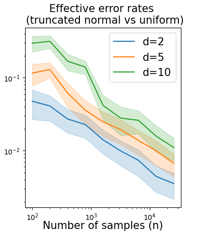
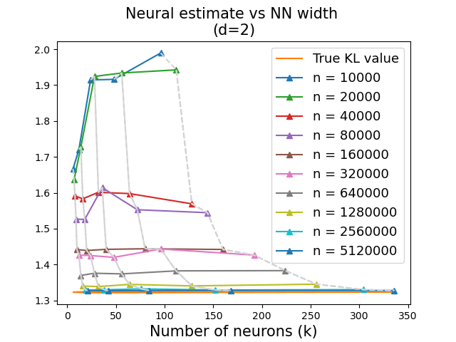
Fig. 1: Neural estimate of KL divergence: (a) estimate versus nn convergence in dimension d=2d=2, for PP given by 𝒩⁡(𝟎,I2)\mathcal{N}(\mathbf{0},\mathrm{I}_{2}) truncated to be supported inside 𝒳=[0.1,2]×[−1,0]\mathcal{X}=[0.1,2]\times[-1,0] and Q=𝖴𝗇𝗂𝖿⁡(𝒳)Q=\mathsf{Unif}(\mathcal{X}); (b) estimate versus nn convergence in dimension d=5d=5, for PP given by 𝒩⁡(𝟎,I5)\mathcal{N}(\mathbf{0},\mathrm{I}_{5}) truncated to 𝒳=[0.1,2]×[−1,0]×[2,3]×[−2,−1.5]×[−1,1]\mathcal{X}=[0.1,2]\times[-1,0]\times[2,3]\times[-2,-1.5]\times[-1,1] and Q=𝖴𝗇𝗂𝖿⁡(𝒳)Q=\mathsf{Unif}(\mathcal{X}); (c) similar to (b) but in dimension d=10d=10 and with compact support 𝒳×𝒳\mathcal{X}\times\mathcal{X}; (d) effective error rates versus number of samples; (e) estimate versus number of neurons kk, for fixed number of samples nn.

Let H^𝒢~k​(𝐚k,t)2​(Xn,Yn):=𝖧^γH2,𝒢~k​(𝐚k,t)​(Xn,Yn)\hat{H}^{2}_{\tilde{\mathcal{G}}_{k}(\mathbf{a}_{k},t)}(X^{n},Y^{n}):=\hat{\mathsf{H}}_{\gamma_{H^{2}},\tilde{\mathcal{G}}_{k}(\mathbf{a}_{k},t)}(X^{n},Y^{n}), where t>0t>0 and 𝒢~k​(𝐚,t)\tilde{\mathcal{G}}_{k}(\mathbf{a},t) is the NN class

𝒢~k(𝐚,t):={g:ℝd→ℝ:g⁡(x)=(1−t)∧g~​(x),g~∈𝒢k​(𝐚)}.\mspace{-10mu}\tilde{\mathcal{G}}_{k}\mspace{-3mu}\left(\mathbf{a},t\right)\mspace{-3mu}:=\mspace{-3mu}\left\{\mspace{-3mu}g:\mathbb{R}^{d}\mspace{-3mu}\rightarrow\mathbb{R}:\begin{aligned} &g(x)\mspace{-3mu}=\mspace{-3mu}(1-t)\wedge\tilde{g}(x),\\ &\tilde{g}\in\mathcal{G}_{k}(\mathbf{a})\end{aligned}\right\}. (30)

Set

ℐH2(m):={f:𝒳→ℝ,cB⋆​(f)∨‖(1−f)−1‖∞∨‖f‖∞≤m},\mathcal{I}_{H^{2}}(m):=\mspace{-3mu}\left\{f:\mathcal{X}\rightarrow\mathbb{R},\begin{aligned} &c_{B}^{\star}(f)\vee\mspace{-3mu}\left\|(1-f)^{-1}\right\|_{\infty}\mspace{-5mu}\\ &\vee\left\|f\right\|_{\infty}\mspace{-5mu}\leq m\end{aligned}\right\},

and 𝒫H2​(𝒳)\mathcal{P}_{H^{2}}(\mathcal{X}) as the collection of all (P,Q)∈𝒫⁡(𝒳)×𝒫⁡(𝒳)(P,Q)\in\mathcal{P}(\mathcal{X})\times\mathcal{P}(\mathcal{X}) such that P≪QP\ll Q (note that 0≤H2​(P,Q)≤20\leq H^{2}(P,Q)\leq 2). Define the shorthands 𝒢~k,t(1)=𝒢~k​(𝟏,t)\tilde{\mathcal{G}}_{k,t}^{(1)}=\tilde{\mathcal{G}}_{k}(\mathbf{1},t),

𝒢~k,m,t(2):=𝒢~k​(k​log⁡k,2​k−1​m,m,t).\tilde{\mathcal{G}}_{k,m,t}^{(2)}:=\tilde{\mathcal{G}}_{k}\left(\sqrt{k}\log k,2k^{-1}m,m,t\right).

The next theorem establishes consistency of the NE and bounds its effective absolute-error (see Appendix D-A for proof).

Theorem 6 (H2H^{2} neural estimation).

Let (P,Q)∈𝒫H2​(𝒳)(P,Q)\in\mathcal{P}_{H^{2}}(\mathcal{X}). For any α>0:\alpha>0:

  1. (i)

    If fH2∈𝖢⁡(𝒳)f_{H^{2}}\in\mathsf{C}\left(\mathcal{X}\right), then, for {kn,tkn}n∈ℕ\{k_{n},t_{k_{n}}\}_{n\in\mathbb{N}}, such that kn→∞k_{n}\rightarrow\infty, tkn>0,tkn→0t_{k_{n}}>0,~t_{k_{n}}\rightarrow 0, and kn32​tkn−2=O⁡(n(1−α)/2)k_{n}^{\frac{3}{2}}t_{k_{n}}^{-2}=O\left(n^{(1-\alpha)/2}\right),

    H^𝒢~kn,tkn(1)2​(Xn,Yn)→n→∞H2​(P,Q),ℙ−a.s.\displaystyle\mspace{-10mu}\hat{H}^{2}_{\tilde{\mathcal{G}}_{k_{n},t_{k_{n}}}^{(1)}}\mspace{-4mu}(X^{n},Y^{n})\xrightarrow[n\rightarrow\infty]{}H^{2}(P,Q),\quad\mathbb{P}-\mbox{a.s.} (31)
  2. (ii)

    Suppose there exists MM such that fH2∈ℐH2​(M)f_{H^{2}}\in\mathcal{I}_{H^{2}}(M). Then, for k,nk,n with log3⁡k​k=O⁡(n(1−α)/2)\log^{3}k\sqrt{k}=O\left(n^{(1-\alpha)/2}\right), mk=0.5​log⁡km_{k}=0.5\log k and tk=log−1⁡kt_{k}=\log^{-1}k, we have

    𝔼⁡[|H^𝒢~k,mk,tk(2)2​(Xn,Yn)−H2​(P,Q)|]\displaystyle\mathbb{E}\left[\left|\hat{H}^{2}_{\tilde{\mathcal{G}}_{k,m_{k},t_{k}}^{(2)}}(X^{n},Y^{n})-H^{2}(P,Q)\right|\right]
    =(log⁡k​k−12)+O⁡(log3⁡k​k​n−12).\displaystyle\qquad\quad=\left(\log k~k^{-\frac{1}{2}}\mspace{-2.5mu}\right)+O\left(\log^{3}k\sqrt{k}~n^{\mspace{-2mu}-\frac{1}{2}}\mspace{-2mu}\right). (32)

To establish effective error bounds for squared Hellinger distance, we used a truncated NN class 𝒢~k​(𝐚,t)\tilde{\mathcal{G}}_{k}\mspace{-3mu}\left(\mathbf{a},t\right) given in (30), which is the function class obtained by saturating the shallow NN output to 1−t1-t for some t>0t>0. This is done since γH2​(x)\gamma_{H^{2}}(x) has a singularity at x=1x=1 and the NN outputs must be truncated below 1 so as to satisfy (16) for bounding the empirical estimation error. For obtaining effective error bounds under this constraint, we scale the parameter tt with kk as {tk}k∈ℕ\{t_{k}\}_{k\in\mathbb{N}} for some decreasing positive sequence tk→0t_{k}\rightarrow 0. The bound in (32) uses tk=log−1⁡kt_{k}=\log^{-1}k.

Remark 9 (Effective sample complexity).

In Appendix D-A, we obtain effective error bounds (see (119)) for an arbitrary decreasing positive sequence {tk}k∈ℕ\{t_{k}\}_{k\in\mathbb{N}}, with tk→0t_{k}\rightarrow 0, and an increasing positive divergent sequence {mk}k∈ℕ\{m_{k}\}_{k\in\mathbb{N}}. If fH2∈ℐH2​(M)f_{H^{2}}\in\mathcal{I}_{H^{2}}(M) and the NN parameters can depend on MM, then, for kk, tk=log−1⁡kt_{k}=\log^{-1}k and nn such that k​log2​k=O⁡(n(1−α)/2)\sqrt{k}\log^{2}k=O\left(n^{(1-\alpha)/2}\right), setting mk=Mm_{k}=M in (119) yields

𝔼⁡[|H^𝒢~k,M,tk(2)2​(Xn,Yn)−H2​(P,Q)|]\displaystyle\mathbb{E}\left[\left|\hat{H}^{2}_{\tilde{\mathcal{G}}_{k,M,t_{k}}^{(2)}}(X^{n},Y^{n})-H^{2}(P,Q)\right|\right]
=O⁡(k−12​log⁡k)+O⁡(k​log2​k​n−12).\displaystyle\qquad\quad\ =O\mspace{-4mu}\left(\mspace{-2mu}k^{-\frac{1}{2}}\log k\mspace{-2.5mu}\right)+\mspace{-3mu}O\mspace{-3mu}\left(\sqrt{k}~\log^{2}kn^{-\frac{1}{2}}\mspace{-3mu}\right). (33)

The optimal choice of kk in (33) is k=n12​(1+η)k=n^{\frac{1}{2(1+\eta)}}, (\big(for 𝑂𝑃𝐸𝑁α<0.5​(1−2​η)​(1+η)−1)\alpha<0.5(1-2\eta)(1+\eta)^{-1}\big), where η>0\eta>0 is an arbitrarily small. The resulting effective error bound is O(n−1/4)O(n^{-1/4}).

IV Empirical Results

We illustrate the performance of KL divergence neural estimation via some simple simulations. The considered NN class is 𝒢k∗​(M)\mathcal{G}_{k}^{*}(M) (see Section III-D) with MM appropriately chosen. The number of samples nn varies from n=105n=10^{5} to n=6.4×10⁶n=6.4\times 10^{6}, and we scale the NN size as k=n1/5k=n^{1/5} (in accordance with k=O⁡(n1−α)k=O\left(n^{1-\alpha}\right) for α>0\alpha>0 sufficiently small, see (22)). The NN is trained using Adam optimizer (Kingma and Ba 2017) for 200 epochs. The initial learning rate of 10−210^{-2} is reduced to 10−310^{-3} after the first 100 epochs. We use batch size n×10−3n\times 10^{-3}, and present plots averaged over 10 different runs (shown as dots in Figures 1(a)-1(c)).

Figure 1(a) shows convergence of the NE of 𝖣𝖪𝖫​(P∥Q)\mathsf{D}_{\mathsf{KL}}\left(P\middle\|Q\right) versus number of samples, when PP is a 2-dimensional truncated Gaussians (adhering to the compact support assumption) and QQ is uniform distribution on the same support. For Figure 1(a), we start from P~=𝒩⁡(𝟎,I2)\tilde{P}=\mathcal{N}(\mathbf{0},\mathrm{I}_{2}), where Id∈ℝd×d\mathrm{I}_{d}\in\mathbb{R}^{d\times d} is the identity, and truncate (and normalize) it to 𝒳=[0.1,2]×[−1,0]\mathcal{X}=[0.1,2]\times[-1,0] to obtain PP, and set Q=𝖴𝗇𝗂𝖿⁡(𝒳)Q=\mathsf{Unif}(\mathcal{X}). Figure 1(b) repeats the experiment but with PP as a 5-dimensional Gaussian 𝒩⁡(𝟎,I5)\mathcal{N}(\mathbf{0},\mathrm{I}_{5}) truncated to 𝒳:=[0.1,2]×[−1,0]×[2,3]×[−2,−1.5]×[−1,1]\mathcal{X}:=[0.1,2]\times[-1,0]\times[2,3]\times[-2,-1.5]\times[-1,1] and Q=𝖴𝗇𝗂𝖿⁡(𝒳)Q=\mathsf{Unif}(\mathcal{X}). The same setup but in dimension d=10d=10 and with 𝒳×𝒳\mathcal{X}\times\mathcal{X} (instead of 𝒳\mathcal{X}) is presented in Figure 1(c) (blue curve). Corresponding error rates (for effective error averaged over 100 runs) versus number of samples (on a log-log scale) are shown in Figure 1(d). It can be seen therein that the convergence rate is parametric for large enough values of nn.

While convergence is evident in all dimensions, the trajectories are different: convergence happens from above when dd is small and from below for large dd (with d=5d=5 sitting in between and presenting a mixed trend). This happens because the same NN size k=n1/5k=n^{1/5} were used in all three experiments, without factoring in the dimension (generally, higher-dimensional distribution need a larger NN). This results in the NN being relatively large when d=2d=2, which causes overfitting and, in turn, overestimation of the KL divergence for small nn values. For d=10d=10, that same NN is relatively small, resulting in underestimation for small nn. In accordance with the above, the d=5d=5 case exhibits a mixed trend. To verify this effect, we increased the NN size by a factor of 5 in the d=10d=10 experiment—the obtained neural estimator is shown by the red curve in Figure 1(c). As expected, the larger networks results in convergence from above, similarly to the original d=2d=2 example.

To further examine the overfitting effect, Figure 1(e) revisits the setup of Figure 1(a) and shows the evolution of the neural estimate as the number of neurons kk grows, keeping nn fixed. The neural estimate progressively gets closer to the true value as nn becomes larger. The overestimation of the KL divergence again highlights overfitting. The increase in the KL divergence estimate with kk could also be due to higher optimization error for larger kk values. The light gray lines across curves for different nn values show convergence to true 𝖣𝖪𝖫​(P∥Q)\mathsf{D}_{\mathsf{KL}}\left(P\middle\|Q\right).

V Concluding Remarks

This paper studied neural estimation of SDs, aiming to characterize tradeoffs between approximation and empirical estimation errors. We showed that NEs of 𝖿\mathsf{f}-divergences, such as the KL and χ2\chi^{2} divergences and the squared Hellinger distance, are consistent, provided the appropriate scaling of the NN size kk with the sample size nn. We then derived non-asymptotic absolute-error upper bounds that quantify the desired tradeoff between kk and nn. The key technical results leading to these bounds are Theorems 2-3, which, respectively, bound the sup-norm approximation error by NNs and the empirical estimation error of the parametrized SD.

Going forward, we aim to extend our results to additional SDs such as the total variation distance, the 11-Wasserstein distance, etc. While the high level analysis extends to these examples, new approximation bounds for the appropriate function classes (bounded or 1-Lipschitz) are needed. Another extension of interest is to PP and QQ that are not compactly supported. This is possible within our framework under proper tail decay, but we leave the details for future work. While we have neglected the optimization error from our current analysis, this is an important component of the overall estimation error and we plan to examine it in the future. Lastly, generalizing our analysis to NEs based on deep neural networks is another important extension. Through the results herein and the said future directions, we hope to provide useful performance guarantees for NEs that would facilitate a principled usage thereof in ML applications and beyond.

References

  • Ali and Silvey (1966) S. M. Ali and S. D. Silvey. A general class of coefficients of divergence of one distribution from another. Journal of the Royal Statistical Society: Series B (Methodological), 28(1):131–142, Jan. 1966.
  • Arjovsky et al. (2017) M. Arjovsky, S. Chintala, and L. Bottou. Wasserstein generative adversarial networks. In Proceedings of the International Conference on Machine Learning (ICML-2017), pages 214–223, Sydney, Australia, Jul. 2017.
  • Arora et al. (2017) S. Arora, R. Ge, Y. Liang, T. Ma, and Y. Zhang. Generalization and equilibrium in generative adversarial nets (GANs). In Proceedings of the International Conference on Machine Learning (ICML-2017), pages 224–232, Sydney, Australia, Jul. 2017.
  • Barron (1992) A. R. Barron. Neural net approximation. Proceedings of Seventh Yale Workshop on Adaptive and Learning Systems, CT, USA, 20–22 May 1992.
  • Barron (1993) A. R. Barron. Universal approximation bounds for superpositions of a sigmoidal function. IEEE Transactions on Information Theory, 39(3):930–945, 1993.
  • Barron (1994) A. R. Barron. Approximation and estimation bounds for artificial neural networks. Mach. Learn., 14(1):115–133, Jan. 1994.
  • Belghazi et al. (2018) M. I. Belghazi, A. Baratin, S. Rajeshwar, S. Ozair, Y. Bengio, A. Courville, and D. Hjelm. Mutual information neural estimation. In Proceedings of the 35th International Conference on Machine Learning, volume 80, pages 531–540, Stockholm Sweden, 10–15 Jul 2018.
  • Berrett et al. (2019) T. B. Berrett, R. J. Samworth, and M. Yuan. Efficient multivariate entropy estimation via kk-nearest neighbour distances. The Annals of Statistics, 47(1):288–318, 2019.
  • Csiszár (1967) I. Csiszár. Information-type measures of difference of probability distributions and indirect observation. Studia Ccientiarum Mathematicarum Hungarica, 2:229–318, 1967.
  • Dognin et al. (2019) P. Dognin, I. Melnyk, Y. Mroueh, J. Ross, C. D. Santos, and T. Sercu. Wasserstein barycenter model ensembling. In Proceedings of the International Conference on Learning Representations (ICLR-2019), New Orleans, Louisiana, US, May 2019.
  • Goodfellow et al. (2014) I. Goodfellow, J. Pouget-Abadie, M. Mirza, B. Xu, D. Warde-Farley, S. Ozair, A. Courville, and Y. Bengio. Generative adversarial nets. In Proceedings of the Annual Conference on Advances in Neural Information Processing Systems (NeurIPS-2014), pages 2672–2680, 2014.
  • Gramfort et al. (2015) A. Gramfort, G. Peyré, and M. Cuturi. Fast optimal transport averaging of neuroimaging data. In Proceedings of the International Conference on Information Processing in Medical Imaging, pages 261–272, Hong Kong, China, Jun. 2015.
  • Han et al. (2020) Y. Han, J. Jiao, T. Weissman, and Y. Wu. Optimal rates of entropy estimation over Lipschitz balls. The Annals of Statistics, 48(6):3228 – 3250, 2020.
  • Kandasamy et al. (2015) K. Kandasamy, A. Krishnamurthy, B. Poczos, L. Wasserman, and J. M. Robins. Nonparametric von Mises estimators for entropies, divergences and mutual informations. In Proceedings of the Annual Conference on Advances in Neural Information Processing Systems (NeurIPS-2015), pages 397–405, Montréal, Canada, 2015.
  • Kingma and Ba (2017) D. P. Kingma and J. Ba. Adam: A method for stochastic optimization. arXiv preprint arXiv:1412.6980, 2017.
  • Kingma and Welling (2014) D. P. Kingma and M. Welling. Auto-encoding variational bayes. In Proceedings of the International Conference on Learning Representations (ICLR-2014), Banff, Canada, Apr. 2014.
  • Krishnamurthy et al. (2014) A. Krishnamurthy, K. Kandasamy, B. Póczos, and L. Wasserman. Nonparametric estimation of Rényi divergence and friends. In Proceedings of the International Conference on Machine Learning (ICML-2014), pages 919–927, Beijing, China, Jun. 2014.
  • Liang (2019) T. Liang. Estimating certain Integral Probability Metric (IPM) is as hard as estimating under the IPM. arXiv preprint arXiv:1911.00730, Nov. 2019.
  • Lu et al. (2017) Z. Lu, H. Pu, F. Wang, Z. Hu, and L. Wang. The expressive power of neural networks: A view from the width. In Proceedings of the Annual Conference on Advances in Neural Information Processing Systems (NeurIPS-2017), pages 6231–6239, Long Beach, CA, US, Dec. 2017.
  • Müller (1997) A. Müller. Integral probability metrics and their generating classes of functions. Advances in Applied Probability, 29(2):429–443, 1997.
  • Nguyen et al. (2010) X. Nguyen, M. J. Wainwright, and M. I. Jordan. Estimating divergence functionals and the likelihood ratio by convex risk minimization. IEEE Transactions on Information Theory, 56(11):5847–5861, 2010.
  • Nowozin et al. (2016) S. Nowozin, B. Cseke, and R. Tomioka. ff-GAN: Training generative neural samplers using variational divergence minimization. In Proceedings of the Annual Conference on Advances in Neural Information Processing Systems (NeurIPS-2016), pages 271–279, Barcelona, Spain, Dec. 2016.
  • Perez-Cruz (2008) F. Perez-Cruz. Kullback-leibler divergence estimation of continuous distributions. In 2008 IEEE International Symposium on Information Theory, pages 1666–1670, 2008.
  • Póczos et al. (2011) B. Póczos, L. Xiong, and J. Schneider. Nonparametric divergence estimation with applications to machine learning on distributions. In Proceedings of the Twenty-Seventh Conference on Uncertainty in Artificial Intelligence, page 599–608. AUAI Press, 2011.
  • Rabin et al. (2011) J. Rabin, G. Peyré, J. Delon, and M. Bernot. Wasserstein barycenter and its application to texture mixing. In Proceedings of the International Conference on Scale Space and Variational Methods in Computer Vision (SSVM-2011), pages 435–446, Gedi, Israel, May 2011.
  • Stinchcombe and White (1990) M. Stinchcombe and H. White. Approximating and learning unknown mappings using multilayer feedforward networks with bounded weights. In Proceedings of the International Joint Conference on Neural Networks (IJCNN-1990), pages 7–16, San Diego, CA, US, Jun. 1990.
  • Tolstikhin et al. (2018) I. Tolstikhin, O. Bousquet, S. Gelly, and B. Schölkopf. Wasserstein auto-encoders. In International Conference on Learning Representations (ICLR-2018), Vancouver, Canada, Apr.-May 2018.
  • Van Der Vaart and Wellner (1996) A. Van Der Vaart and J. A. Wellner. Weak Convergence and Empirical Processes. Springer, New York, 1996.
  • van Handel (2016) R. van Handel. Probability in High Dimension: Lecture Notes-Princeton University. [Online]. Available: https://web.math.princeton.edu/~rvan/APC550.pdf, 2016.
  • Villani (2008) C. Villani. Optimal Transport: Old and New, volume 338. Springer Science & Business Media, 2008.
  • Wang et al. (2005) Q. Wang, S. R. Kulkarni, and S. Verdu. Divergence estimation of continuous distributions based on data-dependent partitions. IEEE Transactions on Information Theory, 51(9):3064–3074, 2005.
  • Yukich et al. (1995) J. E. Yukich, M. B. Stinchcombe, and H. White. Sup-norm approximation bounds for networks through probabilistic methods. IEEE Transactions on Information Theory, 41(4):1021–1027, 1995.
  • Zhang et al. (2018) P. Zhang, Q. Liu, D. Zhou, T. Xu, and X. He. On the discrimination-generalization tradeoff in GANs. In Proceedings of the International Conference on Learning Representations (ICLR-2018), Vancouver, Canada, Apr.-May 2018.
  • Zolotarev (1983) V. M. Zolotarev. Probability metrics. Teoriya Veroyatnostei i ee Primeneniya, 28(2):264–287, 1983.

Appendix A Appendix

To emphasize the underlying parameters of the NN, by some abuse of notation, we introduce

𝒢k(Θ):={g:ℝd→ℝ:g⁡(x)=∑i=1kβi​ϕ​(wi⋅x+bi)+b0,({βi,wi,bi}i=1k,b0)∈Θ},\mathcal{G}_{k}(\Theta):=\mspace{-3mu}\left\{g:\mathbb{R}^{d}\mspace{-5mu}\rightarrow\mathbb{R}:\begin{aligned} &g(x)=\sum_{i=1}^{k}\beta_{i}\phi\left(w_{i}\cdot x+b_{i}\right)+b_{0},~\mspace{-3mu}\big(\{\beta_{i},w_{i},b_{i}\}_{i=1}^{k},b_{0}\big)\in\Theta\end{aligned}\mspace{-10mu}\right\}, (34a)
Θk(𝐚):={({βi,wi,bi}i=1k,b0):wi∈ℝd,b0,bi,βi∈ℝ,maxi=1,…,kj=1,…,d⁡{|wi,j|,|bi|}≤a1|βi|≤a2,i=1,…,k,|b0|≤a3}.\Theta_{k}(\mathbf{a}):=\left\{\left(\{\beta_{i},w_{i},b_{i}\}_{i=1}^{k},b_{0}\right):\ \ \begin{aligned} &w_{i}\in\mathbb{R}^{d},~b_{0},b_{i},\beta_{i}\in\mathbb{R},~\max\nolimits_{\begin{subarray}{c}i=1,\ldots,k\\ j=1,\ldots,d\end{subarray}}\left\{|w_{i,j}|,|b_{i}|\right\}\leq a_{1}\\ &|\beta_{i}|\leq a_{2},~~i=1,\ldots,k,~|b_{0}|\leq a_{3}\end{aligned}\right\}. (34b)

Also, throughout the Appendix, we denote g⁡(x)=∑i=1kβi​ϕ​(wi⋅x+bi)+b0g(x)=\sum_{i=1}^{k}\beta_{i}\phi\left(w_{i}\mspace{-3mu}\cdot\mspace{-3mu}x\mspace{-2mu}+\mspace{-2mu}b_{i}\right)\mspace{-2mu}+\mspace{-2mu}b_{0} for θ=({βi,wi,bi}i=1k,b0)\theta=\big(\{\beta_{i},w_{i},b_{i}\}_{i=1}^{k},b_{0}\big) by gθg_{\theta}, whenever the underlying θ\theta needs to be emphasized.

We first state an auxiliary result which will be useful in the proofs that follow. For b≥0b\geq 0, an integer l≥0l\geq 0, and an open set 𝒰⊆ℝd\mathcal{U}\subseteq\mathbb{R}^{d} containing the origin, consider the class 𝒮l,b​(𝒰)\mathcal{S}_{l,b}(\mathcal{U}) of square-integrable functions defined below:

𝒮l,b(𝒰):={f∈L1(𝒰)∪L2(𝒰):|f⁡(0)|≤b,D𝜶​f​ exists Lebesgue a.e. on ​𝒰​∀𝜶​ s.t. |𝜶|=l,‖D𝜶​f‖L2​(𝒰)≤b​ for ​|𝜶|∈{1,l}}.\mathcal{S}_{l,b}(\mathcal{U}):=\left\{f\in L^{1}(\mathcal{U})\cup L^{2}(\mathcal{U}):\ \ \begin{aligned} &\left|f(0)\right|\leq b,~D^{\bm{\alpha}}f\mbox{ exists Lebesgue a.e. on }\mathcal{U}~\forall\bm{\alpha}\mbox{ s.t. }|\bm{\alpha}|=l,\\ &\left\|D^{\bm{\alpha}}f\right\|_{L^{2}(\mathcal{U})}\leq b\mbox{ for }\left|\bm{\alpha}\right|\in\{1,l\}\end{aligned}\right\}. (35)

The following lemma states that functions in 𝒮l,b​(ℝd)\mathcal{S}_{l,b}(\mathbb{R}^{d}) with sufficient smoothness order ll belong to the Barron class. Its proof essentially follows using arguments from Barron 1993, where it was mentioned without explicit quantification. Below, we provide a proof for completeness.

Lemma 1 (Smoothness and Barron class).

If f∈𝒮s,b​(ℝd)f\in\mathcal{S}_{s,b}\left(\mathbb{R}^{d}\right) for s:=⌊d2⌋+2s:=\lfloor\frac{d}{2}\rfloor+2, then we have

B⁡(f)≤b​κd​d,\displaystyle B(f)\leq b\kappa_{d}~\sqrt{d}, (36a)
κd2:=(d+ds)​∫ℝd(1+‖ω‖2​(s−1))−1​𝑑ω<∞.\displaystyle\kappa_{d}^{2}:=(d+d^{s})\int_{\mathbb{R}^{d}}\big(1+\left\|\omega\right\|^{2(s-1)}\big)^{\mspace{-3mu}-1}\,\mathsf{d}\omega<\infty. (36b)

Consequently, 𝒮s,b​(ℝd)⊆ℬb​κd​d∨b\mathcal{S}_{s,b}\left(\mathbb{R}^{d}\right)\subseteq\mathcal{B}_{b\kappa_{d}\sqrt{d}\vee b}.

Proof.

Since f∈L1​(ℝd)∪L2​(ℝd)f\in L^{1}\left(\mathbb{R}^{d}\right)\cup L^{2}\left(\mathbb{R}^{d}\right), its Fourier transform f^​(ω)\hat{f}(\omega) exists, and hence, F⁡(d​ω)=|f^​(ω)|​d​ωF(d\omega)=\left|\hat{f}(\omega)\right|d\omega. Then, it follows that

B⁡(f)=∫ℝdsupx∈𝒳|ω⋅x|​|f^​(ω)|​𝑑ω≤d​∫ℝd‖ω‖​|f^​(ω)|​𝑑ω,\displaystyle B(f)=\int_{\mathbb{R}^{d}}\sup_{x\in\mathcal{X}}\left|\omega\cdot x\right|\left|\hat{f}(\omega)\right|d\omega\leq\sqrt{d}\int_{\mathbb{R}^{d}}\left\|\omega\right\|\left|\hat{f}(\omega)\right|d\omega, (37)

where we used supx∈𝒳|ω⋅x|≤d​‖ω‖\sup_{x\in\mathcal{X}}\left|\omega\cdot x\right|\leq\sqrt{d}\left\|\omega\right\| which holds by Cauchy-Schwarz inequality.

Next, recall that if the partial derivatives D𝜶​fD^{\bm{\alpha}}f, |𝜶|=s|\bm{\alpha}|=s, exists on ℝd\mathbb{R}^{d}, then all partial derivatives D𝜶​fD^{\bm{\alpha}}f, 0≤|𝜶|≤s0\leq|\bm{\alpha}|\leq s, also exists. Hence, if ‖D𝜶​f‖L2​(ℝd)≤b\left\|D^{\bm{\alpha}}f\right\|_{L^{2}\left(\mathbb{R}^{d}\right)}\leq b for all α\alpha with |α|∈{1,s}\left|\alpha\right|\in\{1,s\}, we have

∫ℝd‖ω‖​|f^​(ω)|​𝑑ω\displaystyle\int_{\mathbb{R}^{d}}\left\|\omega\right\|\left|\hat{f}(\omega)\right|d\omega ≤(a)(∫ℝdd​ω1+‖ω‖2​(s−1))12​(∫ℝd(‖ω‖2+‖ω‖2​s)​|f^​(ω)|2​𝑑ω)12\displaystyle\stackrel{{\scriptstyle(a)}}{{\leq}}\left(\int_{\mathbb{R}^{d}}\frac{d\omega}{1+\left\|\omega\right\|^{2(s-1)}}\right)^{\frac{1}{2}}\left(\int_{\mathbb{R}^{d}}\left(\left\|\omega\right\|^{2}+\left\|\omega\right\|^{2s}\right)\left|\hat{f}(\omega)\right|^{2}d\omega\right)^{\frac{1}{2}} (38)
≤(b)(∫ℝdd​ω1+‖ω‖2​(s−1))12(∑𝜶:|𝜶|=1‖D𝜶f‖L2​(ℝd)2+∑𝜶:|𝜶|=s‖D𝜶f‖L2​(ℝd)2)12\displaystyle\stackrel{{\scriptstyle(b)}}{{\leq}}\left(\int_{\mathbb{R}^{d}}\frac{d\omega}{1+\left\|\omega\right\|^{2(s-1)}}\right)^{\frac{1}{2}}\left(\sum_{\bm{\alpha}:\left|\bm{\alpha}\right|=1}\left\|D^{\bm{\alpha}}f\right\|^{2}_{L^{2}\left(\mathbb{R}^{d}\right)}+\sum_{\bm{\alpha}:\left|\bm{\alpha}\right|=s}\left\|D^{\bm{\alpha}}f\right\|^{2}_{L^{2}\left(\mathbb{R}^{d}\right)}\right)^{\frac{1}{2}}
≤(c)κd​b,\displaystyle\stackrel{{\scriptstyle(c)}}{{\leq}}\kappa_{d}b, (39)

where

  1. (a)

    follows from Cauchy-Schwarz inequality;

  2. (b)

    is due to Plancherel’s theorem;

  3. (c)

    follows since |{𝜶:|𝜶|=s}|=ds\left|\{\bm{\alpha}:\left|\bm{\alpha}\right|=s\}\right|=d^{s} and ‖D𝜶​f‖L2​(ℝd)≤b\left\|D^{\bm{\alpha}}f\right\|_{L^{2}\left(\mathbb{R}^{d}\right)}\leq b.

Combining (37) and (39) leads to (36a). The final claim follows from (5) and (36a) by noting that |f⁡(0)|≤b\left|f(0)\right|\leq b by definition. ∎

A-A Proof of Theorem 2

The proof relies on arguments from Barron 1992 and Barron 1993, along with the uniform central limit theorem for uniformly bounded VC function classes. Fix an arbitrary (small) δ>0\delta>0, and let f:ℝd→ℝf:\mathbb{R}^{d}\rightarrow\mathbb{R} be such that f~=f|𝒳\tilde{f}=f|_{\mathcal{X}} and B⁡(f)∨f⁡(0)≤c+δB(f)\vee f(0)\leq c+\delta. This is possible since cB⋆​(f~)≤cc_{B}^{\star}(\tilde{f})\leq c. Then, it follows from the proof of Barron 1993 that

f0​(x):=f⁡(x)−f⁡(0)=∫ω∈ℝd∖{0}ϱ⁡(x,ω)​μ​(𝑑ω),\displaystyle f_{0}(x):=f(x)-f(0)=\int_{\omega\in\mathbb{R}^{d}\setminus\{0\}}\varrho(x,\omega)\mu(d\omega),

where

ϱ⁡(x,ω)=B⁡(f)supx∈𝒳|ω⋅x|​(cos⁡(ω⋅x+ζ⁡(ω))−cos⁡(ζ⁡(ω))),\displaystyle\varrho(x,\omega)=\frac{B(f)}{\sup_{x\in\mathcal{X}}\left|\omega\cdot x\right|}\left(\cos(\omega\cdot x+\zeta(\omega))-\cos(\zeta(\omega))\right),
B⁡(f):=∫ℝdsupx∈𝒳|ω⋅x|​F​(𝑑ω),\displaystyle B(f):=\int_{\mathbb{R}^{d}}\sup_{x\in\mathcal{X}}\left|\omega\cdot x\right|F(d\omega),
μ⁡(d​ω)=supx∈𝒳|ω⋅x|​F​(d​ω)B⁡(f),\displaystyle\mu(d\omega)=\frac{\sup_{x\in\mathcal{X}}\left|\omega\cdot x\right|F(d\omega)}{B(f)},

and ζ:ℝd→ℝ\zeta:\mathbb{R}^{d}\rightarrow\mathbb{R}. Note that μ∈𝒫⁡(ℝd)\mu\in\mathcal{P}(\mathbb{R}^{d}) is a probability measure.

Let Θ~1​(k,B⁡(f)):=Θ1​(k​log⁡k,2​B​(f),0)\tilde{\Theta}_{1}\left(k,B(f)\right):=\Theta_{1}(\sqrt{k}\log k,2B(f),0) (see (34b)). Then, it further follows from the proofs44 4 The claims in Barron 1993 are stated for L2L_{2} norm, but it is not hard to see from the proof therein that the same also holds for L∞L^{\infty} norm, apart from the following subtlety. In the proof of Lemma 3, it is shown that ϱ⁡(x,ω)\varrho(x,\omega), ω∈ℝd\omega\in\mathbb{R}^{d}, lies in the convex closure of a certain class of step functions, whose discontinuity points are adjusted to coincide with the continuity points of the underlying measure μ\mu. Similarly, here, the step discontinuities needs to be adjusted to coincide with the continuity points of both PP and QQ. Nevertheless, the same arguments hold since the common continuity points of PP and QQ form a dense set. of Barron 1993 that there exists a probability measure μk∈𝒫⁡(Θ~1​(k,B⁡(f)))\mu_{k}\in\mathcal{P}\left(\tilde{\Theta}_{1}\left(k,B(f)\right)\right) (see Barron 1993) such that

‖f0−∫θ∈Θ~1​(k,B⁡(f))gθ​(⋅)​μk​(𝑑θ)‖∞,P,Q≤2​(B​(f)+1)k,\displaystyle\left\|f_{0}-\int_{\theta\in\tilde{\Theta}_{1}\left(k,B(f)\right)}g_{\theta}(\cdot)~\mu_{k}\left(d\theta\right)\right\|_{\infty,P,Q}\leq\frac{2(B(f)+1)}{\sqrt{k}}, (40)

where gθ​(x)=β​ϕ​(w⋅x+b)g_{\theta}(x)=\beta\phi\left(w\cdot x+b\right) for θ=(β,w,b)\theta=(\beta,w,b). Note that ∫Θ~1​(k,B​(f))μk​(𝑑θ)=1<∞\int_{\tilde{\Theta}_{1}\left(k,B(f)\right)}\mu_{k}(d\theta)=1<\infty.

Next, for each fixed xx, let υx:Θ~1​(k,B⁡(f))→ℝ\upsilon_{x}:\tilde{\Theta}_{1}\left(k,B(f)\right)\rightarrow\mathbb{R} be given by υx​(θ):=gθ​(x)\upsilon_{x}(\theta):=g_{\theta}(x), and consider the function class 𝒱k​(Θ~1​(k,B⁡(f)))={υx,x∈ℝd}\mathcal{V}_{k}\left(\tilde{\Theta}_{1}\left(k,B(f)\right)\right)=\left\{\upsilon_{x},~x\in\mathbb{R}^{d}\right\}. Note that every υx∈𝒱k​(Θ~1​(k,B⁡(f)))\upsilon_{x}\in\mathcal{V}_{k}\left(\tilde{\Theta}_{1}\left(k,B(f)\right)\right) is a composition of an affine function in θ\theta with the bounded monotonic function β​ϕ​(⋅)\beta\phi(\cdot). Hence, noting that 𝒱k​(Θ~1​(k,B⁡(f)))\mathcal{V}_{k}\left(\tilde{\Theta}_{1}\left(k,B(f)\right)\right) is a VC function class (Van Der Vaart and Wellner 1996), it follows from Van Der Vaart and Wellner 1996 that it is a uniform Donsker class (in particular, μk\mu_{k}-Donsker) for all probability measures μ∈𝒫⁡(Θ~1​(k,B⁡(f)))\mu\in\mathcal{P}\left(\tilde{\Theta}_{1}\left(k,B(f)\right)\right). Furthermore, an application of Van Der Vaart and Wellner 1996) yields that there exists kk parameter vectors, θi:=(βi,wi,bi)∈Θ~1​(k,B⁡(f)),1≤i≤k\theta_{i}:=(\beta_{i},w_{i},b_{i})\in\tilde{\Theta}_{1}\left(k,B(f)\right),~1\leq i\leq k, such that (see also Yukich et al. 1995)

supx∈ℝd|∫θ∈Θ~1​(k,B⁡(f))gθ​(x)​μk​(𝑑θ)−1k​∑i=1kgθi​(x)|≤c^d​B​(f)​k−12,\displaystyle\sup_{x\in\mathbb{R}^{d}}\left|\int_{\theta\in\tilde{\Theta}_{1}\left(k,B(f)\right)}g_{\theta}(x)~\mu_{k}(d\theta)-\frac{1}{k}\sum_{i=1}^{k}g_{\theta_{i}}(x)\right|\leq\hat{c}_{d}B(f)k^{-\frac{1}{2}}, (41)

where c^d\hat{c}_{d} is a constant which depends only on dd. Note that the R.H.S. of (41) is independent of μk\mu_{k} and depends on ff and 𝒳\mathcal{X} only via B⁡(f)B(f).

From (40), (41) and triangle inequality, we obtain

‖f0−1k​∑i=1kgθi‖∞,P,Q≤(c^d​B​(f)+2​B​(f)+2)​k−12.\displaystyle\left\|f_{0}-\frac{1}{k}\sum_{i=1}^{k}g_{\theta_{i}}\right\|_{\infty,P,Q}\leq\left(\hat{c}_{d}B(f)+2B(f)+2\right)k^{-\frac{1}{2}}.

Setting θ={{(βik,wi,bi)}i=1k,f⁡(0)}\theta=\left\{\left\{\left(\frac{\beta_{i}}{k},w_{i},b_{i}\right)\right\}_{i=1}^{k},f(0)\right\} and gθ​(x)=f⁡(0)+1k​∑i=1kgθi​(x)g_{\theta}(x)=f(0)+\frac{1}{k}\sum_{i=1}^{k}g_{\theta_{i}}(x), we have

‖f−gθ‖∞,P,Q≤((c^d+2)​B​(f)+2)​k−12≤((c^d+2)​(c+δ)+2)​k−12.\displaystyle\left\|f-g_{\theta}\right\|_{\infty,P,Q}\leq\left((\hat{c}_{d}+2)B(f)+2\right)k^{-\frac{1}{2}}\leq\left((\hat{c}_{d}+2)(c+\delta)+2\right)k^{-\frac{1}{2}}.

Next, note that ‖f~−gθ‖∞,P,Q=‖f−gθ‖∞,P,Q\left\|\tilde{f}-g_{\theta}\right\|_{\infty,P,Q}=\left\|f-g_{\theta}\right\|_{\infty,P,Q} and gθ∈𝒢k∗​(B⁡(f)∨f⁡(0))⊆𝒢k∗​(c+δ)g_{\theta}\in\mathcal{G}_{k}^{*}\left(B(f)\vee f(0)\right)\subseteq\mathcal{G}_{k}^{*}\left(c+\delta\right). Since δ>0\delta>0 is arbitrary, we obtain that there exists gθ∈𝒢k∗​(c)g_{\theta}\in\mathcal{G}_{k}^{*}\left(c\right)

‖f~−gθ‖∞,P,Q≤((c^d+2)​c+2)​k−12=:C~d,c​k−12,\displaystyle\left\|\tilde{f}-g_{\theta}\right\|_{\infty,P,Q}\leq\left((\hat{c}_{d}+2)c+2\right)k^{-\frac{1}{2}}=:\tilde{C}_{d,c}~k^{-\frac{1}{2}}, (42)

thus proving the claim in (12).

On the other hand, it follows similar to (38) in Lemma 1 that for a fixed ϵ>0\epsilon>0 and l⁡(ϵ)=d/2+1+ϵl(\epsilon)=d/2+1+\epsilon, the set of functions f∈ℝd→ℝf\in\mathbb{R}^{d}\rightarrow\mathbb{R} such that B⁡(f)≤cB(f)\leq c includes those whose Fourier transform f^​(ω)\hat{f}(\omega) satisfies

∫ℝd(‖ω‖2+‖ω‖2​l​(ϵ))​|f^​(ω)|2​𝑑ω≤c2​d−1​(∫ℝdd​ω1+‖ω‖2​(l​(ϵ)−1))−1,\displaystyle\int_{\mathbb{R}^{d}}\left(\left\|\omega\right\|^{2}+\left\|\omega\right\|^{2l(\epsilon)}\right)\left|\hat{f}(\omega)\right|^{2}d\omega\leq c^{2}d^{-1}\left(\int_{\mathbb{R}^{d}}\frac{d\omega}{1+\left\|\omega\right\|^{2(l(\epsilon)-1)}}\right)^{-1}, (43)

since ∫ℝdd​ω1+‖ω‖2​(l​(ϵ)−1)<∞\int_{\mathbb{R}^{d}}\frac{d\omega}{1+\left\|\omega\right\|^{2(l(\epsilon)-1)}}<\infty. Then, (13) follows from the proof of Barron 1992[Theorem 3]. Note from the proof therein that the constant in (13) may in general depend on dd and ϵ\epsilon.

A-B Proof of Corollary 1

By Theorem 2, it suffices to show that there exists an extension f𝖾f_{\mathsf{e}} of ff from 𝒰\mathcal{U} to ℝd\mathbb{R}^{d} such that B⁡(f𝖾)∨f𝖾​(0)≤c¯b,c,dB(f_{\mathsf{e}})\vee f_{\mathsf{e}}(0)\leq\bar{c}_{b,c,d}. Let 𝜶j\bm{\alpha}_{j} denote a multi-index of order jj, and recall that s:=⌊d2⌋+2s:=\lfloor\frac{d}{2}\rfloor+2. Consider an extension of D𝜶s​fD^{\bm{\alpha}_{s}}f from 𝒰\mathcal{U} to ℝd\mathbb{R}^{d} for each 𝜶s\bm{\alpha}_{s} as follows:

D𝜶s​f​(x):=infx′∈𝒰D𝜶s​f​(x′)+c​‖x−x′‖δ,x∈ℝd∖𝒰.\displaystyle D^{\bm{\alpha}_{s}}f(x):=\inf_{x^{\prime}\in\mathcal{U}}D^{\bm{\alpha}_{s}}f(x^{\prime})+c\left\|x-x^{\prime}\right\|^{\delta},~x\in\mathbb{R}^{d}\setminus\mathcal{U}. (44)

Note that D𝜶s​fD^{\bm{\alpha}_{s}}f extended this way is Hölder continuous with the same constant cc and exponent δ\delta on ℝd\mathbb{R}^{d}. Fixing D𝜶s​fD^{\bm{\alpha}_{s}}f on ℝd\mathbb{R}^{d} induces an extension of all lower (and also higher) order derivatives D𝜶j​f,0≤j<sD^{\bm{\alpha}_{j}}f,~0\leq j<s to ℝd\mathbb{R}^{d}, which can be defined recursively as D𝜶1​D𝜶s−j​f​(x)=D𝜶1+𝜶s−j​f​(x)D^{\bm{\alpha}_{1}}D^{\bm{\alpha}_{s-j}}f(x)=D^{\bm{\alpha}_{1}+\bm{\alpha}_{s-j}}f(x), x∈ℝdx\in\mathbb{R}^{d}, for all 𝜶1\bm{\alpha}_{1}, 𝜶s−j\bm{\alpha}_{s-j} and j=1,…,sj=1,\ldots,s.

Let 𝒰′:={x′∈ℝd:‖x′−x‖<1​ for some ​x∈𝒳}\mathcal{U}^{\prime}:=\{x^{\prime}\in\mathbb{R}^{d}:\left\|x^{\prime}-x\right\|<1\mbox{ for some }x\in\mathcal{X}\}. Suppose 𝒰⊂𝒰′\mathcal{U}\subset\mathcal{U}^{\prime}. By the mean value theorem, we have for any x,x′∈𝒰′x,x^{\prime}\in\mathcal{U}^{\prime} and j=1,…,sj=1,\ldots,s,

|D𝜶s−j​f​(x′)|\displaystyle\left|D^{\bm{\alpha}_{s-j}}f(x^{\prime})\right| ≤|D𝜶s−j​f​(x)|+maxx~∈𝒰′,𝜶1⁡|D𝜶s−j+𝜶1​f​(x~)|​‖x−x′‖1\displaystyle\leq\left|D^{\bm{\alpha}_{s-j}}f(x)\right|+\max_{\begin{subarray}{c}\tilde{x}\in\mathcal{U}^{\prime},\\ \bm{\alpha}_{1}\end{subarray}}\left|D^{\bm{\alpha}_{s-j}+\bm{\alpha}_{1}}f(\tilde{x})\right|\left\|x-x^{\prime}\right\|_{1}
≤|D𝜶s−j​f​(x)|+maxx~∈𝒰′,𝜶1⁡|D𝜶s−j+𝜶1​f​(x~)|​d​‖x−x′‖,\displaystyle\leq\left|D^{\bm{\alpha}_{s-j}}f(x)\right|+\max_{\begin{subarray}{c}\tilde{x}\in\mathcal{U}^{\prime},\\ \bm{\alpha}_{1}\end{subarray}}\left|D^{\bm{\alpha}_{s-j}+\bm{\alpha}_{1}}f(\tilde{x})\right|\sqrt{d}\left\|x-x^{\prime}\right\|, (45)

where the last step follows from ‖x−x′‖1≤d​‖x−x′‖\left\|x-x^{\prime}\right\|_{1}\leq\sqrt{d}\left\|x-x^{\prime}\right\|. Also, note from (44) that D𝜶s​f​(x)<b+cD^{\bm{\alpha}_{s}}f(x)<b+c for all x∈𝒰′x\in\mathcal{U}^{\prime}, and recall that since f∈ℋb,cs,δ​(𝒰)f\in\mathcal{H}_{b,c}^{s,\delta}(\mathcal{U}), we have |D𝜶s−j​f​(x)|≤b\left|D^{\bm{\alpha}_{s-j}}f(x)\right|\leq b for all x∈𝒰x\in\mathcal{U}. Then, for any x′∈𝒰′x^{\prime}\in\mathcal{U}^{\prime}, taking x∈𝒳x\in\mathcal{X} satisfying ‖x−x′‖≤1\left\|x-x^{\prime}\right\|\leq 1 (such an xx exists by definition of 𝒰′\mathcal{U}^{\prime}) in (45) yields

|D𝜶s−1​f​(x′)|≤b+(b+c)​d.\displaystyle\left|D^{\bm{\alpha}_{s-1}}f(x^{\prime})\right|\leq b+(b+c)\sqrt{d}. (46)

Starting from (46) and recursively applying (45), we obtain for j=1,…,sj=1,\ldots,s, and x′∈𝒰′x^{\prime}\in\mathcal{U}^{\prime},

|D𝜶s−j​f​(x′)|\displaystyle\left|D^{\bm{\alpha}_{s-j}}f(x^{\prime})\right| ≤b​∑i=1jdi−12+(b+c)​dj2≤b​1−ds21−d+(b+c)​ds2=:b~.\displaystyle\leq b\sum_{i=1}^{j}d^{\frac{i-1}{2}}+(b+c)d^{\frac{j}{2}}\leq b\frac{1-d^{\frac{s}{2}}}{1-\sqrt{d}}+(b+c)d^{\frac{s}{2}}=:\tilde{b}. (47)

Thus, the extension ff from 𝒰\mathcal{U} to ℝd\mathbb{R}^{d} satisfies f|𝒰′∈ℋb~,cs,δ​(𝒰′)f|_{\mathcal{U}^{\prime}}\in\mathcal{H}_{\tilde{b},c}^{s,\delta}(\mathcal{U}^{\prime}). If 𝒰′⊆𝒰\mathcal{U}^{\prime}\subseteq\mathcal{U}, then f|𝒰′∈ℋb,cs,δ​(𝒰′)f|_{\mathcal{U}^{\prime}}\in\mathcal{H}_{b,c}^{s,\delta}(\mathcal{U}^{\prime}) by definition, and thus, in either case, f|𝒰′∈ℋb~,cs,δ​(𝒰′)f|_{\mathcal{U}^{\prime}}\in\mathcal{H}_{\tilde{b},c}^{s,\delta}(\mathcal{U}^{\prime}).

The desired final extension is f𝖾:ℝd→ℝf_{\mathsf{e}}:\mathbb{R}^{d}\rightarrow\mathbb{R} given by f𝖾​(x):=f⁡(x)⋅f𝖢​(x)f_{\mathsf{e}}(x):=f(x)\cdot f_{\mathsf{C}}(x), where

f𝖢​(x):=𝟙𝒳′∗ψ12​(x):=∫ℝd𝟙𝒳′​(y)​ψ12​(x−y)​𝑑y,x∈ℝd,\displaystyle f_{\mathsf{C}}(x):=\mathbbm{1}_{\mathcal{X}^{\prime}}\ast\psi_{\frac{1}{2}}(x):=\int_{\mathbb{R}^{d}}\mathbbm{1}_{\mathcal{X}^{\prime}}(y)\psi_{\frac{1}{2}}(x-y)dy,~x\in\mathbb{R}^{d}, (48)
𝒳′:={x′∈ℝd:‖x′−x‖≤0.5​ for some ​x∈𝒳},\displaystyle\mathcal{X}^{\prime}:=\left\{x^{\prime}\in\mathbb{R}^{d}:\left\|x^{\prime}-x\right\|\leq 0.5\mbox{ for some }x\in\mathcal{X}\right\},
ψ⁡(x):={u−1​e−112−‖x‖2,‖x‖<12,0,otherwise,\displaystyle\psi(x):=\begin{cases}u^{-1}e^{-\frac{1}{\frac{1}{2}-\left\|x\right\|^{2}}},~&\left\|x\right\|<\frac{1}{2},\\ 0,&\mbox{otherwise},\end{cases} (49)

and uu is the normalization constant such that ∫ℝdψ⁡(x)​𝑑x=1\int_{\mathbb{R}^{d}}\psi(x)dx=1. Note that ψ∈𝖢∞​(ℝd)\psi\in\mathsf{C}^{\infty}\left(\mathbb{R}^{d}\right), and consequently, f𝖢∈𝖢∞​(ℝd)f_{\mathsf{C}}\in\mathsf{C}^{\infty}\left(\mathbb{R}^{d}\right) from (48) by dominated convergence theorem. Also, observe that f𝖢​(x)=1f_{\mathsf{C}}(x)=1 for x∈𝒳x\in\mathcal{X}, f𝖢​(x)=0f_{\mathsf{C}}(x)=0 for x∈ℝd∖𝒰′x\in\mathbb{R}^{d}\setminus\mathcal{U}^{\prime} and f𝖢​(x)∈(0,1)f_{\mathsf{C}}(x)\in(0,1) for x∈𝒰′∖𝒳x\in\mathcal{U}^{\prime}\setminus\mathcal{X}. Hence, f𝖾​(x)=f​(x)f_{\mathsf{e}}(x)=f(x) for x∈𝒳x\in\mathcal{X}, f𝖾​(x)=0f_{\mathsf{e}}(x)=0 for x∈ℝd∖𝒰′x\in\mathbb{R}^{d}\setminus\mathcal{U}^{\prime} and |f𝖾​(x)|≤|f⁡(x)|\left|f_{\mathsf{e}}(x)\right|\leq\left|f(x)\right| for x∈𝒰′∖𝒳x\in\mathcal{U}^{\prime}\setminus\mathcal{X}, thus satisfying f𝖾|𝒳=f|𝒳=f~f_{\mathsf{e}}|_{\mathcal{X}}=f|_{\mathcal{X}}=\tilde{f} as required. Moroever, for all j=0,…,sj=0,\ldots,s,

|D𝜶𝒋f𝖾(x)|≤(a)2jb~maxx∈𝒰′,𝜶:|𝜶|≤j|D𝜶f𝖢(x)|≤(b)2sb~maxx:‖x‖≤0.5,𝜶:|𝜶|≤s|D𝜶ψ(x)|=:b^,x∈𝒰′,\left|D^{\bm{\alpha_{j}}}f_{\mathsf{e}}(x)\right|\stackrel{{\scriptstyle(a)}}{{\leq}}2^{j}\tilde{b}\max_{\begin{subarray}{c}x\in\mathcal{U}^{\prime},\\ \bm{\alpha}:\left|\bm{\alpha}\right|\leq j\end{subarray}}\left|D^{\bm{\alpha}}f_{\mathsf{C}}(x)\right|\stackrel{{\scriptstyle(b)}}{{\leq}}2^{s}\tilde{b}\max_{\begin{subarray}{c}x:\left\|x\right\|\leq 0.5,\\ \bm{\alpha}:\left|\bm{\alpha}\right|\leq s\end{subarray}}\left|D^{\bm{\alpha}}\psi(x)\right|=:\hat{b},~x\in\mathcal{U}^{\prime}, (50a)
D𝜶𝒋​f𝖾​(x)=0,x∉𝒰′,D^{\bm{\alpha_{j}}}f_{\mathsf{e}}(x)=0,~x\notin\mathcal{U}^{\prime}, (50b)

where

  1. (a)

    follows using chain rule for differentiation and (47);

  2. (b)

    follows from the definition in (48).

Then, we have for j=0,…,sj=0,\ldots,s,

‖D𝜶𝒋​f𝖾‖L2​(ℝd)2\displaystyle\left\|D^{\bm{\alpha_{j}}}f_{\mathsf{e}}\right\|_{L^{2}\left(\mathbb{R}^{d}\right)}^{2} =∫ℝd(D𝜶𝒋​f𝖾)2​(x)​𝑑x\displaystyle=\int_{\mathbb{R}^{d}}(D^{\bm{\alpha_{j}}}f_{\mathsf{e}})^{2}(x)dx
=∫𝒰′(D𝜶𝒋​f𝖾)2​(x)​𝑑x≤b^2​𝖵𝗈𝗅d​(0.5​d+1)\displaystyle=\int_{\mathcal{U}^{\prime}}(D^{\bm{\alpha_{j}}}f_{\mathsf{e}})^{2}(x)dx\leq\hat{b}^{2}~\mathsf{Vol}_{d}(0.5\sqrt{d}+1)
=b^2​πd2Γ⁡(d2+1)​(0.5​d+1)d=:b¯,\displaystyle=\hat{b}^{2}\frac{\pi^{\frac{d}{2}}}{\Gamma(\frac{d}{2}+1)}(0.5\sqrt{d}+1)^{d}=:\bar{b}, (51)

where 𝖵𝗈𝗅d​(r)\mathsf{Vol}_{d}(r) denotes the volume of a Euclidean ball in ℝd\mathbb{R}^{d} with radius rr and Γ\Gamma denotes the gamma function. Defining b′:=b¯b^{\prime}:=\sqrt{\bar{b}} and noting that b′≥b^b^{\prime}\geq\hat{b}, we have from (50) and (51) that f𝖾​(x)∈𝒮~s,b′​(ℝd)f_{\mathsf{e}}(x)\in\tilde{\mathcal{S}}_{s,b^{\prime}}\left(\mathbb{R}^{d}\right), where

𝒮~s,b′(ℝd):={f∈L1(ℝd)∪L2(ℝd):|f⁡(0)|≤b′,D𝜶​f​ exists Lebesgue a.e. on ​ℝd​∀𝜶​ s.t. |𝜶|=s,‖D𝜶​f‖L2​(ℝd)≤b′​ for ​|𝜶|=1,…,s}.\tilde{\mathcal{S}}_{s,b^{\prime}}\left(\mathbb{R}^{d}\right):=\left\{f\in L^{1}\left(\mathbb{R}^{d}\right)\cup L^{2}\left(\mathbb{R}^{d}\right):\ \ \begin{aligned} &\left|f(0)\right|\leq b^{\prime},~D^{\bm{\alpha}}f\mbox{ exists Lebesgue a.e. on }\mathbb{R}^{d}~\forall\bm{\alpha}\mbox{ s.t. }|\bm{\alpha}|=s,\\ &\left\|D^{\bm{\alpha}}f\right\|_{L^{2}\left(\mathbb{R}^{d}\right)}\leq b^{\prime}\mbox{ for }\left|\bm{\alpha}\right|=1,\ldots,s\end{aligned}\right\}. (52)

Observe that 𝒮~s,b′​(ℝd)⊆𝒮s,b′​(ℝd)\tilde{\mathcal{S}}_{s,b^{\prime}}\left(\mathbb{R}^{d}\right)\subseteq\mathcal{S}_{s,b^{\prime}}\left(\mathbb{R}^{d}\right) (see (35)). This implies via Lemma 1 that B⁡(f𝖾)≤c′:=κd​d​b′B(f_{\mathsf{e}})\leq c^{\prime}:=\kappa_{d}\sqrt{d}\mspace{2mu}b^{\prime} and

f𝖾∈ℬb′∨c′∩𝒮~s,b′​(ℝd)⊆ℬb′∨c′∩𝒮s,b′​(ℝd).\displaystyle f_{\mathsf{e}}\in\mathcal{B}_{b^{\prime}\vee c^{\prime}}\cap\tilde{\mathcal{S}}_{s,b^{\prime}}\left(\mathbb{R}^{d}\right)\subseteq\mathcal{B}_{b^{\prime}\vee c^{\prime}}\cap\mathcal{S}_{s,b^{\prime}}\left(\mathbb{R}^{d}\right). (53)

Then, by defining

c¯b,c,d\displaystyle\bar{c}_{b,c,d} :=b′∨c′,\displaystyle:=b^{\prime}\vee c^{\prime}, (54)

where

b′=πd4Γ−1/2(0.5d+1)(0.5d+1)d22s(b1−ds21−d+(b+c)ds2)maxx:‖x‖≤0.5,𝜶:|𝜶|≤sψ(𝜶)(x),\displaystyle b^{\prime}=\pi^{\frac{d}{4}}\Gamma^{-1/2}(0.5d+1)(0.5\sqrt{d}+1)^{\frac{d}{2}}2^{s}\left(b\frac{1-d^{\frac{s}{2}}}{1-\sqrt{d}}+(b+c)d^{\frac{s}{2}}\right)\max_{\begin{subarray}{c}x:\left\|x\right\|\leq 0.5,\\ \bm{\alpha}:\left|\bm{\alpha}\right|\leq s\end{subarray}}\psi^{\bm{(\alpha)}}(x), (55)
c′=d​κd​b′,\displaystyle c^{\prime}=\sqrt{d}\kappa_{d}b^{\prime}, (56)
κd2=(d+ds)​∫ℝd(1+‖ω‖2​(s−1))−1​𝑑ω,\displaystyle\kappa_{d}^{2}=(d+d^{s})\int_{\mathbb{R}^{d}}\big(1+\left\|\omega\right\|^{2(s-1)}\big)^{\mspace{-3mu}-1}\,\mathsf{d}\omega,

it follows from Theorem 2 (see (42)) that there exists g∈𝒢k∗​(c¯b,c,d)g\in\mathcal{G}_{k}^{*}\left(\bar{c}_{b,c,d}\right) such that

‖f~−g‖∞,P,Q≤C~d,c¯b,c,d​k−12.\displaystyle\big\|\tilde{f}-g\big\|_{\infty,P,Q}\leq\tilde{C}_{d,\bar{c}_{b,c,d}}~k^{-\frac{1}{2}}. (57)

This completes the proof.

A-C Proof of Theorem 3

We will show that Theorem 3 holds with

Vk,𝐚,γ:=4​C​a22​k​Rk,𝐚,γ2,\displaystyle V_{k,\mathbf{a},\gamma}:=4Ca_{2}^{2}\mspace{1mu}k\mspace{1mu}R_{k,\mathbf{a},\gamma}^{2}, (58)
Ek,𝐚,n,γ:=2​2​n−12​k​a2​Rk,𝐚,γ=4​2​n−12​k3/2​a2​(γ¯𝒢k​(𝐚)′+1),\displaystyle E_{k,\mathbf{a},n,\gamma}:=2\sqrt{2}n^{-\frac{1}{2}}ka_{2}R_{k,\mathbf{a},\gamma}=4\sqrt{2}n^{-\frac{1}{2}}k^{3/2}a_{2}\left(\bar{\gamma}^{\prime}_{\mathcal{G}_{k}(\mathbf{a})}+1\right), (59)

where

Rk,𝐚,γ:=2​(γ¯𝒢k​(𝐚)′+1)​k,\displaystyle R_{k,\mathbf{a},\gamma}:=2\left(\bar{\gamma}^{\prime}_{\mathcal{G}_{k}(\mathbf{a})}+1\right)\sqrt{k}, (60)

and γ¯𝒢k​(𝐚)′\bar{\gamma}^{\prime}_{\mathcal{G}_{k}(\mathbf{a})} is defined in (16). We have

𝖧^γ,𝒢k​(𝐚)​(xn,yn)−𝖧γ,𝒢k​(𝐚)​(P,Q)\displaystyle\hat{\mathsf{H}}_{\gamma,\mathcal{G}_{k}(\mathbf{a})}(x^{n},y^{n})-\mathsf{H}_{\gamma,\mathcal{G}_{k}(\mathbf{a})}(P,Q)
=supgθ∈𝒢k​(𝐚)1n​∑i=1ngθ​(xi)−1n​∑i=1nγ⁡(gθ​(yi))−(supgθ∈𝒢k​(𝐚)𝔼P​[gθ​(X)]−𝔼Q​[γ⁡(gθ​(Y))])\displaystyle=\sup_{g_{\theta}\in\mathcal{G}_{k}(\mathbf{a})}\frac{1}{n}\sum_{i=1}^{n}g_{\theta}(x_{i})-\frac{1}{n}\sum_{i=1}^{n}\gamma(g_{\theta}(y_{i}))-\left(\sup_{g_{\theta}\in\mathcal{G}_{k}(\mathbf{a})}\mathbb{E}_{P}[g_{\theta}(X)]-\mathbb{E}_{Q}\left[\gamma(g_{\theta}(Y))\right]\right)
≤supgθ∈𝒢k​(𝐚)1n​∑i=1ngθ​(xi)−1n​∑i=1nγ⁡(gθ​(yi))−𝔼P​[gθ​(X)]+𝔼Q​[γ⁡(gθ​(Y))].\displaystyle\leq\sup_{g_{\theta}\in\mathcal{G}_{k}(\mathbf{a})}\frac{1}{n}\sum_{i=1}^{n}g_{\theta}(x_{i})-\frac{1}{n}\sum_{i=1}^{n}\gamma(g_{\theta}(y_{i}))-\mathbb{E}_{P}[g_{\theta}(X)]+\mathbb{E}_{Q}\left[\gamma(g_{\theta}(Y))\right]. (61)

Let

Zθ:=1n​∑i=1ngθ​(Xi)−1n​∑i=1nγ⁡(gθ​(Yi))−𝔼P​[gθ​(X)]+𝔼Q​[γ⁡(gθ​(Y))].\displaystyle Z_{\theta}:=\frac{1}{n}\sum_{i=1}^{n}g_{\theta}(X_{i})-\frac{1}{n}\sum_{i=1}^{n}\gamma\left(g_{\theta}(Y_{i})\right)-\mathbb{E}_{P}[g_{\theta}(X)]+\mathbb{E}_{Q}\left[\gamma(g_{\theta}(Y))\right]. (62)

We have

|Zθ−Zθ′|≤∑i=1n1n​|gθ​(Xi)−gθ′​(Xi)−𝔼P​[gθ​(X)−gθ′​(X)]|\displaystyle\left|Z_{\theta}-Z_{\theta^{\prime}}\right|\leq\sum_{i=1}^{n}\frac{1}{n}\left|g_{\theta}(X_{i})-g_{\theta^{\prime}}(X_{i})-\mathbb{E}_{P}[g_{\theta}(X)-g_{\theta^{\prime}}(X)]\right|
+1n​|γ⁡(gθ​(Yi))−γ⁡(gθ′​(Yi))−𝔼Q​[γ⁡(gθ​(Y))−γ⁡(gθ′​(Y))]|.\displaystyle\qquad\qquad\qquad\qquad+\frac{1}{n}\left|\gamma(g_{\theta}(Y_{i}))-\gamma(g_{\theta^{\prime}}(Y_{i}))-\mathbb{E}_{Q}\left[\gamma(g_{\theta}(Y))-\gamma(g_{\theta^{\prime}}(Y))\right]\right|. (63)

Since 0≤ϕ⁡(x)≤10\leq\phi(x)\leq 1 for all x∈ℝdx\in\mathbb{R}^{d}, for any x,x′∈𝒳x,x^{\prime}\in\mathcal{X} and θ=({βi,wi,bi}i=1k,b0),θ′=({βi′,wi′,bi′}i=1k,b0′)∈Θk​(𝐚)\theta=\left(\{\beta_{i},w_{i},b_{i}\}_{i=1}^{k},b_{0}\right),\theta^{\prime}=\left(\{\beta^{\prime}_{i},w^{\prime}_{i},b^{\prime}_{i}\}_{i=1}^{k},b^{\prime}_{0}\right)\in\Theta_{k}(\mathbf{a}),

|gθ​(x)−gθ′​(x′)|≤∑i=1k|βi−βi′|≤‖𝜷⁡(θ)−𝜷⁡(θ′)‖1,\left|g_{\theta}(x)-g_{\theta^{\prime}}(x^{\prime})\right|\leq\sum_{i=1}^{k}\left|\beta_{i}-\beta_{i}^{\prime}\right|\leq\left\|\bm{\beta}(\theta)-\bm{\beta}(\theta^{\prime})\right\|_{1}, (64)

where 𝜷⁡(θ):=(β1,…,βk)\bm{\beta}(\theta):=(\beta_{1},\ldots,\beta_{k}). Moreover, an application of the mean value theorem yields that for all θ,θ′∈Θk​(𝐚)\theta,\theta^{\prime}\in\Theta_{k}(\mathbf{a}),

|γ⁡(gθ​(x))−γ⁡(gθ′​(x′))|≤γ¯𝒢k​(𝐚)′​|gθ​(x)−gθ′​(x′)|≤γ¯𝒢k​(𝐚)′​‖𝜷⁡(θ)−𝜷⁡(θ′)‖1,\left|\gamma(g_{\theta}(x))-\gamma(g_{\theta^{\prime}}(x^{\prime}))\right|\leq\bar{\gamma}^{\prime}_{\mathcal{G}_{k}(\mathbf{a})}\left|g_{\theta}(x)-g_{\theta^{\prime}}(x^{\prime})\right|\leq\bar{\gamma}^{\prime}_{\mathcal{G}_{k}(\mathbf{a})}\left\|\bm{\beta}(\theta)-\bm{\beta}(\theta^{\prime})\right\|_{1}, (65)

where γ¯𝒢k​(𝐚)′\bar{\gamma}^{\prime}_{\mathcal{G}_{k}(\mathbf{a})} is defined in (16). Hence, with probability one

1n​|gθ​(Xi)−gθ′​(Xi)−𝔼P​[gθ​(Xi)−gθ′​(Xi)]|+1n​|γ⁡(gθ​(Yi))−γ⁡(gθ′​(Yi))−𝔼Q​[γ⁡(gθ​(Yi))−γ⁡(gθ′​(Yi))]|\displaystyle\frac{1}{n}\left|g_{\theta}(X_{i})-g_{\theta^{\prime}}(X_{i})-\mathbb{E}_{P}[g_{\theta}(X_{i})-g_{\theta^{\prime}}(X_{i})]\right|+\frac{1}{n}\big|\gamma(g_{\theta}(Y_{i}))-\gamma(g_{\theta^{\prime}}(Y_{i}))-\mathbb{E}_{Q}\left[\gamma(g_{\theta}(Y_{i}))-\gamma(g_{\theta^{\prime}}(Y_{i}))\right]\big|
≤1n​[|gθ​(Xi)−gθ′​(Xi)|+|𝔼P​[gθ​(Xi)−gθ′​(Xi)]|+|γ⁡(gθ​(Yi))−γ⁡(gθ′​(Yi))|+|𝔼Q​[γ⁡(gθ​(Yi))−γ⁡(gθ′​(Yi))]|]\displaystyle\leq\frac{1}{n}\left[\left|g_{\theta}(X_{i})-g_{\theta^{\prime}}(X_{i})\right|+\left|\mathbb{E}_{P}[g_{\theta}(X_{i})-g_{\theta^{\prime}}(X_{i})]\right|+\left|\gamma(g_{\theta}(Y_{i}))-\gamma(g_{\theta^{\prime}}(Y_{i}))\right|+\left|\mathbb{E}_{Q}\left[\gamma(g_{\theta}(Y_{i}))-\gamma(g_{\theta^{\prime}}(Y_{i}))\right]\right|\right]
≤1n​sk,𝐚,γ​‖𝜷⁡(θ)−𝜷⁡(θ′)‖1,\displaystyle\leq\frac{1}{n}s_{k,\mathbf{a},\gamma}\left\|\bm{\beta}(\theta)-\bm{\beta}(\theta^{\prime})\right\|_{1}, (66)

where sk,𝐚,γ:=2​(γ¯𝒢k​(𝐚)′+1)s_{k,\mathbf{a},\gamma}:=2\left(\bar{\gamma}^{\prime}_{\mathcal{G}_{k}(\mathbf{a})}+1\right). Note that 𝔼⁡[Zθ]=0\mathbb{E}\left[Z_{\theta}\right]=0 for all θ∈Θk​(𝐚)\theta\in\Theta_{k}(\mathbf{a}). Then, using the fact that ‖𝜷⁡(θ)−𝜷⁡(θ′)‖1≤k​‖𝜷⁡(θ)−𝜷⁡(θ′)‖\left\|\bm{\beta}(\theta)-\bm{\beta}(\theta^{\prime})\right\|_{1}\leq\sqrt{k}\left\|\bm{\beta}(\theta)-\bm{\beta}(\theta^{\prime})\right\|, it follows from (63) and (66) via Hoeffding’s lemma that

𝔼⁡[et⁡(Zθ−Zθ′)]≤e12​t2​𝖽k,𝐚,n,γ​(θ,θ′)2,\displaystyle\mathbb{E}\left[e^{t\left(Z_{\theta}-Z_{\theta^{\prime}}\right)}\right]\leq e^{\frac{1}{2}t^{2}\mathsf{d}_{k,\mathbf{a},n,\gamma}(\theta,\theta^{\prime})^{2}}, (67)

where

𝖽k,𝐚,n,γ​(θ,θ′):=sk,𝐚,γ​k​‖𝜷⁡(θ)−𝜷⁡(θ′)‖n:=Rk,𝐚,γn​‖𝜷⁡(θ)−𝜷⁡(θ′)‖.\displaystyle\mathsf{d}_{k,\mathbf{a},n,\gamma}(\theta,\theta^{\prime}):=\frac{s_{k,\mathbf{a},\gamma}\sqrt{k}\left\|\bm{\beta}(\theta)-\bm{\beta}(\theta^{\prime})\right\|}{\sqrt{n}}:=\frac{R_{k,\mathbf{a},\gamma}}{\sqrt{n}}\left\|\bm{\beta}(\theta)-\bm{\beta}(\theta^{\prime})\right\|. (68)

It follows that {Zθ}θ∈Θk​(𝐚)\{Z_{\theta}\}_{\theta\in\Theta_{k}(\mathbf{a})} is a separable subgaussian process on the metric space (Θk​(𝐚),𝖽k,𝐚,n,γ​(θ,θ′))(\Theta_{k}(\mathbf{a}),\mathsf{d}_{k,\mathbf{a},n,\gamma}(\theta,\theta^{\prime})). Next, note that N⁡(Θk​(𝐚),𝖽k,𝐚,n,γ​(⋅,⋅),ϵ)=N⁡([−a2,a2]k,n−12​Rk,𝐚,γ​‖⋅‖,ϵ)N\left(\Theta_{k}(\mathbf{a}),\mathsf{d}_{k,\mathbf{a},n,\gamma}(\cdot,\cdot),\epsilon\right)=N\left([-a_{2},a_{2}]^{k},n^{-\frac{1}{2}}R_{k,\mathbf{a},\gamma}\left\|\cdot\right\|,\epsilon\right). Also, [−a2,a2]k⊆Bk​(k​a2)[-a_{2},a_{2}]^{k}\subseteq B^{k}\left(\sqrt{k}~a_{2}\right). Hence, we have

N⁡(Θk​(𝐚),𝖽k,𝐚,n,γ​(⋅,⋅),ϵ)\displaystyle N\left(\Theta_{k}(\mathbf{a}),\mathsf{d}_{k,\mathbf{a},n,\gamma}(\cdot,\cdot),\epsilon\right) ≤N⁡(Bk​(k​a2),n−12​Rk,𝐚,γ​‖⋅‖,ϵ)\displaystyle\leq N\left(B^{k}\left(\sqrt{k}~a_{2}\right),n^{-\frac{1}{2}}R_{k,\mathbf{a},\gamma}\left\|\cdot\right\|,\epsilon\right)
=N⁡(Bk​(k​a2),‖⋅‖,n​Rk,𝐚,γ−1​ϵ)\displaystyle=N\left(B^{k}\left(\sqrt{k}~a_{2}\right),\left\|\cdot\right\|,\sqrt{n}R_{k,\mathbf{a},\gamma}^{-1}\epsilon\right)
≤(k​a2+n​Rk,𝐚,γ−1​ϵ)k(n​Rk,𝐚,γ−1​ϵ)k\displaystyle\leq\frac{\left(\sqrt{k}~a_{2}+\sqrt{n}R_{k,\mathbf{a},\gamma}^{-1}\epsilon\right)^{k}}{\left(\sqrt{n}R_{k,\mathbf{a},\gamma}^{-1}\epsilon\right)^{k}} (69)
=(1+k​a2​Rk,𝐚,γn​ϵ)k,\displaystyle=\left(1+\frac{\sqrt{k}~a_{2}~R_{k,\mathbf{a},\gamma}}{\sqrt{n}\epsilon}\right)^{k},

where, in (69), we used that the covering number of Euclidean ball Bd​(r)B^{d}(r) w.r.t. Euclidean norm satisfies

N⁡(Bd​(r),‖⋅‖,ϵ)≤(r+ϵϵ)d.\displaystyle N\left(B^{d}(r),\left\|\cdot\right\|,\epsilon\right)\leq\left(\frac{r+\epsilon}{\epsilon}\right)^{d}. (70)

Also, for ϵ≥𝖽𝗂𝖺𝗆⁡(Θk​(𝐚),𝖽k,𝐚,n,γ):=maxθ,θ′∈Θk​(𝐚)⁡𝖽k,𝐚,n,γ​(θ,θ′)=2​k​a2​Rk,𝐚,γ​n−12\epsilon\geq\mathsf{diam}\left(\Theta_{k}(\mathbf{a}),\mathsf{d}_{k,\mathbf{a},n,\gamma}\right):=\max_{\theta,\theta^{\prime}\in\Theta_{k}(\mathbf{a})}\mathsf{d}_{k,\mathbf{a},n,\gamma}(\theta,\theta^{\prime})=2\sqrt{k}\mspace{1mu}a_{2}R_{k,\mathbf{a},\gamma}n^{-\frac{1}{2}}, we have that N⁡(Θk​(𝐚),𝖽k,𝐚,n,γ​(⋅,⋅),ϵ)=1N\left(\Theta_{k}(\mathbf{a}),\mathsf{d}_{k,\mathbf{a},n,\gamma}(\cdot,\cdot),\epsilon\right)=1. Then,

Ek,𝐚,n,γ\displaystyle E_{k,\mathbf{a},n,\gamma} :=∫0∞log⁡N⁡(Θk​(𝐚),𝖽k,𝐚,n,γ​(⋅,⋅),ϵ)​𝑑ϵ\displaystyle:=\int_{0}^{\infty}\sqrt{\log N\left(\Theta_{k}(\mathbf{a}),\mathsf{d}_{k,\mathbf{a},n,\gamma}(\cdot,\cdot),\epsilon\right)}d\epsilon
=∫0𝖽𝗂𝖺𝗆⁡(Θk​(𝐚),𝖽k,𝐚,n,γ)log⁡N⁡(Θk​(𝐚),𝖽k,𝐚,n,γ​(⋅,⋅),ϵ)​𝑑ϵ\displaystyle=\int_{0}^{\mathsf{diam}\left(\Theta_{k}(\mathbf{a}),\mathsf{d}_{k,\mathbf{a},n,\gamma}\right)}\sqrt{\log N\left(\Theta_{k}(\mathbf{a}),\mathsf{d}_{k,\mathbf{a},n,\gamma}(\cdot,\cdot),\epsilon\right)}d\epsilon
≤k​∫0𝖽𝗂𝖺𝗆⁡(Θk​(𝐚),𝖽k,𝐚,n,γ)log⁡(1+a2​k​Rk,𝐚,γn​ϵ)​𝑑ϵ\displaystyle\leq\sqrt{k}\int_{0}^{\mathsf{diam}\left(\Theta_{k}(\mathbf{a}),\mathsf{d}_{k,\mathbf{a},n,\gamma}\right)}\sqrt{\log\left(1+\frac{a_{2}\sqrt{k}R_{k,\mathbf{a},\gamma}}{\sqrt{n}\epsilon}\right)}d\epsilon
≤n−14​k34​a2​Rk,𝐚,γ​∫0𝖽𝗂𝖺𝗆⁡(Θk​(𝐚),𝖽k,𝐚,n,γ)ϵ−12​𝑑ϵ\displaystyle\leq n^{-\frac{1}{4}}k^{\frac{3}{4}}\sqrt{a_{2}R_{k,\mathbf{a},\gamma}}~\int_{0}^{\mathsf{diam}\left(\Theta_{k}(\mathbf{a}),\mathsf{d}_{k,\mathbf{a},n,\gamma}\right)}\epsilon^{-\frac{1}{2}}d\epsilon (71)
=2​k34​n−14​a2​Rk,𝐚,γ​𝖽𝗂𝖺𝗆​(Θk​(𝐚),𝖽k,𝐚,n,γ),\displaystyle=2k^{\frac{3}{4}}n^{-\frac{1}{4}}\sqrt{a_{2}R_{k,\mathbf{a},\gamma}~\mathsf{diam}\left(\Theta_{k}(\mathbf{a}),\mathsf{d}_{k,\mathbf{a},n,\gamma}\right)}, (72)

where, we used the inequality log⁡(1+x)≤x\log(1+x)\leq x (for x≥−1x\geq-1) in (71). It follows from Theorem 1 that there exists a constant CC such that for δ>0\delta>0,

ℙ⁡(supgθ∈𝒢k​(𝐚)Zθ≥C​Ek,𝐚,n,γ+δ)=ℙ⁡(supgθ∈𝒢k​(𝐚)Zθ−Z𝟎≥C​Ek,𝐚,n,γ+δ)\displaystyle\mathbb{P}\left(\sup_{g_{\theta}\in\mathcal{G}_{k}(\mathbf{a})}Z_{\theta}\geq CE_{k,\mathbf{a},n,\gamma}+\delta\right)=\mathbb{P}\left(\sup_{g_{\theta}\in\mathcal{G}_{k}(\mathbf{a})}Z_{\theta}-Z_{\mathbf{0}}\geq CE_{k,\mathbf{a},n,\gamma}+\delta\right)
≤C​e−δ2C​𝖽𝗂𝖺𝗆​(Θk​(𝐚),𝖽k,𝐚,n,γ)2=C​e−n​δ24​C​a22​Rk,𝐚,γ2​k,\displaystyle\leq Ce^{-\frac{\delta^{2}}{C\mathsf{diam}\left(\Theta_{k}(\mathbf{a}),\mathsf{d}_{k,\mathbf{a},n,\gamma}\right)^{2}}}=Ce^{-\frac{n\delta^{2}}{4Ca_{2}^{2}R_{k,\mathbf{a},\gamma}^{2}k}}, (73)

where Z𝟎=0Z_{\mathbf{0}}=0. It follows similarly that for δ>0\delta>0,

ℙ(supgθ∈𝒢k​(𝐚)−Zθ≥δ+CEk,𝐚,n,γ)≤Ce−n​δ24​C​a22​Rk,𝐚,γ2​k.\displaystyle\mathbb{P}\left(\sup_{g_{\theta}\in\mathcal{G}_{k}(\mathbf{a})}-Z_{\theta}\geq\delta+CE_{k,\mathbf{a},n,\gamma}\right)\leq Ce^{-\frac{n\delta^{2}}{4Ca_{2}^{2}R_{k,\mathbf{a},\gamma}^{2}k}}. (74)

Combining (73) and (74) yields

ℙ⁡(supgθ∈𝒢k​(𝐚)|Zθ|≥δ+C​Ek,𝐚,n,γ)≤2​C​e−n​δ24​C​a22​Rk,𝐚,γ2​k.\displaystyle\mathbb{P}\left(\sup_{g_{\theta}\in\mathcal{G}_{k}(\mathbf{a})}|Z_{\theta}|\geq\delta+CE_{k,\mathbf{a},n,\gamma}\right)\leq 2Ce^{-\frac{n\delta^{2}}{4Ca_{2}^{2}R_{k,\mathbf{a},\gamma}^{2}k}}. (75)

From (61), (62) and (75), we obtain that for δ>0\delta>0,

ℙ⁡(|𝖧γ,𝒢k​(𝐚)​(P,Q)−𝖧^γ,𝒢k​(𝐚)​(Xn,Yn)|≥δ+C​Ek,𝐚,n,γ)\displaystyle\mathbb{P}\left(\left|\mathsf{H}_{\gamma,\mathcal{G}_{k}(\mathbf{a})}(P,Q)-\hat{\mathsf{H}}_{\gamma,\mathcal{G}_{k}(\mathbf{a})}(X^{n},Y^{n})\right|\geq\delta+CE_{k,\mathbf{a},n,\gamma}\right)
≤ℙ⁡(supgθ∈𝒢k​(𝐚)|Zθ|≥δ+C​Ek,𝐚,n,γ)≤2​C​e−n​δ24​C​a22​Rk,𝐚,γ2​k.\displaystyle\leq\mathbb{P}\left(\sup_{g_{\theta}\in\mathcal{G}_{k}(\mathbf{a})}|Z_{\theta}|\geq\delta+CE_{k,\mathbf{a},n,\gamma}\right)\leq 2Ce^{-\frac{n\delta^{2}}{4Ca_{2}^{2}R_{k,\mathbf{a},\gamma}^{2}k}}. (76)

Appendix B Appendix: KL divergence

B-A Proof of Theorem 4

Let D𝒢k​(𝐚k)​(P,Q):=𝖧γ𝖪𝖫,𝒢k​(𝐚k)​(P,Q)D_{\mathcal{G}_{k}(\mathbf{a}_{k})}(P,Q):=\mathsf{H}_{\gamma_{\mathsf{KL}},\mathcal{G}_{k}(\mathbf{a}_{k})}(P,Q). The proof of Theorem 4 relies on the following lemma, whose proof is given in Appendix B-A1.

Lemma 2.

Let P,Q∈𝒫𝖪𝖫​(𝒳)P,Q\in\mathcal{P}_{\mathsf{KL}}(\mathcal{X}). Then, for Xn∼P⊗nX^{n}\sim P^{\otimes n} and Yn∼Q⊗nY^{n}\sim Q^{\otimes n}, the following holds for any α>0\alpha>0:

  1. (i)

    For n,kn,𝐚kn=(a1,kn,a2,kn,a3,kn)n,k_{n},\mathbf{a}_{k_{n}}=(a_{1,k_{n}},a_{2,k_{n}},a_{3,k_{n}}) such that kn32​a2,kn​ekn​a2,kn+a3,kn=O⁡(n1−α2)k_{n}^{\frac{3}{2}}a_{2,k_{n}}e^{k_{n}a_{2,k_{n}}+a_{3,k_{n}}}=O\left(n^{\frac{1-\alpha}{2}}\right),

    D^𝒢kn​(𝐚kn)​(Xn,Yn)→n→∞D𝒢kn​(𝐚kn)​(P,Q),ℙ−a.s..\displaystyle\hat{D}_{\mathcal{G}_{k_{n}}\left(\mathbf{a}_{k_{n}}\right)}(X^{n},Y^{n})\xrightarrow[n\rightarrow\infty]{}D_{\mathcal{G}_{k_{n}}\left(\mathbf{a}_{k_{n}}\right)}(P,Q),\quad\mathbb{P}-\mbox{a.s.}. (77)
  2. (ii)

    For n,k,𝐚k=(a1,k,a2,k,a3,k)n,k,\mathbf{a}_{k}=(a_{1,k},a_{2,k},a_{3,k}) such that k32​a2,k​ek​a2,k+a3,k=O⁡(n1−α2)k^{\frac{3}{2}}a_{2,k}e^{ka_{2,k}+a_{3,k}}=O\left(n^{\frac{1-\alpha}{2}}\right)

    𝔼⁡[|D^𝒢k​(𝐚k)​(Xn,Yn)−D𝒢k​(𝐚k)​(P,Q)|]=O⁡(n−12​k32​a2,k​ek​a2,k+a3,k).\displaystyle\mathbb{E}\left[\left|\hat{D}_{\mathcal{G}_{k}\left(\mathbf{a}_{k}\right)}(X^{n},Y^{n})-D_{\mathcal{G}_{k}(\mathbf{a}_{k})}(P,Q)\right|\right]=O\left(n^{-\frac{1}{2}}k^{\frac{3}{2}}a_{2,k}e^{ka_{2,k}+a_{3,k}}\right). (78)

We proceed to prove (20). Since f𝖪𝖫∈𝖢⁡(𝒳)f_{\mathsf{KL}}\in\mathsf{C}\left(\mathcal{X}\right) for a compact set 𝒳\mathcal{X}, it follows from Stinchcombe and White 1990 that for any ϵ>0\epsilon>0 and k≥k0​(ϵ)k\geq k_{0}(\epsilon), there exists a gθ~∈𝒢k​(𝟏)g_{\tilde{\theta}}\in\mathcal{G}_{k}(\mathbf{1}) such that

supx∈𝒳|f𝖪𝖫​(x)−gθ~​(x)|≤ϵ.\displaystyle\sup_{x\in\mathcal{X}}\left|f_{\mathsf{KL}}(x)-g_{\tilde{\theta}}(x)\right|\leq\epsilon. (79)

This implies that

limk→∞D𝒢k​(𝟏)​(P,Q)=𝖣𝖪𝖫​(P∥Q).\displaystyle\lim_{k\rightarrow\infty}D_{\mathcal{G}_{k}(\mathbf{1})}(P,Q)=\mathsf{D}_{\mathsf{KL}}\left(P\middle\|Q\right). (80)

To see this, note that

D𝒢k​(𝟏)​(P,Q)≤𝖣𝖪𝖫​(P∥Q),∀k∈ℕ,\displaystyle D_{\mathcal{G}_{k}(\mathbf{1})}(P,Q)\leq\mathsf{D}_{\mathsf{KL}}\left(P\middle\|Q\right),~\forall k\in\mathbb{N}, (81)

by (18) since gθg_{\theta} is continuous and bounded (|gθ|≤k+1\left|g_{\theta}\right|\leq k+1). Moreover, the left hand side (L.H.S.) of (81) is monotonically increasing in kk, and being bounded, has a limit point. Then, (80) will follow if we show that the limit point is 𝖣𝖪𝖫​(P∥Q)\mathsf{D}_{\mathsf{KL}}\left(P\middle\|Q\right). Assume otherwise that limk→∞D𝒢k​(𝟏)​(P,Q)<𝖣𝖪𝖫​(P∥Q)\lim_{k\rightarrow\infty}D_{\mathcal{G}_{k}(\mathbf{1})}(P,Q)<\mathsf{D}_{\mathsf{KL}}\left(P\middle\|Q\right). Note that 𝒢k​(𝟏)\mathcal{G}_{k}(\mathbf{1}) is a closed set and hence the supremum in the variational form of the L.H.S. of (81) is a maximum. Then, defining

D⁡(g):=1+𝔼P​[g⁡(X)]−𝔼Q​[eg⁡(Y)],\displaystyle D(g):=1+\mathbb{E}_{P}[g(X)]-\mathbb{E}_{Q}\left[e^{g(Y)}\right], (82)

this implies that there exists δ>0\delta>0 and

gθk∗:=arg​maxgθ∈𝒢k​(𝟏)⁡D​(gθ),\displaystyle g_{\theta_{k}^{*}}:=\argmax_{g_{\theta}\in\mathcal{G}_{k}(\mathbf{1})}D(g_{\theta}), (83)

such that for all kk,

𝖣𝖪𝖫​(P∥Q)−D⁡(gθk∗)≥δ.\displaystyle\mathsf{D}_{\mathsf{KL}}\left(P\middle\|Q\right)-D(g_{\theta_{k}^{*}})\geq\delta. (84)

However, it follows from (79) that for all k≥k0​(ϵ)k\geq k_{0}(\epsilon),

𝖣𝖪𝖫​(P∥Q)−D⁡(gθk∗)\displaystyle\mathsf{D}_{\mathsf{KL}}\left(P\middle\|Q\right)-D(g_{\theta_{k}^{*}}) ≤𝖣𝖪𝖫​(P∥Q)−D⁡(gθ~)\displaystyle\leq\mathsf{D}_{\mathsf{KL}}\left(P\middle\|Q\right)-D(g_{\tilde{\theta}})
≤𝔼P​[|f𝖪𝖫​(X)−gθ~​(X)|]+𝔼Q​[|ef𝖪𝖫​(Y)−egθ~​(Y)|]\displaystyle\leq\mathbb{E}_{P}\left[\left|f_{\mathsf{KL}}(X)-g_{\tilde{\theta}}(X)\right|\right]+\mathbb{E}_{Q}\left[\left|e^{f_{\mathsf{KL}}(Y)}-e^{g_{\tilde{\theta}}(Y)}\right|\right]
≤𝔼P​[|f𝖪𝖫​(X)−gθ~​(X)|]+LP,Q​𝔼Q​[|1−egθ~​(Y)−f𝖪𝖫​(Y)|]\displaystyle\leq\mathbb{E}_{P}\left[\left|f_{\mathsf{KL}}(X)-g_{\tilde{\theta}}(X)\right|\right]+L_{P,Q}~\mathbb{E}_{Q}\left[\left|1-e^{g_{\tilde{\theta}}(Y)-f_{\mathsf{KL}}(Y)}\right|\right] (85)
≤ϵ+LP,Q​(eϵ−1),\displaystyle\leq\epsilon+L_{P,Q}(e^{\epsilon}-1), (86)

where (86) follows from (79). Note that

0≤LP,Q:=‖𝖽​P𝖽​Q‖∞<∞,\displaystyle 0\leq L_{P,Q}:=\left\|\frac{\,\mathsf{d}P}{\,\mathsf{d}Q}\right\|_{\infty}<\infty, (87)

since ef𝖪𝖫e^{f_{\mathsf{KL}}} is a continuous function and hence bounded over a compact support 𝒳\mathcal{X}. Taking ϵ\epsilon sufficiently small in (86) contradicts (84), thus proving (80). Next, for a3,k=a2,k=a1,k=1a_{3,k}=a_{2,k}=a_{1,k}=1 and any η>0\eta>0, k32​a2,k​ek​a2,k+a3,k<ek⁡(1+η)k^{\frac{3}{2}}a_{2,k}e^{ka_{2,k}+a_{3,k}}<e^{k(1+\eta)} provided kk is sufficiently large. Then, (20) follows from (77) and (80) by letting k=kn→∞k=k_{n}\rightarrow\infty (subject to constraint in Lemma 2(i)(i)), and noting that η>0\eta>0 is arbitrary.

Next, we prove (21). Note that since f𝖪𝖫∈ℐ⁡(M)f_{\mathsf{KL}}\in\mathcal{I}(M), we have from (42) that for kk such that mk≥Mm_{k}\geq M, there exists gθ∈𝒢k∗​(mk)g_{\theta}\in\mathcal{G}_{k}^{*}(m_{k}) satisfying

‖f𝖪𝖫−gθ‖∞,P,Q≤C~d,M​k−12=((c^d+2)​M+2)​k−12.\displaystyle\left\|f_{\mathsf{KL}}-g_{\theta}\right\|_{\infty,P,Q}\leq\tilde{C}_{d,M}k^{-\frac{1}{2}}=\left((\hat{c}_{d}+2)M+2\right)k^{-\frac{1}{2}}.

On the other hand, for kk such that mk<Mm_{k}<M, taking g𝟎=0g_{\mathbf{0}}=0 yields ‖f𝖪𝖫−g𝟎‖∞,P,Q≤M\left\|f_{\mathsf{KL}}-g_{\mathbf{0}}\right\|_{\infty,P,Q}\leq M. Hence, for all kk, there exists gθk∗∈𝒢k∗​(mk)g_{\theta_{k}^{*}}\in\mathcal{G}_{k}^{*}(m_{k}) such that

‖f𝖪𝖫−gθk∗‖∞,P,Q≤Dd,M,𝐦​k−12,\displaystyle\left\|f_{\mathsf{KL}}-g_{\theta_{k}^{*}}\right\|_{\infty,P,Q}\leq D_{d,M,\mathbf{m}}k^{-\frac{1}{2}}, (88)

where 𝐦={mk}k∈ℕ\mathbf{m}=\{m_{k}\}_{k\in\mathbb{N}},

Dd,M,𝐦:=C~d,M∨m¯​(M,𝐦)​M,\displaystyle D_{d,M,\mathbf{m}}:=\tilde{C}_{d,M}\vee\sqrt{\bar{m}(M,\mathbf{m})}M, (89)
m¯​(M,𝐦):=min⁡{k∈ℕ:mk≥M}.\displaystyle\bar{m}(M,\mathbf{m}):=\min\left\{k\in\mathbb{N}:m_{k}\geq M\right\}. (90)

Also, observe that 𝖣𝖪𝖫​(P∥Q)≥D𝒢k∗​(mk)​(P,Q)\mathsf{D}_{\mathsf{KL}}\left(P\middle\|Q\right)\geq D_{\mathcal{G}_{k}^{*}(m_{k})}(P,Q) since gθk∗∈𝒢k∗​(mk)g_{\theta_{k}^{*}}\in\mathcal{G}_{k}^{*}(m_{k}) is bounded. Then, the following chain of inequalities hold:

|𝖣𝖪𝖫​(P∥Q)−D𝒢k∗​(mk)​(P,Q)|\displaystyle\left|\mathsf{D}_{\mathsf{KL}}\left(P\middle\|Q\right)-D_{\mathcal{G}_{k}^{*}(m_{k})}(P,Q)\right|
=𝖣𝖪𝖫​(P∥Q)−D𝒢k∗​(mk)​(P,Q)\displaystyle=\mathsf{D}_{\mathsf{KL}}\left(P\middle\|Q\right)-D_{\mathcal{G}_{k}^{*}(m_{k})}(P,Q)
≤(a)𝔼P​[|f𝖪𝖫​(X)−gθk∗​(X)|]+LP,Q​𝔼Q​[|1−egθk∗​(Y)−f𝖪𝖫​(Y)|]\displaystyle\stackrel{{\scriptstyle(a)}}{{\leq}}\mathbb{E}_{P}\left[\left|f_{\mathsf{KL}}(X)-g_{\theta_{k}^{*}}(X)\right|\right]+L_{P,Q}~\mathbb{E}_{Q}\left[\left|1-e^{g_{\theta_{k}^{*}}(Y)-f_{\mathsf{KL}}(Y)}\right|\right]
≤(b)Dd,M,𝐦​k−12+eM​(eDd,M,𝐦​k−12−1),\displaystyle\stackrel{{\scriptstyle(b)}}{{\leq}}D_{d,M,\mathbf{m}}k^{-\frac{1}{2}}+e^{M}\left(e^{D_{d,M,\mathbf{m}}k^{-\frac{1}{2}}}-1\right), (91)

where

  1. (a)

    follows similar to (85);

  2. (b)

    is due to (88) and LP,Q≤eML_{P,Q}\leq e^{M} since f𝖪𝖫∈ℐ⁡(M)f_{\mathsf{KL}}\in\mathcal{I}(M).

On the other hand, taking a1,k=k​log⁡ka_{1,k}=\sqrt{k}\log k, k​a2,k=a3,k=mkka_{2,k}=a_{3,k}=m_{k}, and kk satisfying k​e2​mk=O⁡(n1−α2)\sqrt{k}e^{2m_{k}}=O\left(n^{\frac{1-\alpha}{2}}\right) for some α>0\alpha>0, we have

𝔼⁡[|D^𝒢k∗​(mk)​(Xn,Yn)−𝖣𝖪𝖫​(P∥Q)|]\displaystyle\mathbb{E}\left[\left|\hat{D}_{\mathcal{G}_{k}^{*}(m_{k})}(X^{n},Y^{n})-\mathsf{D}_{\mathsf{KL}}\left(P\middle\|Q\right)\right|\right]
≤(a)|D𝒢k∗​(mk)​(P,Q)−𝖣𝖪𝖫​(P∥Q)|+𝔼⁡[|D𝒢k∗​(mk)​(P,Q)−D^𝒢k∗​(M)​(Xn,Yn)|]\displaystyle\stackrel{{\scriptstyle(a)}}{{\leq}}\left|D_{\mathcal{G}_{k}^{*}(m_{k})}(P,Q)-\mathsf{D}_{\mathsf{KL}}\left(P\middle\|Q\right)\right|+\mathbb{E}\left[\left|D_{\mathcal{G}_{k}^{*}(m_{k})}(P,Q)-\hat{D}_{\mathcal{G}_{k}^{*}(M)}(X^{n},Y^{n})\right|\right]
≤(b)Dd,M,𝐦​k−12+eM​(eDd,M,𝐦​k−12−1)+O⁡(e2​mk​k​n−12)\displaystyle\stackrel{{\scriptstyle(b)}}{{\leq}}D_{d,M,\mathbf{m}}k^{-\frac{1}{2}}+e^{M}\left(e^{D_{d,M,\mathbf{m}}k^{-\frac{1}{2}}}-1\right)+O\left(e^{2m_{k}}\sqrt{k}~n^{-\frac{1}{2}}\right) (92)
=(c)OM​(eDd,M,𝐦​k−12−1)+O⁡(e2​mk​k​n−12),\displaystyle\stackrel{{\scriptstyle(c)}}{{=}}O_{M}\mspace{-5mu}\left(e^{D_{d,M,\mathbf{m}}k^{-\frac{1}{2}}}-1\right)\mspace{-3mu}+O\mspace{-3mu}\left(\mspace{-3mu}e^{2m_{k}}\sqrt{k}n^{-\frac{1}{2}}\mspace{-3mu}\right), (93)

where

  1. (a)

    is due to triangle inequality;

  2. (b)

    follows from (78) and (91).

Choosing mk=0.5​log⁡km_{k}=0.5\log k in (93) yields

𝔼⁡[|D^𝒢k∗​(0.5​log⁡k)​(Xn,Yn)−𝖣𝖪𝖫​(P∥Q)|]=O⁡(k−12)+O⁡(k32​n−12),\displaystyle\mathbb{E}\left[\left|\hat{D}_{\mathcal{G}_{k}^{*}(0.5\log k)}(X^{n},Y^{n})-\mathsf{D}_{\mathsf{KL}}\left(P\middle\|Q\right)\right|\right]=O\mspace{-5mu}\left(\mspace{-3mu}k^{-\frac{1}{2}}\right)\mspace{-3mu}+O\mspace{-3mu}\left(\mspace{-3mu}k^{\frac{3}{2}}n^{-\frac{1}{2}}\mspace{-3mu}\right), (94)

since for kk sufficiently large,

eDd,M,𝐦​k−12−1\displaystyle e^{D_{d,M,\mathbf{m}}k^{-\frac{1}{2}}}-1 =∑j=1∞(Dd,M,𝐦​k−12)jj!≤∑j=1∞(Dd,M,𝐦​k−12)j=O⁡(k−12).\displaystyle=\sum_{j=1}^{\infty}\frac{\left(D_{d,M,\mathbf{m}}k^{-\frac{1}{2}}\right)^{j}}{j!}\leq\sum_{j=1}^{\infty}\left(D_{d,M,\mathbf{m}}k^{-\frac{1}{2}}\right)^{j}=O\left(k^{-\frac{1}{2}}\right).

This completes the proof.

Remark 10.

Setting mk=Mm_{k}=M in (93) and via steps leading to (94), we obtain (22).

B-A1 Proof of Lemma 2

Note that for γ𝖪𝖫​(x)=ex−1\gamma_{\mathsf{KL}}(x)=e^{x}-1,

γ¯𝒢k​(𝐚k)′=supx∈𝒳,gθ∈𝒢k​(𝐚k)γ𝖪𝖫′​(gθ​(x))≤ek​a2,k+a3,k,\displaystyle\bar{\gamma}^{\prime}_{\mathcal{G}_{k}(\mathbf{a}_{k})}=\sup_{\begin{subarray}{c}x\in\mathcal{X},\\ g_{\theta}\in\mathcal{G}_{k}(\mathbf{a}_{k})\end{subarray}}\gamma_{\mathsf{KL}}^{\prime}(g_{\theta}(x))\leq e^{ka_{2,k}+a_{3,k}},
Rk,𝐚k,γ≤2​k​(ek​a2,k+a3,k+1),\displaystyle R_{k,\mathbf{a}_{k},\gamma}\leq 2\sqrt{k}\left(e^{ka_{2,k}+a_{3,k}}+1\right),

where γ𝖪𝖫′\gamma_{\mathsf{KL}}^{\prime} denotes the derivative of γ𝖪𝖫\gamma_{\mathsf{KL}}. Since

Ek,𝐚k,n,γ≤4​2​n−12​k32​a2,k​(ek​a2,k+a3,k+1)→n→∞0,\displaystyle E_{k,\mathbf{a}_{k},n,\gamma}\leq 4\sqrt{2}n^{-\frac{1}{2}}k^{\frac{3}{2}}a_{2,k}\left(e^{ka_{2,k}+a_{3,k}}+1\right)\xrightarrow[n\rightarrow\infty]{}0, (95)

for k,𝐚kk,\mathbf{a}_{k} such that k32​a2,k​ek​a2,k+a3,k=O⁡(n1−α2)k^{\frac{3}{2}}a_{2,k}e^{ka_{2,k}+a_{3,k}}=O\left(n^{\frac{1-\alpha}{2}}\right) for α>0\alpha>0, it follows from (17) that for any k∈ℕk\in\mathbb{N}, δ>0\delta>0, and nn sufficiently large,

ℙ⁡(|D𝒢k​(𝐚k)​(P,Q)−D^𝒢k​(𝐚k)​(Xn,Yn)|≥δ)≤2​C​e−n​(δ−C​Ek,𝐚k,n,γ)216​C​a2,k2​k2​(ek​a2,k+a3,k+1)2.\displaystyle\mathbb{P}\left(\left|D_{\mathcal{G}_{k}(\mathbf{a}_{k})}(P,Q)-\hat{D}_{\mathcal{G}_{k}\left(\mathbf{a}_{k}\right)}(X^{n},Y^{n})\right|\geq\delta\right)\leq 2Ce^{-\frac{n(\delta-CE_{k,\mathbf{a}_{k},n,\gamma})^{2}}{16Ca_{2,k}^{2}k^{2}\left(e^{ka_{2,k}+a_{3,k}}+1\right)^{2}}}. (96)

Hence, for kn,𝐚knk_{n},\mathbf{a}_{k_{n}} such that kn32​a2,kn​ekn​a2,kn+a1,kn=O⁡(n1−α2)k_{n}^{\frac{3}{2}}a_{2,k_{n}}e^{k_{n}a_{2,k_{n}}+a_{1,k_{n}}}=O\left(n^{\frac{1-\alpha}{2}}\right),

∑n=1∞ℙ⁡(|D𝒢kn​(𝐚kn)​(P,Q)−D^𝒢kn​(𝐚kn)​(Xn,Yn)|≥δ)≤2​C​∑n=1∞e−n​(δ−C​Ek,𝐚k,n,γ)216​C​a2,kn2​kn2​(ekn​a2,kn+a1,kn+1)2<∞,\displaystyle\sum_{n=1}^{\infty}\mathbb{P}\left(\left|D_{\mathcal{G}_{k_{n}}\left(\mathbf{a}_{k_{n}}\right)}(P,Q)-\hat{D}_{\mathcal{G}_{k_{n}}\left(\mathbf{a}_{k_{n}}\right)}(X^{n},Y^{n})\right|\geq\delta\right)\leq 2C\sum_{n=1}^{\infty}e^{-\frac{n(\delta-CE_{k,\mathbf{a}_{k},n,\gamma})^{2}}{16Ca_{2,k_{n}}^{2}k_{n}^{2}\left(e^{k_{n}a_{2,k_{n}}+a_{1,k_{n}}}+1\right)^{2}}}<\infty, (97)

where the final inequality in (97) can be established via integral test for sum of series. This implies (77) via the first Borel-Cantelli lemma. To prove (78), note that

𝔼⁡[|D𝒢k​(𝐚k)​(P,Q)−D^𝒢k​(𝐚k)​(Xn,Yn)|]\displaystyle\mathbb{E}\left[\left|D_{\mathcal{G}_{k}(\mathbf{a}_{k})}(P,Q)-\hat{D}_{\mathcal{G}_{k}\left(\mathbf{a}_{k}\right)}(X^{n},Y^{n})\right|\right]
=∫0∞ℙ⁡(|D𝒢k​(𝐚k)​(P,Q)−D^𝒢k​(𝐚k)​(Xn,Yn)|≥δ)​𝑑δ\displaystyle=\int_{0}^{\infty}\mathbb{P}\left(\left|D_{\mathcal{G}_{k}(\mathbf{a}_{k})}(P,Q)-\hat{D}_{\mathcal{G}_{k}\left(\mathbf{a}_{k}\right)}(X^{n},Y^{n})\right|\geq\delta\right)d\delta
≤C​Ek,𝐚k,n,γ+∫C​Ek,𝐚k,n,γ∞2​C​e−n​(δ−C​Ek,𝐚k,n,γ)216​C​a2,k2​k2​(ek​a2,k+a3,k+1)2​𝑑δ\displaystyle\leq CE_{k,\mathbf{a}_{k},n,\gamma}+\int_{CE_{k,\mathbf{a}_{k},n,\gamma}}^{\infty}2Ce^{-\frac{n(\delta-CE_{k,\mathbf{a}_{k},n,\gamma})^{2}}{16Ca_{2,k}^{2}k^{2}\left(e^{ka_{2,k}+a_{3,k}}+1\right)^{2}}}d\delta
=O⁡(n−12​k32​a2,k​ek​a2,k+a3,k).\displaystyle=O\left(n^{-\frac{1}{2}}k^{\frac{3}{2}}a_{2,k}e^{ka_{2,k}+a_{3,k}}\right). (98)

B-B Proof of Proposition 1

From proof of Corollary 1 (see (53)), there exists extensions fp(𝖾),fq(𝖾)∈ℬb′∨c′∩𝒮s,b′​(ℝd)f_{p}^{(\mathsf{e})},f_{q}^{(\mathsf{e})}\in\mathcal{B}_{b^{\prime}\vee c^{\prime}}\cap\mathcal{S}_{s,b^{\prime}}\left(\mathbb{R}^{d}\right) of f,f¯f,\bar{f}, respectively (see (55) and (56) for definitions of b′b^{\prime} and c′c^{\prime}). Define f𝖪𝖫(𝖾):=fp(𝖾)−fq(𝖾)f_{\mathsf{KL}}^{(\mathsf{e})}:=f_{p}^{(\mathsf{e})}-f_{q}^{(\mathsf{e})}. Note that since fp(𝖾),fq(𝖾)∈ℒ1​(ℝd)∪ℒ2​(ℝd)f_{p}^{(\mathsf{e})},f_{q}^{(\mathsf{e})}\in\mathcal{L}^{1}\left(\mathbb{R}^{d}\right)\cup\mathcal{L}^{2}\left(\mathbb{R}^{d}\right), their Fourier transforms exists. Hence, we have

B⁡(f𝖪𝖫(𝖾))≤(a)B⁡(fp(𝖾))+B⁡(fq(𝖾))≤(b)2​(b′∨c′),\displaystyle B\left(f_{\mathsf{KL}}^{(\mathsf{e})}\right)\stackrel{{\scriptstyle(a)}}{{\leq}}B\left(f_{p}^{(\mathsf{e})}\right)+B\left(f_{q}^{(\mathsf{e})}\right)\stackrel{{\scriptstyle(b)}}{{\leq}}2(b^{\prime}\vee c^{\prime}), (99)
maxx∈𝒳⁡|f𝖪𝖫(𝖾)​(x)|≤maxx∈𝒳⁡|fp(𝖾)​(x)|+maxx∈𝒳⁡|fq(𝖾)​(x)|≤(d)2​b,\displaystyle\max_{x\in\mathcal{X}}\left|f_{\mathsf{KL}}^{(\mathsf{e})}(x)\right|\leq\max_{x\in\mathcal{X}}\left|f_{p}^{(\mathsf{e})}(x)\right|+\max_{x\in\mathcal{X}}\left|f_{q}^{(\mathsf{e})}(x)\right|\stackrel{{\scriptstyle(d)}}{{\leq}}2b, (100)

where

  1. (a)

    follows from the definition in (4) and linearity of the Fourier transform;

  2. (b)

    (c) is since fp(𝖾),fq(𝖾)∈ℬb′∨c′f_{p}^{(\mathsf{e})},f_{q}^{(\mathsf{e})}\in\mathcal{B}_{b^{\prime}\vee c^{\prime}};

  3. (d)

    is due to (P,Q)∈ℒ𝖪𝖫​(b,c)(P,Q)\in\mathcal{L}_{\mathsf{KL}}(b,c).

Hence, it follows from (99)-(100) that f𝖪𝖫(𝖾)|𝒳∈ℐ⁡(M)f_{\mathsf{KL}}^{(\mathsf{e})}|_{\mathcal{X}}\in\mathcal{I}(M) with M=2​c¯b,c,dM=2\bar{c}_{b,c,d} (since b≤b′b\leq b^{\prime}), where c¯b,c,d\bar{c}_{b,c,d} is given in (54). The claim then follows from Theorem 4 since f𝖪𝖫=f𝖪𝖫(𝖾)|𝒳f_{\mathsf{KL}}=f_{\mathsf{KL}}^{(\mathsf{e})}|_{\mathcal{X}}.

Appendix C Appendix: χ2\chi^{2} divergence

C-A Proof of Theorem 5

Let χ𝒢k​(𝐚k)2​(P,Q):=𝖧γχ2,𝒢k​(𝐚k)​(P,Q)\chi^{2}_{\mathcal{G}_{k}(\mathbf{a}_{k})}(P,Q):=\mathsf{H}_{\gamma_{\chi^{2}},\mathcal{G}_{k}(\mathbf{a}_{k})}(P,Q). The proof of Theorem 5 is based on the lemma below (see Appendix C-A1 for proof).

Lemma 3.

Let P,Q∈𝒫χ2​(𝒳)P,Q\in\mathcal{P}_{\chi^{2}}(\mathcal{X}). For Xn∼P⊗nX^{n}\sim P^{\otimes n} and Yn∼Q⊗nY^{n}\sim Q^{\otimes n}, the following holds for any α>0\alpha>0:

  1. (i)

    For n,kn,𝐚knn,k_{n},\mathbf{a}_{k_{n}} such that kn52​a2,kn2+kn32​a2,kn​a3,kn=O⁡(n1−α2)k_{n}^{\frac{5}{2}}a_{2,k_{n}}^{2}+k_{n}^{\frac{3}{2}}a_{2,k_{n}}a_{3,k_{n}}=O\left(n^{\frac{1-\alpha}{2}}\right),

    χ2^𝒢k​(𝐚kn)​(Xn,Yn)→n→∞χ𝒢kn​(𝐚kn)2​(P,Q),ℙ−a.s.\displaystyle\hat{\chi^{2}}_{\mathcal{G}_{k}\left(\mathbf{a}_{k_{n}}\right)}(X^{n},Y^{n})\xrightarrow[n\rightarrow\infty]{}\chi^{2}_{\mathcal{G}_{k_{n}}\left(\mathbf{a}_{k_{n}}\right)}(P,Q),\quad\mathbb{P}-\mbox{a.s.} (101)
  2. (ii)

    For n,k,𝐚kn,k,\mathbf{a}_{k} such that k52​a2,k2+k32​a2,k​a3,k=O⁡(n1−α2)k^{\frac{5}{2}}a_{2,k}^{2}+k^{\frac{3}{2}}a_{2,k}a_{3,k}=O\left(n^{\frac{1-\alpha}{2}}\right),

    𝔼⁡[|χ2^𝒢k​(𝐚k)​(Xn,Yn)−χ𝒢k​(𝐚k)2​(P,Q)|]=O⁡(n−12​(k52​a2,k2+k32​a2,k​a3,k)).\displaystyle\mathbb{E}\left[\left|\hat{\chi^{2}}_{\mathcal{G}_{k}\left(\mathbf{a}_{k}\right)}(X^{n},Y^{n})-\chi^{2}_{\mathcal{G}_{k}(\mathbf{a}_{k})}(P,Q)\right|\right]=O\left(n^{-\frac{1}{2}}\left(k^{\frac{5}{2}}a_{2,k}^{2}+k^{\frac{3}{2}}a_{2,k}a_{3,k}\right)\right). (102)

The proof of (25) follows from (101), using similar arguments used to establish (20) and steps leading to (104) below. The details are omitted.

We proceed to prove (26). Since fχ2∈ℐ⁡(M)f_{\chi^{2}}\in\mathcal{I}(M), we have similar to (88) that there exists gθk∗∈𝒢k∗​(mk)g_{\theta_{k}^{*}}\in\mathcal{G}_{k}^{*}(m_{k})

‖fχ2−gθk∗‖∞,P,Q=Dd,M,𝐦​k−12,\displaystyle\left\|f_{\chi^{2}}-g_{\theta_{k}^{*}}\right\|_{\infty,P,Q}=D_{d,M,\mathbf{m}}k^{-\frac{1}{2}}, (103)

where Dd,M,𝐦D_{d,M,\mathbf{m}} is defined in (89). Also, χ2​(P∥Q)≥χ𝒢k∗​(mk)2​(P,Q)\chi^{2}\left(P\middle\|Q\right)\geq\chi^{2}_{\mathcal{G}_{k}^{*}(m_{k})}(P,Q) since gθ∈𝒢k∗​(mk)g_{\theta}\in\mathcal{G}_{k}^{*}(m_{k}) is bounded. Then, we have

|χ2​(P∥Q)−χ𝒢k∗​(mk)2​(P,Q)|\displaystyle\left|\chi^{2}\left(P\middle\|Q\right)-\chi^{2}_{\mathcal{G}_{k}^{*}(m_{k})}(P,Q)\right|
=χ2​(P∥Q)−χ𝒢k∗​(mk)2​(P,Q)\displaystyle=\chi^{2}\left(P\middle\|Q\right)-\chi^{2}_{\mathcal{G}_{k}^{*}(m_{k})}(P,Q)
≤χ2​(P∥Q)−𝔼P​[gθk∗​(X)]−𝔼Q​[gθk∗​(Y)+gθk∗2​(Y)4]\displaystyle\leq\chi^{2}\left(P\middle\|Q\right)-\mathbb{E}_{P}[g_{\theta_{k}^{*}}(X)]-\mathbb{E}_{Q}\left[g_{\theta_{k}^{*}}(Y)+\frac{g_{\theta_{k}^{*}}^{2}(Y)}{4}\right]
≤𝔼P​[|fχ2​(X)−gθk∗​(X)|]+𝔼Q​[|fχ2​(Y)−gθk∗​(Y)|+14​|fχ22​(Y)−gθk∗2​(Y)|]\displaystyle\leq\mathbb{E}_{P}\left[\left|f_{\chi^{2}}(X)-g_{\theta_{k}^{*}}(X)\right|\right]+\mathbb{E}_{Q}\left[\left|f_{\chi^{2}}(Y)-g_{\theta_{k}^{*}}(Y)\right|+\frac{1}{4}\left|f_{\chi^{2}}^{2}(Y)-g_{\theta_{k}^{*}}^{2}(Y)\right|\right]
≤2​Dd,M,𝐦​k−12+𝔼Q​[14​|fχ2​(Y)−gθk∗​(Y)|​|fχ2​(Y)+gθk∗​(Y)|]\displaystyle\leq 2D_{d,M,\mathbf{m}}k^{-\frac{1}{2}}+\mathbb{E}_{Q}\left[\frac{1}{4}\left|f_{\chi^{2}}(Y)-g_{\theta_{k}^{*}}(Y)\right|\left|f_{\chi^{2}}(Y)+g_{\theta_{k}^{*}}(Y)\right|\right]
≤2​Dd,M,𝐦​k−12+𝔼Q​[14​|fχ2​(Y)−gθk∗​(Y)|​|gθk∗​(Y)−fχ2​(Y)|+12​|fχ2​(Y)−gθk∗​(Y)|​|fχ2​(Y)|]\displaystyle\leq 2D_{d,M,\mathbf{m}}k^{-\frac{1}{2}}+\mathbb{E}_{Q}\Big[\frac{1}{4}\left|f_{\chi^{2}}(Y)-g_{\theta_{k}^{*}}(Y)\right|\left|g_{\theta_{k}^{*}}(Y)-f_{\chi^{2}}(Y)\right|+\frac{1}{2}\left|f_{\chi^{2}}(Y)-g_{\theta_{k}^{*}}(Y)\right|\left|f_{\chi^{2}}(Y)\right|\Big]
≤2​Dd,M,𝐦​k−12+Dd,M,𝐦24​k+Dd,M,𝐦​M2​k,\displaystyle\leq 2D_{d,M,\mathbf{m}}k^{-\frac{1}{2}}+\frac{D_{d,M,\mathbf{m}}^{2}}{4k}+\frac{D_{d,M,\mathbf{m}}M}{2\sqrt{k}}, (104)

where (104) is due to fχ2∈ℐ⁡(M)f_{\chi^{2}}\in\mathcal{I}(M). Taking a1,k=k​log⁡ka_{1,k}=\sqrt{k}\log k, k​a2,k=a3,k=mkka_{2,k}=a_{3,k}=m_{k}, and k,mkk,m_{k} satisfying mk2​k=O⁡(n(1−α)/2)m_{k}^{2}\sqrt{k}=O\left(n^{(1-\alpha)/2}\right), we have

𝔼⁡[|χ2^𝒢k∗​(mk)​(Xn,Yn)−χ2​(P∥Q)|]\displaystyle\mathbb{E}\left[\left|\hat{\chi^{2}}_{\mathcal{G}_{k}^{*}(m_{k})}(X^{n},Y^{n})-\chi^{2}\left(P\middle\|Q\right)\right|\right]
≤(a)|χ𝒢k∗​(mk)2​(P,Q)−χ2​(P∥Q)|+𝔼⁡[|χ𝒢k∗​(mk)2​(P,Q)−χ2^𝒢k∗​(mk)​(Xn,Yn)|]\displaystyle\stackrel{{\scriptstyle(a)}}{{\leq}}\left|\chi^{2}_{\mathcal{G}_{k}^{*}(m_{k})}(P,Q)-\chi^{2}\left(P\middle\|Q\right)\right|+\mathbb{E}\left[\left|\chi^{2}_{\mathcal{G}_{k}^{*}(m_{k})}(P,Q)-\hat{\chi^{2}}_{\mathcal{G}_{k}^{*}(m_{k})}(X^{n},Y^{n})\right|\right]
≤(b)2​Dd,M,𝐦​k−12+Dd,M,𝐦24​k+Dd,M,𝐦​M2​k+O⁡(mk2​k​n−12),\displaystyle\stackrel{{\scriptstyle(b)}}{{\leq}}2D_{d,M,\mathbf{m}}k^{-\frac{1}{2}}+\frac{D_{d,M,\mathbf{m}}^{2}}{4k}+\frac{D_{d,M,\mathbf{m}}M}{2\sqrt{k}}+O\left(m_{k}^{2}\sqrt{k}~n^{-\frac{1}{2}}\right), (105)
=(c)Od,M​(m¯​(M,𝐦)​k−12)+O⁡(mk2​k​n−12),\displaystyle\stackrel{{\scriptstyle(c)}}{{=}}O_{d,M}\left(\bar{m}(M,\mathbf{m})k^{-\frac{1}{2}}\right)+O\left(m_{k}^{2}\sqrt{k}~n^{-\frac{1}{2}}\right),

where

  1. (a)

    is due to triangle inequality;

  2. (b)

    follows from (102) and (104);

  3. (c)

    is by the definition of Dd,M,𝐦D_{d,M,\mathbf{m}} in (89) and since m¯​(M,𝐦)≥1\bar{m}(M,\mathbf{m})\geq 1.

Setting 𝐦={0.5​log⁡k}k∈ℕ\mathbf{m}=\{0.5\log k\}_{k\in\mathbb{N}} in (105) yields (26), thus completing the proof.

C-A1 Proof of Lemma 3

For γχ2​(x)=x+x24\gamma_{\chi^{2}}(x)=x+\frac{x^{2}}{4}, we have

γ¯𝒢k​(𝐚k)′=supx∈𝒳,gθ∈𝒢k​(𝐚k)γχ2′​(gθ​(x))≤0.5​(k​a2,k+a3,k)+1,\displaystyle\bar{\gamma}^{\prime}_{\mathcal{G}_{k}(\mathbf{a}_{k})}=\sup_{\begin{subarray}{c}x\in\mathcal{X},\\ g_{\theta}\in\mathcal{G}_{k}(\mathbf{a}_{k})\end{subarray}}\gamma_{\chi^{2}}^{\prime}(g_{\theta}(x))\leq 0.5(ka_{2,k}+a_{3,k})+1,
Rk,𝐚k,γ≤2​k​(0.5​(k​a2,k+a3,k)+2),\displaystyle R_{k,\mathbf{a}_{k},\gamma}\leq 2\sqrt{k}\left(0.5(ka_{2,k}+a_{3,k})+2\right), (106)

where γχ2′​(⋅)\gamma_{\chi^{2}}^{\prime}(\cdot) denotes the derivative of γχ2\gamma_{\chi^{2}}. Since

0≤Ek,𝐚k,n,γ≤4​2​n−12​k32​a2,k​(0.5​(k​a2,k+a3,k)+2)→n→∞0,\displaystyle 0\leq E_{k,\mathbf{a}_{k},n,\gamma}\leq 4\sqrt{2}n^{-\frac{1}{2}}k^{\frac{3}{2}}a_{2,k}\left(0.5(ka_{2,k}+a_{3,k})+2\right)\xrightarrow[n\rightarrow\infty]{}0, (107)

for k,𝐚kk,\mathbf{a}_{k} such that k52​a2,k2+k32​a2,k​a3,k=O⁡(n1−α2)k^{\frac{5}{2}}a_{2,k}^{2}+k^{\frac{3}{2}}a_{2,k}a_{3,k}=O\left(n^{\frac{1-\alpha}{2}}\right), it follows from (17) that for any k∈ℕk\in\mathbb{N}, δ>0\delta>0, and nn sufficiently large,

ℙ⁡(|χ2^𝒢k​(𝐚k)​(Xn,Yn)−χ𝒢k​(𝐚k)2​(P,Q)|≥δ)≤2​C​e−n​(δ−C​Ek,𝐚k,n,γ)216​C​a2,k2​k2​(0.5​(k​a2,k+a3,k)+2)2.\displaystyle\mathbb{P}\left(\left|\hat{\chi^{2}}_{\mathcal{G}_{k}\left(\mathbf{a}_{k}\right)}(X^{n},Y^{n})-\chi^{2}_{\mathcal{G}_{k}\left(\mathbf{a}_{k}\right)}(P,Q)\right|\geq\delta\right)\leq 2Ce^{-\frac{n(\delta-CE_{k,\mathbf{a}_{k},n,\gamma})^{2}}{16Ca_{2,k}^{2}k^{2}\left(0.5(ka_{2,k}+a_{3,k})+2\right)^{2}}}. (108)

Then, (101) and (102) follows using similar steps used to prove (77) (see (97)) and (78) (see (98)) in Theorem 4, respectively. This completes the proof.

C-B Proof of Proposition 2

It follows from (53) that there exists extensions fp(𝖾),fq(𝖾)∈ℬb′∨c′∩𝒮~s,b′​(ℝd)f_{p}^{(\mathsf{e})},f_{q}^{(\mathsf{e})}\in\mathcal{B}_{b^{\prime}\vee c^{\prime}}\cap\tilde{\mathcal{S}}_{s,b^{\prime}}\left(\mathbb{R}^{d}\right) of f,f¯∈ℋb,cs,δ​(𝒰)f,\bar{f}\in\mathcal{H}_{b,c}^{s,\delta}(\mathcal{U}), respectively, where 𝒮~s,b′​(ℝd)\tilde{\mathcal{S}}_{s,b^{\prime}}\left(\mathbb{R}^{d}\right) is defined in (52). Let fχ2(𝖾)=2​(fp(𝖾)⋅fq(𝖾)−1)f_{\chi^{2}}^{(\mathsf{e})}=2\left(f_{p}^{(\mathsf{e})}\cdot f_{q}^{(\mathsf{e})}-1\right). Recall the notation 𝜶j\bm{\alpha}_{j} for a multi-index of order jj. We have from the chain rule for differentiation that D𝜶j​fχ2(𝖾)​(x)D^{\bm{\alpha}_{j}}f_{\chi^{2}}^{(\mathsf{e})}(x) is the sum of 2j2^{j} terms of the form D𝜶j1​fp(𝖾)​(x)⋅D𝜶j2​fq(𝖾)​(x)D^{\bm{\alpha}_{j_{1}}}f_{p}^{(\mathsf{e})}(x)\cdot D^{\bm{\alpha}_{j_{2}}}f_{q}^{(\mathsf{e})}(x), where 𝜶j1+𝜶j2=𝜶j\bm{\alpha}_{j_{1}}+\bm{\alpha}_{j_{2}}=\bm{\alpha}_{j}. Also, note from (50) and (51) that for j=0,…,sj=0,\ldots,s, fp(𝖾)f_{p}^{(\mathsf{e})}, fq(𝖾)f_{q}^{(\mathsf{e})} satisfies

|D𝜶𝒋​fp(𝖾)​(x)|∨|D𝜶𝒋​fq(𝖾)​(x)|≤b^≤b′,∀x∈ℝd,\left|D^{\bm{\alpha_{j}}}f_{p}^{(\mathsf{e})}(x)\right|\vee\left|D^{\bm{\alpha_{j}}}f_{q}^{(\mathsf{e})}(x)\right|\leq\hat{b}\leq b^{\prime},~\forall~x\in\mathbb{R}^{d}, (109a)
‖D𝜶j​fp(𝖾)‖L2​(ℝd)∨‖D𝜶j​fq(𝖾)‖L2​(ℝd)≤b′.\left\|D^{\bm{\alpha}_{j}}f_{p}^{(\mathsf{e})}\right\|_{L_{2}\left(\mathbb{R}^{d}\right)}\vee\left\|D^{\bm{\alpha}_{j}}f_{q}^{(\mathsf{e})}\right\|_{L_{2}\left(\mathbb{R}^{d}\right)}\leq b^{\prime}. (109b)

Then, it follows that for j=0,…,sj=0,\ldots,s,

‖D𝜶j​fχ2(𝖾)‖L2​(ℝd)\displaystyle\left\|D^{\bm{\alpha}_{j}}f_{\chi^{2}}^{(\mathsf{e})}\right\|_{L_{2}\left(\mathbb{R}^{d}\right)} ≤2+2‖∑𝜶j1,𝜶j2:𝜶j1+𝜶j2=𝜶jD𝜶j1fp(𝖾)⋅D𝜶j2fq(𝖾)‖L2​(ℝd)\displaystyle\leq 2+2\left\|\sum_{\begin{subarray}{c}\bm{\alpha}_{j_{1}},\bm{\alpha}_{j_{2}}:\\ \bm{\alpha}_{j_{1}}+\bm{\alpha}_{j_{2}}=\bm{\alpha}_{j}\end{subarray}}D^{\bm{\alpha}_{j_{1}}}f_{p}^{(\mathsf{e})}\cdot D^{\bm{\alpha}_{j_{2}}}f_{q}^{(\mathsf{e})}\right\|_{L_{2}\left(\mathbb{R}^{d}\right)}
≤2+2j+1​b′​max𝜶j2​‖D𝜶j2​fq(𝖾)‖L2​(ℝd)\displaystyle\leq 2+2^{j+1}b^{\prime}\max_{\bm{\alpha}_{j_{2}}}\left\|D^{\bm{\alpha}_{j_{2}}}f_{q}^{(\mathsf{e})}\right\|_{L_{2}\left(\mathbb{R}^{d}\right)}
≤2+2j+1​b′2.\displaystyle\leq 2+2^{j+1}b^{\prime 2}. (110)

Hence, fχ2(𝖾)∈𝒮~s,2+2s+1​b′2​(ℝd)f_{\chi^{2}}^{(\mathsf{e})}\in\tilde{\mathcal{S}}_{s,2+2^{s+1}b^{\prime 2}}\left(\mathbb{R}^{d}\right). From Lemma 1, it follows that B⁡(fχ2(𝖾))≤(2+2s+1​b′2)​κd​dB\left(f_{\chi^{2}}^{(\mathsf{e})}\right)\leq(2+2^{s+1}b^{\prime 2})\kappa_{d}\sqrt{d}. Moreover, we have

supx∈𝒳|fχ2(𝖾)|≤2+2​supx∈𝒳p⁡(x)q⁡(x)≤2+2​b2.\displaystyle\sup_{x\in\mathcal{X}}\left|f_{\chi^{2}}^{(\mathsf{e})}\right|\leq 2+2\sup_{x\in\mathcal{X}}\frac{p(x)}{q(x)}\leq 2+2b^{2}. (111)

This implies that fχ2(𝖾)|𝒳∈ℐ⁡((2+2s+1​b′2)​(κd​d∨1))f_{\chi^{2}}^{(\mathsf{e})}|_{\mathcal{X}}\in\mathcal{I}\left((2+2^{s+1}b^{\prime 2})~(\kappa_{d}\sqrt{d}\vee 1)\right) since b′≥bb^{\prime}\geq b. The claim then follows from Theorem 5 by noting that fχ2=fχ2(𝖾)|𝒳f_{\chi^{2}}=f_{\chi^{2}}^{(\mathsf{e})}|_{\mathcal{X}} and b′2≤c¯b,c,d2b^{\prime 2}\leq\bar{c}_{b,c,d}^{2}.

Appendix D Appendix: Squared Hellinger distance

D-A Proof of Theorem 6

Let H𝒢~k​(𝐚k,t)2​(P,Q):=𝖧γH2,𝒢~k​(𝐚k,t)​(P,Q)H^{2}_{\tilde{\mathcal{G}}_{k}(\mathbf{a}_{k},t)}(P,Q):=\mathsf{H}_{\gamma_{H^{2}},\tilde{\mathcal{G}}_{k}(\mathbf{a}_{k},t)}(P,Q). The proof of Theorem 6 hinges on the following lemma, whose proof is given in Appendix D-A1.

Lemma 4.

Let P,Q∈𝒫H2​(𝒳)P,Q\in\mathcal{P}_{H^{2}}(\mathcal{X}). For Xn∼P⊗nX^{n}\sim P^{\otimes n} and Yn∼Q⊗nY^{n}\sim Q^{\otimes n}, the following holds for any α>0\alpha>0:

  1. (i)

    For n,kn,𝐚knn,k_{n},\mathbf{a}_{k_{n}} such that kn32​a2,kn​tkn−2=O⁡(n1−α2)k_{n}^{\frac{3}{2}}a_{2,k_{n}}t_{k_{n}}^{-2}=O\left(n^{\frac{1-\alpha}{2}}\right),

    H2^𝒢~kn​(𝐚kn,tkn)​(Xn,Yn)→n→∞H𝒢~kn​(𝐚kn,tkn)2​(P,Q),ℙ−a.s.\displaystyle\hat{H^{2}}_{\tilde{\mathcal{G}}_{k_{n}}\left(\mathbf{a}_{k_{n}},t_{k_{n}}\right)}(X^{n},Y^{n})\xrightarrow[n\rightarrow\infty]{}H^{2}_{\tilde{\mathcal{G}}_{k_{n}}\left(\mathbf{a}_{k_{n}},t_{k_{n}}\right)}(P,Q),\quad\mathbb{P}-\mbox{a.s.} (112)
  2. (ii)

    For n,k,𝐚kn,k,\mathbf{a}_{k} such that k32​a2,k​tk−2=O⁡(n1−α2)k^{\frac{3}{2}}a_{2,k}t_{k}^{-2}=O\left(n^{\frac{1-\alpha}{2}}\right),

    𝔼⁡[|H2^𝒢~k​(𝐚k,tk)​(Xn,Yn)−H𝒢~k​(𝐚k,tk)2​(P,Q)|]=O⁡(n−12​k32​a2,k​tk−2).\displaystyle\mathbb{E}\left[\left|\hat{H^{2}}_{\tilde{\mathcal{G}}_{k}\left(\mathbf{a}_{k},t_{k}\right)}(X^{n},Y^{n})-H^{2}_{\tilde{\mathcal{G}}_{k}\left(\mathbf{a}_{k},t_{k}\right)}(P,Q)\right|\right]=O\left(n^{-\frac{1}{2}}k^{\frac{3}{2}}a_{2,k}t_{k}^{-2}\right). (113)

We first prove (31). Since fH2∈𝖢⁡(𝒳)f_{H^{2}}\in\mathsf{C}\left(\mathcal{X}\right) for a compact set 𝒳\mathcal{X}, its supremum is achieved at some x∗∈𝒳x^{*}\in\mathcal{X}. Also, since ‖d​Pd​Q‖∞<∞\left\|\frac{dP}{dQ}\right\|_{\infty}<\infty by definition of the Radon-Nikodym derivative, we have supx∈𝒳fH2​(x)=fH2​(x∗)<1\sup_{x\in\mathcal{X}}f_{H^{2}}(x)=f_{H^{2}}(x^{*})<1. Moreover, tk≤1−fH2​(x∗)t_{k}\leq 1-f_{H^{2}}(x^{*}) for sufficiently large kk since tk→0t_{k}\rightarrow 0. Then, it follows from Stinchcombe and White 1990 that for any ϵ>0\epsilon>0 and k≥k0​(ϵ)k\geq k_{0}(\epsilon) (some integer), there exists a gθ∗∈𝒢~k,tk(1)g_{\theta^{*}}\in\tilde{\mathcal{G}}^{(1)}_{k,t_{k}} such that

supx∈𝒳|fH2​(x)−gθ∗​(x)|≤ϵ.\displaystyle\sup_{x\in\mathcal{X}}\left|f_{H^{2}}(x)-g_{\theta^{*}}(x)\right|\leq\epsilon. (114)

This implies similar to (80) in Theorem 4 that

limk→∞H𝒢~k,tk(1)2​(P,Q)=H2​(P,Q).\displaystyle\lim_{k\rightarrow\infty}H^{2}_{\tilde{\mathcal{G}}^{(1)}_{k,t_{k}}}(P,Q)=H^{2}(P,Q). (115)

Then, (31) follows from (112) and (115).

Next, we prove (32). Since fH2∈ℐH2​(M)f_{H^{2}}\in\mathcal{I}_{H^{2}}(M), 1−fH2​(x)≥1M1-f_{H^{2}}(x)\geq\frac{1}{M} for all x∈𝒳x\in\mathcal{X}. Using tk→0t_{k}\rightarrow 0, we have from (12) that for kk such that tk≤1Mt_{k}\leq\frac{1}{M} and mk≥Mm_{k}\geq M, there exists gθ∈𝒢~k,mk,tk(2)g_{\theta}\in\tilde{\mathcal{G}}_{k,m_{k},t_{k}}^{(2)} such that

‖fH2−gθ‖∞,P,Q≤C~d,M​k−12.\displaystyle\left\|f_{H^{2}}-g_{\theta}\right\|_{\infty,P,Q}\leq\tilde{C}_{d,M}k^{-\frac{1}{2}}. (116)

On the other hand, for kk such that tk>1Mt_{k}>\frac{1}{M} or mk<Mm_{k}<M, taking g𝟎=0g_{\mathbf{0}}=0 yields ‖fH2−g𝟎‖∞,P,Q≤M\left\|f_{H^{2}}-g_{\mathbf{0}}\right\|_{\infty,P,Q}\leq M as fH2∈ℐ⁡(M)f_{H^{2}}\in\mathcal{I}(M). Then, denoting 𝐭={tk}k∈ℕ\mathbf{t}=\{t_{k}\}_{k\in\mathbb{N}}, it follows similar to (88) that for all kk, there exists gθk∗∈𝒢~k,mk,tk(2)g_{\theta_{k}^{*}}\in\tilde{\mathcal{G}}_{k,m_{k},t_{k}}^{(2)} such that

‖fH2−gθk∗‖∞,P,Q≤C~d,M​k−12∨(t¯​(M−1,𝐭)∨m¯​(M,𝐦))​M​k−12=:D¯d,M,𝐭,𝐦​k−12,\displaystyle\left\|f_{H^{2}}-g_{\theta_{k}^{*}}\right\|_{\infty,P,Q}\leq\tilde{C}_{d,M}k^{-\frac{1}{2}}\vee\left(\sqrt{\bar{t}\left(M^{-1},\mathbf{t}\right)}\vee\sqrt{\bar{m}(M,\mathbf{m})}\right)Mk^{-\frac{1}{2}}=:\bar{D}_{d,M,\mathbf{t},\mathbf{m}}k^{-\frac{1}{2}}, (117)

where t¯​(M−1,𝐭):=inf{k:tk≤M−1}\bar{t}\left(M^{-1},\mathbf{t}\right):=\inf\{k:t_{k}\leq M^{-1}\}. Moreover, note that by definition, H2​(P,Q)≥H𝒢~k,mk,tk(2)2​(P,Q)H^{2}(P,Q)\geq H^{2}_{\tilde{\mathcal{G}}^{(2)}_{k,m_{k},t_{k}}}(P,Q). Then, we have

|H2​(P,Q)−H𝒢~k,mk,tk(2)2​(P,Q)|\displaystyle\left|H^{2}(P,Q)-H^{2}_{\tilde{\mathcal{G}}^{(2)}_{k,m_{k},t_{k}}}(P,Q)\right|
=H2​(P,Q)−H𝒢~k,mk,tk(2)2​(P,Q)\displaystyle=H^{2}(P,Q)-H^{2}_{\tilde{\mathcal{G}}^{(2)}_{k,m_{k},t_{k}}}(P,Q)
≤𝔼P​[fH2​(X)]−𝔼Q​[fH2​(Y)1−fH2​(Y)]−𝔼P​[gθk∗​(X)]+𝔼Q​[gθk∗​(Y)1−gθk∗​(Y)]\displaystyle\leq\mathbb{E}_{P}\left[f_{H^{2}}(X)\right]-\mathbb{E}_{Q}\left[\frac{f_{H^{2}}(Y)}{1-f_{H^{2}}(Y)}\right]-\mathbb{E}_{P}\left[g_{\theta_{k}^{*}}(X)\right]+\mathbb{E}_{Q}\left[\frac{g_{\theta_{k}^{*}}(Y)}{1-g_{\theta_{k}^{*}}(Y)}\right]
≤𝔼P​[|fH2​(X)−gθk∗​(X)|]+𝔼Q​[|fH2​(Y)1−fH2​(Y)−gθk∗​(Y)1−gθk∗​(Y)|]\displaystyle\leq\mathbb{E}_{P}\left[\left|f_{H^{2}}(X)-g_{\theta_{k}^{*}}(X)\right|\right]+\mathbb{E}_{Q}\left[\left|\frac{f_{H^{2}}(Y)}{1-f_{H^{2}}(Y)}-\frac{g_{\theta_{k}^{*}}(Y)}{1-g_{\theta_{k}^{*}}(Y)}\right|\right]
≤D¯d,M,𝐭,𝐦​k−12+𝔼Q​[|fH2​(Y)−gθk∗​(Y)(1−fH2​(Y))​(1−gθk∗​(Y))|]\displaystyle\leq\bar{D}_{d,M,\mathbf{t},\mathbf{m}}k^{-\frac{1}{2}}+\mathbb{E}_{Q}\left[\left|\frac{f_{H^{2}}(Y)-g_{\theta_{k}^{*}}(Y)}{(1-f_{H^{2}}(Y))(1-g_{\theta_{k}^{*}}(Y))}\right|\right]
≤D¯d,M,𝐭,𝐦​k−12+M​tk−1​D¯d,M,𝐭,𝐦​k−12,\displaystyle\leq\bar{D}_{d,M,\mathbf{t},\mathbf{m}}k^{-\frac{1}{2}}+M~t_{k}^{-1}\bar{D}_{d,M,\mathbf{t},\mathbf{m}}k^{-\frac{1}{2}}, (118)

where (118) is due to 1−gθ∗​(x)≥tk1-g_{\theta^{*}}(x)\geq t_{k}, (1−fH2​(x))−1≤M\left(1-f_{H^{2}}(x)\right)^{-1}\leq M for all x∈𝒳x\in\mathcal{X}, and (117).

Then, it follows from (113) and (118) that by taking a1,k=k​log⁡ka_{1,k}=\sqrt{k}\log k, k​a2,k=a3,k=mkka_{2,k}=a_{3,k}=m_{k}, and k​mk​tk−2=O⁡(n(1−α)/2)\sqrt{k}m_{k}t_{k}^{-2}=O\left(n^{(1-\alpha)/2}\right) for some α>0\alpha>0, we have

𝔼⁡[|H^𝒢~k,mk,tk(2)2​(Xn,Yn)−H2​(P,Q)|]\displaystyle\mathbb{E}\left[\left|\hat{H}^{2}_{\tilde{\mathcal{G}}_{k,m_{k},t_{k}}^{(2)}}(X^{n},Y^{n})-H^{2}(P,Q)\right|\right]
≤|H2​(P,Q)−H𝒢~k,mk,tk(2)2​(P,Q)|+𝔼⁡[|H2^𝒢~k,mk,tk(2)​(Xn,Yn)−H𝒢~k,mk,tk(2)2​(P,Q)|]\displaystyle\leq\left|H^{2}(P,Q)-H^{2}_{\tilde{\mathcal{G}}^{(2)}_{k,m_{k},t_{k}}}(P,Q)\right|+\mathbb{E}\left[\left|\hat{H^{2}}_{\tilde{\mathcal{G}}_{k,m_{k},t_{k}}^{(2)}}(X^{n},Y^{n})-H^{2}_{\tilde{\mathcal{G}}_{k,m_{k},t_{k}}^{(2)}}(P,Q)\right|\right]
≤D¯d,M,𝐭,𝐦​k−12+M​tk−1​D¯d,M,𝐭,𝐦​k−12+O⁡(mk​k​tk−2​n−12)\displaystyle\leq\bar{D}_{d,M,\mathbf{t},\mathbf{m}}k^{-\frac{1}{2}}+M~t_{k}^{-1}\bar{D}_{d,M,\mathbf{t},\mathbf{m}}k^{-\frac{1}{2}}+O\mspace{-4mu}\left(\mspace{-2.5mu}m_{k}\sqrt{k}t_{k}^{-2}n^{\mspace{-2mu}-\frac{1}{2}}\mspace{-2mu}\right) (119)
=Od,M​(t¯​(M−1,𝐭)∨m¯​(M,𝐦)​tk−1​k−12)+O⁡(mk​k​tk−2​n−12).\displaystyle=O_{d,M}\mspace{-4mu}\left(\mspace{-2mu}\sqrt{\bar{t}\left(M^{-1},\mathbf{t}\right)}\vee\sqrt{\bar{m}(M,\mathbf{m})}~t_{k}^{-1}k^{-\frac{1}{2}}\mspace{-2.5mu}\right)+O\mspace{-4mu}\left(\mspace{-2.5mu}m_{k}\sqrt{k}t_{k}^{-2}n^{\mspace{-2mu}-\frac{1}{2}}\mspace{-2mu}\right).

Setting mk=0.5​log⁡km_{k}=0.5\log k and tk=log−1⁡kt_{k}=\log^{-1}k in (119) yields (32), thus completing the proof.

D-A1 Proof of Lemma 4

Note that Theorem 3 continues to hold with 𝒢k​(𝐚)\mathcal{G}_{k}(\mathbf{a}) in (16) and (17) replaced with 𝒢~k​(𝐚,t)\tilde{\mathcal{G}}_{k}(\mathbf{a},t), since for γH2​(x)=x1−x\gamma_{H^{2}}(x)=\frac{x}{1-x},

γ¯𝒢~k​(𝐚k,tk)′=supx∈𝒳,gθ∈𝒢~k​(𝐚k,tk)γH2′​(gθ​(x))=supx∈𝒳,gθ∈𝒢~k​(𝐚k,tk)1(1−gθ)2≤1tk2,\displaystyle\bar{\gamma}^{\prime}_{\tilde{\mathcal{G}}_{k}(\mathbf{a}_{k},t_{k})}=\sup_{\begin{subarray}{c}x\in\mathcal{X},\\ g_{\theta}\in\tilde{\mathcal{G}}_{k}(\mathbf{a}_{k},t_{k})\end{subarray}}\gamma_{H^{2}}^{\prime}(g_{\theta}(x))=\sup_{\begin{subarray}{c}x\in\mathcal{X},\\ g_{\theta}\in\tilde{\mathcal{G}}_{k}(\mathbf{a}_{k},t_{k})\end{subarray}}\frac{1}{(1-g_{\theta})^{2}}\leq\frac{1}{t_{k}^{2}},

where γH2′​(⋅)\gamma_{H^{2}}^{\prime}(\cdot) denotes the derivative of γH2\gamma_{H^{2}}. This implies that Rk,𝐚k,γ≤2​k​(tk−2+1)R_{k,\mathbf{a}_{k},\gamma}\leq 2\sqrt{k}\left(t_{k}^{-2}+1\right), and

0≤Ek,𝐚k,n,γ≤4​2​n−12​k32​a2,k​(tk−2+1)→n→∞0,\displaystyle 0\leq E_{k,\mathbf{a}_{k},n,\gamma}\leq 4\sqrt{2}n^{-\frac{1}{2}}k^{\frac{3}{2}}a_{2,k}\left(t_{k}^{-2}+1\right)\xrightarrow[n\rightarrow\infty]{}0,

for k,𝐚kk,\mathbf{a}_{k}, tkt_{k} such that k32​a2,k​tk−2=O⁡(n1−α2)k^{\frac{3}{2}}a_{2,k}t_{k}^{-2}=O\left(n^{\frac{1-\alpha}{2}}\right). It then follows from (17) that for any k∈ℕk\in\mathbb{N}, δ>0\delta>0, and nn sufficiently large,

ℙ⁡(|H2^𝒢k​(𝐚k)​(Xn,Yn)−H𝒢k​(𝐚k)2​(P,Q)|≥δ)≤2​C​e−n​(δ−C​Ek,𝐚k,n,γ)216​C​a2,k2​k2​(tk−2+1)2.\displaystyle\mathbb{P}\left(\left|\hat{H^{2}}_{\mathcal{G}_{k}\left(\mathbf{a}_{k}\right)}(X^{n},Y^{n})-H^{2}_{\mathcal{G}_{k}\left(\mathbf{a}_{k}\right)}(P,Q)\right|\geq\delta\right)\leq 2Ce^{-\frac{n(\delta-CE_{k,\mathbf{a}_{k},n,\gamma})^{2}}{16Ca_{2,k}^{2}k^{2}\left(t_{k}^{-2}+1\right)^{2}}}.

Then, (112) and (113) follows using similar steps used to prove (77) (see (97)) and (78) (see (98)) in Theorem 4, respectively. This completes the proof.