This manuscript was compiled on August 11, 2026 \dates
Multiscale molecular kinetics by coupling Markov state models and reaction-diffusion dynamicsDOI: www.pnas.org/cgi/doi/10.1073/pnas.XXXXXXXXXX
Abstract
A novel approach to simulate simple protein-ligand systems at large time- and length-scales is to couple Markov state models (MSMs) of molecular kinetics with particle-based reaction-diffusion (RD) simulations, MSM/RD. Currently, MSM/RD lacks a mathematical framework to derive coupling schemes; is limited to isotropic ligands in a single conformational state, and is lacking a multi-particle extensions. In this work, we address these needs by developing a general MSM/RD framework by coarse-graining molecular dynamics into hybrid switching diffusion processes. Given enough data to parametrize the model, it is capable of modeling protein-protein interactions over large time- and length-scales, and it can be extended to handle multiple molecules. We derive the MSM/RD framework, and we implement and verify it for two protein-protein benchmark systems and one multiparticle implementation to model the formation of pentameric ring molecules. To enable reproducibility, we have published our code in the MSM/RD software package.
Keywords:
multiscale molecular dynamics Markov state models coarse-graining MSM/RD hybrid switching diffusions stochastic reaction-diffusionI. Introduction
Molecular dynamics (MD) simulations have allowed the study of a broad range of biological systems, from small molecules such as anesthetics or small peptides, to large protein complexes such as the ribosome or even virus capsids (bernardi2015enhanced). One of the main challenges faced by MD simulations is their high computational cost, which can lead to inadequate sampling of conformational states. While there is a large body of research focused on sampling of long-time-scale dynamics of individual macromolecules, there has been less attention on sampling and simulating the interactions of many macromolecules on larger length-scales. This is a more complex problem since it not only involves the long-time dynamics, but it can also involve several orders of magnitude in length-scale. One landmark example is cellular signaling, where relevant processes happen across orders of magnitude in length-scales (0.1 nm–100 µm) and orders of magnitude in time-scales (femtoseconds to hours) (bradshaw2009handbook; hancock2017cell; lim2014cell). Two of the most successful approaches to model biomolecular processes at larger time or length-scales are the following:
- •
Markov state models (MSMs) of molecular kinetics are one of the most well-known techniques to mitigate the MD sampling problem (BowmanPandeNoe_MSMBook; ChoderaNoe_COSB14_MSMs; DoerrEtAl_JCTC16_HTMD; husic2018markov; NoeSchuetteReichWeikl_PNAS09_TPT; PrinzEtAl_JCP10_MSM1). They approximate the long-time dynamics of MD systems by Markov chains on discrete partitions of configuration space. This allows to extract the long-time kinetics from short MD trajectories and to calculate molecular observables. State of the art developments have pipelined the MSM approach into deep learning frameworks (MardtEtAl_VAMPnets; wu2018deep). However, larger and more complex systems require sampling an exponentially growing number of states, constraining its applicability to small domains with one or a few macromolecules.
- •
Particle-based reaction-diffusion (PBRD) simulations are orders of magnitude more efficient than MD since they model each molecule as one particle undergoing Brownian diffusion. The solvent effects are implicitly modeled through the Brownian noise term (hanggi1990reaction; mereghetti2011diffusion; SchoenebergUllrichNoe_BMC14_RDReview), and the reactions are regulated by reaction rates. For reactions involving two or more particles, if a pair of reactive particles is close enough to each other, they can react with a certain reaction rate. They are ideal to model multi-particle processes at large length-scales but lack atomic detail. There is a large amount of PBRD literature (agmon1990theory; del2014fluorescence; del2016discrete; del2018grand; dibak2019diffusion; frohner2018reversible; kostre2020coupling; szabo1980first; shoup1982role; schuss2007narrow; szabo1989theory), as well as several software packages and simulation schemes (andrews2004stochastic; donev2010first; drawert2012urdme; hoffmann2019readdy; takahashi2010spatio; wils2009steps; van2005green; vijaykumar2015combining; vijaykumar2017multiscale; ZonTenWolde_PRL05_GFRD).
By coupling MSMs of molecular kinetics with PBRD, we can combine the best of both worlds and perform multiscale molecular simulations across large time and length-scales; we call this coupling MSM/RD. However, this coupling is not trivial. The existing implementation of MSM/RD in (dibak2018msm) suffered from several limitations: there was no underlying mathematical theory to justify and derive the coupling scheme; it was limited to simple ligand-protein systems; the protein was assumed fixed in the frame of reference; the ligand orientation and possible conformation switching was not taken into account; and multiparticle extensions were not implemented. However, the aim of MSM/RD remains the same, to produce efficient multiscale simulations that reproduce the essential statistical behavior of a practically unaffordable large-scale MD simulation by employing only statistics obtained from simulations of the constituent molecules in small solvent boxes.
In this work, we develop a general framework for MSM/RD that overcomes the previous shortcomings. It is derived by coarse-graining molecular kinetics into hybrid switching diffusion processes (mao2006stochastic; yin2010hybrid), also known as diffusion processes with Markovian switching. These correspond to a class of stochastic hybrid systems, called “hybrid” due to the coexistence of continuous dynamics and discrete events in the same process. The molecules diffusion corresponds to the continuous part, while their conformation switching corresponds to the discrete part. By discretizing the framework, we derive MSM/RD schemes; we implement and validate them for two protein-protein benchmark systems and one multiparticle implementation to model the formation of pentameric ring molecules. Implementations in more realistic systems are left for future work. However, given enough data to parametrize the model, the framework is ideal for applications on protein-ligand and protein-protein dynamics, as well as self-assembly of structures composed of several copies of the same or a small set of molecules, such as virus capsids.
Previous relevant works (keizer1987diffusion; keizer1982nonequilibrium; keizer1985theory) introduced spatially dependent reaction rates, a fundamental concept in our framework and (gopich1999excited; gopich2002kinetics; gopich2016reversible; popov2004influence; szabo1982stochastically) have modeled fluctuations on the reactivity of the species using Markovian gates, a special case of our framework. A related multiscale method (vijaykumar2015combining; vijaykumar2017multiscale) couples MD with Green’s function reaction dynamics, including anisotropic interactions. Although still constrained by MD computations, this method could potentially be combined with our approach to accelerate both MD and PBRD simulations. The work (jagger2020multiscale) provides an excellent review on several multiscale methods for protein-ligand binding, including (jagger2018quantitative; votapka2017seekr), where multiscale simulations are used to estimate kinetic rates. The ideas presented in this work could help enhance these methods. Moreover, references (bressloff2015stochastically; bressloff2017stochastic; bressloff2017hybrid; bressloff2018stochastic; bressloff2019protein) have focused on implementing several stochastic hybrid models in different fields in biology, which emphasizes the relevance of stochastic hybrid models in biological settings. Note hybrid switching diffusions are a general coarse-grained model of MD, and they can thus be applied to many other applications beyond MSM/RD, such as the diffusion and conformation switching of molecules under a concentration or temperature gradient.
II. Molecular kinetics as hybrid switching diffusions
a.
c.![[Uncaptioned image]](2103.06889v4/quaternion_diag.png) b.
b.
Diagrams to illustrate MSM/RD theory and general rotations. a. Diagram of the binding and unbinding of two reactive molecules, , when modeling their kinetics as hybrid switching diffusions. Molecules are represented by particles with position and orientation (black pointer). The three molecules have a conformation-dependent diffusion, and the conformations are denoted by a subindex. If molecules and are close enough to each other, they transition to a bound compound with a configuration-dependent rate given by . The compound can also unbind into molecules and with a configuration-dependent rate given by . b. Diagram showing the individual Markov models for and , and the Markov model for the joint system of molecules and when not interacting. c. Orientation of a pentameric ring molecule using the axis-angle representation with the molecule’s center as reference. The direction of the vector,, represents the axis of rotation, and its magnitude represents the radians to be rotated. We can translate this to its quaternion representation.
A. One molecule
Consider a molecule . If we fix the position and orientation of the molecule, the position of its atoms only change due to conformational changes. We can then coarse-grain the all-atom dynamics in configuration space into an MSM (buchete2008coarse; husic2018markov; PrinzEtAl_JCP10_MSM1). Let us assume our molecule can be described by switching between two MSM states .
If molecule is now diffusing instead of being fixed in space, we would expect different diffusion coefficients in different conformations. The diffusion and the conformation switching can be modeled together,
where is the vector of probability densities of being in conformation or at position , are the transition rates from conformation to that form the corresponding transition rate matrix. Note the first term of the right hand side corresponds to the Fokker-Planck equations of the diffusion processes, while the second term corresponds to a continuous-time MSM, or Master-equation model (buchete2008coarse). We would like to incorporate rotational diffusion and generalize it to different conformations. The resulting generalization yields
| (1) |
where is the vector of probability densities of being in the corresponding conformations at and time , with denoting the position and orientation coordinates of the molecule. The operator describes the translational and rotational diffusion of the molecule in each of its conformations. The matrix is a transition rate matrix describing the conformation switching; its diagonal entries are all negative and its non-diagonal ones positive; its columns sum to zero. In this way, the equation models simultaneously the molecule’s diffusion and the switching of conformation. Equation 1 is an example of a hybrid switching diffusion process, and one could also write a stochastic differential equation for the individual stochastic trajectories. A detailed derivation of this theory is presented in the SI Appendix A. The diffusion operator and the transition rate matrix can be a function of , and , which provides a robust framework for several interesting applications. In this work, we are interested in the interaction between two molecules, so we generalize this result for two interacting molecules.
B. Two interacting molecules
Consider two molecules and . If they are far enough from each other, they will not interact. Each molecule has a state vector assigned, and , with sizes and corresponding to their respective number of conformations. The conformations are denoted by and with and The diffusion operators and encode the rotational and translational diffusion, which in the simplest case will correspond to Laplacian operators with diffusion coefficients for the different conformations, and The rate matrices and encode the rates at which they switch conformation. Each molecule will satisfy its own version of Eq. 1
| (2) |
see Fig. II. Molecular kinetics as hybrid switching diffusionsa for a graphical reference. The state of the system is given by all the possible combinations of states of and states of This corresponds to the tensor product of all the states of with all the states of , i.e. (hempel2021independent). For instance, if and have two states each, and respectively, the full system given by the tensor product has four possible states: , , and . Taking the time derivative of and using Eqs. 2, we obtain
| (3) |
where the diffusion operator is applied independently before taking the tensor product and is the Kronecker sum with the identity matrix of order . The appearance of the Kronecker sum results evident when computing the solution of the full system as the tensor product of the individual solutions of Eqs. 2, (hempel2021independent). This means that the rate matrix of the full system is given by the transition rate matrix (Fig. II. Molecular kinetics as hybrid switching diffusionsb). Note that if we were using a discrete-time MSM, the transition probability matrix of the full system will simply be the tensor product of the independent transition probability matrices.
Let’s assume now molecules and are close to each other and are interacting, such that they can be considered as a complex that diffuses as a single entity. The state vector is with dimension , corresponding to the bound conformations, with . We can thus write it in the form of Eq. 2
| (4) |
We would like to switch smoothly between the non-interacting regime (Eq. 3) and the bound regime (Eq. 4), so we introduce a transition regime, where the molecules are still dissociated but interacting, and the transition rates strongly depend on the relative position and orientation between the molecules. The dynamics of the system in the three regimes can be written in terms of the probability of being in any of the dissociated states (AB) (Eqs. 3) and any of the bound states (C) (4), namely , and a transition rate matrix that depends on the phase space coordinates , more specifically on the relative position and orientation between the molecules. We can write the dynamics of as a hybrid switching diffusion process
| (5) |
The matrix contains the transition rates from dissociated states (AB) to bound states (), and vice versa for the matrix . If the initial relative distance between the molecules is large enough, the molecules are in the non-interacting regime; is zero; the system can only reach the states accessible by –so – and the dynamics given by Eq. 3 are recovered. However, diffusion can bring the molecules together into the transition regime, making nonzero and allowing the system to transition to the bound regime. The system can then transition to other bound states through , and it can transition out of the bound regime into the transition regime (dissociated) through . Note columns of should sum to zero for any given , and on Eq. 5 is a renormalized version of in Eq. 4.
Equation 5 constitutes the general MSM/RD framework, and its dynamics are represented in Figs. II. Molecular kinetics as hybrid switching diffusionsa and II. Molecular kinetics as hybrid switching diffusionsb. The SI Appendix A.3 shows a more detailed derivation of this theory. Discretizations of this model are used to generate MSM/RD schemes. In the methods section, we derive the MSM/RD schemes used throughout this work by doing a piecewise constant discretization of . Their parametrization and explicit algorithms are given in the SI appendices B and C.
C. Quaternions
The MSM/RD framework requires a representation for the orientation or rotation of a rigid body, such as: Euler angles, rotation matrices or unit quaternions among others. Some of these have severe disadvantages, such as the gimbal lock in Euler angles, while unit quaternions have proved to be the most simple, robust and numerically efficient (delong2015brownian; linke2018fully; rapaport1985molecular; vijaykumar2017multiscale). A quaternion , consists of a real part and a three-dimensional vector part If normalized to one, , it can be used to represent a three-dimensional rotation. Let us consider first a more physically intuitive representation of rotations, the axis-angle representation, where an arbitrary rotation is represented by a three dimensional vector (Fig. II. Molecular kinetics as hybrid switching diffusionsc). Its direction corresponds to the axis of rotation following the right hand rule, and the length of the vector corresponds to the magnitude of rotation (Fig. II. Molecular kinetics as hybrid switching diffusionsc). The corresponding quaternion associated to this rotation is
| (6) |
Similar to complex numbers, quaternions are further endowed with an algebraic structure such that the resulting rotation of consecutive rotations, and , is obtained by an algebraic multiplication, ,
where the cross product makes the multiplication non-commutative, as expected for rotations. The unit quaternion is the inverse quaternion of representing the inverse rotation, such that is the identity rotation. Note the quaternion corresponds to the same rotation as ; therefore it is enough to use half of the surface of the four-dimensional unit sphere to describe all possible rotations in three-dimensional space. If a one to one relation is desired, the simplest choice is to restrict to . More detailed accounts of quaternions can be found in the literature (delong2015brownian; rapaport1985molecular; vijaykumar2017multiscale).
III. Methods
A. A general MSM/RD scheme
a.b.
The general MSM/RD framework for two interacting molecules is condensed in Eq. 5. In most cases, we will not know the rate functions constituting Eq. 5. However, we can discretize the equation and obtain a specific MSM/RD coupling scheme, which can be parametrized with MD trajectories. Equation 5 thus provides a robust theoretical foundation from which different MSM/RD schemes can be derived by applying different discretizations; it serves as a guideline to derive different and better suited schemes for the situation at hand.
The MSM/RD schemes used throughout this work originate from piecewise constant discretizations of the transition rate matrix from Eq. 5. We first divide the phase space in the three main regions/regimes: non-interacting, transition and bound regimes (Fig. 1a). The definition of these regimes will be system dependent and based on the relative position between the two molecules. As a rule of thumb, the interaction between molecules must be weak in the transition regime and effectively zero in the non-interacting regime. MSM/RD requires parametrizing two MSMs, one for the non-interacting regime, , and one for the transition and bound regime together. In the sections below, we will cover how the MSM/RD dynamics are constructed in each of these regions. In the SI Appendices C and B, we further show the corresponding MSM/RD algorithm and how to discretize the MD trajectories to parametrize the MSM/RD scheme.
Non-interacting regime
We consider two molecules and as rigid bodies with relative position , and relative orientation , where and are quaternions representing orientations. Following Eq. 2, if the two molecules are far enough apart, , they diffuse and change conformation independently. Thus the rates of the transition matrix do not depend on or , and the dynamics of the individual molecules are discretized into individual MSMs using standard methods (PrinzEtAl_JCP10_MSM1), yielding . For the sake of simplicity and without loss of generality, we assume the particles are modeled with overdamped Langevin dynamics. The corresponding SDE based on S9 is
| (7) |
where denotes the molecule or ; , with the change in position of molecule and its change of orientation in the axis-angle representation; the mobility matrix of molecule , which depends on its conformation ; and corresponds to six-dimensional Gaussian white noise. The conformation of each molecule changes following a discrete- or continuous-time MSM with the constant rates from the transition matrix . Thus, can be propagated by simply sampling transition probabilities in the discrete case or by using a Gillespie-type algorithm(anderson2015stochastic; gillespie2007stochastic) in the continuous case. This description corresponds to the trajectory representation of the stochastic process described by Eq. 2. If the translational and rotational motion are weakly coupled and both isotropic, we can approximate Eq. 7 by
| (8) | ||||
where and are the translation and rotational diffusion coefficients of molecule , and in these equations, and each correspond to three-dimensional Gaussian white noise. Note in this region the states are not accessible, so only is relevant. The numerical discretization of this equation has the same form as Eq. 11 but with zero force and torque terms. The diffusion coefficients (or matrices in the general case) should also be estimated from MD trajectories. There are several works focused on this topic (bullerjahn2020optimal; linke2018fully; qian1991single); we also added a small section about it in the SI Appendix D.
Transition regime
The transition regime is defined by the region between the non-interacting and the bound regime, . In this regime, the transition rates depend continuously on the relative position and orientation of the molecules. As we plan to infer these rates from MD simulations, it is convenient to discretize into a relatively small number of transition regions/states where the rates are approximated by constant values, yielding a piecewise constant approximation of that is easier to infer from MD data.
Figure 1 shows an illustration of the different regions/states and the discretization of the transition regime for a simplified lower dimensional case. For each transition state, given by the combination of a discrete value of the relative position and of the relative orientation, we approximate the rates in by a constant value, yielding a piecewise constant approximation of and in the transition regime. In this regime the particles are always dissociated, so and are not relevant.
In general, the relative position and the relative orientation account for a total of six degrees of freedom, so the discretization of the transition regime is much more complex than in Fig. 1, but it still follows the same principle. The first step is to provide an equal area partition of the surface of the sphere following (leopardi2006partition), yielding a discretization of the relative position in the transition region. Then, we need to discretize the relative orientation, which is given in terms of a unit quaternion. As unit quaternions can be projected into the top half three dimensional unit sphere, we use the same equal area partition sphere with a few additional cuts along the radial direction, yielding an effective discretization of all the possible relative orientations. It is important to keep the number of divisions in these partitions as small as possible to avoid an exploding number of transition states.
Note conformation switching within the transition regime is naturally incorporated in the framework. The transition matrix acts on , where includes one entry for every possible conformation combination between the two molecules. Thus, the discretization of includes the rates corresponding to conformation changes within the transition regime. Alternatively, by collapsing all conformations into one state in the parametrization, one can obtain averaged rates over all conformations for all the transitions within the transition regime.
In the transition regime, the diffusion of the particles —approximated by Eq. 7— and the propagation of the MSM —following and — are run in parallel. If becomes larger than due to diffusion, the MSM is ignored and the dynamics switch to the non-interacting regime. If a binding event occurs, the diffusion of the binding particle is ignored and the dynamics switch to the bound regime.
Bound regime
If molecules and are close enough to each other, , they are strongly interacting and can be considered as a bound compound with several metastable configurations. In this case, their diffusion and conformation switching are no longer independent, and the transition rates do not depend on and , so they are assumed constant. The transitions in the bound regime can be between metastable states (following ) or towards an unbound state in the transition regime (following ). Analogously to the previous example, we assume without loss of generality that the dynamics of the compound follow overdamped Langevin dynamics
| (9) |
with . The conformation is propagated using the rates from and . The dynamics are propagated in the same way as Eq. 7. If the translational and rotational motion are weakly coupled and isotropic, we can obtain analogous results to that of Eq. 8 with and with analogous numerical discretization and diffusion coefficient estimation. If a transition towards a dissociated state in the transition regime happens, the dynamics switch to the transition regime. In the bound regime, particles are always bound, so and are not relevant. Note when parametrizing from MD data, we obtain one MSM at once for both the transition and bound regime (SI appendix B), which describes all states in which and are interacting, including strongly and weakly bound states, intermediates between unbound and bound state and even dissociated states in which and are sufficiently close to induce a force upon each other. Such MSMs have, for example, been computed for protein-ligand and protein-protein association in the past few years (BuchFabritiis_PNAS11_Binding; SilvaHuang_PlosCB_LaoBinding; PlattnerNoe_NatComm15_TrypsinPlasticity; PlattnerEtAl_NatChem17_BarBar).
B. Benchmark MD model: patchy particles
a.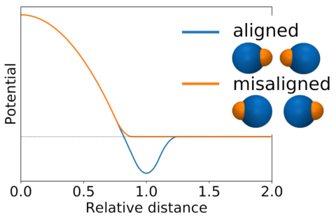 b.
b.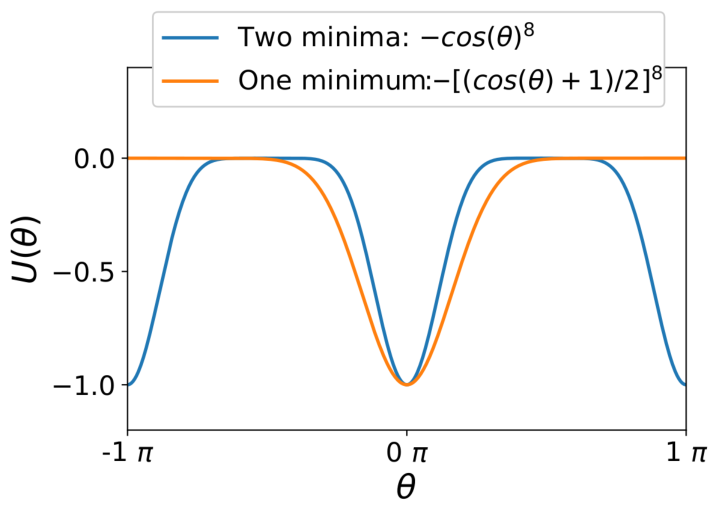 c.
c.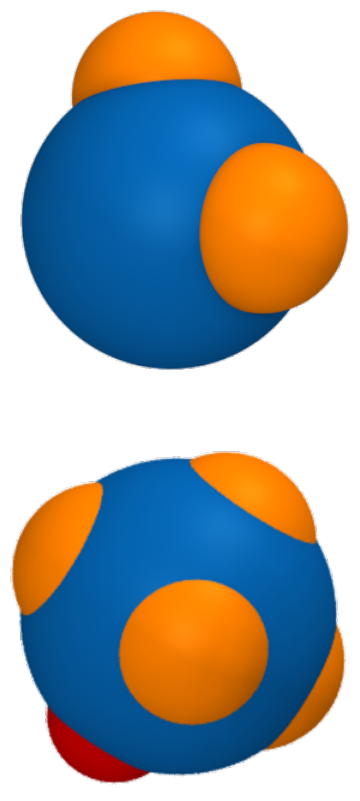
To validate MSM/RD schemes, we require an inexpensive model of molecules capable of representing complex behavior observed in realistic MD systems such as: translational and rotational diffusion, position and orientation dependent pair interactions, orientation dependent binding, multiple binding sites and conformation switching. We can construct such a model based on patchy particles (klein2014studying; newton2015rotational; schluttig2008dynamics). We model molecules as diffusive spherical particles with an isotropic repulsive potential to avoid overlapping; an attractive isotropic part can also be incorporated. Patches are then placed on the surface of the particles, and each patch produces a short-range attractive potential with patches from other particles, generating translational and rotational motion (vijaykumar2017multiscale). The potential energy between patch of particle and patch of particle can be decomposed into two parts. The first part depends only on the relative distance between the patches, , and the types of the patches. It corresponds to an attractive force that pulls patches together . The second part depends on the relative orientation, , of the particles, and it is activated if two patches are close enough to each other. This will favor specific relative orientations for the different bindings between patches. In all the models used for this work, the overall interaction potential between two particles, and , can be written in the following form:
where runs over the patches of particle and runs over the patches of particle . and are the total number of patches of and respectively. In general, particle and can both have conformational changes; each combination of conformations is allowed to have a completely different potential energy. In this work, conformation changes will correspond to turning on and off specific patches. Figure 2 shows the potential between a pair of patchy particles with one patch, as well as examples of orientation dependent potentials.
The position of the particles is simply given by the coordinates of the center of the sphere , and their orientation is given in terms of quaternions. In order to model the translational and orientational diffusion of one particle, we use overdamped Langevin dynamics. We assume the translational and rotational diffusion are independent and both isotropic, so we obtain
| (10) |
where is the orientation in the axis-angle representation, and are the translational and rotational damping coefficients; and the force and torque due to pair-interactions and external fields; is the conformation of the particle; and and each correspond to three-dimensional Gaussian white noise. The force can be rewritten in terms of the potential as ; the torque is convenient to leave explicitly since it is not trivial to write a potential in terms of axis-angle variables or quaternions. These two equations can be discretized using the Euler-Maruyama scheme (higham2001algorithmic) using a time-step .
| (11) |
The rotation represented by the change in axis-angle can be rewritten as a quaternion using Eq. 6. The new orientation is simply given by the quaternion product In each case, represents an independent three-dimensional vector with each entry a normal random variable with mean zero and variance . As the diffusion coefficients depend on the conformation, it is convenient to assume the switching of conformation is modeled with an MSM using a fixed lag-time that is a multiple of , a positive integer. This is not strictly required, but it simplifies the implementation since the conformation change occurs always at the end of a time step. The forces and torques are calculated directly from potential energies like the ones shown in Fig. 2.
This model satisfies all the requirements we established at the beginning of this section. It can be generalized to non-isotropic and coupled rotational and translational dynamics (delong2015brownian; schluttig2008dynamics), and molecules can even be modeled by multiple overlapping beads with reaction patches (schluttig2008dynamics).
IV. Results
a.![[Uncaptioned image]](2103.06889v4/patchyProtein_diagramV5.png) b.
b.![[Uncaptioned image]](2103.06889v4/patchyProtein_twoHist.png)
c.![[Uncaptioned image]](2103.06889v4/bound2bound__patchyProtein_FPTs_v3.png)
Illustrations and results of the MSM/RD scheme for the protein-protein system. a. MSM/RD sample trajectory. Particle diffuses with coefficient , and particle with coefficient or depending on its conformation. If the relative distance satisfies , we switch from the non-interacting to the transition regime. Here, the particles can transition to one of the six bound states with rate that depends on their relative configuration and the final bound state . From a bound state , the compound can transition to another bound state with rate or it can unbind to another relative configuration with rate . MSM/RD provides a piecewise constant approximation of all the configuration-dependent rates. b. Comparisons of first passage time (FPT) distributions between the benchmark and MSM/RD from an unbound state to any bound state and vice versa. Each distribution was calculated with simulations. c. Comparison of FPT distributions for all transitions between the six possible bound states, each calculated over simulations. The blue grid shows the relative error of the corresponding rates, , calculated as the inverse MFPT. The average percentage error is of while the maximum is of .
a.
 b.
b. c.
c.


![[Uncaptioned image]](2103.06889v4/ring_molecules_formation_v3.png)
Illustrations and multiparticle MSM/RD results for the formation of ring molecules. a. Diagram showing the formation of the trimeric, tetrameric and pentameric ring molecules. b. Comparisons of the FPT distributions obtained with multiparticle MSM/RD and the benchmark for the formation of the trimeric, tetrameric and pentemric ring molecules. The results were obtained from simulations for each case. c. Comparison of the rate at which a pentameric ring is generated for different molar concentrations. Each point was calculated as the inverse of the MFPT obtained from simulations; the error bars represent the standard deviation over bootstrapped samples.
To test and verify MSM/RD, we construct an MD benchmark model of molecules that is simple enough such that we can produce a large amount of data, but complex enough so it models complex behavior observed in realistic MD systems. This model is based on patchy particles (klein2014studying; newton2015rotational; schluttig2008dynamics); we model molecules as spherical particles with isotropic diffusion and an isotropic repulsive potential to avoid overlapping. Patches are then placed on the surface of the particles, and each patch produces a short-range configuration-dependent attractive potential with patches from other particles, generating translational and rotational motion, see the methods section for details. This model is the basis for all the benchmark models in this section.
In the following examples, it is not necessary to parametrize the diffusion operator since it is the same for both the benchmark and the MSM/RD simulation. This serves to isolate the dynamics of and validate the coupling mechanism. For general protein-protein systems, one needs to extract the diffusion coefficients/matrices from the MD data using well documented methods (bullerjahn2020optimal; linke2018fully) (SI Appendix D).
A. MSM/RD for protein-protein systems
The benchmark model consists of two molecules, and (Fig. IV. Resultsa), represented by different patchy particles. Particle has only one conformation and six binding patches: five of them have the same attraction potential (yellow), and the other one has a stronger attraction potential (red). Particle has two conformations. In one conformation (), it has one binding patch (red), and in the other one (, the patch is turned off, and it cannot bind. Each binding allows only one meta-stable relative orientation, yielding a total of six possible bound states. The diffusion of depends on its conformation, and it is visualized as a three-dimensional asterisk to distinguish its orientation. We illustrate an MSM/RD trajectory of the system on Fig. IV. Resultsa.
To parametrize the MSM/RD scheme, we simulate the benchmark MD model with specific settings to mimic a common MD simulation. We assume both molecules have a diameter of , which is a typical size for a real protein. We simulate using periodic boundary conditions and a cube with edge-length of as unit cell. Each simulation runs for time steps of each, yielding a total simulation time of . We run of these simulations independently, and we use them to parametrize the MSM/RD scheme following the steps illustrated in SI Appendix B.
In Fig. IV. Results, we compare the MSM/RD results against the MD benchmark. We calculate the first passage times (FPTs) of a given transition by running the benchmark and the MSM/RD simulations in equal conditions, and we run the same number of FPT samples for each model. Figure IV. Resultsb compares the FPTs distribution from the unbound state to any bound states and vice versa. The left panel of Fig. IV. Resultsc compares the FPT distributions for all the possible transitions between bound states. Note these transitions include pathways that start at a bound state, unbind completely and end in another bound state, so it is ideal to evaluate if the MSM/RD produces an accurate coupling. The right panel of Fig. IV. Resultsc shows the MSM/RD scheme percent error for the transition rates between bound states. Overall, MSM/RD can reproduce the dynamics of the MD benchmark with good accuracy.
B. MSM/RD for dimer of two-patch particle
The benchmark model consists of two identical molecules, each with two equally strong binding patches. The molecules can bind together through any of their two binding sites. Unlike the previous example, we allow for two meta-stable relative orientations per patch binding, allowing for a conformation change in the bound configuration.
As the molecules have two patches each, they can bind in four different ways; each of these has two stable relative orientations, so this system has a total of eight meta-stable bound states. However, as they are all identical, many of these eight states are indistinguishable from each other and can all be collapsed into two functional states, and . This is depicted graphically in Fig. 3a. Nonetheless, note each of these meta-stable states corresponds to a different relative position and orientation between the molecules. We parametrize the MSM/RD scheme with the same setup as in the protein-protein system example, see SI Appendix B.
In Fig. 3, we compare MSM/RD results against the MD benchmark. We calculate FPTs for both the MD benchmark and the MSM/RD simulations in equal conditions. In Fig. 3b, we show the binding rates as a function of concentration, where each binding rate is calculated as the inverse of the mean first passage time (MFPT). The concentration is adjusted by changing the edge-length of the simulation box, starting at and increasing for each point. In Fig. 3c, we compare the FPTs distributions for several relevant transitions. Even when the original simulations to parametrize the scheme ran for only the MSM/RD scheme produces excellent results for transitions with higher MFPTs.
C. Multiparticle MSM/RD: formation of pentameric ring
| Rate | Concentration | MD Benchmark | MSM/RD | % Error |
|---|---|---|---|---|
| 5.4% | ||||
| 4.5% | ||||
| 3.4% | ||||
| () | 6.3% | |||
| 5.7% | ||||
| 3.6% |
We develop and implement the first multiparticle MSM/RD scheme to study the formation of pentameric ring molecules (inspired by (klein2014studying)). The benchmark MD model is a modified version of the two-patch dimer model. It consists again of two identical molecules, each with two equally strong binding sites. Unlike the previous example, we only allow one meta-stable relative orientation per patch binding. We further increase the binding strength such that unbinding events are very rare and not observed in the timescales of interest. The particles can bind with each other forming chains, which eventually can close forming either trimeric, tetrameric or pentameric ring structures (Fig. IV. Resultsa).
We parametrize the MSM/RD scheme with the same setup as in the protein-protein system example, see SI Appendix B. The multiparticle MSM/RD scheme requires modifications to the two-particle MSM/RD algorithm. These modifications are shown in SI Appendix C. We further need to estimate the diffusion coefficients of the multiparticle chains. We employ standard methods to estimate them (SI Appendix D).
In Fig. IV. Resultsb, we compare MSM/RD results against the MD benchmark. We calculate FPTs for the formation of all the three ring molecules, using both the MD benchmark and the MSM/RD simulations in equal conditions: five particles with random positions and orientations placed in a simulation box of edge-length of nm with periodic boundaries. In Fig. 3c, we show the rate of formation of pentameric rings for different concentrations by changing the simulation box size. In Table 1, we show the exact values and relative errors of the rates plotted in Fig. IV. Resultsc.
Note MSM/RD is not as good at approximating the formation of trimeric and tetrameric rings (Fig. IV. Resultsb). This is due to MSM/RD modeling the particle-chains in steps 3 and 4 of Fig IV. Resultsa as a fixed structure, while in the MD benchmark the chain is flexible, allowing for patches to get closer together, which increases the rate at which the ring is closed. This could be fixed by using a new MSM to describe the dynamics between the three or four particle chains and an additional particle. Nonetheless, note the rates of formation of pentameric rings are not affected by these problem since they are conditioned on not having trimeric or tetrameric rings forming beforehand. In its current formulation, MSM/RD multiparticle implementations are limited to non-crowded environments since only pair interactions are parametrized. It is important to take these issues into account when implementing MSM/RD applications.
V. Discussion
We presented a coarse-grained model of molecular kinetics based on hybrid switching diffusions. With this model, we developed a robust framework for coupling Markov models of molecular kinetics with particle-based reaction diffusion (MSM/RD). Based on this framework, we derived one possible MSM/RD scheme by discretizing the underlying equation (Eq. 5), generalizing previous approaches (dibak2018msm). We implemented and verified it for three benchmark systems: the first two involve two protein-protein systems, while the third one is a multiparticle system to model the formation of pentameric molecules. We obtained an excellent agreement between the FPT distributions and reaction rates of relevant transitions.
The framework is well-suited to model protein-ligand binding in large domains and time-scales as in the previous work (dibak2018msm). Given enough data for the parametrization, it is also suited to model protein-protein dynamics since it incorporates arbitrary orientations, conformation switching and multiple binding sites. To parametrize the MSM/RD scheme for protein-protein systems, we would need the MD data of the two proteins interacting and individually, both in small simulation boxes. The interacting proteins data would serve to parametrize the scheme in the bound and transition regime, similarly to the works (BuchFabritiis_PNAS11_Binding; SilvaHuang_PlosCB_LaoBinding; PlattnerNoe_NatComm15_TrypsinPlasticity; PlattnerEtAl_NatChem17_BarBar) with the addition of the transition states, which might require a slightly larger box. The individual molecules data would serve to parametrize the scheme in the non-interacting regime. The resulting MSM/RD scheme could run simulations at much larger time- and length-scales than those allowed by MD.
The multiparticle implementation of MSM/RD has promising applications to the study of self-assembly of structures composed of several copies of the same molecule (or a small set of molecules), such as virus capsids (arkhipov2006stability) or soft matter self-assembly. This setting is ideal since we only need MD data of one pair (or a few pairs) of molecules in a small simulation box to parametrize an MSM/RD multiparticle simulation, which could potentially model the formation of the full capsid.
The main caveat of MSM/RD is that the parametrization requires a large amount of MD data, which is not yet possible to obtain for most systems of interest. However, given the increasing computational power, more and more systems will soon be within reach of MSM/RD. The scheme might also become less effective in the presence of long-ranged interactions, though it might be possible to incorporate them into the dynamics of the non-interacting-regime using coarse-grained potentials (davtyan2012awsem; wang2021multi). Finally, in its current form, the MSM/RD multiparticle implementation only takes into account pair interactions, and thus the scheme is not yet adequate for crowded multi-molecular environments.
Although application-dependent, one can expect MSM/RD to reduce computational cost by several orders of magnitude in comparison to MD. MD simulations propagate the position and velocity of every atom, which corresponds to several thousands of degrees of freedom in an average protein-protein simulation. MSM/RD only propagates two independent Brownian bodies together with an MSM. This corresponds to at most 14 degrees of freedom, 6 for the position/orientation and one for the MSM (per molecule). Finally, considering that MSM/RD can operate in larger domains with larger time steps, equivalent MD simulations would need to increase dramatically the number of solvent molecules yielding an exploding number of degrees of freedom, while still limited to small time steps.
Software
To enable reproducibility and implementation of this work, we developed the MSM/RD software package, a C++/python package. All the code and software developed for this work are open source and available under an MIT license in github.com/markovmodel/msmrd2 and Zenodo (delRazoMSMRD). The data used in this work was produced using the MSM/RD software.
We acknowledge support by the European Commission (ERC CoG 772230), German Ministry for Education and Research (Berlin Institute for the Foundations of Learning and Data BIFOLD), Deutsche Forschungsgemeinschaft (SFB1114/C03, SFB1114/A04 and TRR186/A12), the Berlin Mathematics research center Math+ (project AA1-6), and the Dutch Institute for Emergent Phenomena at the University of Amsterdam. M.J.R. thanks Hong Qian for helpful discussions over the course of this work. We also thank two anonymous reviewers that greatly improved the presentation of this work.
Data Availability
The data and scripts to produce the plots in this work are available in Zenodo (delRazoMSMRDdata). The complete dataset that support the findings of this study are available from the corresponding author upon reasonable request.
References
References
- (1) XS Xie, J Trautman, Single-molecule optical studies at room temperature. \JournalTitleAnnu. Rev. Phys. Chem 49, 441–480 (1998).
- (2) P Ao, C Kwon, H Qian, On the existence of potential landscape in the evolution of complex systems. \JournalTitleComplexity 12, 19–27 (2007).
- (3) JM Schurr, The role of diffusion in bimolecular solution kinetics. \JournalTitleBiophys. J. 10, 700 (1970).
- (4) K Burdzy, ZQ Chen, , et al., Discrete approximations to reflected Brownian motion. \JournalTitleAnn. Probab. 36, 698–727 (2008).
- (5) JA Schellman, Solvent denaturation. \JournalTitleBiopolymers 17, 1305–1322 (1978).
- (6) A Batakis, VH Nguyen, On the exit distribution of partially reflected Brownian motion in planar domains. \JournalTitlePotential Anal. 38, 537–548 (2013).
- (7) DS Grebenkov, Partially reflected brownian motion: a stochastic approach to transport phenomena. \JournalTitleFocus on Probab. Th., 135–169 (2006).
- (8) C Bustamante, In singulo biochemistry: When less is more. \JournalTitleAnnu. Rev. Biochem. 77, 45–50 (2008).
- (9) A Gräslund, R Rigler, J Widengren, Single Molecule Spectroscopy in Chemistry, Physics and Biology. (Springer), (2010).
- (10) H Qian, S Kou, Statistics and related topics in single-molecule biophysics. \JournalTitleAnnu. Rev. Statstics 1, 465–492 (2014).
- (11) EL Elson, WW Webb, Concentration correlation spectroscopy: a new biophysical probe based on occupation number fluctuations. \JournalTitleAnnu. Rev. Biophys. 4, 311–334 (1975).
- (12) MB Weissman, Fluctuation spectroscopy. \JournalTitleAnnu. Rev. Phys. Chem. 32, 205–232 (1981).
- (13) TL Hill, IW Plesner, Studies in irreversible thermodynamics. ii. a simple class of lattice models for open systems. \JournalTitleJ. Chem. Phys. 43, 267–285 (1965).
- (14) TL Hill, Approach of certain systems, including membranes, to steady state. \JournalTitleJ. Chem. Phys 54, 34–35 (1971).
- (15) P Hänggi, P Talkner, M Borkovec, Reaction-rate theory: Fifty years after kramers. \JournalTitleRev. Mod. Phys. 62, 251 (1990).
- (16) HA Kramers, Brownian motion in a field of force and the diffusion model of chemical reactions. \JournalTitlePhysica 7, 284–304 (1940).
- (17) M Delbrück, Statistical fluctuations in autocatalytic reactions. \JournalTitleJ. Chem. Phys 8, 120–124 (1940).
- (18) DT Gillespie, Stochastic simulation of chemical kinetics. \JournalTitleAnnu. Rev. Phys. Chem. 58, 35–55 (2007).
- (19) H Qian, Cellular biology in terms of stochastic nonlinear biochemical dynamics: Emergent properties, isogenetic variations and chemical system inheritability. \JournalTitleJ. Stat. Phys. 141, 990–1013 (2010).
- (20) R Rigler, ELe Elson, Fluorescence Correlation Spectroscopy: Theory and Applications. (Springer Series in Chemical Physics, vol. 65, New York), (2001).
- (21) G Feher, M Weissman, Fluctuation spectroscopy: Determination of chemical reaction kinetics from the frequency spectrum of fluctuations. \JournalTitleProc. Natl. Acad. Sci. U.S.A. 70, 870–875 (1973).
- (22) EL Elson, D Magde, Fluorescence correlation spectroscopy. i. conceptual basis and theory. \JournalTitleBiopolymers 13, 1–27 (1974).
- (23) L Onsager, S Machlup, Fluctuations and irreversible processes. \JournalTitlePhys. Rev. 91, 1505–1512 (1953).
- (24) M Lax, Fluctuations from the nonequilibrium steady state. \JournalTitleRev. Mod. Phys. 32, 25 (1960).
- (25) J Keizer, Statistical Thermodynamics of Nonequilibrium Processes. (Springer), (1987).
- (26) S Friess, Technique of organic chemistry, vol. viii, part ii: Investigation of rates and mechanisms of reactions. interscience, new york, 1963; m. eigen, l. de mayer, relax. \JournalTitleMethods, 895–1054 (year?).
- (27) L Onsager, Reciprocal relations in irreversible processes. ii. \JournalTitlePhys. Rev. 38, 2265 (1931).
- (28) D Magde, EL Elson, WW Webb, Thermodynamic fluctuations in a reacting system—measurement by fluorescence correlation spectroscopy. \JournalTitlePhys. Rev. Lett. 29, 705–708 (1972).
- (29) M Ehrenberg, R Rigler, Rotational brownian motion and fluorescence intensify fluctuations. \JournalTitleChem. Phys. 4, 390–401 (1974).
- (30) XS Xie, PJ Choi, GW Li, NK Lee, G Lia, Single-molecule approach to molecular biology in living bacterial cells. \JournalTitleAnnu. Rev. Biophys. 37, 417–444 (2008).
- (31) J Keizer, On the macroscopic equivalence of descriptions of fluctuations for chemical reactions. \JournalTitleJ. Math. Phys. 18, 1316–1321 (1977).
- (32) WK Ridgeway, DP Millar, JR Williamson, The spectroscopic basis of fluorescence triple correlation spectroscopy. \JournalTitleJ. Phys. Chem. B 116, 1908–1919 (2012).
- (33) H Mino, JT Rubinstein, JA White, Comparison of algorithms for the simulation of action potentials with stochastic sodium channels. \JournalTitleAnn. Biomed. Eng. 30, 578–587 (2002).
- (34) D Shoup, A Szabo, Role of diffusion in ligand binding to macromolecules and cell-bound receptors. \JournalTitleBiophys. J. 40, 33–39 (1982).
- (35) FC Collins, GE Kimball, Diffusion-controlled reaction rates. \JournalTitleJ. Colloid Sci. 4, 425–437 (1949).
- (36) SS Andrews, D Bray, Stochastic simulation of chemical reactions with spatial resolution and single molecule detail. \JournalTitlePhys. Biol. 1, 137 (2004).
- (37) SS Khokhlova, N Agmon, Comparison of alternate approaches for reversible geminate recombination. \JournalTitleBull. Korean Chem. Soc 33, 1021 (2012).
- (38) N Agmon, A Szabo, Theory of reversible diffusion-influenced reactions. \JournalTitleJ. Chem. Phys. 92, 5270–5284 (1990).
- (39) A Szabo, K Schulten, Z Schulten, First passage time approach to diffusion controlled reactions. \JournalTitleJ. Chem. Phys. 72, 4350–4357 (1980).
- (40) AV Popov, N Agmon, Three-dimensional simulations of reversible bimolecular reactions: The simple target problem. \JournalTitleJ. Chem. Phys. 115, 8921–8932 (2001).
- (41) AV Popov, N Agmon, Three-dimensional simulation verifies theoretical asymptotics for reversible binding. \JournalTitleChem. Phys. Lett. 340, 151–156 (2001).
- (42) H Kim, KJ Shin, Exact solution of the reversible diffusion-influenced reaction for an isolated pair in three dimensions. \JournalTitlePhys. Rev. Lett. 82, 1578–1581 (1999).
- (43) N Agmon, Diffusion with back reaction. \JournalTitleJ. Chem. Phys. 81, 2811–2817 (1984).
- (44) H Kim, KJ Shin, N Agmon, Excited-state reversible geminate recombination with quenching in one dimension. \JournalTitleJ. Chem. Phys 111, 3791–3799 (1999).
- (45) IV Gopich, KM Solntsev, N Agmon, Excited-state reversible geminate reaction. i. two different lifetimes. \JournalTitleJ. Chem. Phys 110, 2164–2174 (1999).
- (46) IV Gopich, A Szabo, Kinetics of reversible diffusion influenced reactions: the self-consistent relaxation time approximation. \JournalTitleJ. Chem. Phys. 117, 507–517 (2002).
- (47) J Hattne, D Fange, J Elf, Stochastic reaction-diffusion simulation with mesord. \JournalTitleBioinformatics 21, 2923–2924 (2005).
- (48) OG Berg, On diffusion-controlled dissociation. \JournalTitleChem. Phys. 31, 47–57 (1978).
- (49) A Einstein, Investigations on the Theory of the Brownian Movement. (Courier Dover Publications), (1956).
- (50) GE Uhlenbeck, LS Ornstein, On the theory of the brownian motion. \JournalTitlePhys. Rev. 36, 823 (1930).
- (51) Mv Smoluchowski, Versuch einer mathematischen theorie der koagulationskinetik kolloider lösungen. \JournalTitleZ. Phys. Chem 92, 9 (1917).
- (52) GN Lewis, A new principle of equilibrium. \JournalTitleProc. Natl. Acad. Sci. U.S.A. 11, 179 (1925).
- (53) JS van Zon, PR Ten Wolde, Simulating biochemical networks at the particle level and in time and space: Green’s function reaction dynamics. \JournalTitlePhys. Rev. Lett. 94, 128103 (2005).
- (54) H Qian, Nonlinear stochastic dynamics of mesoscopic homogeneous biochemical reaction systems — An analytical theory. \JournalTitleNonlinearity 24, R19–R49 (2011).
- (55) H Qian, LM Bishop, The chemical master equation approach to nonequilibrium steady-state of open biochemical systems: linear single-molecule enzyme kinetics and nonlinear biochemical reaction networks. \JournalTitleInt. J. Mol. Sci. 11, 3472–3500 (2010).
- (56) M Vellela, H Qian, Stochastic dynamics and non-equilibrium thermodynamics of a bistable chemical system: the schlögl model revisited. \JournalTitleJ. R. Soc. Interface 6, 925–940 (2009).
- (57) P Langevin, Sur la théorie du mouvement brownien. \JournalTitleCR Acad. Sci. Paris 146 (1908).
- (58) DC Torney, HM McConnell, Diffusion-limited reactions in one dimension. \JournalTitleJ. Phys. Chem. 87, 1941–1951 (1983).
- (59) DC Torney, HM McConnell, Diffusion-limited reaction rate theory for two-dimensional systems. \JournalTitleProc. R. Soc. London, Ser. A 387, 147–170 (1983).
- (60) GH Weiss, Overview of theoretical models for reaction rates. \JournalTitleJ. Stat. Phys. 42, 3–36 (1986).
- (61) T Sokolowski, L Bossen, T Miedema, N Becker, Green’s function reaction dynamics—an exact and efficient way to simulate intracellular pattern formation in ICNAAM 2010: International Conference of Numerical Analysis and Applied Mathematics 2010. (AIP Publishing), Vol. 1281, pp. 1342–1345 (2010).
- (62) PG Saffman, M Delbrück, Brownian motion in biological membranes. \JournalTitleProc. Natl. Acad. Sci. U.S.A. 72, 3111–3113 (1975).
- (63) T Prüstel, M Meier-Schellersheim, Exact green’s function of the reversible diffusion-influenced reaction for an isolated pair in two dimensions. \JournalTitleJ. Chem. Phys. 137, 054104 (2012).
- (64) T Prüstel, M Meier-Schellersheim, Theory of reversible diffusion-influenced reactions with non-markovian dissociation in two space dimensions. \JournalTitleJ. Chem. Phys. 138, 104112 (2013).
- (65) T Prüstel, M Meier-Schellersheim, Rate coefficients, binding probabilities, and related quantities for area reactivity models. \JournalTitleJ. Chem. Phys. 141, 194115 (2014).
- (66) J Feng, The hydrodynamic limit for the reaction diffusion equation- an approach in terms of the GPV method. \JournalTitleJ. of Theor. Probab. 9, 285–299 (1996).
- (67) L Arnold, On the consistency of the mathematical models of chemical reactions in Dynamics of synergetic systems. (Springer), pp. 107–118 (1980).
- (68) H Qian, An asymptotic comparative analysis of the thermodynamics of non-covalent association. \JournalTitleJ. Math. Biol. 41, 331–340 (2000).
- (69) B Drawert, S Engblom, A Hellander, URDME: a modular framework for stochastic simulation of reaction-transport processes in complex geometries. \JournalTitleBMC Syst. Biol. 6, 76 (2012).
- (70) J Schöneberg, F Noé, Readdy-a software for particle-based reaction-diffusion dynamics in crowded cellular environments. \JournalTitlePloS one 8, e74261 (2013).
- (71) M Tomita, et al., E-cell: software environment for whole-cell simulation. \JournalTitleBioinformatics 15, 72–84 (1999).
- (72) S Wils, E De Schutter, STEPS: Modeling and simulating complex reaction-diffusion systems with Python. \JournalTitleFront. Neuroinf. 3, art. no. 15 (2009).
- (73) SK Godunov, A difference method for numerical calculation of discontinuous solutions of the equations of hydrodynamics. \JournalTitleMatematicheskii Sbornik 89, 271–306 (1959).
- (74) J Raynal, Computing as a language of physics. \JournalTitleIAEA, Vienna 281 (1972).
- (75) JD Murray, Mathematical Biology I: An Introduction, vol. 17 of Interdisciplinary Applied Mathematics. (Springer, New York, NY, USA,), (2002).
- (76) RJ LeVeque, Finite volume methods for hyperbolic problems. (Cambridge university press) Vol. 31, (2002).
- (77) Clawpack Development Team, Clawpack software (2014) Version 5.0.
- (78) EF Toro, Riemann Solvers and Numerical Methods for Fluid Dynamics. (Springer), (2008).
- (79) SA Isaacson, Relationship between the reaction–diffusion master equation and particle tracking models. \JournalTitleJ. Phys. A: Math. Theor. 41, 065003 (2008).
- (80) SA Isaacson, A convergent reaction-diffusion master equation. \JournalTitleJ. Chem. Phys. 139, 054101 (2013).
- (81) S Hellander, A Hellander, L Petzold, Reaction rates for mesoscopic reaction-diffusion kinetics. \JournalTitlePhys. Rev. E 91, 023312 (2015).
- (82) M Doi, Stochastic theory of diffusion-controlled reaction. \JournalTitleJ. Phys. A: Math. Gen. 9, 1479 (1976).
- (83) H Wang, CS Peskin, TC Elston, A robust numerical algorithm for studying biomolecular transport processes. \JournalTitleJ. Theor. Biol. 221, 491–511 (2003).
- (84) K Takahashi, S Tănase-Nicola, PR Ten Wolde, Spatio-temporal correlations can drastically change the response of a mapk pathway. \JournalTitleProc. Natl. Acad. Sci. U.S.A. 107, 2473–2478 (2010).
- (85) A Donev, et al., A first-passage kinetic monte carlo algorithm for complex diffusion–reaction systems. \JournalTitleJ. Comput. Phys. 229, 3214–3236 (2010).
- (86) RJ LeVeque, Finite Difference Methods for Ordinary and Partial Differential Equations: Steady State and Time Dependent Problems. (Cambridge University Press), (2007).
- (87) H Qian, Phosphorylation energy hypothesis: open chemical systems and their biological functions. \JournalTitleAnnu. Rev. Phys. Chem. 58, 113–142 (2007).
- (88) A Szabo, Theory of diffusion-influenced fluorescence quenching. \JournalTitleJ. Phys. Chem. 93, 6929–6939 (1989).
- (89) D Fange, OG Berg, P Sjöberg, J Elf, Stochastic reaction-diffusion kinetics in the microscopic limit. \JournalTitleProc. Natl. Acad. Sci. U.S.A. 107, 19820–19825 (2010).
- (90) MJ del Razo, W Pan, H Qian, G Lin, Fluorescence correlation spectroscopy and nonlinear stochastic reaction–diffusion. \JournalTitleThe Journal of Physical Chemistry B 118, 7037–7046 (2014).
- (91) RA Marcus, N Sutin, Electron transfers in chemistry and biology. \JournalTitleBiochim. Biophys. Acta, Rev. Bioenerg. 811, 265–322 (1985).
- (92) TM Bartol Jr, B Land, EE Salpeter, MM Salpeter, Monte carlo simulation of miniature endplate current generation in the vertebrate neuromuscular junction. \JournalTitleBiophys. J. 59, 1290 (1991).
- (93) E Pines, D Huppert, N Agmon, Geminate recombination in excited-state proton-transfer reactions: Numerical solution of the debye–smoluchowski equation with backreaction and comparison with experimental results. \JournalTitleJ. Chem. Phys. 88, 5620–5630 (1988).
- (94) EB Krissinel’, N Agmon, Spherical symmetric diffusion problem. \JournalTitleJ. Comput. Chem. 17, 1085–1098 (1996).
- (95) B Oksendal, Stochastic differential equations: an introduction with applications. (Springer Science & Business Media), (2013).
- (96) JS van Zon, PR ten Wolde, Green’s-function reaction dynamics: a particle-based approach for simulating biochemical networks in time and space. \JournalTitleJ. Chem. Phys. 123, 234910 (2005).
- (97) MJ del Razo, H Qian, A discrete stochastic formulation for reversible bimolecular reactions via diffusion encounter. \JournalTitleCommunications in Mathematical Sciences 14, 1741–1772 (2016).
- (98) WJ Heuett, H Qian, Grand canonical markov model: a stochastic theory for open nonequilibrium biochemical networks. \JournalTitleThe Journal of chemical physics 124, 044110 (2006).
- (99) J Keizer, Nonequilibrium statistical thermodynamics and the effect of diffusion on chemical reaction rates. \JournalTitleThe Journal of Physical Chemistry 86, 5052–5067 (1982).
- (100) J Keizer, Theory of rapid bimolecular reactions in solution and membranes. \JournalTitleAccounts of Chemical Research 18, 235–241 (1985).
- (101) J Keizer, Diffusion effects on rapid bimolecular chemical reactions. \JournalTitleChemical Reviews 87, 167–180 (1987).
- (102) J Keizer, Statistical thermodynamics of nonequilibrium processes. (Springer Science & Business Media), (1987).
- (103) A Szabo, NS Ostlund, Modern quantum chemistry: introduction to advanced electronic structure theory. (Courier Corporation), (1989).
- (104) TG Kurtz, The relationship between stochastic and deterministic models for chemical reactions. \JournalTitleThe Journal of Chemical Physics 57, 2976–2978 (1972).
- (105) TG Kurtz, Limit theorems for sequences of jump markov processes approximating ordinary differential processes. \JournalTitleJournal of Applied Probability 8, 344–356 (1971).
- (106) D Reguera, J Rubi, J Vilar, The mesoscopic dynamics of thermodynamic systems. \JournalTitleThe Journal of Physical Chemistry B 109, 21502–21515 (2005).
- (107) D Bedeaux, I Pagonabarraga, JO De Zárate, J Sengers, S Kjelstrup, Mesoscopic non-equilibrium thermodynamics of non-isothermal reaction-diffusion. \JournalTitlePhysical Chemistry Chemical Physics 12, 12780–12793 (2010).
- (108) R Pathria, P Beale, Statistical Mechanics. (Elsevier Science), (1996).
- (109) C Kim, A Nonaka, JB Bell, AL Garcia, A Donev, Stochastic simulation of reaction-diffusion systems: A fluctuating-hydrodynamics approach. \JournalTitleThe Journal of Chemical Physics 146, 124110 (2017).
- (110) DF Anderson, TG Kurtz, Stochastic analysis of biochemical systems. (Springer) Vol. 1, (2015).
- (111) DJ Higham, An algorithmic introduction to numerical simulation of stochastic differential equations. \JournalTitleSIAM review 43, 525–546 (2001).
- (112) WA Catterall, Voltage-gated calcium channels. \JournalTitleCold Spring Harbor perspectives in biology 3, a003947 (2011).
- (113) S Barnes, ME Kelly, Calcium channels at the photoreceptor synapse in Photoreceptors and calcium. (Springer), pp. 465–476 (2002).
- (114) SM Bajjalieh, RH Scheller, The biochemistry of neurotransmitter secretion. \JournalTitleJournal of Biological Chemistry 270, 1971–1974 (1995).
- (115) X Mao, C Yuan, Stochastic differential equations with Markovian switching. (Imperial College Press), (2006).
- (116) G Yin, C Zhu, Hybrid switching diffusions: properties and applications. (Springer New York) Vol. 63, (2010).
- (117) NV Buchete, G Hummer, Coarse master equations for peptide folding dynamics. \JournalTitleJ. Phys. Chem. B 112, 6057–6069 (2008).
- (118) BE Husic, VS Pande, Markov state models: From an art to a science. \JournalTitleJ. Am. Chem. Soc. 140, 2386–2396 (2018).
- (119) HC Klein, US Schwarz, Studying protein assembly with reversible brownian dynamics of patchy particles. \JournalTitleJ. Chem. Phys. 140, 05B612_1 (2014).
- (120) S Delong, F Balboa Usabiaga, A Donev, Brownian dynamics of confined rigid bodies. \JournalTitleJ. Chem. Phys. 143, 144107 (2015).
- (121) A Vijaykumar, TE Ouldridge, PR ten Wolde, PG Bolhuis, Multiscale simulations of anisotropic particles combining molecular dynamics and green’s function reaction dynamics. \JournalTitleJ. Chem. Phys. 146, 114106 (2017).
- (122) DC Rapaport, Molecular dynamics simulation using quaternions. \JournalTitleJ. Comput. Phys. 60, 306–314 (1985).
- (123) M Dibak, MJ del Razo, D De Sancho, C Schütte, F Noé, MSM/RD: Coupling markov state models of molecular kinetics with reaction-diffusion simulations. \JournalTitleJ. Chem. Phys. 148, 214107 (2018).
- (124) R Zwanzig, Nonlinear generalized langevin equations. \JournalTitleJ. Stat. Phys. 9, 215–220 (1973).
- (125) G Ford, M Kac, P Mazur, Statistical mechanics of assemblies of coupled oscillators. \JournalTitleJ. Math. Phys. 6, 504–515 (1965).
- (126) P Leopardi, A partition of the unit sphere into regions of equal area and small diameter. \JournalTitleElectron. Trans. Numer. Anal. 25, 309–327 (2006).
- (127) RC Bernardi, MC Melo, K Schulten, Enhanced sampling techniques in molecular dynamics simulations of biological systems. \JournalTitleBiochim. Biophys. Acta, Gen. Subj. 1850, 872–877 (2015).
- (128) IV Gopich, A Szabo, Reversible stochastically gated diffusion-influenced reactions. \JournalTitleJ. Phys. Chem. B 120, 8080–8089 (2016).
- (129) AV Popov, N Agmon, IV Gopich, A Szabo, Influence of diffusion on the kinetics of excited-state association–dissociation reactions: Comparison of theory and simulation. \JournalTitleJ. Chem. Phys. 120, 6111–6116 (2004).
- (130) PC Bressloff, Stochastic switching in biology: from genotype to phenotype. \JournalTitleJ. Phys. A: Math. Theor. 50, 133001 (2017).
- (131) PC Bressloff, JN Maclaurin, Stochastic hybrid systems in cellular neuroscience. \JournalTitleJ. of Math. Neurosci. 8, 1–71 (2018).
- (132) PC Bressloff, SD Lawley, Hybrid colored noise process with space-dependent switching rates. \JournalTitlePhys. Rev. E 96, 012129 (2017).
- (133) PC Bressloff, SD Lawley, Stochastically gated diffusion-limited reactions for a small target in a bounded domain. \JournalTitlePhys. Rev. E 92, 062117 (2015).
- (134) PC Bressloff, SD Lawley, P Murphy, Protein concentration gradients and switching diffusions. \JournalTitlePhysical Review E 99, 032409 (2019).
- (135) M Hoffmann, C Fröhner, F Noé, Readdy 2: Fast and flexible software framework for interacting-particle reaction dynamics. \JournalTitlePLoS Comput. Biol. 15, e1006830 (2019).
- (136) MJ del Razo, H Qian, F Noé, Grand canonical diffusion-influenced reactions: A stochastic theory with applications to multiscale reaction-diffusion simulations. \JournalTitleThe Journal of Chemical Physics 149, 044102 (2018).
- (137) M Dibak, C Fröhner, F Noé, F Höfling, Diffusion-influenced reaction rates in the presence of pair interactions. \JournalTitleThe Journal of chemical physics 151, 164105 (2019).
- (138) C Fröhner, F Noé, Reversible interacting-particle reaction dynamics. \JournalTitleThe Journal of Physical Chemistry B 122, 11240–11250 (2018).
- (139) Z Schuss, A Singer, D Holcman, The narrow escape problem for diffusion in cellular microdomains. \JournalTitleProceedings of the National Academy of Sciences 104, 16098–16103 (2007).
- (140) A Szabo, D Shoup, SH Northrup, JA McCammon, Stochastically gated diffusion-influenced reactions. \JournalTitleJ. Chem. Phys. 77, 4484–4493 (1982).
- (141) H Wu, A Mardt, L Pasquali, F Noe, Deep generative markov state models in Adv. Neural Inf. Process. Syst. pp. 3975–3984 (2018).
- (142) D Kleinhans, R Friedrich, A Nawroth, J Peinke, An iterative procedure for the estimation of drift and diffusion coefficients of langevin processes. \JournalTitlePhys. Lett. A 346, 42–46 (2005).
- (143) BP Rao, Statistical inference for diffusion type processes. (Arnold London) Vol. 355, (1999).
- (144) YA Kutoyants, Statistical inference for ergodic diffusion processes. (Springer Science & Business Media), (2013).
- (145) H Sørensen, Parametric inference for diffusion processes observed at discrete points in time: a survey. \JournalTitleInt. Stat. Rev. 72, 337–354 (2004).
- (146) M Linke, J Köfinger, G Hummer, Fully anisotropic rotational diffusion tensor from molecular dynamics simulations. \JournalTitleJ. Phys. Chem. B 122, 5630–5639 (2018).
- (147) JT Bullerjahn, S von Bülow, G Hummer, Optimal estimates of self-diffusion coefficients from molecular dynamics simulations. \JournalTitleJ. Chem. Phys. 153, 024116 (2020).
- (148) H Qian, MP Sheetz, EL Elson, Single particle tracking. analysis of diffusion and flow in two-dimensional systems. \JournalTitleBiophys. J. 60, 910–921 (1991).
- (149) A Arkhipov, PL Freddolino, K Schulten, Stability and dynamics of virus capsids described by coarse-grained modeling. \JournalTitleStructure 14, 1767–1777 (2006).
- (150) M Kostré, C Schütte, F Noé, MJ del Razo, Coupling particle-based reaction-diffusion simulations with reservoirs mediated by reaction-diffusion pdes. \JournalTitlearXiv preprint arXiv:2006.00003 - (2020).
- (151) AC Newton, J Groenewold, WK Kegel, PG Bolhuis, Rotational diffusion affects the dynamical self-assembly pathways of patchy particles. \JournalTitleProc. Natl. Acad. Sci. U.S.A. 112, 15308–15313 (2015).
- (152) A Vijaykumar, PG Bolhuis, PR ten Wolde, Combining molecular dynamics with mesoscopic green’s function reaction dynamics simulations. \JournalTitleJ. Chem. Phys. 143, 214102 (2015).
- (153) L Delle Site, M Praprotnik, Molecular systems with open boundaries: Theory and simulation. \JournalTitlePhys. Rep. 693, 1–56 (2017).
- (154) A Agarwal, J Zhu, C Hartmann, H Wang, L Delle Site, Molecular dynamics in a grand ensemble: Bergmann–lebowitz model and adaptive resolution simulation. \JournalTitleNew Journal of Physics 17, 083042 (2015).
- (155) L Delle Site, et al., Molecular dynamics of open systems: Construction of a mean-field particle reservoir. \JournalTitleAdv. Theory Simul. 2, 1900014 (2019).
- (156) J Schluttig, D Alamanova, V Helms, US Schwarz, Dynamics of protein-protein encounter: A langevin equation approach with reaction patches. \JournalTitleJ. Chem. Phys. 129, 10B616 (2008).
- (157) MJ del Razo, M Dibak, C Schütte, F Noé, MSM/RD software (2021) http://dx.doi.org/10.5281/zenodo.4596416.
- (158) BR Jagger, SE Kochanek, S Haldar, RE Amaro, AJ Mulholland, Multiscale simulation approaches to modeling drug–protein binding. \JournalTitleCurr. Opin. Struct. Biol. 61, 213–221 (2020).
- (159) LW Votapka, BR Jagger, AL Heyneman, RE Amaro, SEEKR: simulation enabled estimation of kinetic rates, a computational tool to estimate molecular kinetics and its application to trypsin–benzamidine binding. \JournalTitleJ. Phys. Chem. B 121, 3597–3606 (2017).
- (160) BR Jagger, CT Lee, RE Amaro, Quantitative ranking of ligand binding kinetics with a multiscale milestoning simulation approach. \JournalTitleJ. Phys. Chem. Lett. 9, 4941–4948 (2018).
- (161) W Lim, B Mayer, T Pawson, Cell signaling. (Taylor & Francis), (2014).
- (162) RA Bradshaw, EA Dennis, Handbook of cell signaling. (Academic press), (2009).
- (163) JT Hancock, Cell signalling. (Oxford University Press), (2017).
- (164) T Hempel, et al., Independent markov decomposition: Towards modeling kinetics of biomolecular complexes. \JournalTitleProc. Natl. Acad. Sci. U.S.A. 118 (2021).
- (165) A Davtyan, et al., Awsem-md: protein structure prediction using coarse-grained physical potentials and bioinformatically based local structure biasing. \JournalTitleJ. Phys. Chem. B 116, 8494–8503 (2012).
- (166) J Wang, et al., Multi-body effects in a coarse-grained protein force field. \JournalTitleJ. Chem. Phys. 154, 164113 (2021).
- (167) MJ del Razo, M Dibak, C Schütte, F Noé, MSM/RD generated data/plots (2021) http://dx.doi.org/10.5281/zenodo.5236640.
- (168) G Froyland, K Padberg-Gehle, Ergodic Theory, Open Dynamics, and Coherent Structures, eds. W Bahsoun, C Bose, G Froyland. (Springer), pp. 171–216 (2014).
- (169) S Olsson, F Noé, Mechanistic models of chemical exchange induced relaxation in protein nmr. \JournalTitleJ. Am. Chem. Soc. 139, 200–210 (2017).
- (170) A Mardt, L Pasquali, H Wu, F Noé, VAMPnets for deep learning of molecular kinetics. \JournalTitleNat. Commun. 9, 5 (2018).
- (171) S Olsson, H Wu, F Paul, C Clementi, F Noé, Combining experimental and simulation data of molecular processes via augmented markov models. \JournalTitleProc. Natl. Acad. Sci. USA 114, 8265–8270 (2017).
- (172) JD Chodera, F Noé, Markov state models of biomolecular conformational dynamics. \JournalTitleCurr. Opin. Struc. Biol. 25, 135–144 (2014).
- (173) S Klus, et al., Data-driven model reduction and transfer operator approximation. \JournalTitleJ. Nonlinear Sci., 1–26 (2017).
- (174) H Wu, F Noé, Variational approach for learning markov processes from time series data. \JournalTitlearXiv:1707.04659 (2017).
- (175) M Gunkel, et al., Higher-order architecture of rhodopsin in intact photoreceptors and its implication for phototransduction kinetics. \JournalTitleStructure 23, 628–638 (2015).
- (176) J Biedermann, A Ullrich, J Schöneberg, F Noé, Readdymm: Fast interacting particle reaction-diffusion simulations using graphical processing units. \JournalTitleBiophys. J. 108, 457–461 (2015).
- (177) A Ullrich, et al., Dynamical organization of syntaxin-1a at the presynaptic active zone. \JournalTitlePLoS Comput. Biol. 11, e1004407 (2015).
- (178) F Noé, C Clementi, Collective variables for the study of long-time kinetics from molecular trajectories: theory and methods. \JournalTitleCurr. Opin. Struc. Biol. 43, 141–147 (2017).
- (179) GR Bowman, VS Pande, F Noé, eds., , Advances in Experimental Medicine and Biology. (Springer Heidelberg) Vol. 797, (2014).
- (180) F Nüske, H Wu, C Wehmeyer, C Clementi, F Noé, Markov state models from short non-equilibrium simulations - analysis and correction of estimation bias. \JournalTitlearXiv:1701.01665 (2017).
- (181) H Wu, F Noé, Spectral learning of dynamic systems from nonequilibrium data. \JournalTitleNIPS 29, 4179–4187 (2016).
- (182) F Paul, et al., Protein-ligand kinetics on the seconds timescale from atomistic simulations. \JournalTitleNat. Commun. 8, 1095 (2017).
- (183) N Plattner, S Doerr, GD Fabritiis, F Noé, Complete protein–protein association kinetics in atomic detail revealed by molecular dynamics simulations and markov modelling. \JournalTitleNat. Chem. 9, 1005–1011 (2017).
- (184) M Wieczorek, et al., Mhc class ii complexes sample intermediate states along the peptide exchange pathway. \JournalTitleNat. Commun. 7, 13224 (2016).
- (185) J Schöneberg, et al., Lipid-mediated px-bar domain recruitment couples local membrane constriction to endocytic vesicle fission. \JournalTitleNat. Commun. 8, 15873 (2017).
- (186) Y Posor, et al., Spatiotemporal control of endocytosis by phosphatidylinositol-3,4-bisphosphate. \JournalTitleNature 499, 233–237 (2013).
- (187) H Wu, et al., Variational koopman models: slow collective variables and molecular kinetics from short off-equilibrium simulations. \JournalTitleJ. Chem. Phys. 146, 154104 (2017).
- (188) G Perez-Hernandez, F Noé, Hierarchical time-lagged independent component analysis: computing slow modes and reaction coordinates for large molecular systems. \JournalTitleJ. Chem. Theory Comput. 12, 6118–6129 (2016).
- (189) F Noé, R Banisch, C Clementi, Commute maps: separating slowly-mixing molecular configurations for kinetic modeling. \JournalTitleJ. Chem. Theory Comput. 12, 5620–5630 (2016).
- (190) H Wu, F Paul, C Wehmeyer, F Noé, Multiensemble markov models of molecular thermodynamics and kinetics. \JournalTitleProc. Natl. Acad. Sci. USA 113, E3221–E3230 (2016).
- (191) S Doerr, MJ Harvey, F Noé, GD Fabritiis, HTMD: High-Throughput Molecular Dynamics for Molecular Discovery. \JournalTitleJ. Chem. Theory Comput. 12, 1845–1852 (2016).
- (192) W Wojtas-Niziurski, Y Meng, B Roux, S Bernèche, Self-learning adaptive umbrella sampling method for the determination of free energy landscapes in multiple dimensions. \JournalTitleJ. Chem. Theory Comput. 9, 1885–1895 (2013).
- (193) L Boninsegna, G Gobbo, F Noé, C Clementi, Investigating molecular kinetics by variationally optimized diffusion maps. \JournalTitleJ. Chem. Theory Comput. 11, 5947–5960 (2015).
- (194) MK Scherer, et al., PyEMMA 2: A software package for estimation, validation and analysis of Markov models. \JournalTitleJ. Chem. Theory Comput. 11, 5525–5542 (2015).
- (195) F Nüske, R Schneider, F Vitalini, F Noé, Variational tensor approach for approximating the rare-event kinetics of macromolecular systems. \JournalTitleJ. Chem. Phys. 144, 054105 (2016).
- (196) F Vitalini, F Noé, BG Keller, A basis set for peptides for the variational approach to conformational kinetics. \JournalTitleJ. Chem. Theory Comput. 11, 3992–4004 (2015).
- (197) B Trendelkamp-Schroer, F Noé, Efficient estimation of rare-event kinetics. \JournalTitlePhys. Rev. X (in press), preprint at arXiv:1409.6439 (2015).
- (198) F Noé, C Clementi, Kinetic distance and kinetic maps from molecular dynamics simulation. \JournalTitleJ. Chem. Theory Comput. 11, 5002–5011 (2015).
- (199) F Noé, Statistical inefficiency of markov model count matrices. \JournalTitlePreprint: http://publications.mi.fu-berlin.de/1699/ (2015).
- (200) TF Reubold, et al., Crystal structure of the dynamin tetramer. \JournalTitleNature 525, 404–408 (2015).
- (201) N Plattner, F Noé, Protein conformational plasticity and complex ligand binding kinetics explored by atomistic simulations and markov models. \JournalTitleNat. Commun. 6, 7653 (2015).
- (202) J Schöneberg, M Heck, KP Hofmann, F Noé, Explicit spatio-temporal simulation of receptor-g protein coupling in rod cell disk membranes. \JournalTitleBiophys. J. 107, 1042–1053 (2014).
- (203) H Wu, ASJS Mey, E Rosta, F Noé, Statistically optimal analysis of state-discretized trajectory data from multiple thermodynamic states. \JournalTitleJ. Chem. Phys. 141, 214106 (2014).
- (204) F Vitalini, ASJS Mey, F Noé, BG Keller, Dynamic properties of force fields. \JournalTitleJ. Chem. Phys. 142, 084101 (2015).
- (205) B Trendelkamp-Schroer, H Wu, F Paul, F Noé, Estimation and uncertainty of reversible markov models. \JournalTitleJ. Chem. Phys. 143, 174101 (2015).
- (206) J Schöneberg, F Noé, Readdy - a software for particle based reaction diffusion dynamics in crowded cellular environments. \JournalTitlePLoS ONE 8 (2013).
- (207) H Wu, F Noé, Gaussian markov transition models of molecular kinetics. \JournalTitleJ. Chem. Phys. 142, 084104 (2015).
- (208) GR Bowman, VS Pande, F Noé, eds., An Introduction to Markov State Models and Their Application to Long Timescale Molecular Simulation., Advances in Experimental Medicine and Biology. (Springer Heidelberg) Vol. 797, (2014).
- (209) F Nüske, BG Keller, G Pérez-Hernández, ASJS Mey, F Noé, Variational approach to molecular kinetics. \JournalTitleJ. Chem. Theory Comput. 10, 1739–1752 (2014).
- (210) H Wu, F Noé, Optimal estimation of free energies and stationary densities from multiple biased simulations. \JournalTitleMultiscale Model. Simul. 12, 25–54 (2014).
- (211) ASJS Mey, H Wu, F Noé, xTRAM: Estimating equilibrium expectations from time-correlated simulation data at multiple thermodynamic states. \JournalTitlePhys. Rev. X 4, 041018 (2014).
- (212) F Noé, H Wu, JH Prinz, N Plattner, Projected and hidden markov models for calculating kinetics and metastable states of complex molecules. \JournalTitleJ. Chem. Phys. 139, 184114 (2013).
- (213) B Trendelkamp-Schroer, F Noé, Efficient bayesian estimation of markov model transition matrices with given stationary distribution. \JournalTitleJ. Phys. Chem. 138, 164113. (2013).
- (214) F Noé, F Nüske, A variational approach to modeling slow processes in stochastic dynamical systems. \JournalTitleMultiscale Model. Simul. 11, 635–655 (2013).
- (215) SK Sadiq, F Noé, G De Fabritiis, Kinetic characterization of the critical step in HIV-1 protease maturation. \JournalTitleProc. Natl. Acad. Sci. USA 109, 20449–20454 (2012).
- (216) G Perez-Hernandez, F Paul, T Giorgino, G D Fabritiis, F Noé, Identification of slow molecular order parameters for markov model construction. \JournalTitleJ. Chem. Phys. 139, 015102 (2013).
- (217) B Lindner, Z Yi, JH Prinz, JC Smith, F Noé, Dynamic Neutron Scattering from Conformational Dynamics I: Theory and Markov models. \JournalTitleJ. Chem. Phys. 139, 175101 (2013).
- (218) Y Zheng, B Lindner, JH Prinz, F Noé, JC Smith, Dynamic Neutron Scattering from Conformational Dynamics II: Application using Molecular Dynamics Simulation and Markov modeling. \JournalTitleJ. Chem. Phys 139, 175102 (2013).
- (219) M Held, F Noé, Calculating kinetics and pathways of protein-ligand association. \JournalTitleEur. J. Cell Biol. (in press, doi:10.1016/j.ejcb.2011.08.004) (2011).
- (220) T Splettstößer, K Holmes, F Noé, JC Smith, Construction and simulation analysis of an improved structural model of the actin filament. \JournalTitleProteins 79, 2033– 2043 (2011).
- (221) H Wu, F Noé, A flat dirichlet process switching model for bayesian estimation of hybrid systems. \JournalTitleProc. Comput. Sci. 4, 1393–1402 (2011).
- (222) H Wu, F Noé, Maximum a posteriori estimation for markov chains based on gaussian markov random fields. \JournalTitleProc. Comput. Sci. 1, 1659–1667 (2010).
- (223) M Senne, B Trendelkamp-Schroer, ASJS Mey, C Schütte, F Noé, EMMA - A software package for Markov model building and analysis. \JournalTitleJ. Chem. Theory Comput. 8, 2223–2238 (2012).
- (224) BG Keller, AY Kobitski, A Jäschke, UG Nienhaus, F Noé, Complex rna folding kinetics revealed by single molecule fret and hidden markov models. \JournalTitleJ. Am. Chem. Soc. 136, 4534–4543 (2014).
- (225) JD Chodera, et al., Bayesian hidden markov model analysis of single-molecule force spectroscopy: Characterizing kinetics under measurement uncertainty. \JournalTitlehttp://arxiv.org/abs/1108.1430 (2011).
- (226) C Schütte, F Noé, J Lu, M Sarich, E Vanden-Eijnden, Markov state models based on milestoning. \JournalTitleJ. Chem. Phys. 134, 204105 (2011).
- (227) JH Prinz, JD Chodera, F Noé, Spectral rate theory for two-state kinetics. \JournalTitlePhys. Rev. X 4, 011020 (2014).
- (228) JH Prinz, BG Keller, F Noé, Probing molecular kinetics with markov models: Metastable states, transition pathways and spectroscopic observables. \JournalTitlePhys. Chem. Chem. Phys. 13, 16912–16927 (2011).
- (229) K Faelber, et al., Crystal structure of nucleotide-free dynamin. \JournalTitleNature 477, 556–560 (2011).
- (230) JH Prinz, et al., Optimal use of data in parallel tempering simulations for the construction of discrete-state markov models of biomolecular dynamics. \JournalTitleJ. Chem. Phys. 134, 244108 (2011).
- (231) BG Keller, JH Prinz, F Noé, Markov models and dynamical fingerprints: Unraveling the complexity of molecular kinetics. \JournalTitleChem. Phys. 396, 92–107 (2012).
- (232) F Noé, SM Schwarzl, S Fischer, JC Smith, Computational tools for analysing structural changes in proteins in solution. \JournalTitleApplied Bioinformatics 2, 11–17 (2003).
- (233) T Becker, et al., Protein dynamics: Glass transition and mechanical function in Advances in Solid State Physics, ed. B Kramer. (Springer-Verlag Heidelberg), Vol. 43, pp. 677–694 (2003).
- (234) F Noé, F Ille, JC Smith, S Fischer, Automated computation of low-energy pathways for complex rearrangements in proteins: Application to the conformational switch of ras p21. \JournalTitleProteins 59, 534–544 (2005).
- (235) F Noé, Ph.D. thesis (University of Heidelberg) (2006).
- (236) F Noé, D Krachtus, JC Smith, S Fischer, Transition networks for the comprehensive characterization of complex conformational change in proteins. \JournalTitleJ. Chem. Theory and Comput. 2, 840–857 (2006).
- (237) F Noé, JC Smith, Transition Networks as a unifying theme for molecular simulation and computer science in Mathematical Modeling of Biological Systems, eds. A Deutsch, L Brusch, H Byrne, G de Vries, HP Herzel. (Birkhäuser, Boston), Vol. Volume I, pp. 125–144 (2007).
- (238) P Imhof, F Noé, S Fischer, JC Smith, Am1/d parameters for magnesium in metalloenzymes. \JournalTitleJ. Chem. Theory Comput. 2, 1050–1056 (2006).
- (239) F Noé, I Horenko, C Schütte, JC Smith, Hierarchical Analysis of Conformational Dynamics in Biomolecules: Transition Networks of Metastable States. \JournalTitleJ. Chem. Phys. 126, 155102 (2007).
- (240) F Noé, M Oswald, G Reinelt, Optimizing in graphs with expensive computation of edge weights in Operations Research Proceedings, eds. J Kalcsics, S Nickel. (Springer), pp. 435–440 (2007).
- (241) F Noé, I Daidone, JC Smith, A di Nola, A Amadei, Solvent Electrostriction Driven Peptide Folding revealed by Quasi-Gaussian Entropy Theory and Molecular Dynamics Simulation. \JournalTitleJ. Phys. Chem. B 112, 11155–11163 (2008).
- (242) F Noé, Probability Distributions of Molecular Observables computed from Markov Models. \JournalTitleJ. Chem. Phys. 128, 244103 (2008).
- (243) F Noé, S Fischer, Transition networks for modeling the kinetics of conformational transitions in macromolecules. \JournalTitleCurr. Opin. Struc. Biol. 18, 154–162 (2008).
- (244) I Horenko, C Hartmann, C Schütte, F Noé, Data-based parameter estimation of generalized multidimensional Langevin processes. \JournalTitlePhys. Rev. E 76, 016706 (2007).
- (245) F Noé, JC Smith, C Schütte, A network-based approach to biomolecular dynamics in From Computational Biophysics to Systems Biology (CBSB07), eds. UHE Hansmann, J Meinke, S Mohanty, O Zimmermann. (John von Neumann Institute for Computing, Jülich), Vol. NIC Series 36, pp. 247–250 (2007).
- (246) C Schütte, F Noé, E Meerbach, P Metzner, C Hartmann, Conformation Dynamics in Proceedings of the International Congress on Industrial and Applied Mathematics (ICIAM), eds. R Jeltsch, GW (Eds). (EMS publishing house), pp. 297–336 (2009).
- (247) T Splettstößer, F Noé, JC Smith, Nucleotide-dependence of g-actin conformation from multiple molecular dynamics simulations and observation of a putatively polymerisation-competent superclosed state. \JournalTitleProteins 76, 353–364 (2008).
- (248) P Metzner, F Noé, C Schütte, Estimation of transition matrix distributions by monte carlo sampling. \JournalTitlePhys. Rev. E 80, 021106 (2009).
- (249) JH Prinz, M Held, JC Smith, F Noé, Efficient computation of committor probabilities and transition state ensembles. \JournalTitleMultiscale Model. Simul. 9, 545 (2011).
- (250) F Noé, C Schütte, E Vanden-Eijnden, L Reich, TR Weikl, Constructing the full ensemble of folding pathways from short off-equilibrium simulations. \JournalTitleProc. Natl. Acad. Sci. USA 106, 19011–19016 (2009).
- (251) F Noé, et al., Dynamical fingerprints for probing individual relaxation processes in biomolecular dynamics with simulations and kinetic experiments. \JournalTitleProc. Natl. Acad. Sci. USA 108, 4822–4827 (2011).
- (252) S Bernhard, F Noé, Optimal identification of semi-rigid domains in macromolecules from molecular dynamics simulation. \JournalTitlePLoS One 5, e10491 (2010).
- (253) M Sarich, F Noé, C Schütte, On the approximation quality of markov state models. \JournalTitleMultiscale Model. Simul. 8, 1154–1177 (2010).
- (254) JD Chodera, F Noé, Probability distributions of molecular observables computed from markov models. ii: Uncertainties in observables and their time-evolution. \JournalTitleJ. Chem. Phys. 133, 105102 (2010).
- (255) H Wu, F Noé, Probability distance based compression of hidden markov models. \JournalTitleMultiscale Model. Simul. 8, 1838–1861 (2010).
- (256) H Wu, F Noé, A bayesian model of multidimensional diffusion processes in nonlinear potentials based on incomplete observations. \JournalTitlePhys. Rev. E 83, 036705 (2011).
- (257) JD Chodera, WC Swope, F Noé, JH Prinz, VS Pande, Dynamical reweighting: Improved estimates of dynamical properties from simulations at multiple temperatures. \JournalTitleJ. Phys. Chem. 134, 244107 (2011).
- (258) JD Chodera, et al., A robust approach to estimating rates from time-correlation functions. \JournalTitlehttp://arxiv.org/abs/1108.2304 (2011).
- (259) JH Prinz, et al., Markov models of molecular kinetics: Generation and validation. \JournalTitleJ. Chem. Phys. 134, 174105 (2011).
- (260) M Held, P Metzner, JH Prinz, F Noé, Mechanisms of protein-ligand association and its modulation by protein mutations. \JournalTitleBiophys. J. 100, 701–710 (2010).
- (261) M Shirts, VS Pande, Screen savers of the world unite! \JournalTitleScience 290, 1903–1904 (2000).
- (262) I Buch, MJ Harvey, T Giorgino, DP Anderson, G De Fabritiis, High-throughput all-atom molecular dynamics simulations using distributed computing. \JournalTitleJ. Chem. Inf. Model. 50, 397–403 (2010).
- (263) DE Shaw, et al., Atomic-Level Characterization of the Structural Dynamics of Proteins. \JournalTitleScience 330, 341–346 (2010).
- (264) S Pronk, et al., Gromacs 4.5: a high-throughput and highly parallel open source molecular simulation toolkit. \JournalTitleBioinformatics 29, 845–854 (2013).
- (265) M Sarich, C Schütte, Metastability and Markov State Models in Molecular Dynamics, Courant Lecture Notes. (American Mathematical Society), (2013).
- (266) GR Bowman, KA Beauchamp, G Boxer, VS Pande, Progress and challenges in the automated construction of Markov state models for full protein systems. \JournalTitleJ. Chem. Phys. 131, 124101 (2009).
- (267) K Lindorff-Larsen, S Piana, RO Dror, DE Shaw, How fast-folding proteins fold. \JournalTitleScience 334, 517–520 (2011).
- (268) KJ Kohlhoff, et al., Cloud-based simulations on google exacycle reveal ligand modulation of gpcr activation pathways. \JournalTitleNat. Chem. 6, 15–21 (2014).
- (269) I Buch, T Giorgino, G De Fabritiis, Complete reconstruction of an enzyme-inhibitor binding process by molecular dynamics simulations. \JournalTitleProc. Natl. Acad. Sci. USA 108, 10184–10189 (2011).
- (270) DA Silva, GR Bowman, A Sosa-Peinado, X Huang, A role for both conformational selection and induced fit in ligand binding by the lao protein. \JournalTitlePLoS Comput. Biol. 7, e1002054 (2011).
- (271) DD Sancho, A Kubas, P Wang, J Blumberger, RB Best, Identification of mutational hot spots for substrate diffusion: Application to myoglobin. \JournalTitleJ. Chem. Theory. Comput. 11, 1919–1927 (2015).
- (272) A Kubas, et al., Mechanism of O2 diffusion and reduction in FeFe hydrogenases. \JournalTitleNat. Chem. 9 (2017).
- (273) A Donev, CY Yang, C Kim, Efficient reactive brownian dynamics. \JournalTitleThe Journal of Chemical Physics 148, 034103 (2018).
- (274) JSV Zon, PR ten Wolde, Simulating biochemical networks at the particle level in time and space: Green’s function reaction dynamics. \JournalTitlePhys. Rev. Lett. 94, 128103 (2005).
- (275) P Mereghetti, D Kokh, JA McCammon, R Wade, Diffusion and association processes in biological systems: theory, computation and experiment. \JournalTitleBMC biophysics 4, 2 (2011).
- (276) J Schöneberg, A Ullrich, F Noé, Simulation tools for particle-based reaction-diffusion dynamics in continuous space. \JournalTitleBMC Biophysics 7, 11 (2014).
Supplementary information: Multiscale molecular kinetics by coupling
Markov state models and reaction-diffusion dynamics.
Mauricio J. del Razo, Manuel Dibak, Christof Schütte
and Frank Noé
Appendix A Molecular kinetics as hybrid switching diffusion processes
A.1 A first derivation of a hybrid switching diffusion process
We first introduce the hybrid switching diffusion model for a simple scenario, which can be easily generalized to more complex cases. Consider one macromolecule with atoms and assume the molecule follows overdamped Langevin dynamics, the corresponding stochastic differential equation (SDE) is
| (S1) |
with and the three-dimensional positions of the i atom, the potential function of the interactions, a matrix related to the diffusion tensor and is an dimensional vector of standard Brownian motions. This equation describes the trajectories of the molecule’s atoms. Alternatively, we can focus on the dynamics of the corresponding probability density function. This is given in terms of the Fokker-Planck equation
| (S2) | ||||
where are the entries of the diffusion tensor . The operator is called the infinitesimal generator. If is a diagonal matrix (uncorrelated Brownian motions) with the same constant value in each entry, we recover the well-known Smoluchowski model , with . Consider the molecule as a rigid body with its center of mass given by , and its orientation given by the quaternion . To better analyze the molecule’s configurations, we change to the frame of reference of the molecule:
| (S3) |
where ; is a rotation matrix corresponding to a rotation by the quaternion ; is the inverse rotation matrix; and are the coordinates of the atoms in the molecules’s frame of reference. As and are both functions of , we could use Ito’s formula in conjunction with Eq. (S1) to derive SDEs for and . We could also use the relations just derived to obtain SDEs for the atom variables in the new coordinates . Although this can be written explicitly, it is more convenient for our analysis to write directly the Fokker-Planck equation in the new variables. As the Fokker-Planck equation is linear, we can split the operator into two parts: the diffusion and drift operating in the molecule’s position and orientation coordinates, , and operating on the atoms positions in the molecule’s frame of reference,
| (S4) |
Note it seems we increased the dimensionality of our problem by six when adding and However, we can simply get rid of two random coordinates in vector and recover them through the relations in Eqs. (S3). This issue will not be relevant since we will apply dimensionality reduction techniques.
A.1.1 Propagators
It is sometimes convenient to express the last equation in terms of the propagator. To do so, we integrate Eq. S4 from to ,
This defines the propagator operators for the molecule’s translational and rotational diffusion and for the diffusion of the atoms in the new coordinates, both of which depend on the lag-time chosen. The equation is then
| (S5) |
A.1.2 Galerkin discretization
We call the portion of the phase space spanned by the coordinates . In this section, we use methods similar to those presented in (PrinzEtAl_JCP10_MSM1) to discretize into a discrete state space. As the coordinates are aligned with the molecule, we will observe meta-stable regions in the phase space corresponding to the different stable structures or conformations of the molecule. We assume there are meta-stable regions denoted by ; each of these regions defines a state or conformation of the molecule . We then define indicator functions on these regions/states
We discretize the continuous operator into a discrete operator by doing a Galerkin discretization with these indicator functions as basis functions. This is achieved by multiplying Eq. (S5) by and integrating over
| (S6) |
where we used that
is the probability of being in the meta-stable region at a given time. The operator in the first integral corresponds to the diffusion propagator for the translational and rotational motion of the molecule, and we expect it to behave differently for different conformations of the molecule. In general, depends on through the potential (see Eq. (S2)), so it cannot simply exchange order with the integration. However, if the molecule remains on the meta-stable region, we do not expected any significant change on , so we can approximate it by , which depends on the conformation but not on Thus, we can approximate the first integral by
We still need to further simplify the last term of Eq. S6. To do so, we focus to the eigenfunctions of ,
We then expand in these eigenfunctions, and apply
As we are interested in slow processes, such as conformation switching, we focus on larger time-scales. This means truncating this sum to only include the slowest processes, , where we assumed the indexing of the eigenvalues/eigenfunctions to follow . Then the last term of Eq. S6 is simply approximated by
where is the average value of the eigenfunction over the state, and is the volume of the state in the phase space . The inner product integral can be then approximated by piecewise constant values along the states, , so the last term is simply
Consequently, Eq. S6 is simplified to
We refer to this as the discrete-time hybrid switching diffusion model, which can also be written in its vector form
| (S7) |
where is a vector with functions as entries, and it corresponds to a partially discrete approximation to the probability density from Eq. S4. Each function in the vector corresponds to the probability density of observing the molecule in conformation at position and orientation at time . The term is the vector of diffusion propagators, each corresponding to a different conformation. The last term is a discrete-time MSM, where is an transition probability matrix with entries representing the transition probabilities between the states or conformations. As probability must be conserved, the columns of the transition matrix must sum to one, . This can be achieved by renormalizing the rates by multiplying them by a renormalization factor , such that the condition that needs to be satisfied is . This yields a system of unknowns with equations, so we can solve for every . This renormalization is valid because it corresponds to multiplying each eigenfunction by a constant factor, which remains an eigenfunction.
In practice, we extract the rates in from data using the methodology from (PrinzEtAl_JCP10_MSM1) and the core MSMs approach from (SchuetteEtAl_JCP11_Milestoning). We should also point out it is possible to derive conservative discretizations by smartly choosing non-constant basis functions , such as in the discontinuous Galerkin methods.
A.1.3 The hybrid switching diffusion model
The model we derived in Eq. S7 can be framed in a continuous time context. If we divide the equation S7 by and take the limit , we obtain an equation similar to the original Fokker-Planck equation (Eq. S4),
| (S8) |
where is now a transition-rate matrix modeling the molecule’s conformation changes. The molecule’s translational and rotational diffusion is modeled by . These entries are obtained as the limit, . We refer to this model simply as the hybrid switching diffusion model. The main differences with respect to Eq. S4 are that here the phase space spanned by was discretized into meta-stable regions and that the dynamics of fast processes have been filtered out.
Alternatively one could also write the following SDE to describe the individual stochastic trajectories, whose ensemble distribution dynamics are governed by Eq. 1
| (S9) |
where corresponds to the postion and orientation of the molecule, the drift and the diffusion depend on the form of the diffusion operator , as well as on the current conformation of the molecule with only accepting discrete values. The random conformation at a given time for one trajectory can be computed using a Gillespie-type algorithm based on the rates in matrix .
Equation S8 is an example of a hybrid switching diffusion process. This is a well-defined stochastic process, and it has been thoroughly studied in (mao2006stochastic; yin2010hybrid). These hybrid switching diffusions (yin2010hybrid) models are also known in the mathematics community as diffusion processes with Markovian switching (mao2006stochastic) or coupled diffusion models. They are called ’hybrid’ due to the coexistence of continuous dynamics and discrete events in the same process.
The switching diffusion model can be formulated using discrete time (Eq. S7) or continuous time (Eq. S8), depending of which formulation is more convenient for the corresponding application. The translational and rotational diffusion of the molecule is modeled by either or , while the switching between different states or conformations of the molecule is modeled by a discrete-time or continuous-time MSM, and , respectively.
A.2 Hybrid switching diffusion for one molecule
In a more realistic setting, we need to provide a more robust model for the dynamics. Consider the dynamics of one molecule , with atoms. Assume molecule has conformations. The position and momentum of the atoms is given by and , respectively. Analogously to the previous example, we assume the dynamics of the stochastic dynamical system are governed by the Langevin equation,
| (S10) |
where to simplify notation, we assumed the mass of all atoms to be one; is the interaction potential; is a diagonal matrix with the damping coefficients along the diagonal; is a matrix that correlates the noise vector, and is a vector of standard Brownian motions. The corresponding Fokker-Planck equation for the probabilistic dynamics in phase space is then given by
| (S11) |
where is the probability density function of the system as a function of (); the Langevin operator is , , is the trace of . The operators , are the gradient operators with respect to the position and momentum coordinates, respectively. Note if the noise is uncorrelated, and are diagonal matrices with and , along the diagonal.
Following Section A.1 and Eq. S3, we change again the frame of reference to the center of mass of , , and we rotate the frame by to align it to the molecule. Similarly, we need to transform the momentum coordinates,
where correspond to the velocity of the center of mass. The molecule’s angular momentum in the center of mass reference is given by , which is a function . Note the translation to the center of mass is invariant for the velocities. We can again derive SDEs for , , and and for all the atoms variables in the new coordinates and . The Fokker-Planck equation can be now conveniently separated into an operator acting on the molecule’s position, velocity, orientation and angular momentum , and another operator acting on the individual atoms position and momentum, and , in the molecule’s reference system,
| (S12) |
Following the same methodology as in Appendix A.1, we obtain the hybrid switching diffusion model for one molecule,
where . In the cases where the time-scales we are interested in are larger than the autocorrelation decay times of and , the first operator can be approximated by overdamped operators for the diffusion and rotation, , the momentum coordinates become irrelevant, and the transition rate matrix is projected into the corresponding space resulting in . This simplifies the system to
| (S13) |
where . This equation is exactly of the same form as Eq. S8. Note if the time-scales of interest are even larger than the time-scales for conformational changes described by , the MSM becomes irrelevant, the vector has only one component, and the diffusion properties of the different conformations are averaged out by , recovering the Fokker-Planck equation for one diffusing and rotating particle. Although not yet explored, more complex derivations formally taking into account the solvent could lead to interesting models with memory kernels (ford1965statistical; zwanzig1973nonlinear).
A.3 Hybrid switching diffusion for two interacting molecules
Consider the dynamics of two molecules and , each one with and atoms, respectively. Assume molecule has conformations and has conformations, and they can bound in different meta-stable configurations. The position and momentum of every atom is given by and ( and denote the positions and momentum of all the atoms in molecule ). Analogous to Appendix A.2, we assume all the masses are one and that the dynamics of the stochastic dynamical system are governed by the Langevin equation
The corresponding Fokker-Planck equation is given by,
| (S14) | ||||
where is the probability density of the system as a function of (), , and is the infinitesimal generator of the process. The potential function can be rewritten as a sum of the independent potentials corresponding to each molecule plus an interaction term
where is the distance between the two molecules, with and the centers of mass of and . The function varies between and to weight how strong is the interaction as a function of , so when the molecules are close (1), and when they are far apart (1), . This divides our phase space in three regimes: the non-interacting regime (), the transition regime (), and the bound regime ().
A.3.1 Non-interacting regime
In this regime , so we only have the first two terms in the potential. Furthermore, when is large, the two molecules dynamics are independent, so the joint probability can be separated as the product of the probability densities corresponding to each molecule . Taking this into consideration we can rewrite each term of Eq. S14 as a term acting on the coordinates () or (),
where is a block matrix of corresponding to the molecule , is the block matrix of corresponding to , and we omitted variable dependencies to ease notation. Notice that . The left hand side can be simply expanded as , where denotes partial derivative with respect to , and we can divide the whole equation by to obtain,
Note we have only functions of or and constants. We can move the terms such that the left hand side is only a function of and the right hand side just a function of , such that for the equality to hold they must be equal to a constant. Considering these are equations that described probabilities, the only reasonable choice for this constant is zero, so
which is by definition the infinitesimal generator for the independent dynamics of each of the two individual molecules,
| (S15) |
This further means that we have two independent Langevin equations for each molecule. Following the methodology from Appendix A.2 and assuming the diffusion dynamics are accurately approximated by overdamped Langevin dynamics, see Eq. S13, we can then write a hybrid switching diffusion model for each of the molecules
| (S16) |
where is the position and orientation of molecule . The vectors and have the dimensions of the individual conformations and , respectively. The transition rate matrices and have dimensions and , respectively. Although at this point we can describe each molecule individually, it will be useful to show the state of the full system is simply given by the tensor product . Its solution is the tensor product of the individual solutions,
with . This way we can define the coupled diffusion coefficient as . This last equation describes the diffusion of the system in terms of the diffusion of the centers of mass and orientation of the two molecules, and it describes its state in terms of the continuous-time MSM given by the transition rate matrix
This type of sum is called the Kronecker sum. Note that in the case of the discontinuous-time hybrid switching diffusion model, the resulting MSM will simply be given by the tensor product of the transition matrices , since
A.3.2 Bound regime
In this case, as , we are not able to uncouple Eq. S14 into the independent molecules dynamics, so we have no alternative but to describe the dynamics of the joint complex. Therefore we apply the same change of variables as in Appendix A.2 for the position and momentum of the joint complex, . Following the same methodology as in Appendix A.2 and assuming the diffusion dynamics can be approximated by overdamped Langevin dynamics, we obtain the hybrid switching diffusion model for the two coupled molecules in the small separation regime,
| (S17) |
with , corresponding to the -complex center of mass position and orientation; and where has the dimensions of all the possible bound configurations between the two molecules , and has dimensions .
A.3.3 Transition regime
We would like to have a regime that allows us to transition between the non-interacting and bound regime from Eqs. S16 and S17, respectively. The interactions are encoded in the transition rate matrix and should depend on the separation between the two molecules, , as well as in their relative orientation, . Therefore, the transition rate matrix depends on . In the non-interacting regime, Eq. S16 corresponds to such that the dependence on is zero and . In the bound regime, the dependence on is again lost, and all transitions are governed by , unless there is a dissociation event. We thus need a transition regime, where the rates depend on and the system can transition from a dissociated state to a bound state and vice versa. This can be achieved by incorporating the two limiting models we just obtained into a larger switching diffusion process that can interact through the rate matrices and . This can be done by writing the transition matrix as a block matrix
where , with the vector of all the unbound states given by the tensor product of independent states of and , and the vector of all the bound states of the complex. The diffusion term can in principle also depend on ; however, it can be approximated by the combined diffusions of the two limiting cases since the interactions are already encoded in . Overall, has dimension and has dimensions . In the non-interacting regime and . In the transition regime, and has to change as well, both dependent on . The transition rate functions together with the transition rate functions should always have their combined columns in sum to zero, for any given , ensuring that remains a transition rate matrix. In the bound regime, the particles can transition back to the transition regime through , which together with should also have their combined columns sum to zero. This implies that the matrix is a renormalized version of the one in Eq. S17.
From a practical point of view, it is unlikely that one could accurately extract these rate functions in the transition region from MD data. However, one can be less ambitious and try to extract a piecewise constant approximation of these rate functions. This requires deriving a smart discretization of the six dimensional space spanned by ; one possible discretization is the one presented in the methods section.
a.b.c.
Input: position and orientation of molecule A and molecule B, maximum time , time step .
- •
While :
- 1.
Calculate relative position and relative orientation ; and get current regime.
- 2.
If in non-interacting regime:
- (a)
Propagate MSM by using the transition rate matrix , or and independently.
- (b)
Propagate diffusion by following Eq. 7 with .
- (c)
If : switch to transition regime
- (a)
- 3.
Else if in transition regime:
- (a)
Propagate MSM by using the piecewise constant approximation of the transition rate matrices and .
- (b)
If transition towards a bound state happened:
- i.
Switch to bound regime
- ii.
Set position and orientation of compound as average between and .
- i.
- (c)
Else:
- i.
Propagate diffusion by following Eq. 7 with .
- ii.
If : switch to non-interacting regime
- i.
- (a)
- 4.
Else if in bound regime:
- (a)
Propagate MSM by using the transition rate matrices and .
- (b)
If transition towards an unbound transition state happened:
- i.
Switch to transition regime
- ii.
Set position and orientation of and corresponding to the unbound transition state.
- i.
- (c)
Else:
- i.
Propagate diffusion by following Eq. 9.
- i.
- (a)
- 5.
Set
- 1.
Input: position and orientation of all molecules, maximum time , time step .
- •
While :
For all possible pairs of particles (we label a pair as particle and particle ):
- 1.
Calculate relative position and relative orientation ; and get current regime.
- 2.
If in non-interacting regime, apply step 2 from Algorithm S.1.
- 3.
Else if in transition regime:
- (a)
Propagate MSM by using the piecewise constant approximation of the transition rate matrices and .
- (b)
If transition towards a bound state happened and transition is allowed (bound site not yet occupied):
- i.
If both particles don’t belong to any compound: create bound compound with particles and .
- ii.
Else if only one particle belongs to a compound: bind particle to existing compound.
- iii.
Else: bind compounds together (particles belong each to a different compound).
- iv.
Switch to bound regime
- v.
If new compound was formed: assign it a position and orientation (can be an average between the particles involved, or the corresponding center of a ring molecule)
- vi.
For new particles in compound: fix relative position and orientation with respect to the compound’s position and orientation.
- i.
- (c)
Else:
- i.
For particles not belonging to a compound: propagate diffusion by following Eq. 7
- ii.
If : switch to non-interacting regime
- i.
- (a)
For all particle compounds: (bound regime)
- 1.
Calculate transitions within in the compound using and from the two particle MSM (careful to only calculate one possible transition per binding).
- 2.
If transition towards an unbound transition state happened:
- (a)
Split compound and switch the corresponding pair of particles to the transition regime.
- (b)
Set position and orientation of particles/compounds corresponding to the unbound transition state.
- (a)
- 3.
Else:
Set
- 1.
Appendix B Parametrization of the MSM/RD scheme using MD trajectories
The MSM/RD scheme requires parametrizing two MSMs. One for the non-interacting regime and one for the transition and bound regimes together. The MSMs for the non-interacting regime can be obtained with standard techniques (PrinzEtAl_JCP10_MSM1). In the examples in this work, the MSMs for the non-interacting regime are trivial since we already know their form from the benchmark MD model. Thus, we focus on parametrizing the MSM/RD for the transition and bound regime.
All the MSM/RD schemes in this paper are parametrized with the following setup: we only allow two molecules in the system, each molecule is assumed to have a diameter of , which is the same order of magnitude as some real proteins. The simulation box is a cube with an edge-length of and periodic boundaries. Each simulation runs for time steps of each, yielding a total simulation time of . We run of these simulations independently, and we use them to parametrize the MSM/RD schemes following the steps below.
To parametrize the MSM/RD scheme, we require a piecewise constant discretization of the transition rate matrix . In the numerical algorithm, it was more convenient to use discrete-time MSMs; we will need two discrete-time MSMs to approximate . The first one is to approximate the independent dynamics in the non-interacting regime, and the second is to approximate the dynamics in the bound and transition regime. The first MSM can be inferred by approximating and from MD simulations of molecules and , each simulated independently and following standard procedures (PrinzKellerNoe_PCCP11_Perspective; SchererEtAl_JCTC15_EMMA2; SchuetteEtAl_JCP11_Milestoning). The second MSM requires discretizing the MD trajectories of the joint system and then using these discrete trajectories to derive an MSM. The discretization and derivation is as follows:
Discretization of MD trajectories
- 1.
If in the non-interacting regime, assign a unique unbound state (we use zero).
- 2.
If in the transition regime, assign the corresponding transition state, as defined in Fig.1b.
- 3.
If in the bound regime, use the core-MSM approach (dibak2018msm; SchuetteEtAl_JCP11_Milestoning): if the particles are in a bound state, assign the corresponding bound state; if they are not in a bound state, assign the value of the last transition state or bound state visited.
Derivation of the MSM
- 1.
Slice discrete trajectories by removing the unbound state.
- 2.
Stitch the trajectories randomly by joining a trajectory that ends in a given state and stitching to another one that begins with that state.
- 3.
Use the stitched discrete trajectories to generate an MSM that can transition between all the bound states and all the transition states. We employ standard inference techniques (PrinzEtAl_JCP10_MSM1), and we use the PyEMMA software (SchererEtAl_JCTC15_EMMA2) to obtain the MSM and the corresponding implied time-scales. Observing the implied time-scales, we can choose an adequate lagtime for the MSM (PrinzEtAl_JCP10_MSM1).
The resulting MSM, approximates the full matrix in the transition and bound regime. The two MSMs derived here can be used directly with the Algorithm S.1. In Appendix B, we show the steps to parametrize the MSM/RD scheme for specific simulations. In addition, the translational and rotational diffusion coefficients can be obtained from the MD simulations following standard procedures (kleinhans2005iterative; kutoyants2013statistical; linke2018fully; qian1991single; rao1999statistical; sorensen2004parametric).
Below, we show the specific steps to parametrize the MSM/RD scheme from MD trajectories containing the position and orientation of the molecules at every time step. We illustrate these steps for the protein-protein system from Section A. MSM/RD for protein-protein systems, and we show the minor variations needed for the dimer system from Section B. MSM/RD for dimer of two-patch particle and for the multiparticle implementation.
B.1 Protein-protein system:
To parametrize the rates in the transition regime, we collapsed the two conformations of into one state to yield averaged rates over the two conformations. However, for more complex protein-protein systems, the framework can handle conformation switching in the transition regime.
- 1.
Obtain MD trajectories (position and orientation) from the simulations with a stride of 25 time steps.
- 2.
Define the six bound states around the position and orientation defined in Fig. IV. Resultsa.
- 3.
Define bound, transition and unbound regime with ; a reasonable choice for our interaction potential is and
- 4.
Define transition states in the transition regime by discretizing the relative position and orientation between the two molecules in the transition regime. Using Fig. 1 as reference, we discretize in sections and into sections, yielding total of transition states.
- 5.
Discretize the MD trajectories using the bound states, the transition states and the unbound state, which is defined if the particles are in the non-interacting regime. If the particles are in the bound regime but not in a bound state, use the core MSM approach (SchuetteEtAl_JCP11_Milestoning), where the state remains the same as the previous state until a new state is reached.
- 6.
Slice discrete trajectories by removing the unbound state.
- 7.
Stitch the trajectories randomly by joining a trajectory that ends in a given state and stitching to another one that begins with that state.
- 8.
Use the stitched discrete trajectories to generate an MSM that can transition between all the bound states and all the transition states. We employ standard inference techniques (PrinzEtAl_JCP10_MSM1), and we use the PyEMMA software (SchererEtAl_JCTC15_EMMA2) to obtain the MSM and the corresponding implied time-scales. Observing the implied time-scales, we can choose an adequate lagtime for the MSM, which in this case is of data points/steps or time steps or see Fig. S.1a.
- 9.
Incorporate the obtained MSM into the MSM/RD simulation scheme illustrated in Algorithm S.1.
B.2 Dimer system:
We follow the same steps as in the protein-protein case, except for steps 4 and 8.
Step 4: Define transition states in the transition regime by discretizing the relative position and orientation between the two molecules in the transition regime. Using Fig. 1 as reference, we discretize in sections and into sections, yielding total of transition states.
Step 8: Same as step 8 before. However the implied time-scales figure is Fig. S.1b.
B.3 Multiparticle system:
We follow the same steps as in the dimer system, except for step 8.
Step 8: Same as step 8 before. However the implied time-scales figure is Fig. S.1c.
Appendix C MSM/RD algorithms
In algorithm S.1, we present a general outline of the scheme to simulate MSM/RD. We assume we have already derived a piecewise constant discretization of the transition rate matrix or of its discrete-time analog in the three regimes. As this is essentially a numerical scheme to solve Eq. 5, it is possible to discretize it in several different ways, yielding each a different scheme. Nonetheless, they all follow a similar logic. Thus, we present below a simple scheme; while not necessarily the most accurate nor the most efficient, it clearly illustrates the logic behind the method. Note we don’t show how to numerically propagate neither the diffusion nor the MSM. This can be done with several standard methods. In Algorithm S.2, we further extend the algorithm to handle multiple particles, as implemented in this paper.
Appendix D Estimation of diffusion coefficients
As both the benchmark and the MSM/RD simulation use the same model for diffusion, the diffusion coefficients of compounds are only relevant for the multiparticle example. To accurately model these multiparticle compounds with MSM/RD, we estimate the translational and rotational diffusion coefficients, and of the compound formed by two, three, four and five molecules. We assume anisotropic rotational diffusion, and we estimate these coefficients by measuring the mean square displacement at different lag times and applying a linear fit (qian1991single). Assuming the position of the center of the compound at time is , and its orientation is given by the quaternion , on sufficiently long time scales, the diffusion coefficients follow these relations (qian1991single; linke2018fully)
There are more accurate and sophisticated methods to estimate the diffusion coefficients (bullerjahn2020optimal). For more complex cases, it is also possible to include anisotropic translational and rotational diffusion by estimating diffusion matrices (linke2018fully; schluttig2008dynamics). However, for our purpose a simple linear fit on these expressions provides already an accurate result.
SI references:
References
- (1) XS Xie, J Trautman, Single-molecule optical studies at room temperature. \JournalTitleAnnu. Rev. Phys. Chem 49, 441–480 (1998).
- (2) P Ao, C Kwon, H Qian, On the existence of potential landscape in the evolution of complex systems. \JournalTitleComplexity 12, 19–27 (2007).
- (3) JM Schurr, The role of diffusion in bimolecular solution kinetics. \JournalTitleBiophys. J. 10, 700 (1970).
- (4) K Burdzy, ZQ Chen, , et al., Discrete approximations to reflected Brownian motion. \JournalTitleAnn. Probab. 36, 698–727 (2008).
- (5) JA Schellman, Solvent denaturation. \JournalTitleBiopolymers 17, 1305–1322 (1978).
- (6) A Batakis, VH Nguyen, On the exit distribution of partially reflected Brownian motion in planar domains. \JournalTitlePotential Anal. 38, 537–548 (2013).
- (7) DS Grebenkov, Partially reflected brownian motion: a stochastic approach to transport phenomena. \JournalTitleFocus on Probab. Th., 135–169 (2006).
- (8) C Bustamante, In singulo biochemistry: When less is more. \JournalTitleAnnu. Rev. Biochem. 77, 45–50 (2008).
- (9) A Gräslund, R Rigler, J Widengren, Single Molecule Spectroscopy in Chemistry, Physics and Biology. (Springer), (2010).
- (10) H Qian, S Kou, Statistics and related topics in single-molecule biophysics. \JournalTitleAnnu. Rev. Statstics 1, 465–492 (2014).
- (11) EL Elson, WW Webb, Concentration correlation spectroscopy: a new biophysical probe based on occupation number fluctuations. \JournalTitleAnnu. Rev. Biophys. 4, 311–334 (1975).
- (12) MB Weissman, Fluctuation spectroscopy. \JournalTitleAnnu. Rev. Phys. Chem. 32, 205–232 (1981).
- (13) TL Hill, IW Plesner, Studies in irreversible thermodynamics. ii. a simple class of lattice models for open systems. \JournalTitleJ. Chem. Phys. 43, 267–285 (1965).
- (14) TL Hill, Approach of certain systems, including membranes, to steady state. \JournalTitleJ. Chem. Phys 54, 34–35 (1971).
- (15) P Hänggi, P Talkner, M Borkovec, Reaction-rate theory: Fifty years after kramers. \JournalTitleRev. Mod. Phys. 62, 251 (1990).
- (16) HA Kramers, Brownian motion in a field of force and the diffusion model of chemical reactions. \JournalTitlePhysica 7, 284–304 (1940).
- (17) M Delbrück, Statistical fluctuations in autocatalytic reactions. \JournalTitleJ. Chem. Phys 8, 120–124 (1940).
- (18) DT Gillespie, Stochastic simulation of chemical kinetics. \JournalTitleAnnu. Rev. Phys. Chem. 58, 35–55 (2007).
- (19) H Qian, Cellular biology in terms of stochastic nonlinear biochemical dynamics: Emergent properties, isogenetic variations and chemical system inheritability. \JournalTitleJ. Stat. Phys. 141, 990–1013 (2010).
- (20) R Rigler, ELe Elson, Fluorescence Correlation Spectroscopy: Theory and Applications. (Springer Series in Chemical Physics, vol. 65, New York), (2001).
- (21) G Feher, M Weissman, Fluctuation spectroscopy: Determination of chemical reaction kinetics from the frequency spectrum of fluctuations. \JournalTitleProc. Natl. Acad. Sci. U.S.A. 70, 870–875 (1973).
- (22) EL Elson, D Magde, Fluorescence correlation spectroscopy. i. conceptual basis and theory. \JournalTitleBiopolymers 13, 1–27 (1974).
- (23) L Onsager, S Machlup, Fluctuations and irreversible processes. \JournalTitlePhys. Rev. 91, 1505–1512 (1953).
- (24) M Lax, Fluctuations from the nonequilibrium steady state. \JournalTitleRev. Mod. Phys. 32, 25 (1960).
- (25) J Keizer, Statistical Thermodynamics of Nonequilibrium Processes. (Springer), (1987).
- (26) S Friess, Technique of organic chemistry, vol. viii, part ii: Investigation of rates and mechanisms of reactions. interscience, new york, 1963; m. eigen, l. de mayer, relax. \JournalTitleMethods, 895–1054 (year?).
- (27) L Onsager, Reciprocal relations in irreversible processes. ii. \JournalTitlePhys. Rev. 38, 2265 (1931).
- (28) D Magde, EL Elson, WW Webb, Thermodynamic fluctuations in a reacting system—measurement by fluorescence correlation spectroscopy. \JournalTitlePhys. Rev. Lett. 29, 705–708 (1972).
- (29) M Ehrenberg, R Rigler, Rotational brownian motion and fluorescence intensify fluctuations. \JournalTitleChem. Phys. 4, 390–401 (1974).
- (30) XS Xie, PJ Choi, GW Li, NK Lee, G Lia, Single-molecule approach to molecular biology in living bacterial cells. \JournalTitleAnnu. Rev. Biophys. 37, 417–444 (2008).
- (31) J Keizer, On the macroscopic equivalence of descriptions of fluctuations for chemical reactions. \JournalTitleJ. Math. Phys. 18, 1316–1321 (1977).
- (32) WK Ridgeway, DP Millar, JR Williamson, The spectroscopic basis of fluorescence triple correlation spectroscopy. \JournalTitleJ. Phys. Chem. B 116, 1908–1919 (2012).
- (33) H Mino, JT Rubinstein, JA White, Comparison of algorithms for the simulation of action potentials with stochastic sodium channels. \JournalTitleAnn. Biomed. Eng. 30, 578–587 (2002).
- (34) D Shoup, A Szabo, Role of diffusion in ligand binding to macromolecules and cell-bound receptors. \JournalTitleBiophys. J. 40, 33–39 (1982).
- (35) FC Collins, GE Kimball, Diffusion-controlled reaction rates. \JournalTitleJ. Colloid Sci. 4, 425–437 (1949).
- (36) SS Andrews, D Bray, Stochastic simulation of chemical reactions with spatial resolution and single molecule detail. \JournalTitlePhys. Biol. 1, 137 (2004).
- (37) SS Khokhlova, N Agmon, Comparison of alternate approaches for reversible geminate recombination. \JournalTitleBull. Korean Chem. Soc 33, 1021 (2012).
- (38) N Agmon, A Szabo, Theory of reversible diffusion-influenced reactions. \JournalTitleJ. Chem. Phys. 92, 5270–5284 (1990).
- (39) A Szabo, K Schulten, Z Schulten, First passage time approach to diffusion controlled reactions. \JournalTitleJ. Chem. Phys. 72, 4350–4357 (1980).
- (40) AV Popov, N Agmon, Three-dimensional simulations of reversible bimolecular reactions: The simple target problem. \JournalTitleJ. Chem. Phys. 115, 8921–8932 (2001).
- (41) AV Popov, N Agmon, Three-dimensional simulation verifies theoretical asymptotics for reversible binding. \JournalTitleChem. Phys. Lett. 340, 151–156 (2001).
- (42) H Kim, KJ Shin, Exact solution of the reversible diffusion-influenced reaction for an isolated pair in three dimensions. \JournalTitlePhys. Rev. Lett. 82, 1578–1581 (1999).
- (43) N Agmon, Diffusion with back reaction. \JournalTitleJ. Chem. Phys. 81, 2811–2817 (1984).
- (44) H Kim, KJ Shin, N Agmon, Excited-state reversible geminate recombination with quenching in one dimension. \JournalTitleJ. Chem. Phys 111, 3791–3799 (1999).
- (45) IV Gopich, KM Solntsev, N Agmon, Excited-state reversible geminate reaction. i. two different lifetimes. \JournalTitleJ. Chem. Phys 110, 2164–2174 (1999).
- (46) IV Gopich, A Szabo, Kinetics of reversible diffusion influenced reactions: the self-consistent relaxation time approximation. \JournalTitleJ. Chem. Phys. 117, 507–517 (2002).
- (47) J Hattne, D Fange, J Elf, Stochastic reaction-diffusion simulation with mesord. \JournalTitleBioinformatics 21, 2923–2924 (2005).
- (48) OG Berg, On diffusion-controlled dissociation. \JournalTitleChem. Phys. 31, 47–57 (1978).
- (49) A Einstein, Investigations on the Theory of the Brownian Movement. (Courier Dover Publications), (1956).
- (50) GE Uhlenbeck, LS Ornstein, On the theory of the brownian motion. \JournalTitlePhys. Rev. 36, 823 (1930).
- (51) Mv Smoluchowski, Versuch einer mathematischen theorie der koagulationskinetik kolloider lösungen. \JournalTitleZ. Phys. Chem 92, 9 (1917).
- (52) GN Lewis, A new principle of equilibrium. \JournalTitleProc. Natl. Acad. Sci. U.S.A. 11, 179 (1925).
- (53) JS van Zon, PR Ten Wolde, Simulating biochemical networks at the particle level and in time and space: Green’s function reaction dynamics. \JournalTitlePhys. Rev. Lett. 94, 128103 (2005).
- (54) H Qian, Nonlinear stochastic dynamics of mesoscopic homogeneous biochemical reaction systems — An analytical theory. \JournalTitleNonlinearity 24, R19–R49 (2011).
- (55) H Qian, LM Bishop, The chemical master equation approach to nonequilibrium steady-state of open biochemical systems: linear single-molecule enzyme kinetics and nonlinear biochemical reaction networks. \JournalTitleInt. J. Mol. Sci. 11, 3472–3500 (2010).
- (56) M Vellela, H Qian, Stochastic dynamics and non-equilibrium thermodynamics of a bistable chemical system: the schlögl model revisited. \JournalTitleJ. R. Soc. Interface 6, 925–940 (2009).
- (57) P Langevin, Sur la théorie du mouvement brownien. \JournalTitleCR Acad. Sci. Paris 146 (1908).
- (58) DC Torney, HM McConnell, Diffusion-limited reactions in one dimension. \JournalTitleJ. Phys. Chem. 87, 1941–1951 (1983).
- (59) DC Torney, HM McConnell, Diffusion-limited reaction rate theory for two-dimensional systems. \JournalTitleProc. R. Soc. London, Ser. A 387, 147–170 (1983).
- (60) GH Weiss, Overview of theoretical models for reaction rates. \JournalTitleJ. Stat. Phys. 42, 3–36 (1986).
- (61) T Sokolowski, L Bossen, T Miedema, N Becker, Green’s function reaction dynamics—an exact and efficient way to simulate intracellular pattern formation in ICNAAM 2010: International Conference of Numerical Analysis and Applied Mathematics 2010. (AIP Publishing), Vol. 1281, pp. 1342–1345 (2010).
- (62) PG Saffman, M Delbrück, Brownian motion in biological membranes. \JournalTitleProc. Natl. Acad. Sci. U.S.A. 72, 3111–3113 (1975).
- (63) T Prüstel, M Meier-Schellersheim, Exact green’s function of the reversible diffusion-influenced reaction for an isolated pair in two dimensions. \JournalTitleJ. Chem. Phys. 137, 054104 (2012).
- (64) T Prüstel, M Meier-Schellersheim, Theory of reversible diffusion-influenced reactions with non-markovian dissociation in two space dimensions. \JournalTitleJ. Chem. Phys. 138, 104112 (2013).
- (65) T Prüstel, M Meier-Schellersheim, Rate coefficients, binding probabilities, and related quantities for area reactivity models. \JournalTitleJ. Chem. Phys. 141, 194115 (2014).
- (66) J Feng, The hydrodynamic limit for the reaction diffusion equation- an approach in terms of the GPV method. \JournalTitleJ. of Theor. Probab. 9, 285–299 (1996).
- (67) L Arnold, On the consistency of the mathematical models of chemical reactions in Dynamics of synergetic systems. (Springer), pp. 107–118 (1980).
- (68) H Qian, An asymptotic comparative analysis of the thermodynamics of non-covalent association. \JournalTitleJ. Math. Biol. 41, 331–340 (2000).
- (69) B Drawert, S Engblom, A Hellander, URDME: a modular framework for stochastic simulation of reaction-transport processes in complex geometries. \JournalTitleBMC Syst. Biol. 6, 76 (2012).
- (70) J Schöneberg, F Noé, Readdy-a software for particle-based reaction-diffusion dynamics in crowded cellular environments. \JournalTitlePloS one 8, e74261 (2013).
- (71) M Tomita, et al., E-cell: software environment for whole-cell simulation. \JournalTitleBioinformatics 15, 72–84 (1999).
- (72) S Wils, E De Schutter, STEPS: Modeling and simulating complex reaction-diffusion systems with Python. \JournalTitleFront. Neuroinf. 3, art. no. 15 (2009).
- (73) SK Godunov, A difference method for numerical calculation of discontinuous solutions of the equations of hydrodynamics. \JournalTitleMatematicheskii Sbornik 89, 271–306 (1959).
- (74) J Raynal, Computing as a language of physics. \JournalTitleIAEA, Vienna 281 (1972).
- (75) JD Murray, Mathematical Biology I: An Introduction, vol. 17 of Interdisciplinary Applied Mathematics. (Springer, New York, NY, USA,), (2002).
- (76) RJ LeVeque, Finite volume methods for hyperbolic problems. (Cambridge university press) Vol. 31, (2002).
- (77) Clawpack Development Team, Clawpack software (2014) Version 5.0.
- (78) EF Toro, Riemann Solvers and Numerical Methods for Fluid Dynamics. (Springer), (2008).
- (79) SA Isaacson, Relationship between the reaction–diffusion master equation and particle tracking models. \JournalTitleJ. Phys. A: Math. Theor. 41, 065003 (2008).
- (80) SA Isaacson, A convergent reaction-diffusion master equation. \JournalTitleJ. Chem. Phys. 139, 054101 (2013).
- (81) S Hellander, A Hellander, L Petzold, Reaction rates for mesoscopic reaction-diffusion kinetics. \JournalTitlePhys. Rev. E 91, 023312 (2015).
- (82) M Doi, Stochastic theory of diffusion-controlled reaction. \JournalTitleJ. Phys. A: Math. Gen. 9, 1479 (1976).
- (83) H Wang, CS Peskin, TC Elston, A robust numerical algorithm for studying biomolecular transport processes. \JournalTitleJ. Theor. Biol. 221, 491–511 (2003).
- (84) K Takahashi, S Tănase-Nicola, PR Ten Wolde, Spatio-temporal correlations can drastically change the response of a mapk pathway. \JournalTitleProc. Natl. Acad. Sci. U.S.A. 107, 2473–2478 (2010).
- (85) A Donev, et al., A first-passage kinetic monte carlo algorithm for complex diffusion–reaction systems. \JournalTitleJ. Comput. Phys. 229, 3214–3236 (2010).
- (86) RJ LeVeque, Finite Difference Methods for Ordinary and Partial Differential Equations: Steady State and Time Dependent Problems. (Cambridge University Press), (2007).
- (87) H Qian, Phosphorylation energy hypothesis: open chemical systems and their biological functions. \JournalTitleAnnu. Rev. Phys. Chem. 58, 113–142 (2007).
- (88) A Szabo, Theory of diffusion-influenced fluorescence quenching. \JournalTitleJ. Phys. Chem. 93, 6929–6939 (1989).
- (89) D Fange, OG Berg, P Sjöberg, J Elf, Stochastic reaction-diffusion kinetics in the microscopic limit. \JournalTitleProc. Natl. Acad. Sci. U.S.A. 107, 19820–19825 (2010).
- (90) MJ del Razo, W Pan, H Qian, G Lin, Fluorescence correlation spectroscopy and nonlinear stochastic reaction–diffusion. \JournalTitleThe Journal of Physical Chemistry B 118, 7037–7046 (2014).
- (91) RA Marcus, N Sutin, Electron transfers in chemistry and biology. \JournalTitleBiochim. Biophys. Acta, Rev. Bioenerg. 811, 265–322 (1985).
- (92) TM Bartol Jr, B Land, EE Salpeter, MM Salpeter, Monte carlo simulation of miniature endplate current generation in the vertebrate neuromuscular junction. \JournalTitleBiophys. J. 59, 1290 (1991).
- (93) E Pines, D Huppert, N Agmon, Geminate recombination in excited-state proton-transfer reactions: Numerical solution of the debye–smoluchowski equation with backreaction and comparison with experimental results. \JournalTitleJ. Chem. Phys. 88, 5620–5630 (1988).
- (94) EB Krissinel’, N Agmon, Spherical symmetric diffusion problem. \JournalTitleJ. Comput. Chem. 17, 1085–1098 (1996).
- (95) B Oksendal, Stochastic differential equations: an introduction with applications. (Springer Science & Business Media), (2013).
- (96) JS van Zon, PR ten Wolde, Green’s-function reaction dynamics: a particle-based approach for simulating biochemical networks in time and space. \JournalTitleJ. Chem. Phys. 123, 234910 (2005).
- (97) MJ del Razo, H Qian, A discrete stochastic formulation for reversible bimolecular reactions via diffusion encounter. \JournalTitleCommunications in Mathematical Sciences 14, 1741–1772 (2016).
- (98) WJ Heuett, H Qian, Grand canonical markov model: a stochastic theory for open nonequilibrium biochemical networks. \JournalTitleThe Journal of chemical physics 124, 044110 (2006).
- (99) J Keizer, Nonequilibrium statistical thermodynamics and the effect of diffusion on chemical reaction rates. \JournalTitleThe Journal of Physical Chemistry 86, 5052–5067 (1982).
- (100) J Keizer, Theory of rapid bimolecular reactions in solution and membranes. \JournalTitleAccounts of Chemical Research 18, 235–241 (1985).
- (101) J Keizer, Diffusion effects on rapid bimolecular chemical reactions. \JournalTitleChemical Reviews 87, 167–180 (1987).
- (102) J Keizer, Statistical thermodynamics of nonequilibrium processes. (Springer Science & Business Media), (1987).
- (103) A Szabo, NS Ostlund, Modern quantum chemistry: introduction to advanced electronic structure theory. (Courier Corporation), (1989).
- (104) TG Kurtz, The relationship between stochastic and deterministic models for chemical reactions. \JournalTitleThe Journal of Chemical Physics 57, 2976–2978 (1972).
- (105) TG Kurtz, Limit theorems for sequences of jump markov processes approximating ordinary differential processes. \JournalTitleJournal of Applied Probability 8, 344–356 (1971).
- (106) D Reguera, J Rubi, J Vilar, The mesoscopic dynamics of thermodynamic systems. \JournalTitleThe Journal of Physical Chemistry B 109, 21502–21515 (2005).
- (107) D Bedeaux, I Pagonabarraga, JO De Zárate, J Sengers, S Kjelstrup, Mesoscopic non-equilibrium thermodynamics of non-isothermal reaction-diffusion. \JournalTitlePhysical Chemistry Chemical Physics 12, 12780–12793 (2010).
- (108) R Pathria, P Beale, Statistical Mechanics. (Elsevier Science), (1996).
- (109) C Kim, A Nonaka, JB Bell, AL Garcia, A Donev, Stochastic simulation of reaction-diffusion systems: A fluctuating-hydrodynamics approach. \JournalTitleThe Journal of Chemical Physics 146, 124110 (2017).
- (110) DF Anderson, TG Kurtz, Stochastic analysis of biochemical systems. (Springer) Vol. 1, (2015).
- (111) DJ Higham, An algorithmic introduction to numerical simulation of stochastic differential equations. \JournalTitleSIAM review 43, 525–546 (2001).
- (112) WA Catterall, Voltage-gated calcium channels. \JournalTitleCold Spring Harbor perspectives in biology 3, a003947 (2011).
- (113) S Barnes, ME Kelly, Calcium channels at the photoreceptor synapse in Photoreceptors and calcium. (Springer), pp. 465–476 (2002).
- (114) SM Bajjalieh, RH Scheller, The biochemistry of neurotransmitter secretion. \JournalTitleJournal of Biological Chemistry 270, 1971–1974 (1995).
- (115) X Mao, C Yuan, Stochastic differential equations with Markovian switching. (Imperial College Press), (2006).
- (116) G Yin, C Zhu, Hybrid switching diffusions: properties and applications. (Springer New York) Vol. 63, (2010).
- (117) NV Buchete, G Hummer, Coarse master equations for peptide folding dynamics. \JournalTitleJ. Phys. Chem. B 112, 6057–6069 (2008).
- (118) BE Husic, VS Pande, Markov state models: From an art to a science. \JournalTitleJ. Am. Chem. Soc. 140, 2386–2396 (2018).
- (119) HC Klein, US Schwarz, Studying protein assembly with reversible brownian dynamics of patchy particles. \JournalTitleJ. Chem. Phys. 140, 05B612_1 (2014).
- (120) S Delong, F Balboa Usabiaga, A Donev, Brownian dynamics of confined rigid bodies. \JournalTitleJ. Chem. Phys. 143, 144107 (2015).
- (121) A Vijaykumar, TE Ouldridge, PR ten Wolde, PG Bolhuis, Multiscale simulations of anisotropic particles combining molecular dynamics and green’s function reaction dynamics. \JournalTitleJ. Chem. Phys. 146, 114106 (2017).
- (122) DC Rapaport, Molecular dynamics simulation using quaternions. \JournalTitleJ. Comput. Phys. 60, 306–314 (1985).
- (123) M Dibak, MJ del Razo, D De Sancho, C Schütte, F Noé, MSM/RD: Coupling markov state models of molecular kinetics with reaction-diffusion simulations. \JournalTitleJ. Chem. Phys. 148, 214107 (2018).
- (124) R Zwanzig, Nonlinear generalized langevin equations. \JournalTitleJ. Stat. Phys. 9, 215–220 (1973).
- (125) G Ford, M Kac, P Mazur, Statistical mechanics of assemblies of coupled oscillators. \JournalTitleJ. Math. Phys. 6, 504–515 (1965).
- (126) P Leopardi, A partition of the unit sphere into regions of equal area and small diameter. \JournalTitleElectron. Trans. Numer. Anal. 25, 309–327 (2006).
- (127) RC Bernardi, MC Melo, K Schulten, Enhanced sampling techniques in molecular dynamics simulations of biological systems. \JournalTitleBiochim. Biophys. Acta, Gen. Subj. 1850, 872–877 (2015).
- (128) IV Gopich, A Szabo, Reversible stochastically gated diffusion-influenced reactions. \JournalTitleJ. Phys. Chem. B 120, 8080–8089 (2016).
- (129) AV Popov, N Agmon, IV Gopich, A Szabo, Influence of diffusion on the kinetics of excited-state association–dissociation reactions: Comparison of theory and simulation. \JournalTitleJ. Chem. Phys. 120, 6111–6116 (2004).
- (130) PC Bressloff, Stochastic switching in biology: from genotype to phenotype. \JournalTitleJ. Phys. A: Math. Theor. 50, 133001 (2017).
- (131) PC Bressloff, JN Maclaurin, Stochastic hybrid systems in cellular neuroscience. \JournalTitleJ. of Math. Neurosci. 8, 1–71 (2018).
- (132) PC Bressloff, SD Lawley, Hybrid colored noise process with space-dependent switching rates. \JournalTitlePhys. Rev. E 96, 012129 (2017).
- (133) PC Bressloff, SD Lawley, Stochastically gated diffusion-limited reactions for a small target in a bounded domain. \JournalTitlePhys. Rev. E 92, 062117 (2015).
- (134) PC Bressloff, SD Lawley, P Murphy, Protein concentration gradients and switching diffusions. \JournalTitlePhysical Review E 99, 032409 (2019).
- (135) M Hoffmann, C Fröhner, F Noé, Readdy 2: Fast and flexible software framework for interacting-particle reaction dynamics. \JournalTitlePLoS Comput. Biol. 15, e1006830 (2019).
- (136) MJ del Razo, H Qian, F Noé, Grand canonical diffusion-influenced reactions: A stochastic theory with applications to multiscale reaction-diffusion simulations. \JournalTitleThe Journal of Chemical Physics 149, 044102 (2018).
- (137) M Dibak, C Fröhner, F Noé, F Höfling, Diffusion-influenced reaction rates in the presence of pair interactions. \JournalTitleThe Journal of chemical physics 151, 164105 (2019).
- (138) C Fröhner, F Noé, Reversible interacting-particle reaction dynamics. \JournalTitleThe Journal of Physical Chemistry B 122, 11240–11250 (2018).
- (139) Z Schuss, A Singer, D Holcman, The narrow escape problem for diffusion in cellular microdomains. \JournalTitleProceedings of the National Academy of Sciences 104, 16098–16103 (2007).
- (140) A Szabo, D Shoup, SH Northrup, JA McCammon, Stochastically gated diffusion-influenced reactions. \JournalTitleJ. Chem. Phys. 77, 4484–4493 (1982).
- (141) H Wu, A Mardt, L Pasquali, F Noe, Deep generative markov state models in Adv. Neural Inf. Process. Syst. pp. 3975–3984 (2018).
- (142) D Kleinhans, R Friedrich, A Nawroth, J Peinke, An iterative procedure for the estimation of drift and diffusion coefficients of langevin processes. \JournalTitlePhys. Lett. A 346, 42–46 (2005).
- (143) BP Rao, Statistical inference for diffusion type processes. (Arnold London) Vol. 355, (1999).
- (144) YA Kutoyants, Statistical inference for ergodic diffusion processes. (Springer Science & Business Media), (2013).
- (145) H Sørensen, Parametric inference for diffusion processes observed at discrete points in time: a survey. \JournalTitleInt. Stat. Rev. 72, 337–354 (2004).
- (146) M Linke, J Köfinger, G Hummer, Fully anisotropic rotational diffusion tensor from molecular dynamics simulations. \JournalTitleJ. Phys. Chem. B 122, 5630–5639 (2018).
- (147) JT Bullerjahn, S von Bülow, G Hummer, Optimal estimates of self-diffusion coefficients from molecular dynamics simulations. \JournalTitleJ. Chem. Phys. 153, 024116 (2020).
- (148) H Qian, MP Sheetz, EL Elson, Single particle tracking. analysis of diffusion and flow in two-dimensional systems. \JournalTitleBiophys. J. 60, 910–921 (1991).
- (149) A Arkhipov, PL Freddolino, K Schulten, Stability and dynamics of virus capsids described by coarse-grained modeling. \JournalTitleStructure 14, 1767–1777 (2006).
- (150) M Kostré, C Schütte, F Noé, MJ del Razo, Coupling particle-based reaction-diffusion simulations with reservoirs mediated by reaction-diffusion pdes. \JournalTitlearXiv preprint arXiv:2006.00003 - (2020).
- (151) AC Newton, J Groenewold, WK Kegel, PG Bolhuis, Rotational diffusion affects the dynamical self-assembly pathways of patchy particles. \JournalTitleProc. Natl. Acad. Sci. U.S.A. 112, 15308–15313 (2015).
- (152) A Vijaykumar, PG Bolhuis, PR ten Wolde, Combining molecular dynamics with mesoscopic green’s function reaction dynamics simulations. \JournalTitleJ. Chem. Phys. 143, 214102 (2015).
- (153) L Delle Site, M Praprotnik, Molecular systems with open boundaries: Theory and simulation. \JournalTitlePhys. Rep. 693, 1–56 (2017).
- (154) A Agarwal, J Zhu, C Hartmann, H Wang, L Delle Site, Molecular dynamics in a grand ensemble: Bergmann–lebowitz model and adaptive resolution simulation. \JournalTitleNew Journal of Physics 17, 083042 (2015).
- (155) L Delle Site, et al., Molecular dynamics of open systems: Construction of a mean-field particle reservoir. \JournalTitleAdv. Theory Simul. 2, 1900014 (2019).
- (156) J Schluttig, D Alamanova, V Helms, US Schwarz, Dynamics of protein-protein encounter: A langevin equation approach with reaction patches. \JournalTitleJ. Chem. Phys. 129, 10B616 (2008).
- (157) MJ del Razo, M Dibak, C Schütte, F Noé, MSM/RD software (2021) http://dx.doi.org/10.5281/zenodo.4596416.
- (158) BR Jagger, SE Kochanek, S Haldar, RE Amaro, AJ Mulholland, Multiscale simulation approaches to modeling drug–protein binding. \JournalTitleCurr. Opin. Struct. Biol. 61, 213–221 (2020).
- (159) LW Votapka, BR Jagger, AL Heyneman, RE Amaro, SEEKR: simulation enabled estimation of kinetic rates, a computational tool to estimate molecular kinetics and its application to trypsin–benzamidine binding. \JournalTitleJ. Phys. Chem. B 121, 3597–3606 (2017).
- (160) BR Jagger, CT Lee, RE Amaro, Quantitative ranking of ligand binding kinetics with a multiscale milestoning simulation approach. \JournalTitleJ. Phys. Chem. Lett. 9, 4941–4948 (2018).
- (161) W Lim, B Mayer, T Pawson, Cell signaling. (Taylor & Francis), (2014).
- (162) RA Bradshaw, EA Dennis, Handbook of cell signaling. (Academic press), (2009).
- (163) JT Hancock, Cell signalling. (Oxford University Press), (2017).
- (164) T Hempel, et al., Independent markov decomposition: Towards modeling kinetics of biomolecular complexes. \JournalTitleProc. Natl. Acad. Sci. U.S.A. 118 (2021).
- (165) A Davtyan, et al., Awsem-md: protein structure prediction using coarse-grained physical potentials and bioinformatically based local structure biasing. \JournalTitleJ. Phys. Chem. B 116, 8494–8503 (2012).
- (166) J Wang, et al., Multi-body effects in a coarse-grained protein force field. \JournalTitleJ. Chem. Phys. 154, 164113 (2021).
- (167) MJ del Razo, M Dibak, C Schütte, F Noé, MSM/RD generated data/plots (2021) http://dx.doi.org/10.5281/zenodo.5236640.
- (168) G Froyland, K Padberg-Gehle, Ergodic Theory, Open Dynamics, and Coherent Structures, eds. W Bahsoun, C Bose, G Froyland. (Springer), pp. 171–216 (2014).
- (169) S Olsson, F Noé, Mechanistic models of chemical exchange induced relaxation in protein nmr. \JournalTitleJ. Am. Chem. Soc. 139, 200–210 (2017).
- (170) A Mardt, L Pasquali, H Wu, F Noé, VAMPnets for deep learning of molecular kinetics. \JournalTitleNat. Commun. 9, 5 (2018).
- (171) S Olsson, H Wu, F Paul, C Clementi, F Noé, Combining experimental and simulation data of molecular processes via augmented markov models. \JournalTitleProc. Natl. Acad. Sci. USA 114, 8265–8270 (2017).
- (172) JD Chodera, F Noé, Markov state models of biomolecular conformational dynamics. \JournalTitleCurr. Opin. Struc. Biol. 25, 135–144 (2014).
- (173) S Klus, et al., Data-driven model reduction and transfer operator approximation. \JournalTitleJ. Nonlinear Sci., 1–26 (2017).
- (174) H Wu, F Noé, Variational approach for learning markov processes from time series data. \JournalTitlearXiv:1707.04659 (2017).
- (175) M Gunkel, et al., Higher-order architecture of rhodopsin in intact photoreceptors and its implication for phototransduction kinetics. \JournalTitleStructure 23, 628–638 (2015).
- (176) J Biedermann, A Ullrich, J Schöneberg, F Noé, Readdymm: Fast interacting particle reaction-diffusion simulations using graphical processing units. \JournalTitleBiophys. J. 108, 457–461 (2015).
- (177) A Ullrich, et al., Dynamical organization of syntaxin-1a at the presynaptic active zone. \JournalTitlePLoS Comput. Biol. 11, e1004407 (2015).
- (178) F Noé, C Clementi, Collective variables for the study of long-time kinetics from molecular trajectories: theory and methods. \JournalTitleCurr. Opin. Struc. Biol. 43, 141–147 (2017).
- (179) GR Bowman, VS Pande, F Noé, eds., , Advances in Experimental Medicine and Biology. (Springer Heidelberg) Vol. 797, (2014).
- (180) F Nüske, H Wu, C Wehmeyer, C Clementi, F Noé, Markov state models from short non-equilibrium simulations - analysis and correction of estimation bias. \JournalTitlearXiv:1701.01665 (2017).
- (181) H Wu, F Noé, Spectral learning of dynamic systems from nonequilibrium data. \JournalTitleNIPS 29, 4179–4187 (2016).
- (182) F Paul, et al., Protein-ligand kinetics on the seconds timescale from atomistic simulations. \JournalTitleNat. Commun. 8, 1095 (2017).
- (183) N Plattner, S Doerr, GD Fabritiis, F Noé, Complete protein–protein association kinetics in atomic detail revealed by molecular dynamics simulations and markov modelling. \JournalTitleNat. Chem. 9, 1005–1011 (2017).
- (184) M Wieczorek, et al., Mhc class ii complexes sample intermediate states along the peptide exchange pathway. \JournalTitleNat. Commun. 7, 13224 (2016).
- (185) J Schöneberg, et al., Lipid-mediated px-bar domain recruitment couples local membrane constriction to endocytic vesicle fission. \JournalTitleNat. Commun. 8, 15873 (2017).
- (186) Y Posor, et al., Spatiotemporal control of endocytosis by phosphatidylinositol-3,4-bisphosphate. \JournalTitleNature 499, 233–237 (2013).
- (187) H Wu, et al., Variational koopman models: slow collective variables and molecular kinetics from short off-equilibrium simulations. \JournalTitleJ. Chem. Phys. 146, 154104 (2017).
- (188) G Perez-Hernandez, F Noé, Hierarchical time-lagged independent component analysis: computing slow modes and reaction coordinates for large molecular systems. \JournalTitleJ. Chem. Theory Comput. 12, 6118–6129 (2016).
- (189) F Noé, R Banisch, C Clementi, Commute maps: separating slowly-mixing molecular configurations for kinetic modeling. \JournalTitleJ. Chem. Theory Comput. 12, 5620–5630 (2016).
- (190) H Wu, F Paul, C Wehmeyer, F Noé, Multiensemble markov models of molecular thermodynamics and kinetics. \JournalTitleProc. Natl. Acad. Sci. USA 113, E3221–E3230 (2016).
- (191) S Doerr, MJ Harvey, F Noé, GD Fabritiis, HTMD: High-Throughput Molecular Dynamics for Molecular Discovery. \JournalTitleJ. Chem. Theory Comput. 12, 1845–1852 (2016).
- (192) W Wojtas-Niziurski, Y Meng, B Roux, S Bernèche, Self-learning adaptive umbrella sampling method for the determination of free energy landscapes in multiple dimensions. \JournalTitleJ. Chem. Theory Comput. 9, 1885–1895 (2013).
- (193) L Boninsegna, G Gobbo, F Noé, C Clementi, Investigating molecular kinetics by variationally optimized diffusion maps. \JournalTitleJ. Chem. Theory Comput. 11, 5947–5960 (2015).
- (194) MK Scherer, et al., PyEMMA 2: A software package for estimation, validation and analysis of Markov models. \JournalTitleJ. Chem. Theory Comput. 11, 5525–5542 (2015).
- (195) F Nüske, R Schneider, F Vitalini, F Noé, Variational tensor approach for approximating the rare-event kinetics of macromolecular systems. \JournalTitleJ. Chem. Phys. 144, 054105 (2016).
- (196) F Vitalini, F Noé, BG Keller, A basis set for peptides for the variational approach to conformational kinetics. \JournalTitleJ. Chem. Theory Comput. 11, 3992–4004 (2015).
- (197) B Trendelkamp-Schroer, F Noé, Efficient estimation of rare-event kinetics. \JournalTitlePhys. Rev. X (in press), preprint at arXiv:1409.6439 (2015).
- (198) F Noé, C Clementi, Kinetic distance and kinetic maps from molecular dynamics simulation. \JournalTitleJ. Chem. Theory Comput. 11, 5002–5011 (2015).
- (199) F Noé, Statistical inefficiency of markov model count matrices. \JournalTitlePreprint: http://publications.mi.fu-berlin.de/1699/ (2015).
- (200) TF Reubold, et al., Crystal structure of the dynamin tetramer. \JournalTitleNature 525, 404–408 (2015).
- (201) N Plattner, F Noé, Protein conformational plasticity and complex ligand binding kinetics explored by atomistic simulations and markov models. \JournalTitleNat. Commun. 6, 7653 (2015).
- (202) J Schöneberg, M Heck, KP Hofmann, F Noé, Explicit spatio-temporal simulation of receptor-g protein coupling in rod cell disk membranes. \JournalTitleBiophys. J. 107, 1042–1053 (2014).
- (203) H Wu, ASJS Mey, E Rosta, F Noé, Statistically optimal analysis of state-discretized trajectory data from multiple thermodynamic states. \JournalTitleJ. Chem. Phys. 141, 214106 (2014).
- (204) F Vitalini, ASJS Mey, F Noé, BG Keller, Dynamic properties of force fields. \JournalTitleJ. Chem. Phys. 142, 084101 (2015).
- (205) B Trendelkamp-Schroer, H Wu, F Paul, F Noé, Estimation and uncertainty of reversible markov models. \JournalTitleJ. Chem. Phys. 143, 174101 (2015).
- (206) J Schöneberg, F Noé, Readdy - a software for particle based reaction diffusion dynamics in crowded cellular environments. \JournalTitlePLoS ONE 8 (2013).
- (207) H Wu, F Noé, Gaussian markov transition models of molecular kinetics. \JournalTitleJ. Chem. Phys. 142, 084104 (2015).
- (208) GR Bowman, VS Pande, F Noé, eds., An Introduction to Markov State Models and Their Application to Long Timescale Molecular Simulation., Advances in Experimental Medicine and Biology. (Springer Heidelberg) Vol. 797, (2014).
- (209) F Nüske, BG Keller, G Pérez-Hernández, ASJS Mey, F Noé, Variational approach to molecular kinetics. \JournalTitleJ. Chem. Theory Comput. 10, 1739–1752 (2014).
- (210) H Wu, F Noé, Optimal estimation of free energies and stationary densities from multiple biased simulations. \JournalTitleMultiscale Model. Simul. 12, 25–54 (2014).
- (211) ASJS Mey, H Wu, F Noé, xTRAM: Estimating equilibrium expectations from time-correlated simulation data at multiple thermodynamic states. \JournalTitlePhys. Rev. X 4, 041018 (2014).
- (212) F Noé, H Wu, JH Prinz, N Plattner, Projected and hidden markov models for calculating kinetics and metastable states of complex molecules. \JournalTitleJ. Chem. Phys. 139, 184114 (2013).
- (213) B Trendelkamp-Schroer, F Noé, Efficient bayesian estimation of markov model transition matrices with given stationary distribution. \JournalTitleJ. Phys. Chem. 138, 164113. (2013).
- (214) F Noé, F Nüske, A variational approach to modeling slow processes in stochastic dynamical systems. \JournalTitleMultiscale Model. Simul. 11, 635–655 (2013).
- (215) SK Sadiq, F Noé, G De Fabritiis, Kinetic characterization of the critical step in HIV-1 protease maturation. \JournalTitleProc. Natl. Acad. Sci. USA 109, 20449–20454 (2012).
- (216) G Perez-Hernandez, F Paul, T Giorgino, G D Fabritiis, F Noé, Identification of slow molecular order parameters for markov model construction. \JournalTitleJ. Chem. Phys. 139, 015102 (2013).
- (217) B Lindner, Z Yi, JH Prinz, JC Smith, F Noé, Dynamic Neutron Scattering from Conformational Dynamics I: Theory and Markov models. \JournalTitleJ. Chem. Phys. 139, 175101 (2013).
- (218) Y Zheng, B Lindner, JH Prinz, F Noé, JC Smith, Dynamic Neutron Scattering from Conformational Dynamics II: Application using Molecular Dynamics Simulation and Markov modeling. \JournalTitleJ. Chem. Phys 139, 175102 (2013).
- (219) M Held, F Noé, Calculating kinetics and pathways of protein-ligand association. \JournalTitleEur. J. Cell Biol. (in press, doi:10.1016/j.ejcb.2011.08.004) (2011).
- (220) T Splettstößer, K Holmes, F Noé, JC Smith, Construction and simulation analysis of an improved structural model of the actin filament. \JournalTitleProteins 79, 2033– 2043 (2011).
- (221) H Wu, F Noé, A flat dirichlet process switching model for bayesian estimation of hybrid systems. \JournalTitleProc. Comput. Sci. 4, 1393–1402 (2011).
- (222) H Wu, F Noé, Maximum a posteriori estimation for markov chains based on gaussian markov random fields. \JournalTitleProc. Comput. Sci. 1, 1659–1667 (2010).
- (223) M Senne, B Trendelkamp-Schroer, ASJS Mey, C Schütte, F Noé, EMMA - A software package for Markov model building and analysis. \JournalTitleJ. Chem. Theory Comput. 8, 2223–2238 (2012).
- (224) BG Keller, AY Kobitski, A Jäschke, UG Nienhaus, F Noé, Complex rna folding kinetics revealed by single molecule fret and hidden markov models. \JournalTitleJ. Am. Chem. Soc. 136, 4534–4543 (2014).
- (225) JD Chodera, et al., Bayesian hidden markov model analysis of single-molecule force spectroscopy: Characterizing kinetics under measurement uncertainty. \JournalTitlehttp://arxiv.org/abs/1108.1430 (2011).
- (226) C Schütte, F Noé, J Lu, M Sarich, E Vanden-Eijnden, Markov state models based on milestoning. \JournalTitleJ. Chem. Phys. 134, 204105 (2011).
- (227) JH Prinz, JD Chodera, F Noé, Spectral rate theory for two-state kinetics. \JournalTitlePhys. Rev. X 4, 011020 (2014).
- (228) JH Prinz, BG Keller, F Noé, Probing molecular kinetics with markov models: Metastable states, transition pathways and spectroscopic observables. \JournalTitlePhys. Chem. Chem. Phys. 13, 16912–16927 (2011).
- (229) K Faelber, et al., Crystal structure of nucleotide-free dynamin. \JournalTitleNature 477, 556–560 (2011).
- (230) JH Prinz, et al., Optimal use of data in parallel tempering simulations for the construction of discrete-state markov models of biomolecular dynamics. \JournalTitleJ. Chem. Phys. 134, 244108 (2011).
- (231) BG Keller, JH Prinz, F Noé, Markov models and dynamical fingerprints: Unraveling the complexity of molecular kinetics. \JournalTitleChem. Phys. 396, 92–107 (2012).
- (232) F Noé, SM Schwarzl, S Fischer, JC Smith, Computational tools for analysing structural changes in proteins in solution. \JournalTitleApplied Bioinformatics 2, 11–17 (2003).
- (233) T Becker, et al., Protein dynamics: Glass transition and mechanical function in Advances in Solid State Physics, ed. B Kramer. (Springer-Verlag Heidelberg), Vol. 43, pp. 677–694 (2003).
- (234) F Noé, F Ille, JC Smith, S Fischer, Automated computation of low-energy pathways for complex rearrangements in proteins: Application to the conformational switch of ras p21. \JournalTitleProteins 59, 534–544 (2005).
- (235) F Noé, Ph.D. thesis (University of Heidelberg) (2006).
- (236) F Noé, D Krachtus, JC Smith, S Fischer, Transition networks for the comprehensive characterization of complex conformational change in proteins. \JournalTitleJ. Chem. Theory and Comput. 2, 840–857 (2006).
- (237) F Noé, JC Smith, Transition Networks as a unifying theme for molecular simulation and computer science in Mathematical Modeling of Biological Systems, eds. A Deutsch, L Brusch, H Byrne, G de Vries, HP Herzel. (Birkhäuser, Boston), Vol. Volume I, pp. 125–144 (2007).
- (238) P Imhof, F Noé, S Fischer, JC Smith, Am1/d parameters for magnesium in metalloenzymes. \JournalTitleJ. Chem. Theory Comput. 2, 1050–1056 (2006).
- (239) F Noé, I Horenko, C Schütte, JC Smith, Hierarchical Analysis of Conformational Dynamics in Biomolecules: Transition Networks of Metastable States. \JournalTitleJ. Chem. Phys. 126, 155102 (2007).
- (240) F Noé, M Oswald, G Reinelt, Optimizing in graphs with expensive computation of edge weights in Operations Research Proceedings, eds. J Kalcsics, S Nickel. (Springer), pp. 435–440 (2007).
- (241) F Noé, I Daidone, JC Smith, A di Nola, A Amadei, Solvent Electrostriction Driven Peptide Folding revealed by Quasi-Gaussian Entropy Theory and Molecular Dynamics Simulation. \JournalTitleJ. Phys. Chem. B 112, 11155–11163 (2008).
- (242) F Noé, Probability Distributions of Molecular Observables computed from Markov Models. \JournalTitleJ. Chem. Phys. 128, 244103 (2008).
- (243) F Noé, S Fischer, Transition networks for modeling the kinetics of conformational transitions in macromolecules. \JournalTitleCurr. Opin. Struc. Biol. 18, 154–162 (2008).
- (244) I Horenko, C Hartmann, C Schütte, F Noé, Data-based parameter estimation of generalized multidimensional Langevin processes. \JournalTitlePhys. Rev. E 76, 016706 (2007).
- (245) F Noé, JC Smith, C Schütte, A network-based approach to biomolecular dynamics in From Computational Biophysics to Systems Biology (CBSB07), eds. UHE Hansmann, J Meinke, S Mohanty, O Zimmermann. (John von Neumann Institute for Computing, Jülich), Vol. NIC Series 36, pp. 247–250 (2007).
- (246) C Schütte, F Noé, E Meerbach, P Metzner, C Hartmann, Conformation Dynamics in Proceedings of the International Congress on Industrial and Applied Mathematics (ICIAM), eds. R Jeltsch, GW (Eds). (EMS publishing house), pp. 297–336 (2009).
- (247) T Splettstößer, F Noé, JC Smith, Nucleotide-dependence of g-actin conformation from multiple molecular dynamics simulations and observation of a putatively polymerisation-competent superclosed state. \JournalTitleProteins 76, 353–364 (2008).
- (248) P Metzner, F Noé, C Schütte, Estimation of transition matrix distributions by monte carlo sampling. \JournalTitlePhys. Rev. E 80, 021106 (2009).
- (249) JH Prinz, M Held, JC Smith, F Noé, Efficient computation of committor probabilities and transition state ensembles. \JournalTitleMultiscale Model. Simul. 9, 545 (2011).
- (250) F Noé, C Schütte, E Vanden-Eijnden, L Reich, TR Weikl, Constructing the full ensemble of folding pathways from short off-equilibrium simulations. \JournalTitleProc. Natl. Acad. Sci. USA 106, 19011–19016 (2009).
- (251) F Noé, et al., Dynamical fingerprints for probing individual relaxation processes in biomolecular dynamics with simulations and kinetic experiments. \JournalTitleProc. Natl. Acad. Sci. USA 108, 4822–4827 (2011).
- (252) S Bernhard, F Noé, Optimal identification of semi-rigid domains in macromolecules from molecular dynamics simulation. \JournalTitlePLoS One 5, e10491 (2010).
- (253) M Sarich, F Noé, C Schütte, On the approximation quality of markov state models. \JournalTitleMultiscale Model. Simul. 8, 1154–1177 (2010).
- (254) JD Chodera, F Noé, Probability distributions of molecular observables computed from markov models. ii: Uncertainties in observables and their time-evolution. \JournalTitleJ. Chem. Phys. 133, 105102 (2010).
- (255) H Wu, F Noé, Probability distance based compression of hidden markov models. \JournalTitleMultiscale Model. Simul. 8, 1838–1861 (2010).
- (256) H Wu, F Noé, A bayesian model of multidimensional diffusion processes in nonlinear potentials based on incomplete observations. \JournalTitlePhys. Rev. E 83, 036705 (2011).
- (257) JD Chodera, WC Swope, F Noé, JH Prinz, VS Pande, Dynamical reweighting: Improved estimates of dynamical properties from simulations at multiple temperatures. \JournalTitleJ. Phys. Chem. 134, 244107 (2011).
- (258) JD Chodera, et al., A robust approach to estimating rates from time-correlation functions. \JournalTitlehttp://arxiv.org/abs/1108.2304 (2011).
- (259) JH Prinz, et al., Markov models of molecular kinetics: Generation and validation. \JournalTitleJ. Chem. Phys. 134, 174105 (2011).
- (260) M Held, P Metzner, JH Prinz, F Noé, Mechanisms of protein-ligand association and its modulation by protein mutations. \JournalTitleBiophys. J. 100, 701–710 (2010).
- (261) M Shirts, VS Pande, Screen savers of the world unite! \JournalTitleScience 290, 1903–1904 (2000).
- (262) I Buch, MJ Harvey, T Giorgino, DP Anderson, G De Fabritiis, High-throughput all-atom molecular dynamics simulations using distributed computing. \JournalTitleJ. Chem. Inf. Model. 50, 397–403 (2010).
- (263) DE Shaw, et al., Atomic-Level Characterization of the Structural Dynamics of Proteins. \JournalTitleScience 330, 341–346 (2010).
- (264) S Pronk, et al., Gromacs 4.5: a high-throughput and highly parallel open source molecular simulation toolkit. \JournalTitleBioinformatics 29, 845–854 (2013).
- (265) M Sarich, C Schütte, Metastability and Markov State Models in Molecular Dynamics, Courant Lecture Notes. (American Mathematical Society), (2013).
- (266) GR Bowman, KA Beauchamp, G Boxer, VS Pande, Progress and challenges in the automated construction of Markov state models for full protein systems. \JournalTitleJ. Chem. Phys. 131, 124101 (2009).
- (267) K Lindorff-Larsen, S Piana, RO Dror, DE Shaw, How fast-folding proteins fold. \JournalTitleScience 334, 517–520 (2011).
- (268) KJ Kohlhoff, et al., Cloud-based simulations on google exacycle reveal ligand modulation of gpcr activation pathways. \JournalTitleNat. Chem. 6, 15–21 (2014).
- (269) I Buch, T Giorgino, G De Fabritiis, Complete reconstruction of an enzyme-inhibitor binding process by molecular dynamics simulations. \JournalTitleProc. Natl. Acad. Sci. USA 108, 10184–10189 (2011).
- (270) DA Silva, GR Bowman, A Sosa-Peinado, X Huang, A role for both conformational selection and induced fit in ligand binding by the lao protein. \JournalTitlePLoS Comput. Biol. 7, e1002054 (2011).
- (271) DD Sancho, A Kubas, P Wang, J Blumberger, RB Best, Identification of mutational hot spots for substrate diffusion: Application to myoglobin. \JournalTitleJ. Chem. Theory. Comput. 11, 1919–1927 (2015).
- (272) A Kubas, et al., Mechanism of O2 diffusion and reduction in FeFe hydrogenases. \JournalTitleNat. Chem. 9 (2017).
- (273) A Donev, CY Yang, C Kim, Efficient reactive brownian dynamics. \JournalTitleThe Journal of Chemical Physics 148, 034103 (2018).
- (274) JSV Zon, PR ten Wolde, Simulating biochemical networks at the particle level in time and space: Green’s function reaction dynamics. \JournalTitlePhys. Rev. Lett. 94, 128103 (2005).
- (275) P Mereghetti, D Kokh, JA McCammon, R Wade, Diffusion and association processes in biological systems: theory, computation and experiment. \JournalTitleBMC biophysics 4, 2 (2011).
- (276) J Schöneberg, A Ullrich, F Noé, Simulation tools for particle-based reaction-diffusion dynamics in continuous space. \JournalTitleBMC Biophysics 7, 11 (2014).