A splitting scheme for the quantum Liouville-BGK equation
Abstract
We introduce in this work an efficient numerical method for the simulation of the quantum Liouville-BGK equation, which models the diffusive transport of quantum particles. The corner stone to the model is the BGK collision operator, obtained by minimizing the quantum free energy under the constraint that the local density of particles is conserved during collisions. This leads to a large system of coupled nonlinear nonlocal PDEs whose resolution is challenging. We then define a splitting scheme that separates the transport and the collision parts, which, exploiting the local conservation of particles, leads to a fully linear collision step. The latter involves the resolution of a constrained optimization problem that is is handled with the nonlinear conjugate gradient algorithm. We prove that the time semi-discrete scheme is convergent, and as an application of our numerical scheme, we validate the quantum drift-diffusion model that is obtained as the diffusive limit of the quantum Liouville-BGK equation.
1 Introduction
This work is concerned with the numerical resolution of the quantum Liouville-BGK equation of the form
| (1) |
where is a density operator, i.e. a trace class self-adjoint nonnegative operator on some Hilbert space, denotes the commutator between two operators, is a given Hamiltonian, and is a BGK-type collision operator [3] of the form
Above, is a given relaxation time, and is a quantum statistical equilibrium that will be discussed further. This problem is motivated by a series of papers by Degond and Ringhofer on the derivation of quantum hydrodynamical models from first principles. In [11], their main idea is to transpose to the quantum setting the entropy closure strategy that Levermore used for kinetic equations [23]. As in the kinetic case, an infinite cascade of equations for the local moments of can be derived from (1), and this cascade cannot be closed since moments of a given order depend on moments of higher order. The local moments of can be defined in terms of the Wigner transform of , see e.g. [24], and by computing moments with respect to , yielding then functions of the spatial variable such as the local density of particles, the local current, and the local energy. By analogy with the classical case, Degond and Ringhofer then introduce a quantum statistical equilibrium that is used to close the moments hierarchy. Depending on the number of moments accounted for in the closure procedure, several quantum macroscopic models can be obtained: Quantum Euler, Quantum Energy Transport, Quantum Navier-Stokes, or Quantum Drift-Diffusion in the diffusive regime, we refer to [8, 7, 6, 10, 9, 21, 20, 19] for more details about these models and other references on quantum hydrodynamics. The quantum Liouville-BGK equation is the “mother” of all of these quantum hydrodynamical models, and is therefore an important equation to study.
As in e.g. [8, 9], we consider in this work the case where is obtained by minimizing the quantum free energy , which is defined by, for appropriate density operators ,
| (2) |
under the constraint that the local density of particles of is the same as that of , where is the solution to (1). In other words, if and are the Wigner transforms of and , then this constraint is expressed mathematically as
(we will use more a convenient form for the definition of later). In (2), denotes operator trace, is the Boltzmann constant, and is the temperature. This model gives rise, in the diffusion limit valid at time scales much larger than , to the Quantum Drift-Diffusion model, see e.g. [6]. The latter is a generalization of the classical drift-diffusion model that accounts for quantum effects in a non-perturbative manner.
At the mathematical level, (1) is studied in [27] in a one-dimensional spatial domain, and the minimization of under various configurations is addressed in [25, 26, 15, 12, 16, 14, 13]. Note also that the equilibrium is central in the work of Nachtergale and Yau in their derivation of the Euler equations of fluid dynamics from many-body quantum mechanics, see [28].
Our main motivation in this work is to develop an efficient numerical method for the resolution of the quantum Liouville-BGK equation (1). As the minimizer of under the density constraint, the equilibrium operator depends nonlinearly and nonlocally on , and (1) can then be seen as an infinite system of coupled nonlinear nonlocal PDEs. The main difficulty in the calculation is naturally to properly handle . We propose here a simple and effective way to proceed by using a splitting scheme, and treat the transport term and the collision term separately. The key point is, by construction, that the local density is a collision invariant, and as a consequence the solution to the collision step
satisfies for all . This yields that takes the form and is linear in . There is still a constrained optimization problem to solve at each time step to obtain , but the originally nonlinear problem is now linear. The treatment of is standard and poses no particular difficulty.
While the method generalizes immediately to two and three dimensional spatial settings, we will for simplicity implement and study this splitting scheme in a one-dimensional framework. One-dimensional models are revelant for instance in the study of quantum heterostructures formed by stacking layers of different materials along one direction, here : electrons in the conduction band see sharp changes in the potential along , while variations are small in the transverse plane; the transport properties in the bulk of the material are then calculated by imposing periodic boundary conditions in the transverse plane. We will explain informally how to derive a 1D model from a 3D one in this context in the Appendix.
Our main contributions in this work are the following: (i) implementation and analysis of a splitting scheme for (1); we will prove that the splitting solution converges to the original solution, and a by-product of the proof is the uniqueness of solutions to (1) while only existence was obtained in [27]; (ii) as an application of the numerical method, we validate the Quantum Drift-Diffusion model (QDD) defined further; we compare the solutions to (1) for various collision strengths with those of QDD and show an excellent agreement in the regime of validity of QDD.
The paper is structured as follows: we define in detail in Section 2 the quantum Liouville-BGK equation and its diffusive limit, the QDD model. We present in Section 3 our numerical method for the resolution of the quantum Liouville equation: we introduce the temporal and spatial discretizations, and show that the unique time-discrete solution given by a Strang splitting scheme converges to the unique solution to the Liouville equation. The resolution of the QDD model is addressed in Section 4. The numerical simulations and some algorithmic details are offered in Section 5. Finally, an Appendix collects various technical results needed throughout the article.
Acknowledgment.
This work is supported by NSF CAREER Grant DMS-1452349 and NSF grant DMS-2006416.
2 Models
We introduce in this section the Quantum Liouville-BGK equation and the Quantum Drift-Diffusion model.
2.1 The Quantum Liouville-BGK Equation (QLE)
We first write a density operator in terms of its spectral elements,
where we used the Dirac bra-ket notation, and where are the th eigenvalue and eigenfunction pair for , eigenvalues counted with multiplicity. In our problem of interest, the density operators are typically full-rank, that is all eigenvalues are strictly positive, and form then a sequence decreasing to zero. This is a consequence of the fact, proved in [25], that the equilibrium is full-rank. With this notation, the local density associated to is defined by
The local density can also be equivalently defined by duality in terms of the trace operator , i.e., with our spatial domain,
for all smooth function (we identify with the corresponding multiplication operator).
In the context of particle transport in nanostructures, the Hamiltonian in (1) is given by
where , is the effective mass of the electron (assumed for simplicity to be constant in the domain; considering a varying would only require minor modifications), and is the electron charge. In , is a bounded externally applied potential, and is electrostatic potential solution the Poisson equation
Above, is the permittivity of the material (assumed once more to be constant for simplicity), and the maximum principle shows that is negative. The Hamiltonians and are equipped with Neumann boundary conditions and are defined on the following domain
| (3) |
where is the usual Sobolev space. With such boundary conditions, the total number of particles in the system is fixed, and there is no particle current at the boundary. We will then model the inflow of particles by using superpositions of wave packets located away from the boundary as initial conditions. A better way to include particle flow into the domain is to use transparent boundary conditions as e.g. in [2, 29], but this is quite technical and beyond the scope of this work. Neumann boundary conditions are chosen over homogeneous Dirichlet boundary conditions since they ensure that the density is strictly positive over the domain. Spatial points where vanishes (i.e. where there is no particle) are problematic when solving the minimization problem, and are then avoided with Neumann conditions, see e.g. [27] for a discussion of this matter.
Regarding the calculation of the equilibrium and the minimization of the free energy, it is shown formally in [11, 6] (and rigorously in [25, 12]), that takes on the form of a so-called “quantum Maxwellian”,
| (4) |
where is the chemical potential obtained as the Lagrange multiplier associated with the local density constraint . It is moreover shown in [11] that the constrained optimization problem can be reformulated as the unconstrained minimization of the following convex functional of :
| (5) |
As for the density operator, we can represent the quantum Maxwellian in terms of the spectral elements of the Hamiltonian , so we have
Following the scalings used in [5], we nondimentionalize QLE in a manner that incorporates the relevant physical constants. The characteristic length is determined by the size of the device, ; the relaxation time is , where is the (supposed constant) mobility of the electrons in the material; the reference time is given by ; voltages are scaled with respect to the thermal potential , and densities with respect to the uniform density . Using these reference values, we can now define the following dimensionless quantities:
| (6) |
to obtain the scaled QLE coupled with the Poisson equation (omitting the primes):
Above, the Hamiltonian is given by
The equilibrium operator is
and the dimensionless constants are
where is the Debye length, is the de Broglie length, and is the mean free path. We will consider moderate values to small values of to validate the QDD model. The parameter controls the oscillations in the solution. Interesting (and more computationally involved) regimes correspond to small , where particles travel large distances in the device and have wavelengths comparable with variations in the potentials. Note that small values of allow for a significant number of modes in the quantum Maxwellian, which justifies the use of mixed states. The parameter has a relatively weak influence on the solutions.
We now turn to the Quantum Drift-Diffusion model.
2.2 The Quantum Drift-Diffusion Model (QDD)
QDD is obtained as the diffusive limit of QLE, i.e. in the limit as , see [5] for a derivation. The dimensional quantities in QDD are scaled in the same way as QLE. In addition to the scaling relationships defined in (6), an additional reference is needed for the current, we choose and set . Using these conventions, the scaled QDD model has the following form (again, omitting the primes on the dimensionless variables): with ,
| (7) |
where are the spectral elements of the Hamiltonian . As with QLE, the Hamiltonian is equipped with Neumann boundary conditions. Finally, insulating boundary conditions are specified for the electrochemical potential , i.e.
With such conditions, the total number of particles is preserved in the domain and there is no current at the boundary, as for QLE. The relationship with the solution to QLE is that as .
3 Numerical method for QLE
We introduce in this section the numerical scheme for QLE. We start with the time discretization, and prove the convergence of a semi-discrete Strang splitting scheme to the solution to QLE. We then define the spatial discretization in a second step, and detail the resolution of the transport and collision parts.
3.1 Time discretization: Strang splitting
We first consider a semi-discrete model by discretizing the time variable. As already mentioned, the main difficulty in the resolution of QLE is the calculation of the nonlinear term in the collision part. The problem is considerably simplified by using a splitting approach: writing
we define two subproblems by splitting the operator on the right-hand-side into a transport part, , and a collision part, . The collision subproblem is given by
| (8) |
and the transport subproblem by
| (9) |
Note that both problems are nonlinear since involves the Poisson potential, and we have actually . The latter is not difficult to handle compared to , and this is why it is included in the Hamiltonian part.
The crucial observation here is that (8) preserves the local density (we write for when it is more convenient): indeed, by construction of the equilibrium , we have , and as a consequence, by linearity of the trace,
Hence, , and the collision subproblem then becomes the linear equation
We explain in Section 3.3.1 how this problem is solved numerically.
We now express the Strang splitting scheme. The solution to each subproblem (8) and (9) can formally be represented in terms of an evolution operator, i.e.
For , let for . For a given initial condition , the semi-discrete Strang solution at time , denoted , is then obtained from the solution at by, for ,
with . Thus, the Strang solution at time is given by
We show in the next section that this scheme is well-defined and converges to the continuous solution as . The important point to check is that the collision subproblem (8) can indeed be solved at each time step. This amounts to verify that the solution satisfies adequate conditions at each .
3.2 Convergence analysis
We do not prove optimal estimates in the time step parameter since the optimal regularity of the map is still an open problem. It is known so far that the map has Hölder regularity in the space of Hilbert-Schmidt operators, which is enough for our purpose of showing convergence of the scheme. Moreover, we are not interested here in the asymptotic properties of the scheme as , and will therefore set in the proof to simplify notation. The constant in the estimate of our convergence Theorem 3.4 further then depends on and grows as decreases to 0.
We first recall the existence result of [27] for the quantum Liouville-BGK equation. Note that the result therein is stated for the free Schrödinger operator, that is without any potentials. We will therefore set the Poisson and the external potentials to zero in this section to be consistent with [27]. We believe though that the result of [27] can be directly adapted to include these potentials (and as a consequence so does our convergence result below), but this is beyond the scope of this work.
Before stating the result, we need to introduce a few functional spaces. The space is the space of trace class operators on with norm , where for the adjoint of ; and is the space of Hilbert-Schmidt operators on with norm . The space is defined as
where denotes the extension of the operator to , it is a Banach space when equipped with the norm
In the same way, is the space
and is Banach when equipped with the norm
We will drop the extension sign in the sequel for simplicity. The space is the space of nonnegative operators in , and we recall that a density operator is a self-adjoint, trace class, nonnegative operator. The result of [27] is the following:
Theorem 3.1
Suppose that the initial density operator is in , is such that , , self-adjoint in , and that there exists such that
Then, for any , the QLE equation admits a solution in satisfying the integral equation
| (10) |
where is the solution operator to the free Liouville equation (with ) introduced in the previous section. Moreover, the density verifies
Note that the above result only provides us with the existence of solutions. We will actually prove the uniqueness further, by comparing any solution to the integral equation (10) to the unique density operator obtained by the splitting scheme. Theorem 3.1 is actually stated in [27] in the context of periodic boundary conditions, and holds for the Neumann boundary conditions considered here with minor modifications.
To obtain the integral representation of the splitting solution and compare it with the original solution, we use the fact that the solution to the collision subproblem (8), is given by
Given and positive, we denote by the largest integer such that . Thus, denoting by and the splitting solution and a solution to the integral equation at time , respectively, we have, for ,
| (11) |
and
| (12) |
For , let , where again is any solution to the integral equation (10). Note that we have by definition .
The result below, proved in Section A.2, shows that the splitting solution is well-defined and bounded in .
Lemma 3.2
Under the conditions of Theorem 3.1 on , the splitting scheme admits a unique nonnegative solution in with the following bound
| (13) |
where is a constant independent of and . Furthermore, the splitting scheme preserves the trace, i.e.
and the local density verifies
The next lemma, proved in Section A.3, provides us with a local error estimate.
Lemma 3.3
Iterating the local estimate of Lemma 3.3, we arrive at the following result.
Theorem 3.4
Indeed, according to Lemma 3.3,
and iterating yields the desired estimate
At that point, we have therefore obtained that the unique splitting solution is close to any solution to the QLE for small . Note that the error estimate of Theorem 3.4 is by no means optimal, as mentioned at the beginning of the section. If the map is Lipschitz (which we believe holds but cannot prove yet), then we expect as usual with Strang splitting to find a global order of convergence of two. This fact was verified numerically.
Uniqueness for the continuous equation.
A by-product of Theorem 3.4 is the uniqueness of solutions of (10). Fix indeed some and , and write , with and . Consider then two possible solutions to (10), denoted and . The associated splitting solution is unique and verifies, according to Theorem 3.4 and Lemma 3.3,
Hence, by the triangle inequality,
and since both and are arbitrary, this means that for all . Uniqueness for nonlinear PDEs is often obtained under a Lipschitz condition on the nonlinearity, which, as mentioned, has not been established here. Uniqueness for our problem is a consequence of three factors: (i) the fact that the minimizer is unique for a given , yielding a unique splitting solution, (ii) the equation for the collision part of the splitting scheme becomes linear, and (iii) the Hölder regularity of the map .
Since the exact solution is now unique, we then conclude from Theorem 3.4 that the splitting solution converges to the unique solution to (10).
We now turn to the spatial discretization of QLE.
3.3 Spatial discretization
Since we will compare the solutions to the QLE and QDD equations, we use the same spatial discretization for both, and adopt the one proposed for QDD in [17]. We discretize the (nondimensionalized) spatial domain with points for and . For a smooth function , integrating over the interval for yields
Above, we used the midpoint rule for the integral. Note that we make sure when setting the discretization that the exterior potential is smooth in each interval . Since typically has jumps, the discretization is chosen such that the jumps occur at some of the midpoints and not in .
As in [17], we adopt a first order discretization of the Neumann boundary conditions, resulting in and , and in the discrete Neumann Laplace operator
The overall order of the spatial scheme is therefore one. The discrete Dirichlet Laplace operator used for the calculation of the Poisson potential has the same expression as , with the first and last entries on the diagonal replaced by .
Integrals are approximated in the same manner as in [17] as follows:
The boundary integrals above are discarded since the Neumann boundary conditions are accounted for at first-order only. The discrete inner product on is then, for two vectors ,
With the discrete Laplacian operator, we can now define the discrete analogs of the different Hamiltonian operators:
where for denotes the diagonal matrix with vector on the diagonal (we will just write for to simplify) and , , and are the discrete counterparts to the exterior, Poisson, and chemical potentials, respectively. The Poisson equation becomes
| (14) |
with
for the eigenvalues and eigenvectors of the positive matrix . All discrete eigenvectors are normalized such that .
Since the convergence of the semi-discrete splitting has already been established, and this is the most difficult part, it is a standard matter to prove that the fully discretized scheme is convergent. We omit the details.
3.3.1 The collision subproblem
In this section, we detail the resolution of the collision subproblem (8). We recall it has the following form:
| (15) |
where denotes the minimizer of the discrete free energy
over nonnegative matrices such that . Note that compared to (2), it is enough to consider in instead of since , and the second term is fixed as . The equilibrium is actually not calculated by minimizing under constraints, but rather by exploiting the form of the minimizer (4), and by the unconstrained minimization of the nondimensional discrete equivalent of the functional defined in (5), that is
| (16) |
where is the set of eigenvalues of . It is proved in [17] that the functional is strictly convex and admits therefore a unique minimizer. The minimization procedure for is described in detail in the next section.
Once is obtained by the minimization procedure, and therefore the equilibrium operator is known, the now linear collision problem (15) is reduced to a set of coupled ODEs that describe the evolution of the operator . The solution is easily found to be
From a practical viewpoint, the matrices and are defined on different basis of . We then express them both in the canonical basis to form , and diagonalize the resulting matrix to store the spectral elements of .
We describe in the next section the minimization of the functional .
3.3.2 Minimization procedure
We use the Polak-Ribière variant of the nonlinear conjugate gradient algorithm to minimize . For a given local density (replace by in (16)), the unique minimizer is such that . We start with an initial guess , and must find an initial search direction and step length to initialize the algorithm. We set , with, see e.g. [17],
for the spectral elements of . We find the step length via a line search
We will see further that it is possible to obtain a very good initial guess for the line search, and, as consequence, a simple method avoiding the calculation of the Hessian such as the secant method proves to be efficient. Once is found, we update the chemical potential as .
The nonlinear conjugate gradient algorithm is then as follows:
While :
- •
Compute the steepest descent direction, ,
- •
Compute where ,
- •
Update the search direction ,
- •
Perform line search ,
- •
Update chemical potential .
We explain in Section 5 how the algorithm can be accelerated by exploiting some particular regimes of parameters, in particular one where is small.
We consider next the resolution of the transport part (9) of the splitting scheme.
3.3.3 The transport subproblem
We recall that the spatially discrete version of (9) is
where , for the Poisson potential and the spectral elements of . The solution to the above system is given by
where is the solution to the nonlinear Schrödinger equation
with initial condition . The above equation is nonlinear because of , and becomes linear when using Strang splitting for the time discretization as for the collision term. The approximate Strang solution for the above nonlinear Schrödinger equation at time is then given by
where is the solution to the linear Schrödinger equation
| (17) |
with , and where the second subproblem is reduced to the following set of ODEs
| (18) |
In terms of the density operator , the splitting scheme yields at the approximate solution
The key point is that the equation (18) on preserves the absolute value of since is real-valued. This means that for a density operator , we have for all ,
Therefore, the Poisson potential in (18) is actually linear, equal to
and is the solution to .
The solution to (17) at time is obtained with the standard Crank-Nicolson scheme
| (19) |
where denotes the by identity matrix.
4 Numerical method for QDD
We modify here the method introduced in [17]. In [17], both the chemical potential and the Poisson potential are treated implicitly. At a given time, the potential is a minimizer of a given functional, and of another one. These two functionals are then combined in [17] in a somewhat arbitrary manner to form a unique functional to minimize. While from a purely theorical viewpoint this poses no problem, this creates unnecessary difficulties in the minimization of this latter functional. A simple way to improve efficiency is to treat explicitly, and to keep an implicit scheme for resulting in the minimization of a functional acting only on .
The spatial grid is identical to that of QLE. The fully discrete scheme adapted from [17] is first-order both in time and space, and reads
| (20) |
where are the eigenvalues and eigenvectors of , and the matrices are given by
and
The Neumann boundary conditions are accounted for in the definition of the above matrices, and the notation in (20) for two vectors in denotes the term-by-term product, i.e. . Adapting [17], given (and therefore ), the solution to the implicit problem (20) is obtained as the unique minimizer of the strictly convex functional
The minimization of the functional is accomplished in the same manner as the collision step of the QLE, that is by using a nonlinear conjugate gradient method.
5 Numerical results
5.1 Complexity
The resolution of the linear system (19) has to be repeated at each time step for the significant modes in the density matrix; in the configurations we consider, there are between 50-100 modes used to build the density operator, and it turns out it is more effective to compute once and for all and then simply do the matrix vector multiplications. We use Matlab’s backslash operator both for the inversion of and the resolution of the linear system (14) to obtain the Poisson potential . The operator exploits the tridiagonal structure of the matrix for a cost of order .
The most expensive part of the simulation is the minimization of , which requires the (repeated) diagonalization of . Since the matrices are fairly small in our simulations, say , it turns out it is actually faster to compute all eigenvalues with Matlab’s eig function than using the function eigs, which computes only a small number of eigenvalues. Since eig is based on the QR method, and is already tridiagonal, the cost is for each calculation of the eigenvalues.
5.2 Initialization of the minimization algorithms
We need good initial guesses for best convergence of the nonlinear gradient algorithm for both for QLE and for QDD. They are obtained as follows. As mentioned at the end of Section 2.1, the parameter is typically small in physically interesting regimes. It is then natural to exploit this fact to approximate using semi-classical analysis. For the continuous problem, we show in Section A.4 in the Appendix that, for away from the boundaries,
| (21) |
where refers to a term that is small in appropriate sense when . As a consequence, we set as initial guess for the discrete problem . The latter provides a good approximation of the exact solution for away from the boundaries.
At the time step , we simply use the result of the previous step as initial guess.
5.3 Acceleration of the nonlinear conjugate gradient
Most of the computational time is spent in the diagonalization of the matrices , and we explain here how to minimize the number of calls to the function eig in the minimization of at each time step. As in the previous section, we exploit the fact that is small in our configuration of interest, and use (21) to get an approximate expression of the functional . We then perform a line search with the approximate functional in order to get a good initial guess for the exact line search. For two vectors and given in , this approximate functional is shown in Section A.4 in the Appendix to be equal to, for ,
A straightforward Newton’s method is used to find the minimizer of . While the function is not accurate for all values of , it actually provides an excellent approximation of the minimizer of , even for values of up to 0.5, see figure 1. Note that the behavior reported on the figure is not particular to the choice of , , and , and holds for a large class of parameters.
5.4 Application: validation of QDD
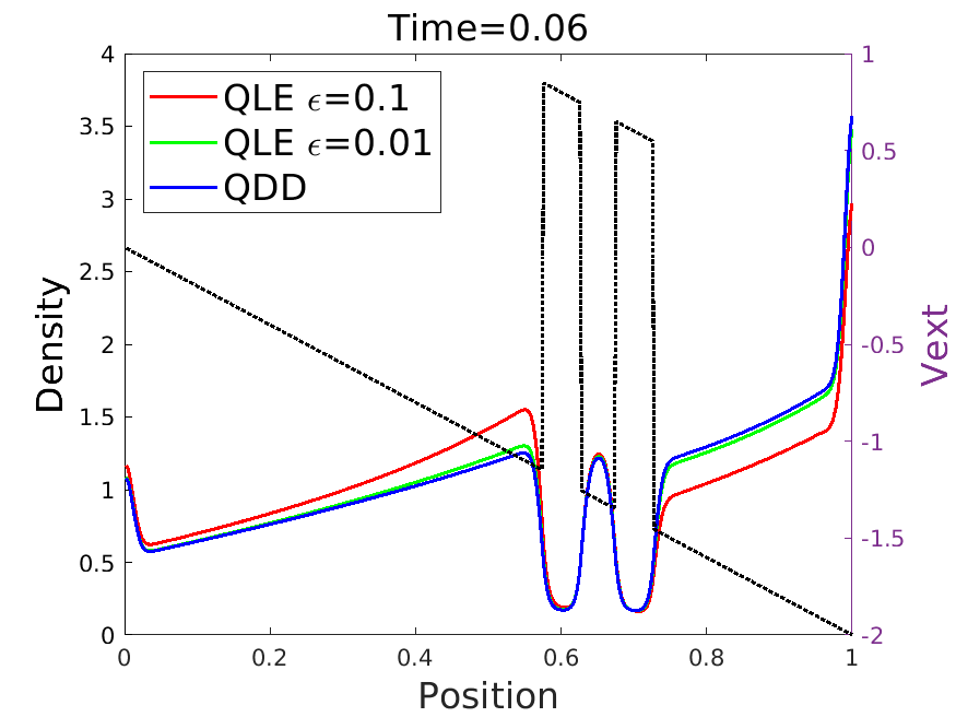
We compare in this section the solutions to QDD and to QLE for various values of . We will see that the models agree when is sufficiently small, which is the regime of validity of QDD. We consider three situations: (i) in the first one, the initial condition is well-prepared in the sense that it is a quantum Maxwellian associated with a given Hamiltonian. This prevents the creation of initial layers as is customary in diffusion limits. We then switch at the initial time the potential in this Hamiltonian and observe how the system converges to a new equilibrium. (ii) The situation in the second case is slightly less favorable in the sense that the initial density operator is function of an Hamiltonian, but not a quantum Maxwellian. (iii) In the last scenario, we consider an ill-prepared initial condition that is a combination of wave packets; in this case, there is an initial layer and in order to minimize its effects and observe good agreement between QLE and QDD for earlier times, the parameter has to be decreased ( in the last case versus in the first two).
In all simulations, we set the tolerance for the nonlinear conjugate gradient and the associated line search to . The number of spatial discretization points is . The parameter is set to for simplicity, which is of the order of magnitude of values found for semiconductor devices such as the resonant tunneling diode, for which [5]. As already mentioned, is small in interesting regimes, and we set for instance .
In all density operators, we discard the modes associated with weights (i.e. eigenvalues) less than . This leaves approximately between 50 and 100 modes in the quantum Maxwellian for instance, and improves computational time. With , and considering the quantum Maxwellian with the free Neumann Hamiltonian, we have about 50 modes with weights greater than , and about 30 others with weights between and .
Quantum Maxwellian.
We set for initial condition
where is the double barrier potential shown in figure 2, top left panel (the width of the well and the barriers is 0.05, with height equal to 2). Such a potential is characteristics of the resonant tunneling diode, see [5] and references therein. The density associated to is depicted in the same panel. At time , the potential is switched to , which is now the exterior potential used in the resolution of QLE and QDD and promotes particle transport from left to right. It is depicted in the other panels of figure 2. The time stepsize is set to for the calculations.
We then represent in figure 2 the transition to the new equilibrium associated to , from time to (which is close to the time at which the equilibrium is reached by QDD). We observe a remarkable agreement between QDD and QLE with , with an overall space-time relative error of about . When , the diffusive regime is not valid and as a consequence QLE and QDD produce different densities.
Function of an Hamiltonian.
We set
with and the same parameters as in the previous paragraph. The situation is very similar as above with a very good agreement between QDD and QLE with and an error again of the order of . The densities are depicted in figure 3.
Superposition of wave packets.
We set
where is the function , and is the density operator
where and . The associated density is represented in the top left panel of figure 4, along with the (fixed this time) double barrier potential used in the calculations. In the localizing function , we choose and . The parameter acts as a regularization since the gaussian function is very small away from its center. Small densities create large chemical potentials which generate numerical instabilities, and we found that such an improves the convergence of the minimization algorithms.
The simulations, represented in figure 4, show that is far too large to capture the diffusive regime. When , the comparison improves with a space-time relative error of about . In order to observe a very good agreement, we decrease to . For the simulations with , the time stepsize is set at to obtain sufficient accuracy. This substantially increases the numerical cost and makes the numerical method not effective for such small values of . The relative error between QDD and QLE with is now of order . One would need to resort to asymptotic preserving schemes to capture the regime at an affordable cost, see e.g. [18, 22].




6 Conclusion
We have introduced in this work a time-splitting scheme for the resolution of the quantum Liouville-BGK equation. The splitting allows us, exploiting the local conservation of particles, to obtain a completely linear collision step. The minimization problem involved in the latter is solved by using the nonlinear conjugate gradient algorithm, and good initial guesses can be obtained by taking advantage of some small parameters. We applied our numerical method for comparing the solutions to the quantum Liouville-BGK equation and to the quantum drift-diffusion, and obtained excellent agreement in the regime of validity of the latter.
An important limitation of the method is the requirement that the time stepsize be small compared to the rescaled mean free path for good accuracy. We plan in the future on removing this restriction by designing an asymptotic preserving scheme in the spirit of [18, 22]. This would allow us to capture the correct solution for arbitrarily small values of at a reasonable computational cost.
Appendix A Appendix
A.1 Derivation of the 1D model
We derive in this section a 1D model as a simplification of a 3D model. We consider a 3D domain of the form , where is periodic as explained in the introduction, and we choose the 2-torus for simplicity. We then write
| (22) |
in the sense that the two spaces are unitarily equivalent, and the 3D Hamiltonian is expressed as
where (all physical constants are set to one),
and denotes, with an abuse of notation, the identity operator in both and . Above, is a given bounded potential. The operator is equipped with the domain defined in (3), and with the domain consisting of periodic functions. The 3D Liouville-BGK equation is then
| (23) |
where is the unique minimizer of the 3D free energy
under the constraint that . We set , so that for all . Note that the traces above are taken w.r.t. , and that we removed linear term in the entropy since it is fixed to one by the constraint. Let
where denotes trace w.r.t. . It is clear that is the unique minimizer of the “transverse” free energy
under the constraint that . The free energy is indeed, up to a constant term, equal to the relative entropy between and and which vanishes when . Above, is the transverse entropy
We will show that if the initial condition has the tensor form ( acts on the space ), namely that the initial state of the system is at equilibrium in the transverse plane, then the solution remains in a similar form and reads . While it is direct to separate variables in , it has to be proved that the minimizer for also admits a tensor form . This is a consequence of (22) and of the subaddivity of the von Neumann entropy . More precisely, we have the following lemma:
Lemma A.1
Let , with . Then, the unique minimizer of with constraint has the form
where is the minimizer of the 1D problem with constraint .
The 1D problem mentioned in the lemma consists in minimizing the 1D free energy
under the constraint that . Above, is the “longitudinal” entropy
where denotes trace w.r.t. .
Proof. That admits a unique minimizer was established in [26] under appropriate conditions on the constraint . Furthermore, with the notations
for the partial traces w.r.t. and , respectively, and for any density operator on , the subaddivity of yields, see [1],
Hence, for any density operator on with ,
Above, denotes for simplicity, and we used that implies . Finally, since a direct calculation shows that , it follows that for any density operator satisfying the constraint . Since the eigenfunctions of are complex exponentials as a consequence of the periodic boundary conditions, it follows that , and therefore that . Hence, is the unique minimizer of under the local constraint .
We are now in position to conclude. We need the following assumptions on the solutions to (23): we suppose that (i) (23) admits a unique solution under appropriate conditions on the initial condition , and (ii) that this solution is obtained as the limit in proper sense as of the sequence , that satisfies the linear problem
| (24) |
Items (i) and (ii) are established in 1D in [27] without the uniqueness result, the latter being proven in Section 3.2 in the present paper. The 3D case is still open.
We proceed by induction to obtain that where verifies
For , we have with , and therefore, according to Lemma A.1, . Since (24) is linear and admits a unique solution, it follows that for an appropriate . Since the same reasoning applies for any , we obtain that . Using assumption (ii), it follows that the 3D solution reads , where verifies the 1D equation
Note that we considered a linear potential in this section, but the same approach holds for the 3D Poisson potential since the resolution of the Laplace equation with Dirichlet boundary conditions on and periodic on yields .
This ends the justification of the 1D model.
A.2 Proof of Lemma 3.2
Given , we recall that one iteration of the splitting scheme reads
where , and is the solution to
| (25) |
Existence and uniqueness.
We show first that the above is well-defined and unique. We proceed iteratively. First, if is a density operator in , then so is for all since preserves self-adjointness and positivity, and
Let . Considering the collision subproblem , we recall that (25) preserves the local density, and a consequence the equation is linear and admits as solution
| (26) |
provided exists and is unique. According to [25, Theorem 2.1], the latter holds when , and when for all , yielding a unique . We already know that from the previous step, and need to prove the lower bound. Following the assumptions of Theorem 3.1, for any ,
and, under again the assumptions of Theorem 3.1, we have
This shows that for all , and therefore that exists in and is unique. Hence, is well-defined, and as a consequence so is in . We now iterate over . Since is nonnegative, we have from (26), for all ,
which allows us to construct and therefore . Iterating, we then find and, from the version of (26) at step ,
| (27) |
which proves the lower bound on for all and all . We have therefore obtained a unique solution to the splitting scheme in satisfying the lower bound announced in the lemma.
Uniform bounds.
We derive now a bound in that is uniform in and . For this, we need first uniform bounds in and in . The one in is direct as is an isometry in and (25) preserves trace, and therefore
For the bound in , we remark that is an isometry in , and that we have the following bound from Proposition 2.2 in [27]:
where is independent of . With the above definition of , this yields,
since for . Going back to the splitting solution , we therefore obtain
Iterating, it follows that
which provides us with a uniform bound in . We move on now to the bound, and use the following result from [27]: let , with and . Then,
| (28) |
With the above definition of , this yields
where the constant is independent of and since the lower bound in (27) and the bound in are uniform in and . Going back to the splitting solution , we therefore obtain
Iterating, it follows that
This ends the proof.
A.3 Proof of Lemma 3.3
Before proceeding with the proof, the following generalized Gronwall Lemma will be useful. The proof of the general result can be found in [4].
Lemma A.2 (Gronwall)
Let be continuous and satisfy the inequality,
where . Then, the following estimate holds
where and .
The following two Lemmas can be found in [27] and will be used in the proof.
Lemma A.3 (Lemma 6.4 in [27])
Let , self-adjoint and nonnegative. Then,
The result below shows that the map is at least of Hölder regularity in .
Lemma A.4 (Corollary 5.8 in [27])
Let and be two density operators in . Let be such that
Then,
where is independent of and .
We can now proceed with the proof. According to (11) and (12), the error for , with the notation , verifies
where and . Taking the norm and using the fact that is an isometry on , we find for ,
First, consider the integral given by . We have, since is an isometry on ,
The first inequality is thanks to Lemma A.3 and the fact that . The second inequality is due to the sublinear estimate stated in (28), which holds provided and is bounded uniformly in . These two facts are obtained in Lemma 3.2 as . The last inequality is due to estimate (13) in Lemma 3.2.
Now, consider the integral term . We apply Lemma A.4 as both and belong to and their respective local densities are uniformly bounded from below according to Theorem 3.1 and Lemma 3.2. Then, with ,
The term will be handled further with the Gronwall Lemma. For , we remark first that from (11) and Lemma 3.2,
Then, using again Lemma 3.2 and Lemma A.3, we find, for ,
Collecting all estimates, we have for ,
The generalized Gronwall Lemma then yields, using that for and , for ,
This ends the proof.
A.4 Semi-classical approximation
We obtain relation (21) by using pseudo-differential calculus, and need for this to extend the problem to the whole . We remain at a formal level. Let then be a smooth function over such that , with for , and for , for some . Denoting by quantities that are negligible in appropriate sense when , we have, for any smooth function ,
| (29) |
since the size of the support of is less than . Next, we remark that the function is equal to the function , with solution to
Consider then the operator defined on , with on and for . With , we find that
where
and the hypotheses on yield . This shows that
and as a consequence, with (29),
| (30) |
We are now in position to use pseudo-differental calculus and find an approximation for , which is well-defined since is trace class because of the confining potential . It is shown in [9] that
and therefore, according to (30),
This gives (21). Regarding the approximate functional, we set and find
The functional is finally obtained by spatial discretization. This ends this section.
References
- [1] H. Araki and E. Lieb. Entropy inequalities. Communications in Mathematical Physics, 18(2):160 – 170, 1970.
- [2] A Arnold. Numerical absorbing boundary conditions for quantum evolution equation. VLSI Design, 6:313–328, 1998.
- [3] P. Bhatnagar, E. Gross, and M. Krook. A model for collision processes in gases .1. Small amplitude processes in charged and neutral ibe-component systems. Physical Review, 94(3):511–525, 1954.
- [4] I. Bihari. A generalisation of a lemma of Bellman and its application to uniqueness problems of differential equations. Acta Math. Acad. Sci. Hungarica, 7:81–94, 1956.
- [5] P. Degond, S. Gallego, and F. Méhats. An entropic quantum drift-diffusion model for electron transport in resonant tunneling diodes. Journal of Computational Physics, 221(1):226–249, 2007.
- [6] P. Degond, S. Gallego, and F. Méhats. Isothermal quantum hydrodynamics: derivation, asymptotic analysis, and simulation. Multiscale Model. Simul., 6(1):246–272, 2007.
- [7] P. Degond, S. Gallego, and F. Méhats. On quantum hydrodynamic and quantum energy transport models. Commun. Math. Sci., 5(4):887–908, 2007.
- [8] P. Degond, S. Gallego, F. Méhats, and C. Ringhofer. Quantum hydrodynamic and diffusion models derived from the entropy principle. In Quantum transport, volume 1946 of Lecture Notes in Math., pages 111–168. Springer, Berlin, 2008.
- [9] P. Degond, F. Méhats, and C. Ringhofer. Quantum energy-transport and drift-diffusion models. J. Stat. Phys., 118(3-4):625–667, 2005.
- [10] P. Degond, F. Méhats, and C. Ringhofer. Quantum hydrodynamic models derived from the entropy principle. In Nonlinear partial differential equations and related analysis, volume 371 of Contemp. Math., pages 107–131. Amer. Math. Soc., Providence, RI, 2005.
- [11] P. Degond and C. Ringhofer. Quantum moment hydrodynamics and the entropy principle. J. Statist. Phys., 112(3-4):587–628, 2003.
- [12] R. Duboscq and O. Pinaud. A constrained optimization problem in quantum statistical physics. Submitted.
- [13] R. Duboscq and O. Pinaud. Entropy minimization for many-body quantum systems. Submitted.
- [14] R. Duboscq and O. Pinaud. On local quantum gibbs states. Submitted.
- [15] R. Duboscq and O. Pinaud. On the minimization of quantum entropies under local constraints. Journal de Mathématiques Pures et Appliquées, 128:87–118, 2019.
- [16] R. Duboscq and O. Pinaud. Constrained minimizers of the von Neumann entropy and their characterization. Calculus of Variations and PDEs, 59(105), 2020.
- [17] S. Gallego and F. Méhats. Entropic discretization of a quantum drift-diffusion model. SIAM J. Numer. Anal., 43(5):1828–1849, 2005.
- [18] S. Jin. Asymptotic preserving (AP) schemes for multiscale kinetic and hyperbolic equations: a review. Rivista di Matematica della Università di Parma. New Series, 2, 01 2010.
- [19] A. Jüngel. Quasi-hydrodynamic semiconductor equations. Progress in Nonlinear Differential Equations and their Applications, 41. Birkhäuser Verlag, Basel, 2001.
- [20] A. Jüngel and D. Matthes. A derivation of the isothermal quantum hydrodynamic equations using entropy minimization. ZAMM Z. Angew. Math. Mech., 85(11):806–814, 2005.
- [21] A. Jüngel, D. Matthes, and J. P. Milišić. Derivation of new quantum hydrodynamic equations using entropy minimization. SIAM J. Appl. Math., 67(1):46–68, 2006.
- [22] M. Lemou and L. Mieussens. A new asymptotic preserving scheme based on micro-macro formulation for linear kinetic equations in the diffusion limit. SIAM Journal on Scientific Computing, 31(1):334–368, 2008.
- [23] C. D. Levermore. Moment closure hierarchies for kinetic theories. J. Statist. Phys., 83(5-6):1021–1065, 1996.
- [24] P.-L. Lions and T. Paul. Sur les mesures de Wigner. Rev. Mat. Iberoamericana, 9:553–618, 1993.
- [25] F. Méhats and O. Pinaud. An inverse problem in quantum statistical physics. J. Stat. Phys., 140(3):565–602, 2010.
- [26] F. Méhats and O. Pinaud. A problem of moment realizability in quantum statistical physics. Kinet. Relat. Models, 4(4):1143–1158, 2011.
- [27] F. Méhats and O. Pinaud. The quantum Liouville-BGK equation and the moment problem. J. of. Diff. Eq., 263(7):3737–3787, 2017.
- [28] B. Nachtergaele and H-T. Yau. Derivation of the Euler equations from quantum dynamics. Comm. Math. Phys., 243(3):485–540, 2003.
- [29] O. Pinaud. Transient simulations of a resonant tunneling diode. J. App. Phys., 92:1987–1994, 2002.
- [30] O. Pinaud. The quantum drift-diffusion model: existence and exponential convergence to the equilibrium. Annales de l’Institut Henri Poincaré C, Analyse non linéaire, 36(3):811–836, 2019.