A phase field model for mass transport with semi-permeable interfaces
Yuzhe Qin
Affiliation: Research Center for Mathematics,
Beijing Normal University at Zhuhai, 519087, China
Affiliation: Research Center for Mathematics and Mathematics Education,
Beijing Normal University at Zhuhai, 519087, China
Affiliation: Laboratory of Mathematics and Complex Systems (Ministry of Education),
School of Mathematical Sciences,
Beijing Normal University, Beijing 100875, China
Huaxiong Huang
Affiliation: BNU-UIC Joint Mathematical Research center,
Beijing Normal University, Zhuhai 519087, China
Affiliation: Department of Mathematics and Statistics, York University,
Toronto, Ontario, Canada
Affiliation: Corresponding authors, Shixin.xu@dukekunshan.edu.cn; hhuang@uic.edu.cn
Yi Zhu
Affiliation: Department of Mathematics and Statistics, York University,
Toronto, Ontario, Canada
Chun Liu
Affiliation: Department of Applied Mathematics, Illinois Institute of Technology, IL 60616, USA
Shixin Xu
Affiliation: Duke Kunshan University, 8 Duke Ave, Kunshan, Jiangsu, China
Affiliation: Corresponding authors, Shixin.xu@dukekunshan.edu.cn; hhuang@uic.edu.cn
Abstract
In this paper, a thermal-dynamical consistent model for mass transfer across permeable moving interfaces is proposed by using energy variation method. We consider a restricted diffusion problem where the flux across the interface depends on its conductance and the difference of the concentration on each side. The diffusive interface phase-field framework used in here has several advantages over the sharp interface method. First of all, explicit tracking of the interface is no longer necessary. Secondly, the interfacial condition can be incorporated with a variable diffusion coefficient. A detailed asymptotic analysis confirms the diffusive interface model converges to the existing sharp interface model as the interface thickness goes to zero. A
decoupled energy stable numerical scheme is developed to solve this system efficiently. Numerical simulations first illustrate the consistency of theoretical results on the sharp interface limit. Then a convergence study and energy decay test are conducted to ensure the efficiency and stability of the numerical scheme. To illustrate the effectiveness of our phase-field approach, several examples are provided, including a study of a two-phase mass transfer problem where drops with deformable interfaces are suspended in a moving fluid.
1 Introduction
Mass transfer through a semi-permeable or conducting interface
is a common phenomenon in biology [12, 9] and material science [8, 13].
A representative example is that cell membranes are permeable to oxygen [26], ATP [33] and ions [17].
In this case, the domain consists of intracellular space denoted by and extracellular space denoted by with a cell membrane in between (see Figure 1 ).
Figure 1: Schematic of mass transport across the membrane.
The diffusion of concentration can be described by the following diffusion equation in the bulk [30],
(1.1)
where represent the concentration of the molecule and velocity of fluid in and is the diffusion coefficient in . Here may be discontinuous cross the boundary, like the ion concentrations in [23].
At the interface , the trans-membrane flux is set to be continuous
(1.2)
where is the permeability, denotes the jump of concentration across the interface and
is the unit normal vector of the interface. Here could have different formats, like in [9] or in [30].
There are numerous papers investigating for mass transfer.
As a matter of fact, the mass transfer phenomenon can be attributed to diffusive process in binary flows involving free boundaries.
For the standard fluid-structure interaction problems, a variety of methods are developed over the past decades. There are two most popular classes of technique, the sharp interface methods, like level set methods [1], immerse boundary methods [18], immerse interface methods [15], front tracking methods [24], and diffuse interface methods [32]. For mass-transfer across liquid–gas interface, volume of fluid methods are proposed to solve the phase change problem [27, 6] and bubble
behaviours with water system [16]. The immersed interface method is extended to study water transport accross a deformable membrane by Layton [14].
The immerse boundary method, due to its simplicity, has been applied to many fluid flow problems and has become one of the main numerical techniques for scientific computation.
Gong and Huang et al. [9, 26] developed a series of work to understand oxygen transport across permeable membrane by using immerse interface method. In order to ensure the restrict diffusion on the membrane (1.2), an additional equation is introduced to describe the temporal evolution of diffusive flux.
Unlike sharp interface methods, where the interface are handled separately by using function or local reconstruction, the diffusive interface method models the two phase flow and the interface in a uniform way by a label function
[3, 2, 4].
The basic idea can be dated back to van der Waals in the late 19th century[25]. The main advantage of diffusive interface method is that follows the energy dissipation law such that the obtained model is thermal-dynamical consistent. It makes it possible to design efficient energy stable schemes for long time simulation. However, to our best knowledge, there is not a diffusive interface model for mass transport through a semi-permeable membrane. The main challenge is how to impose the restricted diffusion near interface such that as interface thickness goes to zero, the sharp interface limit is consistent with boundary condition (1.2).
In this paper, a thermal-dynamical consistent diffusive model is first proposed by using energy variational method [22], which starts from two functionals for the total energy and dissipation, together with the kinematic equations based on physical laws of conservation.
The key is to modify the diffusion coefficient as a function of and interface permeability . The restricted diffusion only means that the changing rate of energy near the interface follows a specific dissipation rate functional. Then following the results of Xu et al. [31], a detailed asymptotic analysis is presented to confirm the proposed diffusive interface model converges to the existing sharp interface model (1.1) and (1.2) as the interface thickness goes to zero. In the next, based on the energy dissipation law, an efficient energy stable decoupled scheme is proposed to solve the obtained system.
The structure of the paper is as follows.
In section 2, the phase field model for mass transport through a semi-permable interface is proposed by using energy variational method.
In section 3, the sharp interface limits of the phase field model are presented
by asymptotic analysis.
A decoupled, linear and unconditional energy stable numerical
scheme is developed in section 4 by means of the stabilization method and pressure correction method.
In section 5, numerical experiments are carried out to verify our theoretically
results and study the membrane permeability effect.
Finally, conclusions are drawn in section 6.
2 Phase field model for mass transfer with hydrodynamics
In this section, energy variation method is used to derive a diffusive interface model for mass transport through a semi-permeable membrane with restrict diffusion.
2.1 Model derivation
First, phase field variable is introduced to label the different domain,
(2.1)
The interface between the two domains is described by the zero level set
.
We will omit the subscript in the following, i.e.
we use to instead .
We start from the following kinematic assumptions on the laws of conservation: in domain
(2.2a)
(2.2b)
(2.2c)
(2.2d)
where is the density, is the phase label function, is the concentration of a substance, is the fluid velocity, and is the material derivative.
Here Eq. (2.2a) is the conservation of label function with unknown flux ; Eq. (2.2b) is the conservation of mass with unknown mass flux ; Eq. (2.2c) is the conservation of momentum with unknown stress induced by viscosity of fluid
and stress induced by two-phase flow interface .
On the boundary of the domain, the boundary conditions can be given as
(2.3)
where is the outward normal on the domain boundary .
Then the system (2.2) conserves the local mass density,
i.e.
and .
The total energy consists of kinetic energy, mix entropy and the phase mixing energy
(2.4)
where is the double well potential.
is the gas constant number, is the thermodynamic temperature,
is the reference concentration,
is the energy density, is the thickness of the interface.
Then according to the total energy, we could define the chemical potentials
(2.5)
(2.6)
The dissipative functional is composed of the dissipation due to fluid friction, irreversible mixing of the substance and irreversible mixing of two phases in bulk
(2.7)
where is the viscosity for the fluid,
is the strain rate, is the phenomenological mobility.
In order to model the restricted diffusion due to the permeability of the interface, the diffusion coefficient is modelled in the following way
(2.8)
where is the permeability for the membrane, is a constant to be determined, and
and are the diffusion coefficients in domain
and
respectively.
The energy dissipative law [7, 30, 22] states that without external force acting on the system, the changing rate of total energy equals the dissipation
(2.9)
Then the definition of total energy functional (2.4) yields
(2.10)
By using the definitions of chemical potential (2.5) and conservation law (2.2b), the first part yields
(2.11)
where the nonflux boundary condition for is used here.
For the second term, by using Eqs.(2.2c) and (2.2d), we have
(2.12)
where pressure is induced as a Lagrange multiplier for incompressibility.
The last term is calculated with Eqs(2.2a) and (2.6)
(2.13)
where the nonflux boundary of is used.
Then substituting above three equations to Eq. (2.10) yields
(2.14)
Comparing two sides of the above equation (2.1)
and calculating the functional deriative, we obtain
(2.15a)
(2.15b)
(2.15c)
(2.15d)
Then the diffusive interface model for mass transport through semi-permeable membrane with restricted diffusion is summarized as follows
(2.16a)
(2.16b)
(2.16c)
(2.16d)
(2.16e)
(2.16f)
(2.16g)
with boundary conditions
(2.17)
2.2 Non-dimensionalization
Now we introduce the dimensionless variables
(2.18)
Here are the characteristic length, time, concentration velocity and diffusion constant.
For convenience, the tilde symbol will be removed in the dimensionless quantities, and the dimensionless system of (2.16) is given by
(2.19a)
(2.19b)
(2.19c)
(2.19d)
(2.19e)
(2.19f)
(2.19g)
with the boundary condition
(2.20)
with the dimensionless parameters
(2.21)
Remark 2.1.
During the dimensionless, we use the fact that
and redefine pressure function
Theorem 2.1.
If , , and are smooth solutions of the system (2.19)
with boundary condition (2.20), then the following energy law is satisfied:
(2.22)
where
(2.23)
Proof.
By taking the inner product of (2.19a), (2.19c), (2.19d),
(2.19e) and (2.19f) with , , ,
and respectively, one obtains immediately (2.22).
∎
3 Sharp interface limit
In this section, a detailed asymptotic analysis is presented by using the results in [31] to show the sharp interface limits of the obtained system (2.19). Here we assume the viscosity is constant and , where is a constant independent of .
3.1 Outer expansions
Far from the two-phase interface , we use the following ansatz:
(3.1a)
(3.1b)
(3.1c)
(3.1d)
(3.1e)
(3.1f)
Sine the concentration does not effect equations of and , we directly call the results in [31],
(3.2a)
(3.2b)
(3.2c)
(3.2d)
Substituting (3.1e),(3.1f)
into Eq. (2.19e) yields
we have
We first introduce the signed distance function to the interface .
Immediately, we have .
After defining a new rescaled variable
(3.7)
for any scalar function , we can rewrite it as
(3.8)
and the relevant operators are
(3.9a)
(3.9b)
(3.9c)
and for a vector function , we have
(3.10)
Here the and stand for the gradient and Laplace
with respect to , respectively.
And we use the fact that .
for is
the mean curvature of the interface.
In the inner region, we assume that
Combining the above analysis, at the leading order, we obtain the following results:
(3.26a)
(3.26b)
(3.26c)
(3.26d)
(3.26e)
(3.26f)
(3.26g)
This illustrates that our diffusive interface model converges to the sharp interface model for mass transport with constrict diffusion condition (2.15b).
4 Numerical Method
The system (2.19) is a totally nonlinearly coupled model.
In this section, we focus on developing an unconditionally energy stable numerical scheme
for our proposed mathematical model based on the stabilization method
[29, 20, 34, 21, 19].
In order to assure the conservation of volume of the numerical scheme, we need to rewrite some terms of system (2.19),
taking into account the following relations:
(4.1)
Then, we redefine the pressure therm as
(4.2)
For simplicity of notation, we rewrite instead of .
Given initial conditions , , , and ,
we compute (, , , , , )
for by the following steps.
Step 1. We solve phase field variable by the following scheme with the help of
Stabilization method and Navier-Stokes equation by pressure correction method
[5, 10]:
(4.3a)
(4.3b)
(4.3c)
with the boundary condition
(4.4)
Step 2. Projection step:
(4.5a)
(4.5b)
with boundary condition
(4.6)
Step 3. will be updated by the following fully implicit Euler scheme:
(4.7a)
(4.7b)
(4.7c)
(4.7d)
with boundary condtion
(4.8)
Theorem 4.1.
System is uniquely solvable,
unconditionally stable and obey the following discrete energy law:
(4.9)
where denotes the discrete norm in domain .
Remark 4.1.
Numerical scheme (4.3) is a coupled system for and
. Block Gauss iteration method is used to compute this system efficiently.
5 Numerical results
In this section, some numerical experiments are conducted to illustrate validity of our model.
We first check the sharp interface limit results in Section 3 by choosing smaller and comparing with analytical solutions of sharp interface models. Then we check the convergence rate and energy stability of the numerical scheme in Section 4. Finally, the calibrated model and scheme are used to study the effect of interface permeability.
Block-centered finite difference method based on stagger mesh is adopted to discretize equations
(2.19) in space.
Variables , and are located in the center of mesh,
however velocity variables and are located on the center of edge.
The main advantage of the block-centered finite difference method is
it approximates the phase function, concentration function and pressure function with
Neumann boundary condition to second-order accuracy, and also, it guarantees local mass conservation.
5.1 Sharp interface limit test
In this example, we take the steady state in 1D case to verify sharp interface limit of
concentration function . For simplicity, we first fixed the interface and only solve concentration equation (2.19e) where interface is assumed at in domain .
The diffusion coefficient is taken as and
Dirichlet boundary condition is used.
Then in this case, the exact solution of sharp interface model (1.1)-(1.2) is
(5.1)
In Figure 2, the exact solution of is shown in black solid line and the dash lines are the solutions of Eq. (2.19e) where the phase field function is chosen as
with different interface thickness . In the bulk region, solutions of two methods fit very well.
As , the proposed diffusive model solutions change much sharper near the interface and convergence to the sharp interface solution, which is consistent with our analysis in Section 5.3.1.
Figure 2: Sharp interface limit
5.2 Comparison with sharp interface model
In this subsection, we conduct two numerical tests to compare with the results using immersed boundary methods [11].
The first experiment is 1D steady state solution of Eqs. (1.1)-(1.2)
with , . The locations of interfaces are chosen at and , i.e. and and diffusion constants are . In this case, the exact solution can be obtained as
(5.2)
In Figure 3, the solid black line is above exact solution, blue line with circle is the immerse boundary method solution and the red line with square is the the diffusive interface solution with interface width .
We can see that the numerical solution is almost coincided with the exact solution and
there is indistinguishable difference between our results and the immerse boundary result in [11].
Figure 3: Steady state solution with the linear law on the interfaces located at
and with , , and . The black solid line is the exact solution,
and the red dash with square is the numerical solution by phase field method,
but the blue dash with circle is the numerical solution by immersed boundary method.
In the next, the 2D validation is conducted where the interface is fixed as a circle with radius and center at .
The initial condition of concentration (see Fig. 4 (a)) and parameters
are set to be same as those in [11],
, where
(5.3)
with
(5.4)
The computational domain is discretized by a uniform grid with size and interface thickness .
Fig.4 (b) show the distribution of concentrations by using immerse boundary method (dash lines) [11] and proposed diffusive interface method (solid lines) at time .
It illustrates that our diffusive interface model fits the immerse interface results very well for the concentration through the semi-permeable interface with restrict diffusion.
(a)Initial condition of concentration.
(b)Snapshot of level curves of concentration at .
Figure 4: Comparison between phase field method and immersed boundary method for mass transfer. The fixed interface is expressed with bold cure marked by 0.
(a): The initial condition of concentration that concentrates in the centre. (b): Snapshot of level curves of concentration by using different methods.
The dashed lines are level curves obtained by immersed boundary method [11] and the solid lines are the level curves obtained by proposed diffusive interface method.
5.3 Convergence study and unconditional energy stability
In this section, we conduct the convergence test and unconditional energy stable test to
illustrate the effectiveness of our proposed numerical scheme.
Here we use the uniform mesh, namely we use the mesh size , and if not specified,
uniform mesh is always tenable.
5.3.1 Convergence rate test
In this subsection, we perform some numerical experiments to support the theoretical results.
We use a uniform Cartesian grid to discretize a square domain .
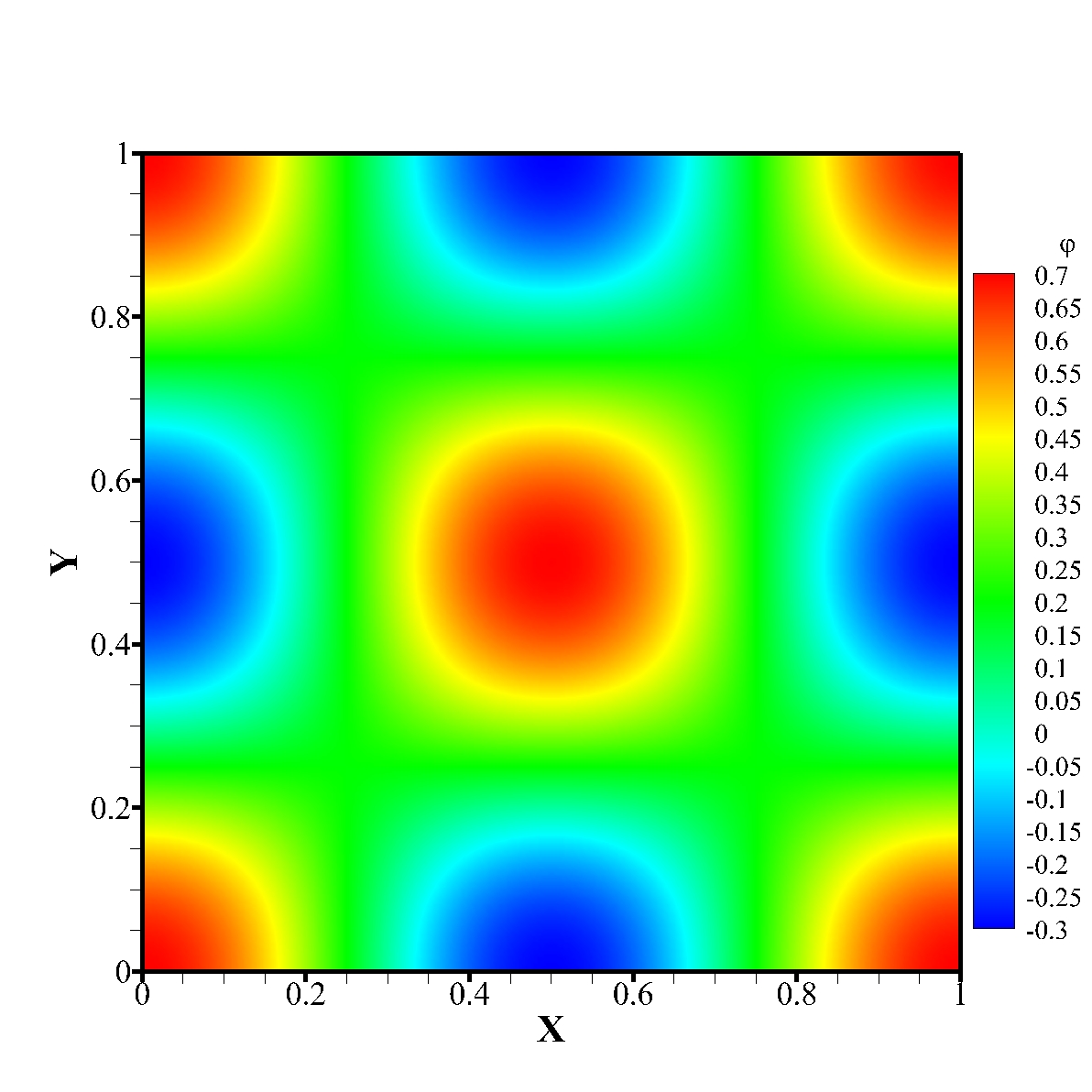
The initial condition is chosen as follows, ( see Fig. 5)
(5.5a)
(5.5b)
(5.5c)
(5.5d)
Periodic boundary conditions are adopted for all variables.
The parameters in model (2.19) are set as
(5.6)
(a).
(b).
Figure 5: Initial conditions for convergence study. (a): concentration ; (b): phase field function . 5.5.
The Cauchy error [28] is used to test the convergence rate.
In this test method, error between two different spacial mesh sizes and is calculated by
, where is the function to be solved. The mesh sizes are set to be
and time step is fixed as .
The and numerical errors and convergence rate at chosen time are displayed in Table
1 and Table 2, respectively.
The second order spatial accuracy is apparently observed for all the variables.
Table 1: The discrete error and convergence rate at
with initial data (5.5) and the given parameters.
Grid sizes
Error
Rate
Error
Rate
Error
Rate
Error
Rate
Error
Rate
4.01e-02
–
1.01e-02
–
1.15e-04
–
1.15e-04
–
1.57e-03
–
8.90e-03
2.17
4.91e-03
1.90
3.23e-05
1.83
3.23e-05
1.83
1.24e-04
3.66
2.22e-03
2.01
6.80e-04
1.99
8.06e-06
2.00
8.06e-06
2.00
3.00e-05
2.05
5.54e-04
2.00
1.70e-04
2.00
2.01e-06
2.00
2.01e-06
2.00
7.46e-06
2.01
1.38e-04
2.00
4.26e-05
2.00
5.04e-07
2.00
5.04e-07
2.00
1.86e-06
2.00
Table 2: The discrete error and convergence rate at
with initial data (5.5) and the given parameters.
Grid sizes
Error
Rate
Error
Rate
Error
Rate
Error
Rate
Error
Rate
7.64e-02
–
1.89e-02
–
1.83e-04
–
1.83e-04
–
3.99e-03
–
1.69e-02
2.17
4.91e-03
1.95
5.00e-05
1.88
5.00e-05
1.88
2.53e-04
3.98
4.18e-03
2.02
1.23e-03
1.99
1.25e-05
2.00
1.25e-05
2.00
5.89e-05
2.10
1.03e-03
2.02
3.07e-04
2.01
3.12e-06
2.00
3.12e-06
2.00
1.50e-05
1.98
2.55e-04
2.01
7.61e-05
2.01
7.80e-07
2.00
7.80e-07
2.00
3.71e-06
2.01
5.3.2 Unconditionally energy stable test
In this subsection, we carry out a numerical experiment to survey the unconditionally energy
stability about our numerical scheme with the same initial condition and boundary conditions.
The result is listed in Figure 6.
Time steps are chosen from to with fixed spacial mesh size .
The total energy dynamics over time with different time steps are shown in Fig. 6. It illustrates that the energy is monotonic decrease with different time steps which confirms the unconditional energy stability of the proposed scheme.
Figure 6: Unconditional energy stability with different time steps represented by
different markers and colors.
We utilize the result computed with time step to give the conservation of volume about our numerical scheme for as illustrated in Fig. 7.
It demonstrates the volume of doesn’t change over time.
Figure 7: Conservation of volume of the numerical scheme with time step .
5.4 Effect of interface permeability
In this subsection, the calibrated model and scheme are used to study the effect of interface permeability on the diffusion of substance concentration.
We first consider a single drop with high (), medium () and low (() permeability with , is suspended in a shear flow.
The initial profiles of concentration and interface are given as follows (see Fig. 8),
(5.7a)
(5.7b)
with boundary condition
and periodic boundary conditions are used on the left and right boundaries.
The parameters read as
(5.8)
(a)Initial condition of .
(b)Initial condition of .
Figure 8: Initial condition for example 5.7.
We set the concentration is a linear function with y-direction.
The phase field function is a circle with a diffuse interface.
The velocity is a shear flow.
The 2D and 3D profiles of concentration at steady states are shown in Figs. 9-10. When the interface with large permeability, the distribution of concentration is close to the linear solution where no interface is presented. This could also be observed by the direction of flux in Fig. 11 (a) and magnitude of flux in Fig. 12(a).
When the permeability decreases, the flux across the interface decreases (see Fig. 12(b-c)), and are close to nonflux boundary condition such that the straight flux is disturbed around the boundary as shown in Fig. 11(b-c) and trans-membrane flux is restricted.
At the steady state, due to limited flux on the interface, the inner region is almost a constant (see Figs. 9-10 (c)) due to the diffusion inside and very limit flux , while the profile of concentration in the out region is close to the diffusion in a perforated domain.
(a) Higher permeability
(b)Medium permeability
(c)Lower permeability
Figure 9: Snapshots of at steady state with different permeability: and .
(a)Higher permeability
(b)Medium permeability
(c)Lower permeability
Figure 10: 3D profile of at steady state with different permeabilities
and .
(a)Higher permeability
(b)Medium permeability
(c)Lower permeability
Figure 11: Snapshot of the magnitude for flux at steady state with different permeabilities
and .
(a)Higher permeability
(b)Medium permeability
(c)Lower permeability
Figure 12: Snapshot of the magnitude for flux at steady state with different permeabilities
and
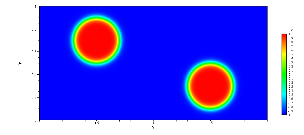
In the next, we consider there are two droplets in the shear flow in a rectangular area .
The initial condition for is considered as
(5.9)
The permeability is chosen as .
The initial conditions of and and all the parameters are chosen the same as in the former example (5.7).
As shown in Fig. 13, the initial profiles of concentration and
droplets are shown in Fig. 13
(a).
(b).
Figure 13: Profile of initial condition.
In Fig. 14, the magnitude of flux overtime are presented. Due the counter flow, two droplets move closer and the merge into one droplet around time . Before , the restrict diffusion are observed on two interface and the concentrations in two droplets are two distinct constants as shown in Fig. 15 a-b. After the merge time, the droplet achieves new equilibrium of concentration (see Fig. 15 d), where the inner region flux is close to zero 14d.
Figure 14: Evolution of the magnitude for flux at different time ,, and . The red circles show the location of membrane.Figure 15: Evolution of the concentration at different time ,, and . The black circles show the location of membrane.
6 Conclusions
In this paper, we are devoted to develop a new mathematical model for mass transfer through a semi-permeable membrane with the restricted diffusion by using diffusive interface method.
The model is thermal dynamically consistent derived based on energy variation method. It turns out that the restrict diffusion on the interface could be modeled by modifying the diffusion coefficient as a function of interface permeability in the dissipation functional.
The sharp interface limit for the concentration function is conducted
by using the asymptotic analysis. It confirms that as the interface thickness goes to zero, the diffusive interface model converges to the sharp interface model.
Besides, we establish a linear and unconditional energy stable numerical scheme to solve
the obtained nonlinear coupled system.
The centered-block finite difference method with stagger mesh is used for spacial discretization.
The numerical simulations ensure the asymptotic analysis results of the model and energy stability of numerical scheme.
Finally, the validated model is used to study to interface permeability. It shows that our diffusive interface model could handle the restrict diffusion problem successfully and efficiently. Especially, it could deal with the case when two droplets with semipermeable interface merge together easily.
7 Acknowledgement
This work was partially supported by the
National Natural Science Foundation of China no. 12071190 and Natural Sciences and Engineering Research Council of Canada (NSERC). Authors also would like to thank American Institute of Mathematics where this project started.
References
[1]
David Adalsteinsson and James A Sethian.
A fast level set method for propagating interfaces.
Journal of computational physics, 118(2):269–277, 1995.
[2]
J. W. Cahn.
Free energy of a nonuniform system.
II. thermodynamic basis.
Journal of Chemical Physics, 30(5):1121 – 1124, 1959.
[3]
J. W. Cahn and J. E. Hilliard.
Free energy of a nonuniform system.
I. interfacial free energy.
Journal of Chemical Physics, 28(2):258–267, 1958.
[4]
J. W. Cahn and J. E. Hilliard.
Free energy of a nonuniform system.
III. nucleation in a two component
incompressible fluid.
Journal of Chemical Physics, 31(3):688 – 699, 1959.
[5]
A. J. Chorin.
Numerical solution of the Navier-Stokes equations.
Mathematics of Computation, 22(104):745 – 762, 1968.
[6]
Malcolm R Davidson and Murray Rudman.
Volume-of-fluid calculation of heat or mass transfer across deforming
interfaces in two-fluid flow.
Numerical Heat Transfer: Part B: Fundamentals,
41(3-4):291–308, 2002.
[7]
Bob Eisenberg, Yunkyong Hyon, and Chun Liu.
Energy variational analysis of ions in water and channels: Field
theory for primitive models of complex ionic fluids.
The Journal of Chemical Physics, 133(10):104104, 2010.
[8]
GL Flynn, Samuel H Yalkowsky, and TJ Roseman.
Mass transport phenomena and models: theoretical concepts.
Journal of Pharmaceutical Sciences, 63(4):479–510, 1974.
[9]
Xiaobo Gong, Zhaoxin Gong, and Huaxiong Huang.
An immersed boundary method for mass transfer across permeable moving
interfaces.
Journal of Computational Physics, 278:148–168, 2014.
[10]
J. L. Guermond, P. Minev, and J. Shen.
An overview of projection methods for incompressible flows.
Computer Methods in Applied Mechanics and Engineering,
195(44-47):6011 – 6045, 2006.
[11]
H. Huang, K. Sugiyama, and S. Takagi.
An immersed boundary method for restricted diffusion with permeable
interfaces.
Journal of Computational Physics, 228(15):5317 – 5322, 2009.
[12]
H. Jiang and S. X. Sun.
Cellular pressure and volume regulation and implications for cell
mechanics.
Biophysical Journal, 105(3):609–619, 2013.
[13]
Jonas Johansson, C Patrik T Svensson, Thomas Mårtensson, Lars Samuelson,
and Werner Seifert.
Mass transport model for semiconductor nanowire growth.
The Journal of Physical Chemistry B, 109(28):13567–13571,
2005.
[14]
A. T. Layton.
Modeling water transport across elastic boundaries using an explicit
jump method.
SIAM Journal on Scientific Computing, 28(6):2189–2207, 2006.
[15]
Randall J LeVeque and Zhilin Li.
Immersed interface methods for stokes flow with elastic boundaries or
surface tension.
SIAM Journal on Scientific Computing, 18(3):709–735, 1997.
[16]
Xin Li, Weiwen Wang, Pan Zhang, Jianlong Li, and Guanghui Chen.
Interactions between gas–liquid mass transfer and bubble behaviours.
Royal Society open science, 6(5):190136, 2019.
[17]
Andrei G Pakhomov, Angela M Bowman, Bennett L Ibey, Franck M Andre, Olga N
Pakhomova, and Karl H Schoenbach.
Lipid nanopores can form a stable, ion channel-like conduction
pathway in cell membrane.
Biochemical and biophysical research communications,
385(2):181–186, 2009.
[18]
Charles S Peskin.
The immersed boundary method.
Acta numerica, 11:479–517, 2002.
[19]
J. Shen and X. Yang.
Energy stable schemes for Cahn-Hilliard phase-field model of
two-phase incompressible flows.
Chinese Annals of Mathematics, Series B, 31:743 – 758, 2010.
[20]
J. Shen and X. Yang.
Numerical approximations of Allen-Cahn and Cahn-Hilliard equations.
Discrete and Continuous Dynamical Systems, 28(4):1669 – 1691,
2010.
[21]
J. Shen and X. Yang.
Decoupled, energy stable schemes for phase-field models of two-phase
incompressible flows.
SIAM Journal of Numerical Analysis, 53(1):279 – 296, 2015.
[22]
Lingyue Shen, Huaxiong Huang, Ping Lin, Zilong Song, and Shixin Xu.
An energy stable c0 finite element scheme for a quasi-incompressible
phase-field model of moving contact line with variable density.
Journal of Computational Physics, 405:109179, 2020.
[23]
Zilong Song, Xiulei Cao, and Huaxiong Huang.
Electroneutral models for a multidimensional dynamic
poisson-nernst-planck system.
Physical Review E, 98(3):032404, 2018.
[24]
Salih Ozen Unverdi and Grétar Tryggvason.
A front-tracking method for viscous, incompressible, multi-fluid
flows.
Journal of computational physics, 100(1):25–37, 1992.
[25]
J. D. van der Waals.
The thermodynamic theory of capillarity under the hypothesis of a
continuous variation of density.
Journal of Statistical Physics, 20:197–244, 1893.
[26]
Xiaolong Wang, Xiaobo Gong, Kazuyasu Sugiyama, Shu Takagi, and Huaxiong Huang.
An immersed boundary method for mass transfer through porous
biomembranes under large deformations.
Journal of Computational Physics, 413:109444, 2020.
[27]
Samuel WJ Welch and John Wilson.
A volume of fluid based method for fluid flows with phase change.
Journal of computational physics, 160(2):662–682, 2000.
[28]
S. Wise, J. Kim, and J. Lowengrub.
Solving the regularized, strongly anisotropic Cahn–Hilliard
equation by an adaptive nonlinear multigrid method.
Journal of Computational Physics, 226(1):414–446, 2007.
[29]
C. Xu and T. Tang.
Stability analysis of large time-stepping methods for epitaxial
growth models.
SIAM Journal of numerical anaysis, 44:1759 – 1779, 2006.
[30]
Shixin Xu, Bob Eisenberg, Zilong Song, and Huaxiong Huang.
Osmosis through a semi-permeable membrane: a consistent approach to
interactions.
arXiv preprint arXiv:1806.00646, 2018.
[31]
Xianmin Xu, Yana Di, and Haijun Yu.
Sharp-interface limits of a phase-field model with a generalized
navier slip boundary condition for moving contact lines.
Journal of Fluid Mechanics, 849:805–833, 2018.
[32]
Pengtao Yue, James J Feng, Chun Liu, and Jie Shen.
A diffuse-interface method for simulating two-phase flows of complex
fluids.
Journal of Fluid Mechanics, 515:293, 2004.
[33]
H. Zhang, Z. Shen, B. Hogan, A. I. Barakat, and C. Misbah.
ATP release by red blood cells under flow: model and simulations.
Biophysical Journal, 115(11):2218–2229, 2018.
[34]
J. Zhu, L. Chen, J. Shen, and V. Tikare.
Coarsening kinetics from a variable-mobility Cahn-Hilliard equation:
Application of a semi-implicit Fourier spectral method.
Physical Review E, 60(4):3564 – 3572, 1999.