The Orbitally Selective Mott Phase in Electron Doped Twisted TMDs:
A Possible Realization of the Kondo Lattice Model
Abstract
Moiré super-potentials in two-dimensional materials allow unprecedented control of the ratio between kinetic and interaction energy. By this, they pave the way to study a wide variety of strongly correlated physics under a new light. In particular, the transition metal dichalcogenides (TMDs) are promising candidate “quantum simulators” of the Hubbard model on a triangular lattice. Indeed, Mott and generalized Wigner crystals have been observed in such devices. Here we theoretically propose to extend this model into the multi-orbital regime by focusing on electron doped systems at filling higher than 2. As opposed to hole bands, the electronic bands in TMD materials include two, nearly degenerate species, which can be viewed as two orbitals with different effective mass and binding energy. Using realistic band-structure parameters and a slave-rotor mean-field theory, we find that an orbitally selective Mott (OSM) phase can be stabilized over a wide range of fillings, where one band is locked in a commensurate Mott state, while the other remains itinerant with variable density. This scenario thus, realizes the basic ingredients in the Kondo lattice model: A periodic lattice of localized magnetic moments interacting with metallic states. We also discuss possible experimental signatures of the OSM state.
I Introduction
Experiments in van der Waals materials have convincingly demonstrated the power of moiré super lattices as a tool to tune the strength of electronic correlations. Following the theoretical prediction Bistritzer and MacDonald 2011 a wide variety of strongly correlated phenomena was experimentally observed Cao et al. 2018a; Yankowitz et al. 2019; Lu et al. 2019; Balents et al. 2020; Cao et al. 2018b; Chen et al. 2019; Lu et al. 2019; Jiang et al. 2019; Kerelsky et al. 2019; Cao et al. 2020; Zondiner et al. 2020; Wong et al. 2020; Lu et al. 2019; Chen et al. 2020a; Serlin et al. 2020; Zondiner et al. 2020; Wong et al. 2020. The Dirac dispersion, characterizing the unperturbed electronic states in graphene, leads to topologically non-trivial flat bands Po et al. 2018; Song et al. 2019 with large Wannier orbitals Po et al. 2018; Kang and Vafek 2018; Yuan and Fu 2018, from which these correlated states emerge.

In contrast, semiconducting transition metal dichalcogenides (TMDs) subject to moiré potentials are expected to have a simpler microscopic picture. The low energy physics is captured by a Hubbard model on a triangular lattice Wu et al. 2018; Zhang et al. 2019. Mott insulators and generalized Wigner crystals have been experimentally observed Wang et al. 2020; Regan et al. 2020; Xu et al. 2020a; Xu et al. 2020b; Li et al. 2021a, as well as possible indications of superconductivity Wang et al. 2020. The relative simplicity of their microscopic starting point makes the TMD moiré devices prime candidates for condensed matter “quantum simulators” of the Hubbard model.
A canonical model that is both of great fundamental interest to quantum condensed matter, and has not yet been realized in moiré devices, is the Kondo lattice model Doniach 1977. Its main ingredients are a lattice of localized moments coupled to a Fermi liquid of itinerant electrons. The main coupling between these two degrees of freedom is spin-exchange. The case where the strongest exchange mechanism is antiferromagnetic is understood to be the minimal model that captures the low-energy physics of many rare-earth compounds, known as heavy-fermion materials Steglich et al. 1979; Stewart 1984. When the dominant exchange is the Hund’s coupling between the local and itinerant orbitals, the coupling is ferromagnetic. Such a scenario was discussed in the context of the orbitally selective Mott (OSM) phase Nakatsuji and Maeno 2000; Anisimov et al. 2002.
Materials that host coexisting itinerant and localized states, exhibit a plethora of exotic phases such as heavy-fermi liquids, metallic magnets, high- superconductors and non-Fermi liquids Löhneysen et al. 1998; von Löhneysen 1996; Von Loehneysen et al. 1998; Nakatsuji and Maeno 2000; Schröder et al. 2000; Anisimov et al. 2002; Senthil et al. 2003; Stewart 2001; Custers et al. 2003; Custers et al. 2003; Senthil et al. 2004; Coleman 2007; Gegenwart et al. 2008; Vojta 2010. However, what makes them especially interesting is the existence of quantum phase transitions, where the lattice of local moments melts into a metallic state Schröder et al. 2000; Löhneysen et al. 1998; Custers et al. 2003; Yuan et al. 2003; Gegenwart et al. 2008; Aoki et al. 2019; Jiao et al. 2020; Li et al. 2021a. Such a transition is not captured by the Ginzburg-Landau paradigm because it must include a whole Fermi surface that emerges at the quantum critical point Senthil et al. 2003; Senthil et al. 2004; Vojta 2010. What controls the different ground states, and the nature of the quantum critical point separating them, is still debated. However, the comparison between theory and experiment becomes challenging due to the complex structure of the materials which realize this physics. For this reason, a controlled experimental realization of such a minimal model is highly desirable.
| (meV) | ||||
|---|---|---|---|---|
| MoS2 | 0.45 | 0.51 | 3 | |
| MoSe2 | 0.51 | 0.61 | 21 | |
| WS2 | 0.40 | 0.30 | 29 | |
| WSe2 | 0.44 | 0.31 | 36 |

In this paper we explore the conditions under which, TMDs subject to a moiré potential can host a state of coexisting itinerant and localized electrons known as the orbitally selective Mott state (OSM).Anisimov et al. 2002; Biermann et al. 2005; Vojta 2010 We first argue that the mini-band structure of electron doped TMD moiré devices can potentially host multiple flat bands, which can be simultaneously at a state of partial filling. This is mainly because of the relatively small spin-orbit splitting of the bare conduction bands around the and points Liu et al. 2013 [see Fig. 1.(a)]. We consider the situation where such minibands are induced in one layer by another “inactive” layer in a heterogeneous structure Wu et al. 2018. For example, two prototypical bilayers we consider are WS2/WSe2, where the effects of spin-orbit splitting on the conduction bands are small but noticeable, and MoS2/MoSe2, where the splitting is negligible. In both cases the sulfur based compounds are where the electronic states reside, and the selenium based layers take the role of the “inactive” layer that induces the moiré potential. Using a slave-rotor mean-field approximation Florens and Georges 2004; Zhao and Paramekanti 2007; Chen et al. 2020b within a simplified on-site interaction Hubbard model, we identify the emergence of the OSM state at fillings surrounding or (depending on the strength of spin-orbit coupling). In this phase one species is in a Mott state, while the other species is partially filling one of its minibands [see Fig. 1.(b)&(c)].
II Model Hamiltonian
The two lowest Bloch bands above the band gap, which we denote here as species , have nearly degenerate band minima in the vicinity of each valley, and Liu et al. 2013(see Fig. 2). Due to spin-orbit coupling they are split and assume different effective masses. As mentioned above, this splitting is significantly smaller compared with the equivalent splitting in the valence band. Nonetheless, the spin projection along remains a good quantum number up to second order in perturbation theory.
As usual we obtain an additional valley degree of freedom by expanding the momentum around and . Note however, that spin-orbit coupling slaves spin to valley within a given Bloch band. We therefore denote the additional degree of freedom by its spin as follows: For the lower Bloch band , the state and corresponds to a valley and , respectively. On the other hand, for the higher Bloch band , the state and corresponds to a valley and , respectively.
The resulting Hamiltonian (up to quadratic order in deviation from the high-symmetry points), is given by
| (1) |
Where and are the species dependent band minimum and mass, respectively. The values are listed in Table 1.
In principle, the Fermi surfaces surrounding the and points (in terms of the momentum relative to these points), are non-degenerate except for six high symmetry lines.
However, as a result of the parabolic band approximation, used in Eq. (1), the Fermi surfaces are spherically symmetric and are thus doubly degenerate everywhere (the degeneracy corresponds to the spin index ). This reflects an emergent SU(2) symmetry of each species Wu et al. 2018.
In this paper we consider two prototypical TMD bilayers WS2/WSe2 and MoS2/MoSe2. In both cases the band alignment properties are such, that the charge carriers reside on the sulfur based side of the bilayer upon electronic doping. Thus, the selenium based layers are inactive and only induce the moiré potential. In the case of MoS2/MoSe2 spin-orbit coupling is very weak and consequently the masses and band minimum points in Eq. (1) are almost identical. In the case of WS2/WSe2, the effects of spin-orbit coupling are more noticeable, such that and meV.
We now turn to consider the influence of a moiré potential on the band structure close to the bottom of the conduction bands . We follow Refs. Wu et al. 2018; Zhang et al. 2019. The induced potential is given by
| (2) |
where , are the six shortest reciprocal lattice vectors of the moiré super lattice. is the moiré lattice constant and is the effective twist angle. Here is the lattice mismatch and accounts for any additional twist. We take the strength of the potential to be meV for both bilayers.
The parabolic Hamiltonian Eq. (1) together with the moiré potential Eq. (2) are diagonalized using a nearly-free electron approximation truncated at the level of 19 bands (3rd nearest neighbour in reciprocal space).
In Fig. 3 we plot the two lowest minibands of each species using realistic parameters for the bilayers. In panel (a) we show that for the strongly spin-orbit coupled bilayer, WS2/WSe2, the lowest miniband of species overlaps with the first remote miniband of species . On the other hand, in panel (b) we show that for the weakly spin-orbit coupled bilayer, MoS2/MoSe2, the minibands of the two species are almost identical. In this case the two lowest minibands (and the two first excited bands) overlap in energy.
We will be interested in the physics arising from partially filling two different minibands simultaneously. Therefore, from here on we will focus exclusively on the lowest pair of mninbands that overlap in energy space corresponding to the two Bloch bands . The miniband Hamiltonian then assumes the form
| (3) |
However, we still define the density in units of total filling starting from the bottom of the conduction band. Consequently, for WS2/WSe2 [Fig. 2(a)] the relevant range of filling is , where the lowest miniband of species is already completely filled and contributes a background charge of 2. This situation is also depicted in the center of panel (b) in Fig. 1. On the other hand for MoS2/MoSe2 the two lowest minibands of each species overlap and therefore we focus on the range of filling .
The second ingredient in our model is the interaction. We consider an on-site repulsion of the form
| (4) |
where is the density operator in particle-hole symmetric form.11 1 This shift can be absorbed into . is a phenomenological parameter, which accounts for the possible difference in the Wannier-orbital spread of the species. When the lowest miniband of species overlaps with the first remote miniband of (Fig. 3. a), the spread of the Wannier orbital of the latter is expected to be wider than that of the former. Consequently, electrons in miniband will have a weaker Coulomb repulsion, corresponding to . On the other hand, when the overlapping minibands are both the first flat band (Fig. 3. b) the interactions are expected to be roughly equal and . We consider a constant interaction of moderate strength, which corresponds to the estimate of Ref. Wu et al. 2018 with a large dielectric constant Laturia et al. 2018. 22 2 We neglect the angle dependence of .

III Slave Rotor Mean-Field analysis
We now turn to study the ground state of the Hamiltonian Eqs. (3,4). In particular, we are interested to understand whether a Mott state of one of the species can be stabilized over a finite density range, where the other band remains metallic. To this end, we employ the slave-rotor mean field theory Florens and Georges 2004; Zhao and Paramekanti 2007; Chen et al. 2020b. It consists of decomposing the field operators into bosonic rotors multiplied by neutral spinon operators . The respective density operator of each species, which are conjugates of the phases above, are then represented by angular momentum operators , subject to the local constraint , where the sum over spin is implicit.
The above decomposition allows for a mean-field treatment of the Mott transition Florens and Georges 2004. The corresponding “order parameter” is the quasiparticle weight . When the rotor fields are pinned , resulting in a finite overlap between the quasiparticle and bare-electron operators. Moreover, the uncertainty principle implies the conjugate charge operator experiences large fluctuations. Thus, we can identify this phase with a Fermi liquid. On the other hand, when the charge operators are pinned, which corresponds to small charge fluctuations, the conjugate phases are strongly fluctuating and . This phase is thus associated with the Mott state.
Before applying the slave-rotor decomposition however, it is essential to decompose the miniband dispersion, , Eq. (3) into two terms
| (5) |
where is the average energy of the miniband (), and the remainder, , is the kinetic part of the dispersion, which averages to zero. can be interpreted as the effective binding energies of electrons to the respective minibands (dashed lines in Fig. 3). The importance of this decomposition, is to separate these local energy shifts from the dispersion because they should not be renormalized by the quasiparticle weights . Indeed, in the slave-rotor theory the quasiparticle weight only renormalizes the band width but does not shift the average energy of the band Florens and Georges 2004.
Performing the slave-rotor decomposition to both species we obtain the Hamiltonian
| (6) | ||||
where are the set of tight-binding parameters that reproduce the dispersive part in Eq. (2) when transformed to reciprocal space.
To asses the ground state of the Hamiltonian Eq. (6) we employ the variational method, as opposed to Ref. Florens and Georges 2004, where the self-consistent mean-field approach was used. Namely, we minimize the expectation value of Eq. (6) with respect to the variational wavefunction denoted by . This variational state is a product of the ground-states of the rotor Hamiltonians
| (7) |
and two Slater-determinant states (”Fermi sea” states) of the spinons, where the density is controlled by the chemical potentials and .
We must determine six variational parameters with three constraints and . The parameter controls whether species is metallic or localized. When the minimal energy solution is obtained with the rotors are pinned and we get a finite quasiparticle weight corresponding to the metallic state. On the other hand, for the rotors are in eigenstates of the angular momentum operator where the average of vanishes, corresponding to the Mott state (). Additionally, there is a freedom to redistribute charge between the two bands, which is controlled by the difference in the chemical potentials, . Finally, the constraints are fulfilled using the three Lagrange multipliers and the sum . Note that in the case of WS2/WSe2, where the overlapping bands include one the first excited band of species , which is more disprersive compared to the lowest band of species , we apply the slave-rotor decomposition only to band . For more details on the slave-rotor analysis we perform and the minimization procedure see Appendix C.
In Fig. 4 we plot the phase diagrams resulting from the variational minimization. Panels (a)-(d) correspond to the WS2/WSe2 bilayer using meV and . Panel (a) and (b) are maps of the filling of species and , respectively, in the space of total filling and twist angle . In this case we recall that there is another completely filled miniband below the relevant pair of overlapping minibands (see Fig. 3.a), therefore the total filling is given by We turn our focus to the region inside the white dashed line, where the filling of species is locked to unity, while the filling of species varies continuously. 33 3 One should note the regions where the densities of the different species are locked to the value . These regions correspond to a band insulator in the relevant species, where the corresponding band is completely filled with two particles per moiré unit cell. In the same region, we find that the quasiparticle weight vanishes [panel (d)]. Thus, this region is identified as the OSM phase, where a lattice of localized magnetic moments coexists with itinerant electrons. Panel (c) shows the filling of each band for a specific twist angle showing that the density of the itinerant band can be tuned over a large range inside the OSM phase.
In panels (e)-(h) we plot the results for MoS2/MoSe2 using meV and . Panels (e) and (f) are maps of the filling of species and , respectively. Note that in this case the total density is simply Panels (g) and (h) are the quasiparticle weights of bands and , respectively. Here we identify two OSM phases, one where band is locked in a Mott state (OSMa) and one where band is locked in the Mott state (OSMb). Additionally, at there is a Mott state of both species, which is expected to have an approximate SU(4) symmetry Keselman et al. 2020a; Keselman et al. 2020b; Wu et al. 2019; Zhang et al. 2021.
For both materials, the OSM state assumes a large portion of the phase space (in Appendix C we show that this scenario is relevant to other TMD materials). For small twist angles, the density of itinerant electrons can be tuned between completely empty and completely filled states, which potentially allows to tune the strength and sign of the RKKY interaction between local moments, which is mediated by the itinerant miniband Fischer and Klein 1975. At larger twist angles () the lattice of localized electrons melts into a Fermi liquid. Such a transition is characterized by the emergence of Fermi surface, which is not captured by the Ginzburg-Landau paradigm and is therefore of special interest Senthil et al. 2004; Senthil et al. 2003; Vojta 2010.44 4 We note that this transition line will be pushed to larger upon increase of the interaction parameter .
We have also tested the stability of the OSM phase to variations in the parameters and numerically. In Appendix D we show that the range of filling where the OSM phase occurs is large for a wide range of and . We also roughly estimate this range analytically and find that it is expected to be large in the parameter regime . Here is the the kinetic energy gain of filling the Fermi sea of the itinerant band minus the interaction energy associated with onsite fluctuations of charge. This analysis shows that the existence of a wide OSM phase is robust to the parameters of our model.
IV Experimental consequences of the OSM state
We turn to discus experimental consequences of the OSM phase. We first discuss the enlarged entropy associated with the formation of local moments. When the moments are free they contribute one per lattice site. If a magnetic ordering is present, the local-moment contribution will be significant above the ordering temperature. Additionally, a distinct feature of this contribution will be a strong dependence on magnetic field. Indeed, the authors of Refs. Rozen et al. 2020; Saito et al. 2020 have recently measured such an enlarged entropy in TBG, where they attributed it to local moments coexisting with metallic states. Similarly, in the regime where both phases are metallic, but close to the OSM regime we may expect a Pomeranchuk effect upon heating Rozen et al. 2020; Saito et al. 2020.
To estimate the change in entropy across the OSM transition we assume the local moments contribute their maximal entropy, while the metallic states contribute , where are the momentum space Fermi-Dirac distribution functions, which include the effects of the quasiparticle weight . In Fig. 5 we plot the entropy per moiré lattice site as a function of density for the WS2/WSe2 bilayer at for three different temperatures. The distinct signature is a large jump at the boundaries of the OSM state, where we also observe an enhanced specific heat manifested in the strong dependence of with .
Another suitable probe for the OSM state is magneto-transport Vojta 2010, especially given that we predict this state at a relatively high density range , where the effects of disorder are less prominent as compared with the filling range of the lowest miniband. Inside the OSM phase the Hall number, which is seen both in the slope of the classical Hall resistivity and in the period of quantum oscillations, will correspond to a “small” Fermi surface (of volume ). At the phase transition point [green hue in Fig. 1.(c)] the local moments melt into a metallic state, manifested in a Lifshitz transition, where we can distinguish two scenarios. When the dominant exchange interaction between the two species is antiferromagnetic we expect a heavy-fermi liquid state to emerge between the fully metallic phase and the magnetic metal. In this case the Hall number changes from the “small” volume to the “large” volume . The second scenario, is where the exchange interaction is dominated by ferromagnetic exchange (e.g. due to the orbital Hund’s coupling). In this case, theory does not predict the emergence of a hybridization gap between the local and itinerant electrons. Instead, a new Fermi surface emerges at the transition point. Thus, we expect the appearance of beating in quantum oscillations and non-linearity of the classical Hall effect (see for example Ref. Joshua et al. 2012). Thus, magneto-transport measurements across the melting transition can also distinguish the nature of magnetic exchange mechanism.
V Summary
We proposed that electron doped TMDs subject to a moiré potential are prime candidates to realize the Kondo lattice model. The essential ingredient is the multiplicity of electron band minima close to the and points, which allows for two moiré bands of different width to be simultaneously at partial filling. We used a simplified model with constant on-site Coulomb repulsion and a slave rotor mean-field theory to study the possible ground states of the system. We found a large phase space, where an orbitally selective Mott phase forms. Such a state is characterized by a Mott state of one species coexisting with a metallic state of the other. This opens a path to simulate the Kondo lattice model and possible exotic phase transitions in TMD moré devices.
Note added – Upon completion of this paper we came to learn about a related theoretical proposal regarding tri-layers of twisted graphene sheets Ramires and Lado 2021.
VI Acknowledgments
We are grateful to Erez Berg, Debanjan Chowdhury, Rafael Fernandes, Efrat Shimshoni, Inti Sodemann and Arun Parameknti for helpful discussions. This research was funded by the Israeli Science Foundation under grant number 994/19. JR acknowledges the support of the Alon fellowship awarded by the Israel higher education council.
Appendix A Continuum dispersion
In this appendix we provide additional information about the computation of the continuum Hamiltonian. We start with the tight-binding approximation for single layer semiconducting TMDs of the trigonal prismatic structure (H) Liu et al. 2013. This model consists of three orbitals and , taking into account spin-orbit coupling and hopping up to the third nearest neighbours on the triangular lattice. The conduction band consists of two Bloch bands denoted by , which are plotted in Fig. 2 (colored red and blue, respectively) and will be referred to as “species” henceforth. Each such band has two parabolic minima near the and corresponding to spin states (valley and spin are locked. However, it is important to note that the spin orientations near and are opposite in the two Bloch bands). Up to quadratic order in deviations from the high-symmetry points we obtain the Hamiltonian
| (8) |
Here and are species dependent band minimum and mass, respectively. is the lattice momentum relative to the high symmetry points, i.e. relative to for , and relative to for , . A crucial feature, which is unique to the conduction bands, is that the higher order spin-orbit splitting, , is comparable to the expected moiré lattice depth and resulting miniband width (see Table. 1).
We now turn to consider the effect of a moiré potential, which we assume is induced by a second layer. At small twist angles the superlattice constant is given by , where , is the miss-match between the layers taken from Ref. Zhang et al. 2019 and accounts for any additional twist. In this limit we have , which justifies the use of a simple triangular periodic potential constructed out of the six smallest harmonics , :
| (9) |
The potential has three fold rotational symmetry which states that: and . To obtain the miniband structure of the lowest mini-bands we use a 19 band model without counting degeneracy of spin and species. For simplicity we take the moiré potential strength to be uniform across platforms and given by meV Wu et al. 2018; Zhang et al. 2019.
In Fig. 3 we compare the two lowest minibands for the two species (species colored blue, and species colored red) for realistic parameters of two candidate materials. As can be seen a feature of these miniband structures is the overlap of bands belonging to different species. Note that the overlapping minibands are not necessarily the same numeral sub band. As shown in panel (a) for WS2 the overlap is between the first excited band of one species and the lowest miniband of the other (the same is true for WSe2 and MoSe2). On the other hand for MoS2 the overlap occurs between the lowest minibands of the two species (panel b). Upon restriction to the two bands of interest (namely, those that are overlapping) we obtain the dispersion in Eq.(3).
Appendix B Interactions
In the paper we assume a contact interaction of the form
| (10) |
where . Notice that we have written the interaction in a particle-hole symmetric manner, which can be absorbed into the parameters in Eq.(5).
The relative strength of the interaction parameters depend on the spread of the Wannier orbitals of the corresponding minibands Wu et al. 2018; Zhang et al. 2019. Namely, when both minibands are the lowest sub-band of their corresponding species [as shown for MoS2 in Fig.3 (b)], the spread of the two Wannier functions is approximately the same, and we expect . In this case the interaction (10) is proportional to the square of total density.
On the other hand, when the two overlapping bands belong to different sub-bands [see WS2, in Fig.3 (a)] their corresponding Wannier functions will differ in width (namely, the higher, more dispersive band, will have a larger spread). Thus in this case, the interaction parameters may differ significantly. To account for this effect we consider the phenomenological parameter such that . The interaction Eq. (10) then assumes the form
| (11) |
describes the scenario where the Wannier function of band has a smaller spread when compared to .
The value of itself is twist-angle dependent Wu et al. 2018. For simplicity however, we will take a constant value meV for WS2, WSe2 and MoSe2, which corresponds to a dielectric environment of Laturia et al. 2018. For MoS2 we use meV. We note these values are weaker than those used in other studies estimates Zhang et al. 2019; Li et al. 2021b.
The quadratic form of the interaction (11) was chosen for simplicity. In general, the ratio between the inter- and intra-species interactions is not controlled by a single parameter . Therefore, it is important to note that the OSM phase space is expected to be reduced in the case where the interspecies interaction becomes much larger than or . As we show in Appendix D and in the analysis of MoS2 with =1however, the OSM state is not very sensitive to large interspecies interaction. Another crucial interaction we have neglected is longer range interaction. We expect these interactions to cause additional “Wigner crystal” insulating phases to appear. They will likely cause the phase space of the OSM state to shrink as well. However, these incompressible states may also stabilize over a finite range of doping with the aid of a background incompressible state, i.e. forming an orbitally selective wigner crystal. Finally, we have also neglected spin exchange interactions (e.g. Hund’s), which will be discussed in Appendix E.
Appendix C Details of the variational minimization of the slave-rotor mean-field free energy
In this section we describe in more detail the slave-rotor mean-field theory Florens and Georges 2004; Zhao and Paramekanti 2007; Chen et al. 2020b, that we have used in the main text. We first decompose the field operators into bosonic rotors () multiplied by neutral spinon operators ()
| (12) |
The respective density operator of each species, which are conjugates of the phases above, are then written in terms of angular momentum operators
| (13) |
subject to the local constraint
where the sum over spin is implicit. The application of the slave-rotor decomposition to Eq.(3) and Eq.(4) of the main text enables a simple mean-field analysis, which captures the localization-delocalization transition of a half-filled band.
This decomposition allows for a mean-field treatment of the Mott transition. The “order parameter” is the quasi-particle weight . When the rotor’s phase assumes a finite expectation value, and the spinon quasi-particles have a finite overlap with the original electronic operator. This phase thus, corresponds to a Fermi-liquid state. On the other hand, when is delocalized the rotor has a vanishing expectation value and the quasi-particle weight disappears (), corresponding to a Mott phase.
Below we will describe two approaches. First, we will consider the case where only one species is decomposed (the flatter of the two). This case is more applicable to situation, where the density of states of the two bands differ significantly. In the second case, we will consider the same analysis where both bands are decomposed.
C.1 Slave rotor decomposition of a single band in a two band system
Applying the aforementioned slave-rotor decomposition to the flatter band (for the purpose of the discussion let it be, ), as is the case for Eq.(3) and Eq.(4) we obtain
| (14) | ||||
where are the set of tight-binding parameters that reproduce the dispersive part in Eq.(5) when transformed to reciprocal space.
To estimate the location of possible Mott phases of Eq.(14) we use a variational approach. This should be cotrasted with Ref. Florens and Georges 2004 where the self-consistent mean-field technique was used. In the variational approach we minimize the expectation value of Eq. (14) with respect to a variational wave function denoted by , which is a product of the ground-states of the following variational Hamiltonians
| (15) | ||||
| (16) | ||||
| (17) |
where we have shifted the energies such that the center of band is at zero and . Eq.(15) controls the rotor field, where the term proportional to acts to pin the phase giving rise to a finite quasi-particle weight . Thus, we can identify the Fermi-liquid (Mott) phases with situations where the minimal energy solution is obtained with (). The parameter is used to obey the slave-rotor constraint on average. The second and third variational Hamiltonians Eq. (16) and (17) generate Fermi sea states of spinons and -electrons, with density controlled by the parameter and , respectively. Notice that ground state of Eq. (16) is independent of the band width and therefore is omitted.
We then minimize the expectation value of the full Hamiltonian Eq.(6), denoted by
with respect to the four parameters , and and subject to two constraints
| (18) |
The difference between the number of constraints and variational parameters implies that two are free. These correspond to the the quasi-particle weight of band and any distribution of the total density between the bands. These two parameters are dictated by energetics.
Notice that in using Eq.(7) we have neglected spatial fluctuations of the field . This restricts our ground state manifold (for example, it can not capture spin-correlations Zhao and Paramekanti 2007). However, it allows for a significant simplification: The expectation value of the rotor correlation function becomes a product of local expectation values . Consequently, the expectation value of the kinetic energy terms can be straightforwardly transformed back to momentum space, reproducing the exact continuum dispersion relation Eq.(3).
| (19) | ||||
where , and . Here is the inverse temperature, which will be taken to infinity , which is used as a numerical parameter to smoothen the discretization.
In panels (a)-(d) of Fig.4 and Figs. 6, 7 we plot the phase diagram obtained from minimizing Eq. (19) for the band structure parameters of WS2, MoSe2 and WSe2, respectively. Note that as opposed to the main text we do not specify the precise bilayer composition. For each TMD material here, one must consider a second “inactive” layer that induces the moiré potential and has band alignment properties that ensure it has a higher-in-energy conduction band. We use meV and . Panel (a) and (b) are maps of the density of bands and , respectively, in the space of total density and twist angle . Panel (c) is the corresponding quasi-particle weight . Panel (d) shows the relative filling at . There are two distinct regimes as a function of angle. For the filling of band is roughly split in half. Between and band fills until it reaches a localized state (characterized by and . Then band fills continuously between to . Finally, band continues to fill until is reached. The regime where band is continuously filling realizes an orbitally selective Mott phase, where a Kondo lattice model is expected to be simulated with variable itinerant electron density.


On the other hand, for the bands fill up one-by-one. In particular, band fills completely between and with a Mott state at . Then above it resets back into the Mott state and band fills completely. This behavior thus, resembles a Stoner-like polarization of the species. However, we comment that the slave-rotor mean field tends to overestimate the size of band-polarized regions. This is because it overestimate the contribution of charge fluctuations to the interaction energy when the filing differs significantly from .
C.2 Two band slave rotor decomposition
As explained in the case of MoS2 the electronic bands experience a much weaker spin-orbit coupling. Consequently, the shape and effective binding energies are almost identical [see Table 1 and Fig.3 (b)]. In this case it makes sense to decompose both bands in an unbiased manner
| (20) | ||||
where and is much smaller than the band width and .
Following the previous section, we now use four variational Hamiltonians of the form Eq.(7) and (16), which generate a ground state controlled by six variational parameters and subject to three constraints
| (21) |
In panels (e)-(h) of Fig.4 of the main text we plot the phase diagram resulting from the minimization of the expectation value of Eq. (20). As can be seen at both and equal zero for small enough angles. The similarity of the bands of the two species leads us to propose electron doped MoS2 as a candidate material to realize an SU(4) symmetric Mott insulator on a triangular lattice, which is an interesting problem on its own right which can is an interesting situation on its own right Keselman et al. 2020a; Keselman et al. 2020b.
C.3 Details of the numerical minimization procedure
In this appendix we provide the details of the numerical minimization procedure of Eq. (19). To calculate this functional, we performed straightforward Brillouin zone integration on a square grid of size 150150. The integration itself was performed by matlab’s trapezoidal numerical integration, and the fermi-dirac distribution was written as: With being the inverse temperature. To broaden the discretization we use a finite temperature . In addition, the minimal ground state that was found for the phase diagram in Fig.3 was found by matlab’s minimization algorithm fmincon, which minimizes the functional Eq. (19), under the constrains Eq. (18) by means of the specified variational parameters. The optimization algorithm that was found to converge most efficiently was the interior-point algorithm, which is the default algorithm of fmincon.
Appendix D On the stability of the OSM state to variations in of phenomenological parameters
In the main text we have presented the results of a slave-rotor mean-field analysis, where bands of different species fill either one by one or simultaneously, depending on the twist angle. The latter scenario is is of particular interest to us as it gives way to the orbitally selective Mott phase.
Given that we have a number of unknown parameters, including and the energy difference
| (22) |
it is important to test the stability of the OSM state. In this appendix we compute a lower bound on the phase space volume of the OSM state in the space of and .
To obtain this estimate we focus specifically on the commensurate filling (or for the strongly spin-orbit coupled bilaer WS2/WSe2). If the bands fill one-by-one this filling point will be characterized by one completely filled band and another completely empty. On the other hand, if the bands fill simultaneously this filling value is likely to be characterized by a partial filling of both bands with total density of unity. Here we will make a restrictive assumption, that both bands are at filling unity, where one is in a Mott state and the other is either metallic or also in a Mott state. The phase diagrams we have computed are consistent with this behavior at filling (or 4).
Under this assumption we can estimate the expectation value of the Hamiltonian Eq.6 within these restrictive trial states:
| (23) | ||||
and compare which of them has a lower energy. The first two states represent fully polarized states and thus corresponds to the scenario where the band fill one-by-one. The third state however, is where the filling is shared between the two bands. We will further assume that band is the flatter of the two bands, and is in a Mott state at .
The energy per unit cell of these three states is given by
| (24) | ||||
Here is the total number of sites. is the sum of the negative kinetic energy associated with half-filling band , and the interaction energy associated with the charge fluctuations at the half-filling point. Thus, when band remains in a metallic state and reaches zero when it falls into a Mott state as well.
When the third state (simultaneous filling) is more favourable energetically. On the other hand, when or are minimal, the ground state can be band-polarized (but not necessarily), where the bands fill one-by-one.
Comparing these energies, we conclude that the partial filling state is stable at least in the regime
| (25) |
In Fig. 8 we plot the stability region defined by Eq. (25) for the case of . The case of is also plotted for comparison (dashed line).
Given that , there exists such a regime for any value of . Note that the width in of this window scales with at strong coupling. We thus conclude that the regime of partial occupation of both bands is wide and robust to parameters such as the ratio of species interaction and splitting of the bands .
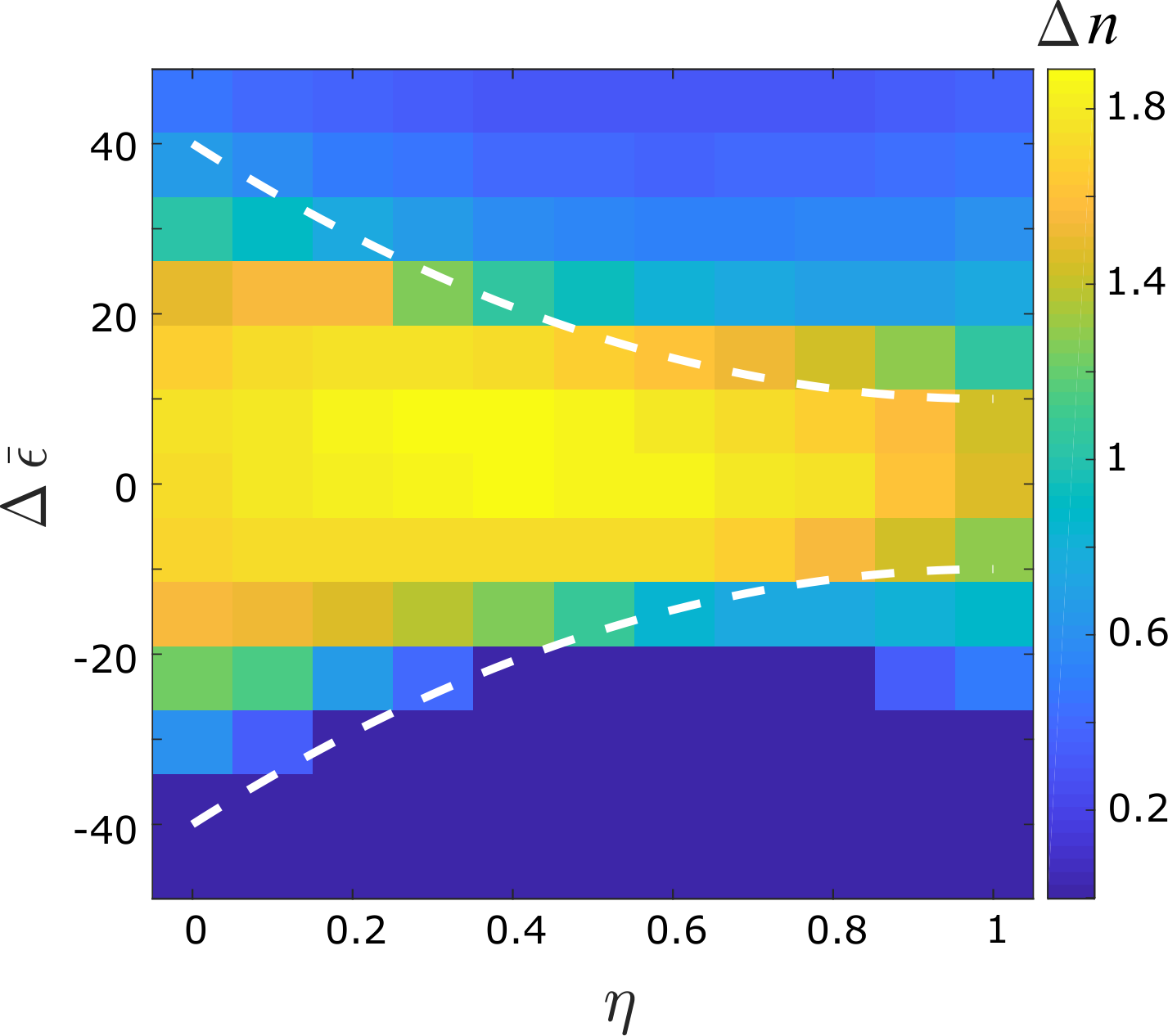
In Fig. 9 we plot the width of the OSM phase averaged over the angles and , which is obtained from the numerical minimization of Eq. (19). Here and mark the boundaries of the OSM phase per angle (maximal value is 2), as shown in Fig. 4 .(c). The white dashed line is the analytic estimate Eq. (25). We thus, conclude that the OSM phase is not sensitive to parameters and is a generic feature of the phase diagram of electron doped moiré TMDs.
Appendix E Spin Exchange interactions and expected phenomenology
Inside the OSM phase charge fluctuations of the localized species are quenched and therefore, the relevant inter-species interactions are of spin-exchnage type. In this section we discuss two such interactions and their possible influence on the magnetic ground state.
We anticipate that the ferromagnetic Hund’s coupling is the largest exchnage mechanism
| (26) |
where is the spin of the localized moments at site (let us assume they belong to species ) . Using standard harmonic oscillator states, we estimate .
Upon approaching the meting point of the OSM state however, other interaction terms that compete with Eq. (26). For example, the interaction that scatters across the original Brillouin zone. To see this let us first write this term in basis of the original operators Eq. (1) , where (for an angle of we obtain ). Taking into account the moiré potential and the slave-rotor decomposition described above, this interaction assumes the form
| (27) |
where . Thus, when the band is localized and this term vanishes. However, if the local moments are incorporated into the Fermi surface (through the formation of a heavy Fermi liquid) they reacquire a finite quasi-particle weight Chen et al. 2020b. Thus, this interaction can become important close to the melting point of the local moment lattice.
As mentioned above, inside the OSM phase we expect the dominant exhnage to be Hind’s and therefore spin-correlations to be ferromagnetic as in Ref. Anisimov et al. 2002. When the Hund’s coupling Eq. (26) is dominant the main influence of the itinerant electrons inside the OSM state is to mediate long-ranged RKKY interactions Fischer and Klein 1975
| (28) |
where is the density of states. Thus, as the filling of the itinerant band is modified from zero to 2, the nearest-neighbour interaction mediated by the electrons can be tuned from ferromagnetic in the dilute limit to antiferromagnetic and back to ferromagnetic (going through a van Hove singularity). This interaction is added to the direct superxchnage between sites Wu et al. 2018, which may have a cooperative effect or frustrate the magnetic interactions.
Appendix F The heavy Fermi liquid state
When the antiferromagnetic correlations dominate we expect a heavy-Fermi liquid state to compete with the internal magnetic interactions. For completeness, in this appendix we compute the Kondo temperature assuming meV within the large-N mean-field theory Hewson 1997. We find hat 5-15 K inside the OSM phase and therefore, we expect that if the antiferromagnetic correlations dominate the OSM melting transition can be accompanied by a detectable heavy Fermi liquid state. Moreover, in this case the tunability of the itinerant electron density may allow to tune though the Doniach phase diagram Doniach 1977.

Let us breifly describe the large-N mean field theory. The dispersion of the two species is taken to be
| (29) |
where the density of each species is set separately using the Lagrange multipliers according to their values in the slave-rotor mean-field calculation. We then decouple Eq. (27) using the mean-field hybridization . We then solve for self-consistently, while tuning and to conserve the density of and on average. The Kondo temperature is then estimated by seeking the lowest temperature where the self-consistent solution for . To obtain the Kondo temperature we estimate the lowest temperature where .
In Fig. 10 we plot the resulting Kondo temperature as a function of twist-angle and density for meV. As can be seen, the Kondo temperature measurable in standard cryosthetics and might be physically important.
References
- Bistritzer and MacDonald (2011) R. Bistritzer and A. H. MacDonald, Proceedings of the National Academy of Sciences 108, 12233 (2011).
- Cao et al. (2018a) Y. Cao, V. Fatemi, S. Fang, K. Watanabe, T. Taniguchi, E. Kaxiras, and P. Jarillo-Herrero, Nature 556, 43 (2018a).
- Yankowitz et al. (2019) M. Yankowitz, S. Chen, H. Polshyn, Y. Zhang, K. Watanabe, T. Taniguchi, D. Graf, A. F. Young, and C. R. Dean, Science 363, 1059 (2019).
- Lu et al. (2019) X. Lu, P. Stepanov, W. Yang, M. Xie, M. A. Aamir, I. Das, C. Urgell, K. Watanabe, T. Taniguchi, G. Zhang, et al., Nature 574, 653 (2019).
- Balents et al. (2020) L. Balents, C. R. Dean, D. K. Efetov, and A. F. Young, Nature Physics 16, 725 (2020).
- Cao et al. (2018b) Y. Cao, V. Fatemi, A. Demir, S. Fang, S. L. Tomarken, J. Y. Luo, J. D. Sanchez-Yamagishi, K. Watanabe, T. Taniguchi, E. Kaxiras, et al., Nature 556, 80 (2018b).
- Chen et al. (2019) G. Chen, L. Jiang, S. Wu, B. Lyu, H. Li, B. L. Chittari, K. Watanabe, T. Taniguchi, Z. Shi, J. Jung, et al., Nature Physics 15, 237 (2019).
- Jiang et al. (2019) Y. Jiang, X. Lai, K. Watanabe, T. Taniguchi, K. Haule, J. Mao, and E. Y. Andrei, Nature 573, 91 (2019).
- Kerelsky et al. (2019) A. Kerelsky, L. J. McGilly, D. M. Kennes, L. Xian, M. Yankowitz, S. Chen, K. Watanabe, T. Taniguchi, J. Hone, C. Dean, et al., Nature 572, 95 (2019).
- Cao et al. (2020) Y. Cao, D. Rodan-Legrain, J. M. Park, F. N. Yuan, K. Watanabe, T. Taniguchi, R. M. Fernandes, L. Fu, and P. Jarillo-Herrero, arXiv preprint arXiv:2004.04148 (2020).
- Zondiner et al. (2020) U. Zondiner, A. Rozen, D. Rodan-Legrain, Y. Cao, R. Queiroz, T. Taniguchi, K. Watanabe, Y. Oreg, F. von Oppen, A. Stern, et al., Nature 582, 203 (2020).
- Wong et al. (2020) D. Wong, K. P. Nuckolls, M. Oh, B. Lian, Y. Xie, S. Jeon, K. Watanabe, T. Taniguchi, B. A. Bernevig, and A. Yazdani, Nature 582, 198 (2020).
- Chen et al. (2020a) G. Chen, A. L. Sharpe, E. J. Fox, Y.-H. Zhang, S. Wang, L. Jiang, B. Lyu, H. Li, K. Watanabe, T. Taniguchi, et al., Nature 579, 56 (2020a).
- Serlin et al. (2020) M. Serlin, C. Tschirhart, H. Polshyn, Y. Zhang, J. Zhu, K. Watanabe, T. Taniguchi, L. Balents, and A. Young, Science 367, 900 (2020).
- Po et al. (2018) H. C. Po, L. Zou, A. Vishwanath, and T. Senthil, Physical Review X 8, 031089 (2018).
- Song et al. (2019) Z. Song, Z. Wang, W. Shi, G. Li, C. Fang, and B. A. Bernevig, Physical review letters 123, 036401 (2019).
- Kang and Vafek (2018) J. Kang and O. Vafek, Physical Review X 8, 031088 (2018).
- Yuan and Fu (2018) N. F. Q. Yuan and L. Fu, Physical Review B 98, 045103 (2018).
- Wu et al. (2018) F. Wu, T. Lovorn, E. Tutuc, and A. H. MacDonald, Phys. Rev. Lett. 121, 026402 (2018).
- Zhang et al. (2019) Y. Zhang, N. F. Yuan, and L. Fu, arXiv preprint arXiv:1910.14061 (2019).
- Wang et al. (2020) L. Wang, E.-M. Shih, A. Ghiotto, L. Xian, D. A. Rhodes, C. Tan, M. Claassen, D. M. Kennes, Y. Bai, B. Kim, et al., Nature materials , 1 (2020).
- Regan et al. (2020) E. C. Regan, D. Wang, C. Jin, M. I. B. Utama, B. Gao, X. Wei, S. Zhao, W. Zhao, Z. Zhang, K. Yumigeta, et al., Nature 579, 359 (2020).
- Xu et al. (2020a) Y. Xu, S. Liu, D. A. Rhodes, K. Watanabe, T. Taniguchi, J. Hone, V. Elser, K. F. Mak, and J. Shan, Nature 587, 214 (2020a).
- Xu et al. (2020b) Y. Xu, S. Liu, D. A. Rhodes, K. Watanabe, T. Taniguchi, J. Hone, V. Elser, K. F. Mak, and J. Shan, arXiv preprint arXiv:2007.11128 (2020b).
- Li et al. (2021a) T. Li, S. Jiang, L. Li, Y. Zhang, K. Kang, J. Zhu, K. Watanabe, T. Taniguchi, D. Chowdhury, L. Fu, J. Shan, and K. F. Mak, “Continuous mott transition in semiconductor moiré superlattices,” (2021a), arXiv:2103.09779 [cond-mat.str-el] .
- Doniach (1977) S. Doniach, physica B+ C 91, 231 (1977).
- Steglich et al. (1979) F. Steglich, J. Aarts, C. D. Bredl, W. Lieke, D. Meschede, W. Franz, and H. Schäfer, Physical Review Letters 43, 1892 (1979).
- Stewart (1984) S. G. Stewart, Reviews of Modern Physics 56, 755 (1984).
- Nakatsuji and Maeno (2000) S. Nakatsuji and Y. Maeno, Physical review letters 84, 2666 (2000).
- Anisimov et al. (2002) V. Anisimov, I. Nekrasov, D. Kondakov, T. Rice, and M. Sigrist, The European Physical Journal B-Condensed Matter and Complex Systems 25, 191 (2002).
- Löhneysen et al. (1998) H. Löhneysen, S. Mock, A. Neubert, T. Pietrus, A. Rosch, A. Schröder, O. Stockert, and U. Tutsch, Journal of magnetism and magnetic materials 177, 12 (1998).
- von Löhneysen (1996) H. von Löhneysen, Journal of Physics: Condensed Matter 8, 9689 (1996).
- Von Loehneysen et al. (1998) H. Von Loehneysen, A. Neubert, T. Pietrus, A. Schröder, O. Stockert, U. Tutsch, M. Loewenhaupt, A. Rosch, and P. Wölfle, The European Physical Journal B-Condensed Matter and Complex Systems 5, 447 (1998).
- Schröder et al. (2000) A. Schröder, G. Aeppli, R. Coldea, M. Adams, O. Stockert, H. Löhneysen, E. Bucher, R. Ramazashvili, and P. Coleman, Nature 407, 351 (2000).
- Senthil et al. (2003) T. Senthil, S. Sachdev, and M. Vojta, Physical review letters 90, 216403 (2003).
- Stewart (2001) G. R. Stewart, Rev. Mod. Phys. 73, 797 (2001).
- Custers et al. (2003) J. Custers, P. Gegenwart, H. Wilhelm, K. Neumaier, Y. Tokiwa, O. Trovarelli, C. Geibel, F. Steglich, C. Pépin, and P. Coleman, Nature 424, 524 (2003).
- Senthil et al. (2004) T. Senthil, M. Vojta, and S. Sachdev, Phys. Rev. B 69, 035111 (2004).
- Coleman (2007) P. Coleman, Handbook of magnetism and advanced magnetic materials (2007).
- Gegenwart et al. (2008) P. Gegenwart, Q. Si, and F. Steglich, nature physics 4, 186 (2008).
- Vojta (2010) M. Vojta, Journal of Low Temperature Physics 161, 203 (2010).
- Yuan et al. (2003) H. Yuan, F. Grosche, M. Deppe, C. Geibel, G. Sparn, and F. Steglich, Science 302, 2104 (2003).
- Aoki et al. (2019) D. Aoki, K. Ishida, and J. Flouquet, Journal of the Physical Society of Japan 88, 022001 (2019).
- Jiao et al. (2020) L. Jiao, S. Howard, S. Ran, Z. Wang, J. O. Rodriguez, M. Sigrist, Z. Wang, N. P. Butch, and V. Madhavan, Nature 579, 523 (2020).
- Liu et al. (2013) G.-B. Liu, W.-Y. Shan, Y. Yao, W. Yao, and D. Xiao, Phys. Rev. B 88, 085433 (2013).
- Biermann et al. (2005) S. Biermann, L. de’Medici, and A. Georges, Physical review letters 95, 206401 (2005).
- Florens and Georges (2004) S. Florens and A. Georges, Phys. Rev. B 70, 035114 (2004).
- Zhao and Paramekanti (2007) E. Zhao and A. Paramekanti, Phys. Rev. B 76, 195101 (2007).
- Chen et al. (2020b) C. Chen, I. Sodemann, and P. A. Lee, “Competition of spinon fermi surface and heavy fermi liquids states from the periodic anderson to the hubbard model,” (2020b), arXiv:2010.00616 [cond-mat.str-el] .
- (50) This shift can be absorbed into .
- Laturia et al. (2018) A. Laturia, M. L. Van de Put, and W. G. Vandenberghe, npj 2D Materials and Applications 2, 1 (2018).
- (52) We neglect the angle dependence of .
- (53) One should note the regions where the densities of the different species are locked to the value . These regions correspond to a band insulator in the relevant species, where the corresponding band is completely filled with two particles per moiré unit cell.
- Keselman et al. (2020a) A. Keselman, L. Savary, and L. Balents, SciPost Physics (2020a).
- Keselman et al. (2020b) A. Keselman, B. Bauer, C. Xu, and C.-M. Jian, Physical Review Letters 125, 117202 (2020b).
- Wu et al. (2019) F. Wu, T. Lovorn, E. Tutuc, I. Martin, and A. H. MacDonald, Physical review letters 122, 086402 (2019).
- Zhang et al. (2021) Y.-H. Zhang, D. N. Sheng, and A. Vishwanath, “An chiral spin liquid and quantized dipole hall effect in moiré bilayers,” (2021), arXiv:2103.09825 [cond-mat.str-el] .
- Fischer and Klein (1975) B. Fischer and M. W. Klein, Physical Review B 11, 2025 (1975).
- (59) We note that this transition line will be pushed to larger upon increase of the interaction parameter .
- Rozen et al. (2020) A. Rozen, J. M. Park, U. Zondiner, Y. Cao, D. Rodan-Legrain, T. Taniguchi, K. Watanabe, Y. Oreg, A. Stern, E. Berg, P. Jarillo-Herrero, and S. Ilani, “Entropic evidence for a pomeranchuk effect in magic angle graphene,” (2020), arXiv:2009.01836 [cond-mat.mes-hall] .
- Saito et al. (2020) Y. Saito, F. Yang, J. Ge, X. Liu, K. Watanabe, T. Taniguchi, J. I. A. Li, E. Berg, and A. F. Young, “Isospin pomeranchuk effect and the entropy of collective excitations in twisted bilayer graphene,” (2020), arXiv:2008.10830 [cond-mat.mes-hall] .
- Joshua et al. (2012) A. Joshua, S. Pecker, J. Ruhman, E. Altman, and S. Ilani, Nature communications 3, 1 (2012).
- Ramires and Lado (2021) A. Ramires and J. L. Lado, “Emulating heavy fermions in twisted trilayer graphene,” (2021), arXiv:2102.03312 [cond-mat.mes-hall] .
- Li et al. (2021b) H. Li, S. Li, M. H. Naik, J. Xie, X. Li, E. Regan, D. Wang, W. Zhao, K. Yumigeta, M. Blei, T. Taniguchi, K. Watanabe, S. Tongay, A. Zettl, S. G. Louie, M. F. Crommie, and F. Wang, “Imaging local discharge cascades for correlated electrons in ws2/wse2 moiré superlattices,” (2021b), arXiv:2102.09986 [cond-mat.mes-hall] .
- Hewson (1997) A. C. Hewson, The Kondo problem to heavy fermions, 2 (Cambridge university press, 1997).