Analytic Light Curves in Reflected Light:
Phase Curves, Occultations, and Non-Lambertian Scattering for
Spherical Planets and Moons
astroquery (Ginsburg et al. 2013; Ginsburg et al. 2019),
Eigen v3 (Guennebaud et al. 2010),
exoplanet (Foreman-Mackey et al. 2020),
pybind11 (Jakob et al. 2017),
pymc3 (Salvatier et al. 2016),
scipy (Jones et al. 2001),
starry (Luger et al. 2018),
theano (Theano Development Team 2016).
Abstract
We derive efficient, closed form, differentiable, and numerically stable solutions for the flux measured from a spherical planet or moon seen in reflected light, either in or out of occultation. Our expressions apply to the computation of scattered light phase curves of exoplanets, secondary eclipse light curves in the optical, or future measurements of planet-moon and planet-planet occultations, as well as to photometry of solar system bodies. We derive our solutions for Lambertian bodies illuminated by a point source, but extend them to model illumination sources of finite angular size and rough surfaces with phase-dependent scattering. Our algorithm is implemented in Python within the open-source starry mapping framework and is designed with efficient gradient-based inference in mind. The algorithm is orders of magnitude faster than direct numerical evaluation methods and orders of magnitude more precise. We show how the techniques developed here may one day lead to the construction of two-dimensional maps of terrestrial planet surfaces, potentially enabling the detection of continents and oceans on exoplanets in the habitable zone.
Keywords:
methods: analytic — techniques: photometricI Introduction
Despite recent advances in instrumentation and the dawn of thirty meter-class telescopes and kilometer-wide interferomer arrays, extrasolar planets will remain unresolved point sources for decades to come. Nevertheless, modulations in the light received from these distant bodies due to their rotation, changing illumination, and eclipses by their host stars or other bodies in the system can be harnessed to reconstruct two-dimensional views of their surfaces. In particular, next-generation space-based telescopes such as the Large UV/Optical/IR Surveyor (LUVOIR) may enable us to measure variations in the reflected light signature of terrestrial planets in the habitable zone, which can be used to map their surfaces and indirectly infer the presence of clouds, continents, oceans, and perhaps even life.
There is an extensive literature on techniques for mapping exoplanet surfaces based on their phase curves (Russell 1906; Lacis & Fix 1972; Knutson et al. 2007; Cowan & Agol 2008; Oakley & Cash 2009; Berdyugina & Kuhn 2017; Luger et al. 2021b; Luger et al. 2021a; Heng et al. 2021, e.g.,) and occultation light curves (Williams et al. 2006; Rauscher et al. 2007; Majeau et al. 2012; de Wit et al. 2012; Rauscher et al. 2018, e.g.,), both in thermal and reflected (scattered) light. In particular, much attention has been given to techniques for mapping Earth-like planets from visible-light reflected phase curves (Ford et al. 2001; Kawahara & Fujii 2010; Kawahara & Fujii 2011; Fujii & Kawahara 2012; Kawahara 2020; Aizawa et al. 2020, e.g.,). Unlike thermal phase curves, which primarily encode (often degenerate) information about longitudinal surface brightness variations (Russell 1906), reflected light curves often contain information about the full two-dimensional surface albedo distribution (Kawahara & Fujii 2010, e.g.,).
Occultation light curves in reflected light can encode even more information about the surface. Thus far, these have been studied primarily within our solar system. Mutual occultations among the Galilean moons of Jupiter have been extensively studied to infer surface properties of the moons and to refine their ephemerides (Arlot et al. 1974; Aksnes et al. 1984; Arlot et al. 2014; de Kleer et al. 2017; Saquet et al. 2018; Morgado et al. 2019; Bartolić et al. 2021, e.g.,). Farther out in the solar system, mutual occultations of Pluto and Charon in the late 1980s were used to confirm Charon’s existence (Stern 1992), establish the sizes and orbital parameters of the two bodies (Tholen & Buie 1990), and infer their surface properties (Marcialis 1990). In particular, Dunbar & Tedesco 1986 developed an efficient analytic algorithm to model Pluto-Charon occultation light curves in reflected light assuming uniform surfaces and used it to infer the two body’s average geometrical albedos. Later, Buie et al. 1992 used a maximum entropy approach to reconstruct two-dimensional maps of the two bodies and Reinsch et al. 1994 analyzed the complete mutual occultation dataset to infer longitudinal maps of Pluto’s albedo.
Many studies have analyzed real Earth reflected light curves to infer surface properties of our planet as an exercise in prepartion for the mapping of exoplanets. Cowan et al. 2009 and Cowan et al. 2011 analyzed visible-light disk-integrated light curves of the Earth taken by the Deep Impact spacecraft to produce longitudinal maps of the surface, harnessing multi-band observations to disentangle static surface brightness features from temporally variable clouds. A transit of Earth by the Moon was observed as well (Livengood et al. 2011), although this data has yet to be exploited for mapping purposes. More recently, Jiang et al. 2018 and Fan et al. 2019 used data from the L1-stationed DSCOVR satellite to infer surface and cloud properties of the Earth, and Luger et al. 2019b analyzed background scattered light in TESS photometry to reconstruct a cloud map of the Earth.
On the open-source software front, Louden & Kreidberg 2018 developed spiderman, an efficient discretization scheme on the sphere that enables fast computation of exoplanet phase curves and occultation light curves in Python. Haggard & Cowan 2018 presented EARL (Exoplanet Analytic Reflected Lightcurves), a Mathematica code to compute analytic, closed form solutions for the phase curve of a Lambert sphere, i.e., one that scatters light isotropically, in the case that the surface albedo distribution is characterized by either a sum of delta functions or a sum of spherical harmonics. Farr et al. 2018 released exocartographer, a Bayesian framework for doing inference on exoplanet phase curves based on a HEALPix (Górski et al. 2005) discretization scheme. Finally, Luger et al. 2019a introduced starry, a light curve modeling package that computes thermal phase curves and occultation light curves, as well as their derivatives, analytically from a spherical harmonic expansion of the surface brightness.
The present paper is an extension to the starry algorithm, adapting it to model phase curves and occultation light curves in reflected light. The expressions we derive are analytic: they may all be expressed in closed form in terms of algebraic operations involving trigonometric functions and (at times) elliptic integrals. We derive numerically stable recursion relations for the efficient evaluation of all expressions and code them within an autodifferentiation framework to enable the computation of accurate derivatives for use in gradient-based inference and optimization schemes. Our code is fully open-source, comprehensively unit-tested, and supplemented with an extensive API documentation and suite of tutorials. As in all papers in the starry series, in the caption of each of the figures we provide links to the exact Python scripts that generated them. Next to many of the equations we also provide links to Jupyter notebooks containing detailed derivations and/or validations.
II Overview
Our goal in this paper is to derive analytic expressions for the flux received by a distant observer from a sphere of non-uniform albedo illuminated by a monochromatic source that may or may not be occulted by a (possibly different) spherical body. This applies, for example, to the case of planetary phase curves, secondary eclipse (occultation) light curves, and moon-moon, planet-moon, and planet-planet occultations (in the Solar System or not), all seen in reflected light. We derive all expressions in the limit that the reflecting body is Lambertian, i.e., it scatters light isotropically, but we relax this assumption in later sections. We model the general case of an intensity that varies across the surface of the body according to a spatially-dependent albedo . Throughout this paper, we will take to mean the spherical albedo, the fraction of power incident on a body at a given wavelength that is scattered back out to space (in all directions). Note that the spherical albedo is closely related to the Bond albedo: the Bond albedo is the stellar flux-weighted integral of over all wavelengths (Seager 2010, see, e.g.,).
As in Luger et al. 2019a, we compute fluxes by first expanding the surface in terms of spherical harmonics. While in Luger et al. 2019a we expanded the emissivity of the surface, here we instead expand the spherical albedo . Specifically, if is the vector of spherical harmonic coefficients describing the albedo anywhere on the surface and is the spherical harmonics basis (Equation A1), the albedo at a point on the sky-projected disk of the body is given by the dot product
| (1) |
The flux measured from this body is proportional to the surface integral over the projected disk of the albedo times the illumination profile of the surface, given by Lambert’s law as
| (2) |
where is the angle between the incident radiation and the surface normal and is the peak illumination. We show in Appendix A.2 that in the case of, say, a planet illuminated by its host star,
| (3) |
where is the distance between the planet and the star (in units of the planet’s radius) and is the stellar flux measured at the observer (in arbitrary units). Following the convention in Luger et al. 2019a, we assume throughout this paper that , so all fluxes are defined as a fraction of the flux of the illumination source at the observer.
The piecewise nature of the illumination function at the day/night terminator makes the problem of computing the visible flux particularly difficult; most studies to date have tackled the problem numerically, either via Monte Carlo integration (Ford et al. 2001, e.g.,) or by discretizing the surface and computing the relevant integrals by summing over the visible pixels (Kawahara & Fujii 2010; Fujii & Kawahara 2012, e.g.,). Recently, Haggard & Cowan 2018 developed an analytic framework for computing light curves of unocculted bodies illuminated by a point source. In this paper, we re-derive their solution under the starry framework and extend it for the first time to the case where the body is occulted by another spherical body, which may or may not be the illumination source. We also extend the solution to the case of an extended illumination source and to non-Lambertian scattering.
In Luger et al. 2019a, we reduced the problem of computing the flux from an occulted body in thermal (emitted) light to a series of efficient, analytical operations involving trigonometric functions of the position and size of the occultor and certain complete elliptic integrals. In the case of reflected light, however, the change in the limits of integration due to the unilluminated night side breaks many of the symmetries that simplified the flux calculation. In particular, the limits of integration now depend on the solution to a quartic equation specifying the points of intersection between the occultor and the day/night terminator, and the solution to those integrals is now a function of incomplete elliptic integrals. The procedure for computing the flux is therefore significantly more complex. We therefore defer all calculations to the Appendix, and devote the body of the paper to validating and demonstrating applications of our approach.
This paper is organized as follows. In §III we present sample light curves computed using our algorithm, validate it against numerical integration, and discuss its performance in terms of computational speed and precision. In §IV we extend the model to apply to illumination sources of finite size and surfaces that scatter light anisotropically. We discuss implications, applications, and limitations of our model in §V and summarize our findings in §VI. For convenience, Tables 1–4 at the end list all symbols and variables used in the text, with descriptions and links to the equations in which they are defined.

III Reflected light curves in starry
III.1 Sample light curves
Figure 1 shows a sample application of the algorithm developed in this paper: a reflected light phase curve of the Earth over the course of one year. The model is computed using the methodology in Appendix B from an spherical harmonic expansion of the cloudless Earth, where the oceans are given an albedo of zero and the continents an albedo of unity (note, however, that since the light curve is normalized, the model does not depend on the value of the latter). The Earth is assumed to be a perfect Lambertian scatterer, so effects like the phase dependence of Rayleigh scattering and specular reflection (glint) from the oceans are neglected (but see §IV for an extension of the model to non-Lambertian scatterers). The observer is assumed to be along the ecliptic, so the illumination source is along the plane of a right-handed Cartesian coordinate system, with pointing toward the observer and pointing to the right on the sky. The axis of rotation of the Earth is therefore tilted clockwise away from by . The images at the top show snapshots of the disk of the Earth throughout the observation; below each one, we plot in blue the normalized phase curve at that phase over a single rotation. The orange dots correspond to a brute force numerical solution, obtained by discretizing the disk on a grid of points and summing over the dayside. The models agree to within the numerical precision of the brute force solution (about 100 ppm of the planetary flux in this case).
While the dominant signal in the phase curve is the sine-like envelope due to the changing phases of the Earth, the local behavior of the light curve at each phase is complex and varies significantly over the course of the year. Unlike phase curves in thermal light, which primarily encode low-order spatial information (since the region of integration is always the full disk), phase curves in reflected light encode information at different scales depending on the phase. At crescent phase, the region of the disk contributing to the total flux is a narrow lune; these measurements therefore encode information primarily about high- modes. At full phase, the region of integration is the full disk, so these measurements encode information about low- modes. Furthermore, because of the obliquity of the Earth, the orientation of the crescent lune changes relative to features on the surface over the course of one orbit, changing the relative contribution of different portions of the surface to the flux and increasing the overall information content of the observation. As we will show in §V.2, the information content of reflected light phase curves is overwhelmingly higher than that of phase curves in thermal light, particularly for planets with significant obliquity.


Figure 2 shows another light curve of the rotating Earth, but this time taken during an occultation by the Moon. The map of the Earth is the same as before, but the observer is now along the equatorial plane of the Earth. The top panel is a reproduction of Figure 7 in Luger et al. 2019a for the case of thermal light, where the Moon is seen to travel across the disk of the Earth from southwest to northeast, progressively occulting South America (dip), the Atlantic (peak), and Africa (dip). As before, the blue curve is the analytic solution and the orange dots correspond to the numerical solution.
The bottom panel of the figure shows a light curve for the same occultation geometry, but seen instead in reflected light, with the Sun to the top left and slightly out of the page, corresponding to some point during northern summer. Note the same dip-peak-dip pattern, albeit with significantly different amplitudes. In particular, the transit across South America is deeper, since it occurs close to local noon, when the illumination is highest; conversely, the transit across Africa occurs close to local dusk, when the illumination is close to zero. As before, the light curves computed using starry agree to within the numerical precision of the brute force solution.


Our last sample light curve is Figure 3, which shows a secondary eclipse light curve of the Earth as it is occulted by the Sun. The model for the Earth is the same as above, and the observer is now close to the ecliptic, but slightly misaligned so that the Earth is occulted behind a solar latitude of (i.e., at a solar impact parameter of ). The observation takes place at the June solstice, so the Earth is tilted by out of the page. As before, the top panel shows the light curve in thermal light; this is similar to the top panel of Figure 13 in Luger et al. 2019a. The orange dots again correspond to the numerical solution. The center panel shows the same light curve in reflected light. Because the observation occurs very close to full phase, the normalized light curves look very similar to each other. The bottom panel shows the difference between the two (reflected minus thermal), which is only on the order of a few percent. In fact, because the illumination profile is proportional to the cosine of the viewing angle, , and the reflection is assumed to be isotropic, the (normalized) secondary eclipse light curve in reflected light is to good approximation equal to a limb-darkened thermal occultation light curve with linear limb darkening coefficient . As we will see later, for very close-in planets this approximation breaks down, since the illumination phases at secondary eclipse ingress and egress are sufficiently different from full phase.
III.2 Performance
As we discuss in the Appendix, the model for phase curves and occultation light curves in reflected light may be expressed analytically in terms of purely algebraic and trigonometric functions and in some cases incomplete elliptic integrals of the first, second, and third kinds. We have derived efficient and numerically stable recursion relations to compute the relevant expressions and their derivatives. At times, these involve the evaluation of certain expressions numerically, especially when doing so leads to either a speed-up or a significant gain in numerical precision. In particular, as we discuss in Appendix C.1, the integration boundaries during an occultation sometimes depend on the solution to a quartic equation. While this can be solved in closed form, the analytic solution can often be very unstable. We therefore solve the quartic numerically, attaining a precision for the roots within a few orders of magnitude of machine (double) precision.
Figures 4 and 5 summarize the precision and computation time of the starry algorithm for two typical scenarios: a phase curve evaluation (Figure 4) and an occultation evaluation (Figure 5). Blue points correspond to the reflected light algorithm developed in this paper, while purple points correspond to the thermal light algorithm from Luger et al. 2019a for the same occultation geometry, but without an illumination source. Solid and dashed lines correspond to evaluations without and with gradient propagation, respectively (see §III.3 for details). The orange and red dots correspond to numerical evaluation of the flux: brute force integration by summation on a grid of points (orange) and two-dimensional adaptive Gaussian quadrature using the dblquad function in scipy (Jones et al. 2001) with both absolute and relative error tolerances set to (red). In both figures, the vertical axis corresponds to the evaluation time in seconds for a single flux computation, while the size of the points is proportional to the base-10 log of the relative error. For the starry solutions, the latter is estimated as the max-min difference in the flux over one thousand evaluations in which the input parameters are perturbed within an order of magnitude of machine epsilon; this is therefore a probe of the condition number of the starry algorithm and captures only error due to numerical instabilities. It is worth emphasizing that this is a measurement of the precision of the algorithm, rather than the accuracy, because it would be computationally intractable to compute a solution more accurate than this using a different algorithm. We argue that this measurement can be interpreted to mean that the algorithm is also accurate, but detailed quantification of this difference is beyond the scope of this paper. For the numerical solutions, the error is estimated as the difference between the numerical flux and the starry flux.
For both phase curves and occultations, the starry reflected light algorithm is 1–2 orders of magnitude slower than the emitted light algorithm, owing primarily to the increased complexity of the reflected light model. For phase curves (Figure 4), the thermal solution vector (Equation A7) is a constant that can be pre-computed, while the analogous vector in the reflected light case, (Equation B2), must be evaluated recursively each time. For occultations (Figure 5), the slower evaluation in the reflected light case is primarily due to the time spent solving the quartic equation for the points of intersection between the occultor and the day/night terminator of the illuminated body (Appendix C). This contributes the same overhead at all map degrees , resulting in a gentler scaling in than for the thermal case; for large , the evaluation time for the two algorithms is within a factor of 2–3. In terms of precision, the algorithms are comparable, particularly for occultations. For both phase curves and occultations, the numerical error up to is less than one part per trillion () for both thermal and reflected light curves.
Compared to either numerical evaluation method, the starry reflected light solutions are 4–5 orders of magnitude faster and about 10 orders of magnitude more precise. While different grid sizes and different error settings for the numerical integration change the balance slightly between these numbers, the starry solution is always many orders of magnitude faster and more precise than either method. In particular, because of the complicated integration boundaries (see, for example, Figure 15), two-dimensional Gaussian quadrature struggles to reach adequate accuracy in a reasonable amount of time, while integration on a grid fails to capture the curvature of the integration boundaries. Moreover, neither method yields the gradient of the solution with respect to the input parameters, which can be extremely useful for optimization and inference problems (see §III.3) below.
Note, importantly, that as we mentioned above, the reported error of the starry solution is only the numerical error of the algorithm: it does not capture any systematic error due to, say, an error in the derivation of the method. To this end, we rely on the Jupyter notebooks containing derivations and validations of the main equations in the Appendix, whose links appear next to the equation labels. We have also developed an extensive suite of unit tests comparing the starry solution to the numerical solution over a large grid of input parameter values, and verified that the solutions agree to within the precision of the numerical method. That said, there are specific cases in which the algorithm presented in the Appendix suffers from numerical instabilities. These generally happen due to division by small numbers or catastrophic cancellation in the recursion, and often occur near configurations involving grazing occultations, near-total occultations, terminator semi-minor axis or , etc. To mitigate these, we introduce various tolerance parameters in the code to either nudge the inputs away from these singular points or switch to a different evaluation method. These parameters are outlined in Table 5 at the end. In the vicinity of the cases described in that table, the precision of the starry algorithm will be reduced to (roughly) the value of the tolerance parameter, which in extremely rare cases can be as high as .
III.3 Implementation and usage
The algorithm presented in this paper has been implemented in the Python package starry, which can be installed from GitHub or via the Python package manager pip. The algorithm is coded in a mixture of C++ with forward automatic differentiation using the Eigen library (Guennebaud et al. 2010) and Python with backward differentiation using just-in-time compiled theano operations (Theano Development Team 2016). The user interface, however, is purely in Python. The theano backend facilitates integration with the exoplanet modeling package (Foreman-Mackey et al. 2020) and in particular with pymc3 (Salvatier et al. 2016) for inference with gradient-based Markov Chain Monte Carlo (MCMC) schemes such as Hamiltonian Monte Carlo (Duane et al. 1987, HMC;) and No-U-Turn Sampling (Hoffman & Gelman 2011, NUTS;). Complete documentation and an extensive library of tutorials is available online. The links next to each of the figures point to the Python scripts used to generate them and may also help in learning how to use starry.
IV Extensions
The algorithm discussed above and derived in the Appendix computes light curves in the limit that (1) the body is illuminated by a point source and (2) the body is an ideal Lambertian scatterer. Both of these assumptions can be relaxed within starry, and below we discuss modifications to the code to allow for this.
IV.1 Extended illumination source
In the limit that the angular size of the star as seen from the planet is small, the illumination profile on the surface of the planet will decrease as the cosine of the angle between the surface normal and the star, reaching zero at the day/night terminator, an angle away from the sub-stellar point. However, if the star is sufficiently large and the planet is sufficiently close-in, rays originating from near the limb of the star will reach points on the planet surface beyond this angle. If the stellar radius is larger than the planet radius , the angular extent of the true day/night terminator past is given by
| (4) |
where the semi-major axis of the orbit (where we implictly assume the eccentricity is zero). For planets like the Earth, this quantity is only about , resulting in a negligible effect on the planet’s light curve. However, for very close-in planets, the effect can be significant. For instance, the hot Jupiter Kelt-9b has and planet (Wong et al. 2019). Assuming zero eccentricity and ignoring any stellar oblateness (Ahlers et al. 2020, see), the day/night terminator extends past the limb of that planet. Figure 6 shows the illumination profile of this planet in a Mollweide projection, with the sub-stellar point at the center, for the point source approximation (left) and accounting for the finite size of the star (right). In addition to the displaced day/night terminator, the main difference between the two profiles is the sub-stellar intensity, which is significantly higher in the extended source case. This is due to the simple fact that in the point source case the illumination source is placed at the center of the star, which is one stellar radius farther from the planet than the point closest to the planet (the sub-planetary point) in the extended source case. Once accounting for this difference, the fractional change in the intensity on the planet away from the sub-stellar point is similar in both cases, and the intensity anywhere beyond is less than one-tenth the peak value.

The illumination profile in the extended source case may be computed as the two-dimensional integral of the point source illumination profile over the visible portion of the stellar disk. While this integral may in theory be computed analytically (see, for instance, Kopal 1954, who derived series solutions to this problem), the resulting profile on the planet surface will not in general be exactly expressible in terms of spherical harmonics, a necessary condition for the starry algorithm. For simplicity, we therefore compute the illumination profile for extended sources by averaging the contribution of source_npts point sources uniformly distributed across the projected disk corresponding to the portion of the stellar surface visible from the planet, where source_npts is a user-supplied value. In the limit , this is a spherical cap centered at the sub-planet point with radius . In Figure 6 we set source_npts = 300, but in practice we find that points are sufficient for even the most extreme cases such as Kelt-9b. Note, importantly, that while this method allows one to account for the effect of stellar limb darkening on the illumination profile of the planet, this has not been implemented in starry.
Figure 7 shows the practical implications of the finite stellar size for the phase curve of Kelt-9b. The left panel shows the reflected light phase curve of the planet in parts per million, assuming a spherical albedo of 0.2, for the point source approximation (blue) and including the effect of the extended source with source_npts = 300 (purple). The increased illumination at the sub-stellar point results in a ppm increase in the value of the phase curve close to full phase (). Close to a phase of zero, the extended source results in decreased flux, since the portion of the star illuminating the planet (the region close to the limb) is slightly farther away, by a factor of . This results in a steeper phase curve, which can be seen in the right panel, where the light curves have been normalized to their maximum value.
While modeling the extended size of the star is essential to getting the shape of the phase curve correct, the same is not true for secondary eclipse. Figure 8 shows the normalized secondary eclipse model for Kelt-9b under the point source approximation (blue) and the extended source model (purple). Neglecting the fact that the depth of secondary eclipse is significantly different between the two models (see the left panel of Figure 7), the difference in shape between the two curves is almost negligible. For reference, the figure shows two additional models one might consider using to fit a secondary eclipse light curve: a uniform (unilluminated) disk (solid orange) and a disk whose intensity falls as , the cosine of the viewing angle (dashed orange). Both can be computed using the classical Mandel & Agol 2002 transit model; the latter corresponds to a linearly limb-darkened sphere and is functionally equivalent to a Lambertian sphere seen at full phase. However, neither approximation is particularly good, since Kelt-9b changes illumination phase significantly from ingress to egress owing to its proximity to the star.
IV.2 Non-Lambertian scatterers
The second assumption we now seek to relax is that of Lambertian scattering. A perfect Lambert sphere reflects light isotropically, so the measured intensity at a point on the surface is strictly proportional to the product of the cosine of the angle of incidence and the cosine of the viewing angle. While this is convenient from a modeling standpoint, it is hardly ever true in practice. For planets and moons in particular, there is often a strong phase dependence in the scattering. Rayleigh scattering in planetary atmospheres is preferentially in the forward/backward direction, while clouds and oceans can contribute strong specular reflection. Moreover, rough surfaces can have complex scattering behavior due to changes in the orientation of the surface normal on small scales and effects such as multiple reflections and self-shading.
In principle, any of these processes can be accounted for in the starry algorithm by modifying the linear operator (Equation A17), which in the Lambertian case simply weights the spherical harmonic expansion of the albedo by the cosine-like illumination profile to obtain the observed intensity at a point on the surface (see Equations A18 and A20). For non-Lambertian scattering, this matrix must also account for the phase dependence of the reflection: in particular, it will depend not only on the angle between the surface normal and the incident radiation, , but also on the angle between the surface normal and the reflected radiation (i.e., the direction toward the observer), . It may also depend on the azimuthal angles of the incident and reflected rays, and , respectively. These four angles are shown in Figure 9, showing the incoming radiation (source) vector and the outgoing radiation (viewer) vector in a frame in which the -axis points along the surface normal.
Treatment of a generalized, flexible scattering model is beyond the scope of this paper; see Heng et al. 2021 for recent results on this front. However, as an example of how a scattering model may be incorporated into the starry algorithm, we consider in detail the case of the rough surface scattering model of Oren & Nayar 1994, commonly used in computer graphics applications and solar system body modeling (Morgado et al. 2019, e.g.,). In this model, the surface is treated as a collection of a large number of Lambertian facets oriented at random angles relative to the average surface normal, whose net contribution to the total intensity can depart significantly from the Lambertian case. While the general model accounts for interreflections, shadowing, and an arbitrary distribution of facet orientations, in its simplest form the intensity observed at a point on the (projected) surface of a body of unit spherical albedo may be approximated as (Oren & Nayar 1994, c.f. Equation 30 in)
| (5) |
where
(6)
and the angles , , , and are all
implicit functions of , , and the illumination source position.
The term is the Lambertian illumination profile,
given by Equation (2).
At a given point on the surface, and for a given source position,
the intensity is therefore a function of a single
parameter, , defined as the standard deviation in radians of the
distribution of facet angles (which is assumed to be a zero-mean Gaussian).

In order to incorporate this scattering model into starry, we must weight the spherical harmonic expansion of the albedo, , by Equation (5) instead of Equation (2). Weighting by Equation (2) is (relatively) straightforward, since is a piecewise function of the spherical harmonics (see Appendix A.2). The function we must integrate when computing fluxes is therefore exactly expressible in terms of spherical harmonics and thus starry-integrable. However, Equation (5) cannot be expressed exactly in terms of spherical harmonics, so we must instead approximate it. To this end, we evaluate Equation (5) on a grid of and spanning the unit disk, as well as the illumination phase, parametrized by , the semi-minor axis of the elliptical segment defining the day/night terminator (see Appendix A.2). We then fit to this a polynomial of total degree 5 in , , and and degree 5 in and degree 4 in . Then, for a given value of and , we construct the operator out of the polynomial coefficients in the same way as we constructed the Lambertian operator in Appendix A.2. More details about our approximation can be found in the Jupyter notebook accompanying Equation (5).
Figure 10 shows spheres of unit albedo with different surface roughness coefficients and their corresponding phase curves. The sphere in the top row is perfectly Lambertian; its phase curve (blue) peaks at a value of , equal to the geometric albedo of a Lambert sphere. Increasing the surface roughness results in a greater relative contribution of flux from the limb of the object near full phase, since there now exist facets reflecting light directly back toward the observer (remaining rows and curves in the phase curve plot). Conversely, less light is scattered back to the observer at the sub-illumination point. These competing effects lead to phase curves that peak at a super-Lambertian value for small roughness coefficients (, orange) and at a sub-Lambertian value for large roughness coefficients (, red). We validate our calculations by computing the phase curves by numerically integrating the Oren & Nayar 1994 model over the visible disk; these are shown as the small dots in the figure, which agree to within ppm of the body’s flux for .

Our implementation of the scattering model extends just as easily to occultations and to cases where the surface does not have uniform albedo. Figure 11 shows a visible-light observation of the occultation of Io by Europa on 04 Dec 2009 taken by the PHEMU09 campaign (Arlot et al. 2014). The trajectory of Europa relative to Io, computed from the JPL Horizons database using ephemerides from Folkner et al. 2014 is shown at the top. We fit to this data a starry occultation model with the scattering law discussed above. For simplicity, we set the surface map equal too an spherical harmonic expansion of the Galileo global color mosaic of Io (Becker & Geissler 2005) and use ephemerides from the JPL Horizons database, allowing for a small static offset between Europa and Io as in (Arlot et al. 2014) due to the uncertainty in the database. In total, we fit for five parameters: the two Cartesian offset terms, the flux contribution from Europa, the average albedo of Io, and the average surface roughness of Io, . The model is displayed in blue and closely matches the data. Note, however, that this is meant simply as a demonstration of the starry algorithm, as our model for the surface is approximate at best, given differences in the wavelength band between the Galileo observations and those of the PHEMU09 campaign, changes in the albedo of Io since the Galileo measurements, and the fact that the orientation and extent of any shadows due to volcanoes on the surface are likely different between the Galileo and PHEMU09 observations. Furthermore, proper modeling would entail the joint analysis of all light curves of Io taken in a given season, for which we can afford to simultaneously fit for the surface map without risk of overfitting (Bartolić et al. 2021).
V Discussion
V.1 Linearity
In the Appendix we derive closed-form expressions for the flux as a function of the spherical harmonic expansion of the albedo, : Equation (A18) for occultations and Equation (A7) for phase curves. Inspection of those equations reveals that they are both linear in : the flux is simply the dot product of several matrices and the vector of spherical harmonic coefficients. We may therefore write both expressions in the form
| (7) |
where is a scalar representing the model for the flux at a particular point in time and is a row vector equal to (in the case of an occultation) or (in the case of a phase curve; see Appendix A.2 for details on what each of the terms represent). Now, if we let be the vector of values of for each point in the timeseries and construct the matrix out of the stacked row vectors , we may write our model for the entire timeseries as the dot product
| (8) |
The linearity of the starry model is useful in several ways. For one, it can be exploited to cheaply compute the same model for different input vectors . This is useful for multi-band light curves, where the same matrix dots into several vectors , one for each observation band, or for time-dependent models, in which the model for the flux might be the Taylor series
| (9) |
where is a time-dependent representation of the surface map, which we expand about (Luger et al. 2019b, see). But perhaps even more importantly, linear models are particularly useful for inference, since under Gaussian noise properties the posterior is analytic. In particular, if our light curve measurements are given by the data vector whose noise model is specified by the covariance matrix , and we place a Gaussian prior on with mean and covariance , the posterior mean may be written
| (10) |
where is the posterior covariance, given by
| (11) |
Because of this linearity, and the analyticity of the starry model, inference on datasets comprising thousands of points and spherical harmonic degree takes a fraction of a second on a typical computer. Full posterior inference with starry can thus be faster than the numerical evaluation of a single forward model (c.f. Figure 5).
It is important to note, however, that the starry model is linear only in the map coefficients . In any real application, there will be uncertainty in the inputs of , such as the orbital parameters, the occultor parameters, the scattering law, etc. These parameters must typically be sampled over, since the model is a nonlinear function of them. However, the analyticity—and in particular, the differentiability—of the starry model makes sampling via gradient-based MCMC easy. Moreover, the linearity of the model with respect to allows one to efficiently marginalize over those parameters when sampling over the nonlinear parameters. Tutorials on how to do this can be found in the starry documentation.
V.2 The information content of reflected light curves
One of the fundamental difficulties with the mapping problem is that the process of inferring a two-dimensional map from a light curve is almost always ill-posed. This has been known since at least the turn of the last century, when Russell 1906 discussed how, because of symmetry, all odd harmonics above are in the null space for thermal phase curves of spherical bodies, meaning those terms do not contribute at all to the disk-integrated flux. As discussed in Luger et al. 2019a and Luger et al. 2021b, the problem is even more ill-posed than that: for any even degree , there are modes on the surface (one for each value of ), but only Fourier modes in the light curve (i.e., a sine and a cosine). Thus, for every mode that can be constrained from the light curve, there are far more modes that cannot, a problem that only gets worse as increases.

The left panel of Figure 12 shows this issue in practice. We generate a mock thermal light curve (center left) from an expansion of the Earth (top) with 1,000 points over the course of one year with an exquisite photometric precision of 1 ppm. The Earth is given an obliquity of on the plane of the sky but is viewed along the ecliptic, rotating edge-on with an inclination of . The data are shown in black, and in blue is the posterior mean model (Equation 10), in which we assume a prior variance of for all spherical harmonic coefficients (and zero covariance). The corresponding surface map is shown at the bottom. As expected, this looks nothing like the true map of the Earth. For a body seen rotating edge-on, the information content of the light curve is strictly longitudinal. While the inferred map captures the average brightness of the Earth at each longitude fairly well, it is missing all latitudinal information. This is independent of the signal-to-noise or the cadence of the dataset—it is a fundamental limitation of phase curves in thermal light.
The same is not true for the case of reflected light phase curves. In the right panel of Figure 12 we show the same mock light curve and perform the same inference step, but this time for observations in reflected light; the light curve is similar to that in Figure 1. Because of the presence of a day-night terminator beyond which features on the surface contribute zero flux, none of the symmetry arguments above apply. In particular, the facts that (1) the Earth is seen at different phases and (2) the terminator is inclined relative to the rotational axis mean that the region of the surface contributing to the phase curve is always changing, resulting in a complex light curve that encodes significantly more information than its thermal counterpart. The result is an inferred map that is largely faithful to the true map (bottom). While the continental outlines are somewhat fuzzy and some artifacts are present at high latitudes, it is clear that the inference problem is much less ill-posed in this case.
Unlike thermal light curves, reflected light phase curves have the potential to robustly constrain two-dimensional maps of exoplanets. This result is not new, and has been discussed at length in the literature (Fujii & Kawahara 2012; Berdyugina & Kuhn 2017; Luger et al. 2019b; Aizawa et al. 2020; Kawahara 2020, e.g.,). In particular, Kawahara & Fujii 2010 demonstrated the uniqueness of their inferred map from mock reflected light curves of the Earth. As we argued above, for specific geometrical configurations, the mapping problem in reflected light can actually be well-posed, meaning it has no null space up to a certain degree . Reflected light phase curves of terrestrial planets with JWST and future direct imaging missions thus have the potential to reveal detailed information about their surfaces.

Nevertheless, at finite signal to noise and for limited observation duration or cadence, there may still be significant degeneracies in the reflected phase curve problem. In Luger et al. 2019a we argued that occultations can be used to break many of these degeneracies, since they directly probe the surface at scales inaccessible to phase curves. The same is true in reflected light. Figure 13 demonstrates this for mock observations of the same Earth-like planet as in Figure 12, but this time taken over ten days near quadrature, when the disk of the planet is seen at half phase. The top rows show the thermal and reflected phase curves and the inferred maps, which look similar to those in the previous figure. At the bottom we show the same light curve, but this time including seven equatorial occultations by a moon one-quarter the size of the planet. The moon’s period and occultation duration are unrealistically short, but the inferred maps at the bottom show the exquisite constraining power of these occultations. In the thermal case, the presence of the moon allows us to infer the two-dimensional distribution of surface features along its equatorial occultation path; however, there is little information in the light curve about features at higher latitudes, and the starry model overfits. Conversely, in the reflected light case, there is information about all latitudes and longitudes, and the inferred map is largely faithful to the true map.
It should be kept in mind that the kinds of observations mentioned above will be very challenging for exoplanets, even with next-generation observatories such as HabEx or LUVOIR. Observations of occultations of planets by moons, in particular, are likely several decades away at least. There is some hope that planet-planet occultations may be detectable in the near future for specific planetary systems such as TRAPPIST-1 (Luger et al. 2019b), but at extremely limited signal-to-noise. Even phase curve observations will be difficult because of their limited signal-to-noise, and in practice many degeneracies will likely remain. Several studies have found that color information can greatly help in the interpretation of reflected phase curves (Cowan et al. 2009; Kawahara & Fujii 2011; Lustig-Yaeger et al. 2018; Kawahara 2020), while others have explored in detail the best kinds of priors to assume (Aizawa et al. 2020, e.g.,). Future maps of exoplanets—particularly terrestrial ones in the habitable zone—will require every tool in the toolbox.
V.3 Limitations
There are a few limitations to the starry model that are important to bear in mind. The primary limitation concerns the maximum spherical harmonic degree of the model. While the expressions derived here are valid at arbitrary degree, we find that their numerical stability quickly degrades above for occultations and for phase curves. The same is true for the model in thermal light (Luger et al. 2019a), and is due to (1) the large condition number of the change-of-basis matrix from spherical harmonics to polynomials and (2) instabilities in the many recursion relations used to evaluate the solution vectors and . In principle, one could improve the numerical stability by evaluating all expressions at higher floating-point precision, but in practice the computational cost of this becomes quickly prohibitive. However, it is important to keep in mind that our current best image of an exoplanet is the map of HD189733b (Knutson et al. 2007; Majeau et al. 2012; de Wit et al. 2012). Next-generation facilities such as JWST may allow us to probe surface modes as small as for some planets (Luger et al., in prep), but even with future telescopes such as LUVOIR it is extremely unlikely we will do better than . If cases arise requiring a resolution smaller than about on the surface, the starry algorithm will have to be revisited.
The second limitation concerns the flexibility of the starry model. While we presented ways to capture non-Lambertian scattering in starry (§IV.2), there are certain aspects of light curves in reflected light that cannot be captured by the model. One example of this is shadowing. Craters on the moon or volcanoes on Io can cast large shadows visible from space, particularly if viewed near crescent phase. Unfortunately, there is no way to model this within the starry framework. Another example is multiple scattering, as in optically thick atmospheres, for which a proper radiative transfer model must be used. There is also the case of specular reflection, or “glint”, which is a pronounced signal for the Earth due its oceans (Robinson et al. 2014) and on Titan due to its hydrocarbon lakes (Barnes et al. 2011). In principle, glint could be modeled in the same way as non-Lambertian sccattering, by constructing the linear operator in such a way as to downweight portions of the projected disk where . In practice, however, if the size of the glint spot is small (which is typically the case), an expansion at extremely high ( in the case of the Earth) would be required, which would not work for the reasons above. Instead, it may be possible to combine the starry algorithm with the formalism of Haggard & Cowan 2018, who derived analytic expressions for phase curves of delta function maps (-map), to model glint. As discussed in Lustig-Yaeger et al. 2018, glint mapping is an extremely powerful way to not only map terrestrial planets but also to confirm their habitability via the presence of an ocean. Lastly, the presence of time-variable features, such as clouds, dust storms, or seasonal variations of vegetation are not accounted for in the model, although the documentation discusses how one may approach the modeling of temporal features.
Finally, we would like to emphasize that while spherical harmonics are a convenient basis for the purpose of computing light curves, they have a significant drawback when it comes to modeling real planetary surfaces: it can be difficult to strictly enforce physical values of the albedo everywhere on the surface map when doing inference. That is because there is no analytic way to determine whether a spherical harmonic representation is positive-valued (or restricted to a given range) everywhere on the sphere. Instead, this must be checked numerically, by evaluating the function on a discrete grid. This makes it somewhat cumbersome to implement positivity as a prior when doing inference; in particular, this prior cannot be expressed as a Gaussian, so the analytic expression for the posterior discussed in §V.1 will generally have nonzero support for negative albedo values. This is particularly problematic when the data is not very constraining and the posterior is prior-dominated, as positivity can be an extremely informative prior (Fienup 1978, e.g.,). We therefore recommend that in such cases users of the starry algorithm use HMC/MCMC to do inference, either (1) sampling over the spherical harmonic coefficients and imposing a uniform prior in the range on the albedo values evaluated on a discrete grid on the sphere or (2) sampling over the albedo values with the same uniform prior, but using to compute the actual light curve model (Bartolić et al. 2021). In both cases, there exists a linear operator that transforms between and :
| (12) |
and
| (13) |
where
| (14) |
is the pseudoinverse of , with (small) regularization parameter and where is the identity matrix. Each row of the matrix is constructed from the value of each of the spherical harmonics at the corresponding point on the grid; both and its inverse may be pre-computed for efficiency. In both cases, the grid should be fine enough to ensure positivity over most of the sphere but not so fine as to throttle the computation; as a rule of thumb, we find that grids with times as many pixels as spherical harmonic coefficients are sufficient. The documentation includes tutorials on how to implement this in practice.
VI Conclusions
We have presented an efficient, numerically stable, closed-form algorithm for computing phase curves and occultation light curves of spherical bodies in reflected (scattered) light. This algorithm is an extension of the algorithm presented in Luger et al. 2019a for light curves in thermal light and is generally applicable to exoplanetary phase curves, secondary eclipses, and occultations by moons and other planets, as well as to light curves of planets and moons in our solar system. We derive the solution for the case of a Lambert sphere illuminated by a point source, but extend it to the case of an extended illumination source and non-Lambertian scattering parametrized by a surface roughness coefficient. The algorithm is orders of magnitude faster and orders of magnitude more precise than other numerical approaches for computing these light curves. The algorithm is also differentiable, enabling inference with efficient gradient-based samplers such as Hamiltonian Monte Carlo (HMC), and linear in the spherical harmonic coefficients describing the surface albedo, enabling fast, closed-form solutions for the albedo posterior distribution under a Gaussian noise model. We implement the algorithm within the starry software, an open-source Python package for inferring surface maps of unresolved celestial bodies. The algorithm is coded in a combination of C++ and Python compiled using the theano package (Theano Development Team 2016). The interface was designed specifically for compatibility with the exoplanet modeling package (Foreman-Mackey et al. 2020) and the pymc3 inference suite (Salvatier et al. 2016).
Upcoming telescopes will enable measurements of exoplanet phase curves and secondary eclipses at unprecendented precision. While the James Webb Space Telescope (JWST) will be primarily sensitive to thermal emission from exoplanets (which can currently be modeled with starry), next-generation direct imaging facilities such as the Large UV/Optical/IR Surveyor (LUVOIR) will enable measurements in reflected light, in particular for terrestrial planets in the habitable zone. Because of the changing illumination pattern over the course of an orbit of the planet, phase curves and occultation light curves in reflected light contain vastly more information about the two-dimension albedo distribution of the body than their thermal counterparts. With careful modeling, light curves in reflected light are likely to give us the first images of potentially habitable exoplanets, enabling the detection of clouds, continents, oceans, and perhaps even life.
The software presented in this work is open source under the MIT License and is available at https://github.com/rodluger/starry, with documentation and tutorials hosted at https://starry.readthedocs.io. The code used to generate the figures in this paper is hosted at https://github.com/rodluger/starrynight.
We would like to thank Nicolas Cowan, Christina Hedges, and the Astronomical Data Group at the Center for Computational Astrophysics for many thought-provoking discussions that helped shape this paper.
References
- Agol et al. (2020) Agol, E., et al. 2020, The Astronomical Journal, 159, 123. https://doi.org/10.3847/1538-3881/ab4fee
- Ahlers et al. (2020) Ahlers, J. P., et al. 2020, arXiv e-prints, arXiv:2004.14812
- Aizawa et al. (2020) Aizawa, M., et al. 2020, arXiv e-prints, arXiv:2004.03941
- Aksnes et al. (1984) Aksnes, K., et al. 1984, AJ, 89, 280
- Arlot et al. (1974) Arlot, J. E., et al. 1974, A&A, 35, 115
- Arlot et al. (2014) —. 2014, A&A, 572, A120
- Barnes et al. (2011) Barnes, J. W., et al. 2011, Icarus, 211, 722
- Bartolić et al. (2021) Bartolić, F., et al. 2021, arXiv e-prints, arXiv:2103.03758
- Becker & Geissler (2005) Becker, T., & Geissler, P. 2005, Lunar and Planetary Science XXXVI, 36, 1862
- Berdyugina & Kuhn (2017) Berdyugina, S. V., & Kuhn, J. R. 2017, arXiv e-prints, arXiv:1711.00185
- Buie et al. (1992) Buie, M. W., et al. 1992, Icarus, 97, 211. https://www.sciencedirect.com/science/article/pii/001910359290129U
- Bulirsch (1965) Bulirsch, R. 1965, Numerische Mathematik, 7, 78. https://doi.org/10.1007/BF01397975
- Bulirsch (1969) —. 1969, Numerische Mathematik, 13, 305. https://doi.org/10.1007/BF02165405
- Cowan & Agol (2008) Cowan, N. B., & Agol, E. 2008, The Astrophysical Journal, 678, L129. https://doi.org/10.1086%2F588553
- Cowan et al. (2009) Cowan, N. B., et al. 2009, ApJ, 700, 915
- Cowan et al. (2011) Cowan, N. B., et al. 2011, The Astrophysical Journal, 731, 76. https://doi.org/10.1088/0004-637x/731/1/76
- de Kleer et al. (2017) de Kleer, K., et al. 2017, Nature, 545, 199
- de Wit et al. (2012) de Wit, J., et al. 2012, A&A, 548, A128
- Duane et al. (1987) Duane, S., et al. 1987, Physics Letters B, 195, 216
- Dunbar & Tedesco (1986) Dunbar, R. S., & Tedesco, E. F. 1986, AJ, 92, 1201
- Edelman & Murakami (1995) Edelman, A., & Murakami, H. 1995, Mathematics of Computation, 64, 763
- Fan et al. (2019) Fan, S., et al. 2019, The Astrophysical Journal, 882, L1. https://doi.org/10.3847%2F2041-8213%2Fab3a49
- Farr et al. (2018) Farr, B., et al. 2018, AJ, 156, 146
- Fienup (1978) Fienup, J. R. 1978, in Society of Photo-Optical Instrumentation Engineers (SPIE) Conference Series, Vol. 149, Proc. SPIE, ed. A. G. Tescher, 72–81
- Folkner et al. (2014) Folkner, W. M., et al. 2014, IPN Progress Report, 42
- Ford et al. (2001) Ford, E. B., et al. 2001, Nature, 412, 885
- Foreman-Mackey et al. (2020) Foreman-Mackey, D., et al. 2020, exoplanet-dev/exoplanet: exoplanet v0.3.2, vv0.3.2, Zenodo, doi:10.5281/zenodo.3785072. https://doi.org/10.5281/zenodo.3785072
- Fujii & Kawahara (2012) Fujii, Y., & Kawahara, H. 2012, ApJ, 755, 101
- Ginsburg et al. (2013) Ginsburg, A., et al. 2013, doi:10.6084/m9.figshare.805208.v2. https://figshare.com/articles/Astroquery_v0_1/805208
- Ginsburg et al. (2019) —. 2019, The Astronomical Journal, 157, 98. https://doi.org/10.3847%2F1538-3881%2Faafc33
- Górski et al. (2005) Górski, K. M., et al. 2005, ApJ, 622, 759
- Guennebaud et al. (2010) Guennebaud, G., et al. 2010, Eigen, v3, Online. http://eigen.tuxfamily.org
- Haggard & Cowan (2018) Haggard, H. M., & Cowan, N. B. 2018, MNRAS, 478, 371
- Heng et al. (2021) Heng, K., et al. 2021, arXiv e-prints, arXiv:2103.02673
- Hoffman & Gelman (2011) Hoffman, M. D., & Gelman, A. 2011, arXiv e-prints, arXiv:1111.4246
- Hughes & Chraibi (2011) Hughes, G. B., & Chraibi, M. 2011, arXiv e-prints, arXiv:1106.3787
- Jakob et al. (2017) Jakob, W., et al. 2017, pybind11: Seamless operability between C++11 and Python, v2.2, GitHub. https://github.com/pybind/pybind11
- Jiang et al. (2018) Jiang, J. H., et al. 2018, AJ, 156, 26
- Jones et al. (2001) Jones, E., et al. 2001, SciPy: Open source scientific tools for Python, v1.0.0, Online. http://www.scipy.org/
- Kawahara (2020) Kawahara, H. 2020, ApJ, 894, 58
- Kawahara & Fujii (2010) Kawahara, H., & Fujii, Y. 2010, ApJ, 720, 1333
- Kawahara & Fujii (2011) —. 2011, The Astrophysical Journal, 739, L62
- Knutson et al. (2007) Knutson, H. A., et al. 2007, Nature, 447, 183
- Kopal (1954) Kopal, Z. 1954, MNRAS, 114, 101
- Lacis & Fix (1972) Lacis, A. A., & Fix, J. D. 1972, ApJ, 174, 449
- Livengood et al. (2011) Livengood, T. A., et al. 2011, Astrobiology, 11, 907. https://doi.org/10.1089/ast.2011.0614
- Louden & Kreidberg (2018) Louden, T., & Kreidberg, L. 2018, MNRAS, 477, 2613
- Luger et al. (2018) Luger, R., et al. 2018, STARRY: Analytic computation of occultation light curves, v1.0.0, Online, ascl:1810.005. https://github.com/rodluger/starry
- Luger et al. (2019a) —. 2019a, AJ, 157, 64
- Luger et al. (2019b) —. 2019b, arXiv e-prints, arXiv:1903.12182
- Luger et al. (2021a) —. 2021a, arXiv e-prints, arXiv:2102.01697
- Luger et al. (2021b) —. 2021b, arXiv e-prints, arXiv:2102.00007
- Luger et al. (2017) —. 2017, ApJ, 851, 94
- Lustig-Yaeger et al. (2018) Lustig-Yaeger, J., et al. 2018, AJ, 156, 301
- Majeau et al. (2012) Majeau, C., et al. 2012, ApJ, 747, L20
- Mandel & Agol (2002) Mandel, K., & Agol, E. 2002, ApJL, 580, L171
- Marcialis (1990) Marcialis, R. L. 1990, The Pluto-Charon system as revealed during the mutual events, The University of Arizona. http://hdl.handle.net/10150/185001
- Morgado et al. (2019) Morgado, B., et al. 2019, Planet. Space Sci., 179, 104736
- Oakley & Cash (2009) Oakley, P. H. H., & Cash, W. 2009, ApJ, 700, 1428
- Oren & Nayar (1994) Oren, M., & Nayar, S. K. 1994, in Proceedings of the 21st Annual Conference on Computer Graphics and Interactive Techniques, SIGGRAPH ’94 (New York, NY, USA: Association for Computing Machinery), 239–246. https://doi.org/10.1145/192161.192213
- Pál (2012) Pál, A. 2012, MNRAS, 420, 1630
- Rauscher et al. (2007) Rauscher, E., et al. 2007, The Astrophysical Journal, 664, 1199. https://doi.org/10.1086%2F519213
- Rauscher et al. (2018) Rauscher, E., et al. 2018, AJ, 156, 235
- Reinsch et al. (1994) Reinsch, K., et al. 1994, Icarus, 108, 209
- Robinson et al. (2014) Robinson, T. D., et al. 2014, ApJ, 787, 171
- Russell (1906) Russell, H. N. 1906, ApJ, 24, 1
- Salvatier et al. (2016) Salvatier, J., et al. 2016, PeerJ Computer Science, 2, e55
- Saquet et al. (2018) Saquet, E., et al. 2018, MNRAS, 474, 4730
- Seager (2010) Seager, S. 2010, Exoplanet Atmospheres: Physical Processes
- Stern (1992) Stern, S. A. 1992, ARA&A, 30, 185
- Theano Development Team (2016) Theano Development Team. 2016, arXiv e-prints, abs/1605.02688. http://arxiv.org/abs/1605.02688
- Tholen & Buie (1990) Tholen, D. J., & Buie, M. W. 1990, in BAAS, Vol. 22, 1129–1129
- Williams et al. (2006) Williams, P. K. G., et al. 2006, The Astrophysical Journal, 649, 1020. https://doi.org/10.1086%2F506468
- Wong et al. (2019) Wong, I., et al. 2019, arXiv e-prints, arXiv:1910.01607
Appendix A The Problem
This paper closely follows the notation and formalism introduced in Luger et al. 2019a. While we include all of the relevant equations and definitions below, the reader is encouraged to review Luger et al. 2019a before proceeding. To improve the readability of this paper, Tables 1–4 at the end list the principal symbols and quantities used throughout the text, with links to the sections and equations in which they are defined. Because of the large number of symbols used in this paper, we adopt the following conventions: scalars are represented by regular lowercase or occasionally uppercase letters (i.e., or ), vectors are represented by boldface lowercase letters (), and matrices and other linear operators are represented by boldface capital letters (). With a few exceptions, Greek letters are reserved for angular quantities and may be either scalars () or vectors (). Script font is typically used to denote curves or frames of reference (). Primes are used to distinguish between frames of reference ( and are used to denote the same quantity, but in frames and , respectively). Tildes are used to denote basis vectors (). Finally, blackboard vectors () correspond to solutions to the various “primitive” integrals that arise in the occultation problem.
A.1 Review of the starry algorithm in emitted light
Without loss of generality, assume the body whose flux we wish to compute has radius unity and sits at the origin of a right-handed Cartesian coordinate system in some frame . In this frame, the surface (emitted) intensity field of the body is described by a vector of coefficients in the spherical harmonic basis :
| (A1) |
where the component at index is the spherical harmonic with
| (A2) |
The spherical harmonics are traditionally expressed in spherical coordinates, but for our purposes it is more conventient to express them in Cartesian coordinates on the sky-projected disk, in which case they are simply polynomials in , , and (Luger et al. 2019a, see Appendix A in).
An observer views the body from a large distance in the sky frame , in which the -axis points to the right, the -axis points up, and the -axis points out of the sky toward the observer. Following Luger et al. 2019a, if an occultor of radius is located at sky position , we compute the visible thermal flux from
| (A3) |
where, from right to left, is a Wigner rotation matrix that rotates from to the sky frame given the body’s inclination I, obliquity , and rotational phase (Luger et al. 2019a, Appendix C in), rotates the body on the plane of the sky into the integration frame , in which the occultor lies along the -axis, (Luger et al. 2019a, Equation B13 in) is the change-of-basis matrix from to the Green’s basis in which the integrals are computed, whose component at index is
| (A4) |
with
| (A5) |
and
| (A6) |
and is the vector of solutions to the integral over the projected visible disk of the body for each term in (Luger et al. 2019a, Equation 26 in), with .
If instead no occultor is present, we compute the total visible thermal flux from this body as
| (A7) |
where, as before, rotates the body from to the sky frame , rotates the body on the plane of the sky into the integration frame 11 1 In Luger et al. 2019a, , so this rotation is trivial: is just the identity matrix. , (Luger et al. 2019a, Equation B11 in) is the change-of-basis matrix from the spherical harmonic basis to the polynomial basis in which the integrals are computed, whose component at index is
| (A8) |
and is the vector of solutions to the integral over the projected visible disk of the body for each term in (Luger et al. 2019a, Equation 19 in).
A.2 Adapting the algorithm to the reflected light case
In order to compute light curves in reflected light, we must make two modifications to the starry algorithm. First, the expressions above assume that the coefficient vector describes the emissivity of the body, which (in the absence of limb darkening) is assumed to be Lambertian, i.e., all points on the surface emit equally in all directions. Here, we wish to derive the solution for the flux in the case of Lambertian reflectance, in which case the vector is taken to describe the spherical albedo of the surface, .
Second, we must explicitly model the illumination of the body. We assume the body is illuminated by a point-like source whose flux measured by the observer is unity. In this case, the observed intensity at any point on the surface is proportional to the cosine of the angle between the incident light and the surface normal. Points for which are unilluminated and therefore have an intensity of zero. If the point-like illumination source is placed at sky coordinates in units of the radius of the illuminated body, the day/night terminator on the body is a half-ellipse of semi-major axis unity that is fully described by its (signed) semi-minor axis,
| (A9) |
where is the distance to the source, and the angle by which its semi-major axis is rotated away from the -axis,
| (A10) |
where is the quadrant-aware arctangent of . Given this formulation, and assuming that , it is straightforward to show that the illumination at a point on the projected disk of the body is given by the function
| (A11) |
where
| (A12) |
with and . The illumination is a unitless quantity, normalized such that the integral of over the unit disk is equal to the flux measured by the observer as a fraction of the flux of the illumination source. In particular, if we place the illumination source along the -axis at , the body is seen at full phase, so , , and
| (A13) |
Multiplying this by the albedo and integrating over the unit disk, we obtain the reflected flux measured by the observer in units of the flux of the illumination source:
| (A14) |
which is precisely the geometric albedo of a Lambert sphere of spherical albedo (Seager 2010, see, e.g.).
In principle, our task is now straightforward: weight each of the terms in the Green’s basis (Equation A4) and integrate them over the visible portion of the body’s disk to obtain the reflected light solution vector, . Unfortunately, the piecewise nature of Equation (A11) makes direct evaluation of these integrals extremely difficult in practice. We find that it is more tractable to weight our basis terms by the function (Equation A.2) and to modify the limits of integration to exclude the nightside of the body, where is (unphysically) negative. In particular, since is just a polynomial in , , and , we can express it as a vector in the polynomial basis . Recalling the structure of the basis (Equation A8), we may write
| (A15) |
This fact allows us to construct a linear operator to weight a map
vector in the polynomial basis by the illumination profile.
If we think about how each of the terms in transforms under ,
we can compose out of these column vectors:
| (A17) |
where the dimensions of the matrix are , where is the spherical harmonic degree of the map (this operator raises the degree of the map by one). Note, again, that this weighting is valid only on the dayside hemisphere (see Equation A11), as the operator weights points on the nightside by a negative amount, which is clearly unphysical. As we will see momentarily, we account for this by excluding the nightside from the integration region in our flux integrals.
We may now re-write Equations (A3) and (A7) to account for this illumination transformation. The flux during an occultation is now given by
| (A18) |
where
| (A19) |
is the angle of the terminator in the frame . Note that we made use of the fact that (Luger et al. 2019a, Equation 14 in), where transforms from the spherical harmonic basis to the polynomial basis , and transforms from to the Green’s basis .
Similarly, the flux when there is no occultation is now given by
| (A20) |
where
| (A21) |
is the angle of the terminator in the frame , by construction. The transformation rotates the body through an angle so the semi-major axis of the terminator is aligned with the -axis; as will become clear in §B below, this greatly simplifies the integration step.
Note that in both equations we replaced the integral vectors and with the vectors and , respectively. As we mentioned above, we must modify the integration limits to exclude the nightside, where the weighting by is unphysical. The vectors and correspond to these modified integrals, which we devote the rest of this paper to computing.
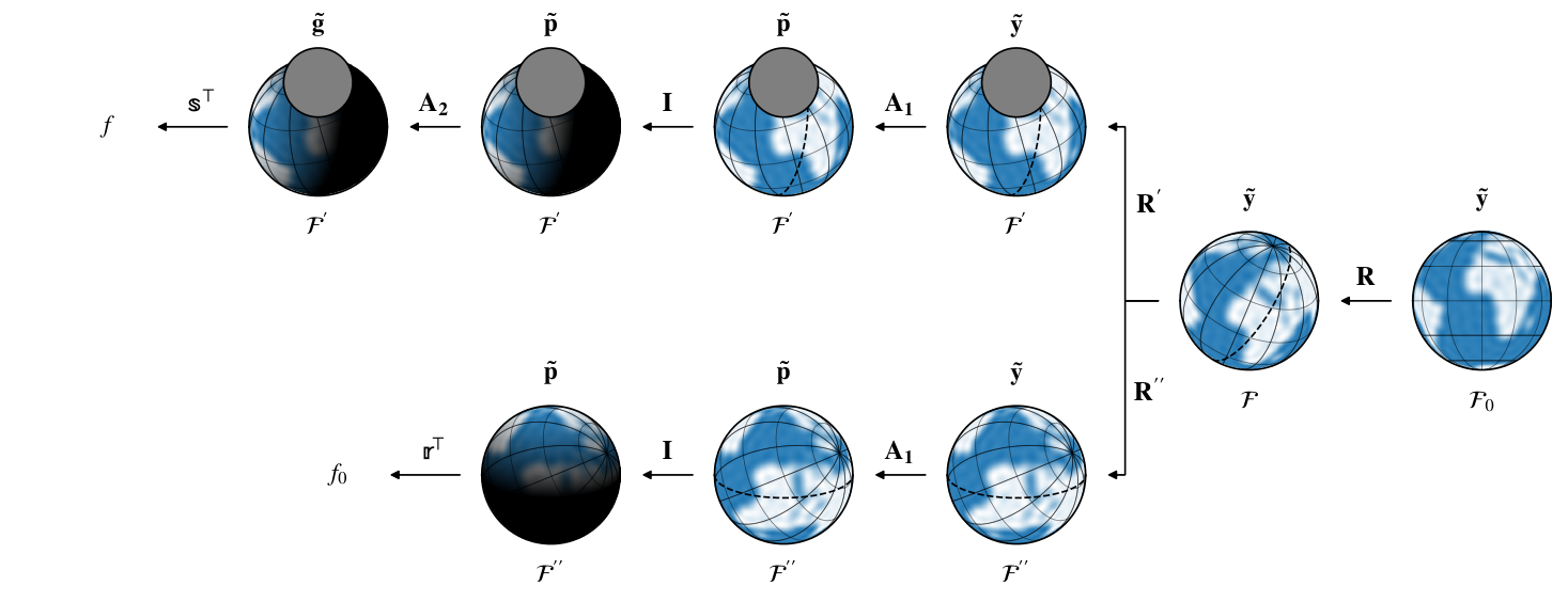
Figure 14 summarizes the transformations involved in the two equations above. Starting on the right with a map vector in the spherical harmonic basis , defined in some observer-independent frame , we first rotate it via to the sky frame , in which the body is viewed by the observer. If an occultor is present (upper branch of the figure), we rotate the map from via to the frame , in which the occultor lies along the -axis. We then apply to change basis to and to weight the map by the illumination. Finally, we change basis via to the Green’s basis, in which we compute and dot the integrals . If, on the other hand, there is no occultation (lower branch of the figure), we instead rotate the map via to the integration frame , in which the terminator is parallel to the -axis. We then apply to change basis to , apply the illumination transform , and finally dot in the solutions to the surface integrals .
Appendix B The Solution: No Occultation
Before we tackle configurations involving occultations, we must address the simpler problem of computing the total visible flux from an unocculted body in reflected light (Equation A20). This problem was originally solved by Haggard & Cowan 2018 and subsequently by Luger et al. 2019b, but for completeness we present the detailed derivation in the starry formalism here.
As we discussed above, we perform the integration in a frame in which the semi-major axis of the terminator is aligned with the -axis, with the illumination source at . The solution vector may then be computed from
| (B1) |
which is identical to Equation (20) in Luger et al. 2019a except for the lower integration limit of the inner integral. The lower limit is now the equation describing the terminator, which ensures we always exclude the nightside from the integration region. Equation (B1) may be solved analytically in terms of purely trigonometric and algebraic functions of . The component of at index is given by
| (B2) |
where the components of , , and are given by
| (B3) |
where is the gamma function.
Given initial conditions
(B4)
we may compute all the required higher order terms from the recurrence relations
| (B5) |
Once is known, the observed total flux in reflected light is computed from (c.f. Equation A20)
| (B6) |
Finally, for future reference, we can also compute what we will call the complement of case 0:
| (B7) |
This is the flux contribution from the unphysical night side (if we were to integrate over it), where our polynomial illumination (Equation A.2) function yields negative intensities. This quantity will be useful in negating the unphysical contribution in the integrals of the following section.
Appendix C The Solution: Occultation
The integration in the unocculted case presented above is relatively straightforward, since the boundaries of integration are always the half-ellipse defining the terminator and the half-circle defining the upper limb of the body (Equation B1). When an occultor is present, however, the integration boundaries are far less trivial, since they may or may not include sections of the terminator, sections of the limb of the body, and sections of the limb of the occultor. The integration regions may also be disjoint; for instance, in case 7 of Figure 15, the portion of the dayside that is unocculted consists of two separate regions.
Whereas in Luger et al. 2019a we compute the observed flux by always integrating over the unocculted portion of the disk, here we find that it is often easier and more computationally efficient to compute the integral of the intensity over the simplest region – meaning the one with the fewest boundaries – and combine it with the formalism from §B to compute the visible flux. These integrals may be over the unocculted dayside, the occulted dayside, the unocculted nightside, or the occulted nightside; in the case of the latter three, a bit of algebra (§C.3–§C.4) is needed to relate these to the observed flux. Additionally, in some cases we can avoid computing new integrals entirely, as the solution can be obtained from a combination of the classical starry solution vector and the formalism from the unocculted case (§B).
After exhaustive experimentation, we identified in total 14 families of geometrical configurations for the occultation problem, each defined by a distinct combination of integration boundaries; these are shown in Figures 15 and 17. Together, these cases encompass all possible occultation configurations, for any illumination angle, occultor size, and occultor position.
Before we discuss how to compute the occultation integrals, we must first develop a procedure to identify the relevant case given the occultor impact parameter and radius and the terminator semi-minor axis and angle in the frame . Then, once the case is determined, we must identify the relevant integration boundaries, which depend on the points of intersection between the limb of the body, the limb of the occultor, and the terminator. We do so in the following sections.
C.1 Case determination

The key to identifying the case corresponding to a given configuration is to determine whether or not the limb of the occultor intersects the terminator of the body, and if so, the points of intersection. While we perform the integration in frame , finding the points of intersection with the terminator is easier if we temporarily switch to the frame , in which the terminator is parallel to the -axis. In this frame, the equations defining the terminator and the limb of the occultor are, respectively,
| (C1) |
where
| (C2) |
are the coordinates of the occultor in . We wish to find the vector of points for which . Following Luger et al. 2017, we may express this condition as the quartic equation
| (C3) |
with coefficients
| (C4) |
Although closed-form solutions to quartic equations exist (see, e.g., Hughes & Chraibi 2011, who solve for the area of overlap between two ellipses analytically), they are prone to significant numerical instabilities. Instead, we solve for the roots of the quartic numerically by casting it as an eigenvalue problem (Edelman & Murakami 1995, e.g.,) and polish the results with a few iterations of Newton’s method. We find that this is reasonably computationally efficient and yields roots with precision within a couple orders of magnitude of machine epsilon (see §III.2).
In general, the quartic defined by Equation (C3) has (potentially degenerate) roots, some of which may be complex, and some of which correspond to intersections with the wrong half of the terminator ellipse (i.e., the section of the terminator on the far side of the body). After excluding the unphysical solutions, we are still left with anywhere between zero and four roots.
Cases with zero roots (case 1 – case 5) are treated in §C.2, while cases with one or two roots (case 6 – case 10) are treated in §C.3. Cases with three or four roots (case 11 – case 14) are rarely encountered in practice, but are possible for some pathological configurations; these are treated in §C.4.
C.2 Cases 1–5
Cases 1–5 (see Figure 15) involve configurations in which the occultor does not intersect with the terminator of the occulted body, and are therefore fairly straightforward to solve. In particular, we can use the original emitted light solution from Luger et al. 2019a, provided we weight the map by our polynomial illumination function:
| (C5) |
where is the emitted light solution vector (Luger et al. 2019a, Equation 26 in). The flux is the flux one would measure from a body whose surface map is weighted by the illumination function during an occultation. Note that this is not necessarily the observed flux, since this may include the unphysical negative contribution from the nightside. We must compute the actual observed flux on a case-by-case basis.
Case 1 corresponds to any complete occultation of the body (), so the solution for the flux is trivial:
| (C6) |
Case 2 corresponds to occultations in which the occultor blocks all of the dayside of the body and some of the nightside. In this configuration, the unocculted part of the disk consists only of nightside, so the solution is again trivial:
| (C7) |
Conversely, case 3 corresponds to occultations in which the occultor blocks all of the nightside of the body and some of the dayside. Since the visible portion of the disk consists only of dayside, we can simply use the weighted solution in emitted light (Equation C5):
| (C8) |
Case 4 involves any occultation in which the occultor blocks only the nightside of the body (regardless of whether or not it intersects with the limb of the body). Since the nightside intensity is zero everywhere, this case is also trivial, as the flux is equal to the flux in the no occultation case (Equation B6):
| (C9) |
Finally, case 5 involves any occultation in which the occultor blocks only the dayside of the body (regardless of whether or not it intersects with the limb). We first compute the illumination-weighted flux as above, then negate the unphysical nightside contribution using Equation (B7):
| (C10) |
C.3 Cases 6–10

Cases 6–10 (see Figure 15) correspond to configurations in which the limb of the occultor intersects with the terminator at either one point (case 6) or two points (cases 7–10). Because of these intersections, we cannot simply re-weight the emitted light solution, as the integration boundaries are now different. In general, we may compute the flux by integrating the components of the Green’s basis over the region bounded by three curves, which we denote , , and . These are shown in orange in Figure 15 and presented in more detail in Figure 16. Curve is a segment of the limb of the occultor, parametrized by the angle ; curve is a segment of the terminator, parametrized by the angle ; and curve is a segment of the limb of the occulted body, parametrized by the angle . The endpoints and are functions of the solutions to the quartic from §C.1 and will be presented in §C.5.
Let be the integral of over :
| (C11) |
We defer the solution to Equation (C11) to §C.5 below, as it is quite lengthy. Given , the flux over the integration region is computed from Equation (A18):
| (C12) |
Note again that this is not necessarily the observed flux, which we must compute on a case-by-case basis below.
Case 6 corresponds to configurations in which the limb of the occultor intersects the terminator at a single point. The integration region (see Figures 15 and 16) is the occulted portion of the dayside, which is bounded by all three curves , , and . The total flux may be computed by subtracting the occulted flux from the total dayside flux :
| (C13) |
Cases 7–10 involve two points of intersection between the occultor limb and the terminator. Cases 7 and 8 correspond to occultors that block some of the nightside and some of the dayside, but neither of the extrema of the terminator ellipse. In case 7 a lens-shaped region is formed by the intersection of the occultor limb and the terminator on the nightside, while in case 8 this region is formed on the dayside. In case 7, we begin by computing the flux over the unocculted region, , which includes the spurious nightside contribution. We then remove this contribution by noting that it is equal to the total nightside contribution, , minus the occulted nightside flux, :
| (C14) |
Case 8, on the other hand, is equivalent to case 6, since the integration region consists of occulted dayside:
| (C15) |
Cases 9 and 10 correspond to occultors that also block some nightside and some dayside, along with both of the extrema of the ellipse; these are therefore exclusively for large occultors (). Case 9 involves occultations in which only a small lens-shaped region of the nightside is visible. The total flux is the visible dayside plus unphysical nightside contribution, , minus the nightside contribution, which we compute from Equation (C12):
| (C16) |
Conversely, case 10 involves occultations in which only a small lens-shaped region of the dayside is visible. In this case, we may compute the observed flux from Equation (C12) directly:
| (C17) |
C.4 Cases 11–14

Cases 11–14 correspond to (rare) configurations involving three or four roots to Equation (C3) and are illustrated in Figure 17. All four involve integration over two disjoint regions (see the figure). Cases 11 and 12 involve three points of intersection between the terminator and the occultor limb. In case 11, the regions of integration and are the occulted portion of the dayside, so the solution is similar to that of cases 6 and 8:
| (C18) |
where and are computed from Equation (C12) for each of the integration regions. Conversely, in case 12 the two regions are the occulted portion of the nightside, so the solution is similar to that of case 7:
| (C19) |
Finally, cases 13 and 14 involve four points of intersection between the terminator and the occultor limb. The regions of integration in case 13 are the visible portion of the nightside, so this case is equivalent to case 9:
| (C20) |
Conversely, the regions of integration in case 14 are the visible portion of the dayside, so this case is equivalent to case 10:
| (C21) |
C.5 Computing the integrals
In the previous sections, we discussed how to identify the case corresponding to a specific configuration of the occultor and the illumination source. We showed how in some cases (1–5; §C.2) the total flux may be computed by exploiting the classical starry integrals (Equation C5). In all other cases (6–14; §C.3 and §C.4), however, the flux computation involves evaluation of Equation (C12), where the solution vector is the vector of integrals (in the frame ) of each of the terms in the Green’s basis over a region of the projected disk of the occultor (Equation C11). As in Luger et al. 2019a, the approach to computing is to use Green’s theorem to transform the surface integrals into line integrals along the curves , , and (see Figure 16). Specifically, we write22 2 In this section, we deliberately drop the dependence of and the primitive integrals on the geometrical parameters for clarity.
| (C22) |
where is a vector of two-dimensional Cartesian vectors chosen such that its exterior derivative is ,
| (C23) |
and
| (C24) |
where is the parametrized angle along the integration path and the integral is taken in a counter-clockwise direction relative to the center of the integration region. Luger et al. 2019a showed that one possible solution to Equation (C23) consists of the vector whose component is given by
| (C25) |
We showed in the previous sections that there are at most three curves , , and bounding a given closed surface of integration (see Figure 16). We may therefore express Equation (C.5) as
| (C26) |
where we define the primitive integrals33 3 The components of the vectors and are analogous to the primitive integrals and defined in Equations (30)–(32) in Luger et al. 2019a, although the integration limits of both and the sense of integration of are different.
| (C27) | ||||
| (C28) | ||||
| (C29) |
to be the line integrals of along each of the curves
, , and , respectively, where the coordinates along each
curve are parametrized
in terms of as follows:
(C30)
and we define
| (C31) |
to be the sum of definite integrals between pairs of limits arranged in a vector of length . For future reference, it will also be useful to define the operator
| (C32) |
which sums the difference of successive pairs of values in a vector . This will come in handy when computing definite integrals. Specifically, if is the antiderivative of some function , we may use the fundamental theorem of calculus to compute the integral of over the interval(s) given by the vector of limit pairs :
| (C33) |
where is the vector given by
| (C34) |
Note that most of the cases (1–10) involve integration over a single closed region, so Equations (C.5) and (C32) reduce to
| (C35) |
and
| (C36) |
For cases 11–14, we must integrate over two disjoint regions, so we sum over two pairs of limits. In the next three sections, we derive the solutions to each of the primitive integrals , , and .
C.6 The integral along the occultor limb,
In this section we present a solution to Equation (C27). The first order of business is to derive expressions for the integration limits . Depending on the integration case, these limits will correspond to the point of intersection between the limb of the occultor and the limb of the occulted body and/or the point of intersection between the limb of the occultor and the terminator of the occulted body. The former is given by (Luger et al. 2019a, c.f. Equation 24 in)
| (C37) |
where the sign is chosen such that the point is on the dayside of the occulted body, and the latter (of which there may be multiple) is given by
| (C38) |
where are the roots of the quartic (Equation C3). These angles are then wrapped to the range and sorted into the vector such that the integration is always performed in a counter-clockwise sense about the center of the integration region. The left panel in Figure 16 shows a configuration in which the lower integration limit corresponds to the point of intersection between the limbs of the two bodies and the upper integration limit corresponds to the limb-terminator intersection. Both angles are measured counter-clockwise from the line .
In order to evaluate the integral in Equation (C27), we follow the reparametrization tricks of §D.2.3 in Luger et al. 2019a. The algebra is long and tedious, so we merely present the result (alongside the usual validation links). The component of is
| (C39) |
where and we define the Vieta operator
| (C40) |
as the dot product of a vector and the vector of Vieta’s theorem coefficients, where (Luger et al. 2019a, c.f. Equation D34 in)
| (C41) |
The vectors , , , and are solutions to specific integrals, which we compute recursively below. As in Luger et al. 2019a the term of , , is handled separately; we also compute this below.
Note that several of the cases in Equation (C39) are identical to those in Equation (D35) of Luger et al. 2019a, provided we replace their integrals and with our integrals and , respectively. The integrals themselves are similar, except for a change in the limits of integration, which are no longer symmetric about zero. As we will see, this leads to the dependence of these expressions on incomplete elliptic integrals. Note also that the integrals and are new, as certain cancellations in Luger et al. 2019a resulted in the corresponding cases contributing zero net flux (Luger et al. 2019a, last case in Equation D35 of).
C.6.1 The vector
The components of the vector are given by the integral
| (C42) |
for , where we define the helper angle
| (C43) |
The integral in the expression above is the same as that in Equation (D38) of Luger et al. 2019a, except for a change in the limits of integration. As in Luger et al. 2019a, we can compute the vector recursively given a trivial lower boundary condition:
| (C44) |
where the last expression is valid for all . We find that this algorithm is generally stable, except when is small. In that limit, we evaluate by numerical integration of Equation (C42) using Gauss-Legendre quadrature with 100 points. We then recurse downward by substituting in Equation (C.6.1) and solving for .
C.6.2 The vector
The components of the vector are given by the integral
| (C45) |
where
| (C46) |
The integral in this expression is again the same as that in Equation (D39) of Luger et al. 2019a, except for a change in the limits of integration. In that paper, we computed all terms from a three-term recurrence relation and two boundary conditions. In the case of upward recursion, the boundary conditions and were computed analytically from the complete elliptic integrals and . In cases where upward recursion was not numerically stable, we evaluated and via a quickly convergent series expansion and recursed downward.
In order to solve Equation (C45), it is possible to replace the complete elliptic integrals and in the lower boundary conditions (Luger et al. 2019a, Equation D46 in ) with the incomplete elliptic integrals
| (C47) | ||||
| and | ||||
| (C48) | ||||
which we compute from the parametrization of Bulirsch 1965, then use the same upward recursion relation to obtain analytic solutions for all :
| (C49) |
where the last expression is valid for all and
| (C50) |
with
| (C51) |
Note that when we use the reciprocal-modulus transformation to evaluate the elliptic integrals:
| (C52) | ||||
| with | ||||
| (C53) | ||||
In practice, however, we find that this procedure is even more numerically unstable than it was in Luger et al. 2019a. To address this, we express the recurrence structure of the problem as a tridiagonal system with one lower boundary condition and one upper boundary condition :
| (C54) |
where the recursion coefficients are given by
| (C55) |
Solving this matrix system yields values for all intermediate . While efficient algorithms exist for solving tridiagonal problems, we obtain far better numerical stability by instead performing traditional LU decomposition. We find that this algorithm is stable in all the regimes that we tested.
We evaluate the upper boundary condition by numerical integration of Equation (C45) via Gauss-Legendre quadrature with 100 points. While the lower boundary condition may be computed analytically from Equation (C.6.2), in practice we achieve better precision via numerical integration (as above), with negligible effects on computational performance.
C.6.3 The vector
C.6.4 The vector
The components of the vector are given by the integral
| (C58) |
We may compute it by either upward or downward recursion. In both cases, we compute each of the from
| (C59) |
In the upward case, we start with the lower boundary conditions
| (C60) |
and recurse upward in and simultaneously:
| (C61) |
for . In the case of downward recursion, we start with the upper boundary conditions
| (C62) |
where
| (C63) |
and is the Gauss hypergeometric function, which we compute via its series definition. We recurse downward in and simultaneously:
| (C64) |
C.7 The term
The final integral we must solve is that corresponding to (). As in Luger et al. 2019a, this is the integral of the linear limb darkening term, whose solution must be handled separately due to the fact that the corresponding antiderivative in Equation (C25) is not a polynomial in , , and ; also see Agol et al. 2020. The integral we must solve is
| (C65) |
where is the usual Cartesian coordinate (Equation A6). The solution is tricky, but fortunately a similar integral was solved in Equation (34) of Pál 2012. Adapting their solution to our formalism, we obtain
| (C66) |
where
| (C67) | ||||
| and | ||||
| (C68) | ||||
The quantities and are the same incomplete elliptic integrals as those in §C.6.2, while
| (C69) |
is the incomplete elliptic integral of the third kind, with
| (C70) |
While stable algorithms exist to evaluate (Bulirsch 1969, e.g.), we find that the parametrization above has poor numerical stability, particularly in the vicinity of the singular points and . In practice, we find that numerical evaluation of Equation (C65) via Gaussian quadrature is more numerically stable and just as computationally efficient as the procedure outlined above.
C.8 The integral along the terminator,
In this section we present a solution to Equation (C28), the line integral along the day/night terminator of the occulted body. As before, the first thing we must do is derive expressions for the integration limits . Depending on the integration case, these limits will corresponds to the point of intersection between the terminator and the limb of the occultor and/or the point of intersection between the terminator and the limb of the occulted body. The former is given by
| (C71) |
where are the roots of the quartic (Equation C3). The latter is given by
| (C72) |
As before, these angles are then wrapped to the range and sorted into the vector such that the integration is performed counter-clockwise about the center of the integration region. The middle panel of Figure 16 shows a case where corresponds to the point of intersection between the occultor limb and the terminator and corresponds to the point where the terminator extends onto the backside of the body. Note, importantly, that unlike , the angle is not measured between the horizontal and a point on the curve of . Recall that is an angular parameter of the ellipse, so it is measured in the same way as the eccentric anomaly in a Keplerian orbit: it is the angle between the semi-major axis of the ellipse and the perpendicular projection of a point on the ellipse onto the unit circle (see Figure 16).
The solution to Equation (C28) involves repeated application of the binomial theorem. If we define the quantities
| and | ||||
| (C73) | ||||
we may express the solution to the integral as
The solution to Equation (C74) depends on the matrix , whose components are given by the integral
| (C75) |
The integral is the same as that in Equation (D27) of Luger et al. 2019a, except for a change in the limits of integration. We can compute this integral recursively given four lower boundary conditions:
| (C76) |
The remaining terms may be computed by upward recursion using the relations
| (C77) |
for and
| (C78) |
for all remaining terms.
C.9 The integral along the occulted body limb,
The final line integral we must solve is the integral along the boundary of the occulted body, Equation (C29). Fortunately, this is also the easiest of the three. The limits of integration correspond to the point at which the terminator crosses from the dayside to the night side,
| (C79) |
and the point of intersection between the limb of the occultor and the limb of the occulted body,
| (C80) |
where the sign is chosen such that the point is on the dayside of the occulted body. As before, these angles are wrapped to the range and placed in the vector such that the line integral is taken in the counter-clockwise direction about the center of the integration region. The right panel of Figure 16 shows a case where and . Both angles are measured counter-clockwise from the -axis.
Appendix D Caveats
The starry code includes a large suite of unit tests that compare the flux computations to numerical models and to various benchmarks for a wide variety of inputs. While we have done our best to develop tests over the full range of occultation configurations, there may be edge cases in which the starry algorithm fails and returns the wrong flux. This could happen, for instance, if the quartic root solver (§C.1) fails to find the points of intersection between the occultor and the day/night terminator, leading to an incorrect case identification (Figure 15) and thus the wrong value for the flux. In the development of the algorithm, these cases would occasionally show up as a single, obvious outlier in a light curve model. All such cases we encountered have been fixed by adding consistency checks in the root solver and switching to alternate evaluation methods near known singularities. However, it is possible that there may still be rare cases in which this happens, in which case we ask that users raise an issue on GitHub so that we can provide a fix.
| Symbol | Description | Reference |
|---|---|---|
| Frames of reference | ||
| frame in which surface map is specified | §A.1 | |
| observer (sky) frame | §A.1 | |
| integration frame (occultor present) | §C | |
| integration frame (no occultor) | §B | |
| Lines & surfaces | ||
| region of integration enclosed by | §C | |
| integration path along occultor limb | §C | |
| integration path along body limb | §C | |
| integration path along terminator | §C | |
| Special functions | ||
| arctan2 | quadrant-aware arctangent | (A10) |
| incomplete elliptic integral of the first kind | (C47) | |
| Gauss hypergeometric function | §C.6.4 | |
| incomplete elliptic integral of the second kind | (C48) | |
| gamma function | §B | |
| incomplete elliptic integral of the third kind | (C69) | |
| Operators & symbols | ||
| Vieta summation operator | (C40) | |
| pairwise difference operator | (C32) | |
| vectorized integral | (C.5) | |
| Symbol | Description | Reference |
|---|---|---|
| Integers | ||
| spherical harmonic degree | (A.1) | |
| spherical harmonic order | (A.1) | |
| vector index | — | |
| spherical harmonic index, | (A.1) | |
| spherical harmonic index, | (A.1) | |
| Coordinates | ||
| Cartesian coordinate on the plane of the sky | — | |
| Cartesian coordinate on the plane of the sky | — | |
| Cartesian coordinate, | (A6) | |
| Geometrical parameters | ||
| semi-minor axis of terminator ellipse | (A9) | |
| complement of , | §A.2 | |
| occultor impact parameter, | §A.1 | |
| elliptic parameter | (C46) | |
| I | body inclination | §A.1 |
| elliptic characteristic | (C70) | |
| occultor radius | §A.1 | |
| distance to illumination source, | §A.2 | |
| occultor position | §A.1 | |
| illumination source position | §A.2 | |
| occultor position | §A.1 | |
| illumination source position | §A.2 | |
| illumination source position | §A.2 | |
| body obliquity | §A.1 | |
| angle of rotation of the terminator ellipse | (A19), (A21) | |
| body rotational phasse | §A.1 | |
| Intensities & fluxes | ||
| orbital semi-major axis | §IV.1 | |
| albedo (spherical) | (1) | |
| reflected flux during an occultation | §C | |
| reflected flux outside of an occultation | (B6) | |
| complement of reflected flux outside of an occultation | (B7) | |
| – | case-dependent reflected flux during occultation | §C |
| intensity-weighted flux during an occultation | (C5) | |
| thermal flux during an occultation | (A3) | |
| thermal flux outside of an occultation | (A7) | |
| reflected flux over integration region | (C12) | |
| polynomial intensity at a point on the surface | (A.2) | |
| true intensity at a point on the surface | (A11) | |
| planet radius | §IV.1 | |
| stellar radius | §IV.1 | |
| polar angle of incidence | Figure 9 | |
| polar angle of reflection | Figure 9 | |
| Oren-Nayar surface roughness coefficient | §IV.2 | |
| Angular extent of terminator past | (4) | |
| azimuthal angle of incidence | Figure 9 | |
| azimuthal angle of reflection | Figure 9 | |
| Symbol | Description | Reference |
|---|---|---|
| Bases | ||
| Green’s basis | (A4) | |
| polynomial basis | (A8) | |
| spherical harmonic basis | (A1) | |
| Angles & angular parameters | ||
| cosine-like parameter of | (C51) | |
| modified angle along occultor limb | (C43) | |
| angle along occulted body limb | §C.9 | |
| angle along occultor limb | §C.6 | |
| angle along terminator | §C.8 | |
| Integrals | ||
| unocculted solution in emitted light | §A.1 | |
| occultation solution in emitted light | §A.1 | |
| helper integral | (C42) | |
| helper integral | (C45) | |
| helper integral | (B) | |
| primitive integral | (C27) | |
| primitive integral | (C29) | |
| unocculted solution in reflected light | (B1) | |
| occultation solution in reflected light | (C26) | |
| primitive integral | (C28) | |
| helper integral | (C56) | |
| helper integral | (C58) | |
| Other vector quantities | ||
| vector of albedo values on a discrete surface grid | (12) | |
| data vector | §V.1 | |
| vector of flux values | §V.1 | |
| illumination profile in polynomial basis | (A15) | |
| solution to quartic in terminator frame | (C3) | |
| vector of spherical harmonic coefficients | §A.1 | |
| prior mean | §V.1 | |
| Symbol | Description | Reference |
|---|---|---|
| Linear operators | ||
| change of basis matrix: | §A.1 | |
| change of basis matrix: | §A.1 | |
| change of basis matrix: | §A.2 | |
| posterior covariance matrix | §V.1 | |
| illumination operator | (A17) | |
| pixelization operator | (12) | |
| inverse pixelization operator | (14) | |
| rotation matrix: | §A.1 | |
| rotation matrix: | §A.1 | |
| rotation matrix: | §A.1 | |
| starry design matrix | §V.1 | |
| prior covariance matrix | §V.1 | |
| data covariance matrix | §V.1 | |
| Integrals | ||
| anti-exterior derivative of | (C25) | |
| helper integral | (C75) | |
| helper integral | (B) | |
| helper integral | (B) | |
| Symbol | Description | Value |
|---|---|---|
| If is this close to , compute in the limit | ||
| If or are less than this value, set to this value | ||
| If is within this value of unity, nudge it away | ||
| If is less than this value, nudge away from | ||
| If is within this amount of , nudge it away | ||
| If is within this amount of , nudge it away | ||
| If is less than this value, set to this value | ||
| If is within this value of zero, nudge it away | ||
| If is within this amount of , nudge it away | ||
| If two quartic roots are this close, eliminate one of them | ||
| If is within this value of unity, set it to unity | ||
| If is within this amount of when , nudge it away |