( e = e 0 ) ∨ ( e 0 = ∅ ) e ⊢ ( c a , ⟨ Δ 1 , p c 2 ⟩ ) ↪ ⟨ Δ 2 , p c 2 ⟩
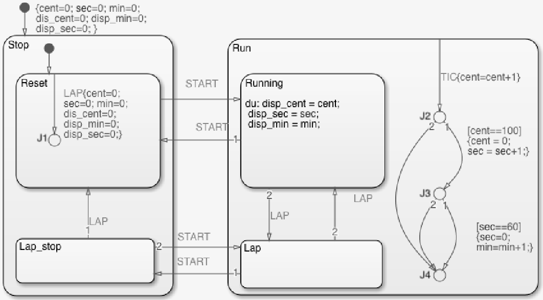
e ⊢ ( ( e 0 , c , c a , t a , d ) , ⟨ Δ 1 , p c 1 ⟩ ) → ⟨ Δ 2 , p c 2 ⟩ , F i r e ( d , t a ) ‾ The [t-FIRE] rule for both SOS and SSOS semantics is shown in Figure 2(a) and Figure 2.2 , respectively. The rule describes how a Stateflow transition fires, and intuitively it captures the following: in the concrete execution, if the evaluation of a condition evaluates to true ( ⊤ ), and the execution of the condition action c a modifies the environment, then a Stateflow program performs a transition, and raises a Fire transition value. In Figure 2.2 , we show an SSOS counter-part of the [t-FIRE] rule to visually illustrate the similarities and differences of the rules side-by-side. An intuitive explanation for the rule is given in Section .
For the complete set of SOS rules, we refer the interested reader to the original work by Hamon and Rushby [hamon2004operationalsemanticsstateflow , hamon2007operationalsemanticsstateflow ] .
2.3 Satisfiability Modulo Theories and Z3
The problem of determining whether a Boolean formula can be made true by assigning truth values to the constituent Boolean variables is known as the Boolean satisfiability problem (SAT). A decision procedure for SAT is a procedure that generates a (satisfying) assignment for the variables for which a given formula is true, whenever the formula is satisfiable. Satisfiability Modulo Theories (SMT) represents an extension of SAT, where some of the logic symbols are interpreted by a background theory [barrett18smtbookchapter ] . An example of such a background modulo-theories are the theory equality, theory of integer numbers, theory of real numbers, etc.
Z3 [demoura08z3 ] is a state of the art SMT solver and theorem prover developed by Microsoft Research. The input is a model specified in a text-based assertion language that follows the SMT-LIB standard [barret15smtlib ] . Z3 provides a number of APIs for different programming languages, including C and Python, which enables the integration of the Z3 solver with other applications. The input model consists of a set of variables of specific types (also called sorts), and a set of assertions that express constraints over the variables. The basic command called assert is used to add an assertion to the internal stack of the solver. Once the stack is loaded with the set of assertions of interest, the satisfiability of the constraints is checked by the check-sat command. There are 3 possible outcomes from the decision procedure: sat which indicates that there exists an assignment of the variables satisfying the set of assertions, unsat indicating that there does not exist such a satisfying assignment, and unknown when the decision procedure cannot determine the satisfaction of the assertions on the stack.
2.4 Bounded Model Checking
In this section, we give an overview of the Bounded Model Checking (BMC) technique, which we use for checking invariant properties of Stateflow programs.
BMC is a refutation-based verification technique, in which a symbolic representation of the system behavior is unrolled for a predefined number
k of steps, called the reachability diameter . It has been shown that checking a property over a finite set of states can be reduced to checking the satisfiability of a corresponding propositional formula. Thus, the goal of BMC is to generate a formula that is satisfiable if there exists a violation of the property in some execution of length up to k . The reduction of the model-checking problem to a satisfiability problem is motivated by the increase in the computational power of modern solvers, which tend to be more efficient in solving large formulas as compared to techniques based on BDDs [demoura03BMCrefutationtoverification ] .
To be able to formally define the BMC problem for invariant properties, we first recall some additional background concepts. A common way of capturing program behavior is via a transition system (TS), formally defined as follows.
Definition 1 (Transition System).
A transition system is a tuple 𝑇𝑆 = ( C , C 0 , → ) C configurations , C 0 ⊆ C initial configurations , and → ⊆ C × C transition relation .
Let π π = c 0 , c 1 , … , c n π = c 0 , c 1 , c 2 … π
•
a path of 𝑇𝑆 , written path( π ), if ∀ c i , c i + 1 ∈ π . ( c i , c i + 1 ) ∈ → , and
•
an initialized path , if path( π ) and c 0 ∈ C 0 .
A finite path π = c 0 , c 1 , … , c n length n
Transition systems are a useful concept for reasoning about the concrete computations of programs. A configuration c ∈ C of a program is a pair c = ( l , v ) , where l is a control point in the program, and v is a mapping between the program variables and values taken from their respective domains.
When programs contain variables that range over infinite domains, it can be more efficient to reason about their behaviors in a symbolic way, through a set of predicates. This gives rise to the notion of symbolic transition system (STS).
Definition 2 (Symbolic Transition System).
A symbolic transition system is a pair S = ( I , R ) I ( ⋅ ) R ( ⋅ , ⋅ )
I ( c ) ⇔ c ∈ C 0
R ( c , c ′ ) ⇔ ( c , c ′ ) ∈ →
Every initialized path in S of length k can be characterized by the formula:
and then, the existence of an initialized path of length k is equivalent to the satisfiability of the formula 𝑝𝑎𝑡ℎ ( x 0 , x 1 , … , x k ) , where x i is a variable representing a configuration.
Since BMC operates over a subset of the reachable configurations, contained within the given reachability diameter k , in this work we use the term k to denote an invariant property that holds over the reachability diameter k .
Let φ be a unary predicate over configurations, i.e., a property. We define the corresponding k -bounded invariant property, denoted φ k , as the formula:
To disprove such a k -bounded invariant property, it is sufficient to show that there exists a configuration within the reachability diameter for which φ k does not hold. A path containing such a configuration is called a counter-example , and is characterized by the logical negation of the above formula, i.e.:
Given that the predicates I , R , and φ can be expressed as FOL formulas, where some function and predicate symbols are potentially interpreted by some background theory, it is obvious how the refutation of k -bounded invariant properties can be reduced to an SMT problem. In case that there exists a satisfying assignment for ( ), a counter-example for the invariant property is generated. Conversely, if there exists no such satisfying assignment, the k -bounded invariant property holds.
3 Symbolic Structural Operational Semantics
In this section, we present our SSOS semantics for the Stateflow imperative language, which we use as a basis for constructing an STS
S ^ for a given Stateflow program. We start from the existing SOS semantics as in [hamon2004operationalsemanticsstateflow , hamon2007operationalsemanticsstateflow ] , and transform each of the SOS rules uniformly in a corresponding symbolic counterpart.
From earlier (see Section 2.1 ), we know that the SOS rules for Stateflow programs are over judgments of the following form:
Based on the set of SOS rules, one can induce a T S = ( C , C 0 , → ) , where C is the set of concrete configurations, each configuration c ∈ C being a tuple c = ( P , D ) , C 0 ⊆ C is the set of initial configurations, and → ⊂ C × C is the transition relation, composed of transitions derivable by the SOS rules.
In the original formalization, the sets of variables ( 𝑉𝑎𝑟 ) and values ( 𝑉𝑎𝑙 ), as well as the sets of actions ( 𝐴𝑐𝑡 ) and conditions ( 𝐶𝑜𝑛𝑑 ) are considered to be a part of the action language which is distinct from the Stateflow language itself. The details for the actions and conditions are abstracted away; however, it is assumed that the semantics of the executing actions and the evaluating conditions is available via judgments of the form:
which are read as follows: (i) evaluating an action ( a ) in a current environment ( D ) produces a new environment ( D ′ ), and (ii) evaluating a condition ( c ) in an environment ( D ) produces either true or false Boolean value.
The set of SSOS rules is created by uniformly transforming each of the SOS rules into a corresponding symbolic rule, by: i) replacing each valuation of the program variables, called environment ( D ) with a symbolic representation ( Δ ), and ii) adding a path condition ( 𝑝𝑐 ). Consequently, we update the action execution and condition evaluation, which evaluate over the symbolic environment and path condition, respectively. Following the basic principles of symbolic execution [king1976symbolicexecutionandtesting ] , in the set of SSOS rules we treat the data component of the language in a symbolic way, whereas the control-flow remains concrete.
As we already discussed in Section , the set of all initialized paths of length k of a Stateflow program can be symbolically encoded as formulas. In such a representation, the analysis operates over sets of environments, rather than with each environment individually. Conceptually, Δ represents a set of concrete environments that is characterized by a path formula that includes all concrete environments reachable at a particular point of execution, while 𝑝𝑐 represents the path condition that encodes the conditions over data such that Δ is valid.
Figure 2 : Illustrative sample of SSOS rules. We define a symbolic configuration 𝑠𝑐 ∈ 𝑆𝐶 as a structure ( P , ⟨ Δ , 𝑝𝑐 ⟩ ) , where P is any component from the imperative language from Table 1 . We introduce a new set of symbolic variables (symbols), denoted 𝑆𝑦𝑚 , and a bijection g : 𝑉𝑎𝑟 → 𝑆𝑦𝑚 between the program variables and the symbols. The path condition p c is simply a Boolean expression over the set of symbols, whereas the symbolic environment Δ ∈ 𝑆𝐸𝑛𝑣 is a mapping Δ : 𝑉𝑎𝑟 → 𝐸𝑥𝑝𝑟 𝑆𝑦𝑚 from program variables to (arithmetic) expressions over symbols. Finally, we assume that symbolic action execution and symbolic condition evaluation are provided via semantic functions of type 𝒮 𝒜 : 𝐴𝑐𝑡 → ( 𝑆𝐸𝑛𝑣 → 𝑆𝐸𝑛𝑣 ) and 𝒮 ℬ : 𝐶𝑜𝑛𝑑 → ( 𝑆𝐸𝑛𝑣 → 𝐵𝐸𝑥𝑝𝑟 𝑆𝑦𝑚 ) , respectively.
We can now define the axioms for action execution and condition evaluation, for symbolic execution of Stateflow programs, as follows:
e ⊢ ( a , ⟨ Δ 1 , p c 1 ⟩ ) ↪ ⟨ Δ 2 , p c 1 ⟩ if Δ 2 = 𝒮 𝒜 [ [ a ] ] ( Δ 1 ) (4)
e ⊢ ( c , ⟨ Δ 1 , p c 1 ⟩ ) → ⟨ Δ 1 , p c 2 ⟩ if p c 2 = p c 1 ∧ 𝒮 ℬ [ [ c ] ] ( Δ 1 )
The initial symbolic configuration is ( P , ⟨ p c 0 , Δ 0 ⟩ ) , where P is a component of the Stateflow imperative language, Δ 0 = g , and p c 0 = ⊤ .
The set of SOS rules can now be uniformly translated into a corresponding SSOS counter-part. In Figure , we show a subset of the SSOS rules, in addition to the [t-FIRE] rule from Figure 2.2 .
The [t-FIRE] rule in Figure 2.2 describes how a Stateflow transition ( t ) fires by appending the symbolic evaluation of the condition t . c to the current path condition and by symbolically executing the condition action t . c a over the current symbolic environment Δ . When a transition fires, a transition event F i r e ( t . d , t . t a ) is generated. Going back to Figure , a transition list T fires via the [T-FIRE] rule when one of its constituent transitions fires. The [SD-FIRE] rule describes how a Stateflow state fires when one of the transitions from the T o transition list fires. According to the rule, the firing of the transition is followed by symbolic evaluation of the pending action from the existing F i r e event, then symbolic execution and evaluation of the actions and conditions of the currently active inner component(s), and finally the symbolic evaluation of the s d . e x state action. The last two rules, [AND] and [OR-FIRE] capture the correct sequence of elements processing when executing the And and Or- compositions, respectively. Executing an And- composition involves processing each of its constituent states from the state definition list ( S D ), whereas an Or- composition fires when the underlying s d fires. Due to space limitations, Figure shows only a small fraction of the rules for illustrative purposes. The complete set of 27 SSOS rules is included in Appendix .
Since we are overloading the transition relation symbol “ → ” in the SOS and SSOS rules, to avoid confusion, further in the paper we shall use “ → 𝑆𝑂𝑆 ” for transitions derivable with the SOS rules, and “ → 𝑆𝑆𝑂𝑆 ” for transitions derivable with the SSOS rules.
4 Characterization of the SSOS
Our SSOS semantics is essentially an operational semantics for symbolic execution of Stateflow programs. It opens up the opportunity for application of a broader spectrum of verification techniques, such as: testing (purely symbolic, or as a combination of symbolic and concrete (concolic) testing [godefroid05dartconcolictesting ] ) or bounded model checking [biere2003boundedmodelchecking ] . To be able to reason symbolically over Stateflow programs, however, one must first provide a formal characterization of the relationship between its concrete and symbolic execution. In this section, we prove two results that characterize this relationship. In Theorem
First, we introduce some additional notation.
Let
β : 𝑆𝐸𝑛𝑣 × 𝐸𝑛𝑣 → 𝐸𝑛𝑣 be a function that transforms a symbolic environment Δ into a concrete one β ( Δ , D ) with the help of an environment D that serves as an interpretation of the symbolic values; for any v ∈ V a r , let β ( Δ , D ) ( v ) be defined as the value of the expression Δ ( v ) in the (renamed) environment D ∘ g − 1 .
Similarly, let ℬ : 𝐵𝐸𝑥𝑝𝑟 𝑆𝑦𝑚 → ( 𝐸𝑛𝑣 → 𝐵𝑜𝑜𝑙 ) be a function that evaluates path conditions in concrete environments, so that ℬ [ [ 𝑝𝑐 ] ] ( D ) is the Boolean value of the path condition 𝑝𝑐 in D ∘ g − 1 .
Finally, observing that the transitions derived by the SSOS rules only (potentially) add a conjunct to the current path condition p c k to obtain a new path condition p c k + 1 , let p c k k + 1 denote this added conjunct (or ⊤ , if no conjunct is added).
Theorem 1 .
If ( P 1 , ⟨ Δ 1 , p c 1 ⟩ ) → S S O S ( P 2 , ⟨ Δ 2 , p c 2 ⟩ , t v ) D 0 ∈ 𝐸𝑛𝑣 ℬ [ [ p c 1 2 ] ] ( β ( Δ 1 , D 0 ) ) = ⊤ ( P 1 , β ( Δ 1 , D 0 ) ) → S O S ( P 2 , β ( Δ 2 , D 0 ) )
Proof.
For proving the result, we shall use the principle of Rule Induction (see, e.g., [winskel1993formalsemanticsofprogramminglanguages , p. 41] ).
The principle states that, in order to prove that a given predicate over judgements holds for all judgements derivable by a given set of rules, one has to show that every rule preserves the predicate. In the statement of the theorem, the predicate to be proved is the one defined by the then-clause.
The complete proof has thus to consider each of the 27 rules of the SSOS. We include here only a few selected cases of the proof to illustrate the proof technique. As it can be seen from the given cases, all of them follow the same pattern, so it should be clear to the reader how the complete proof unfolds.
Case 1.1. [t-FIRE] SSOS Since the two premises of the rule are not transitions over which the statement is proved, we can treat them as side conditions and assume them to be true (since otherwise one cannot apply the rule).
Next, let D_0 ∈ Env b e s u c h t h a t :
(5)
Equation 5
5
B
[
[
c
]
]
(
β
(
Δ
1
,
D
0
)
)
=
⊤
a n d l e t D_1, D_2 ∈Env . D_1 = β (Δ_1, D_0) a n d D_2 = β (Δ_2, D_0) . T h e n , w e h a v e e ⊢(c, D_1) →D_1 a n d e ⊢ (a, D_1) → D_2 , a n d t h e r e f o r e e ⊢(t, D_1) →D_2, Fire(d, ta) , w h e r e pc_2 = pc_1 ∧ c a n d Δ_2 = SA [[a]](Δ_1) . T h e p r e m i s e s o f t h e [ t − F i r e ] SOS r u l e a r e t h u s t r u e , a n d w e c a n a p p l y t h e r u l e t o o b t a i n t h e f o l l o w i n g :
⊢
e
→
(
t
,
D
1
)
D
2
,
F
i
r
e
(
d
,
t
a
)
w h i c h i s w h a t n e e d e d t o b e d e m o n s t r a t e d . Case 1.2 [T-FIRE] SSOS L e t D_0 ∈ Env , a n d t = t.T b e s u c h t h a t :
(6)
Equation 6
6
B
[
[
t
.
c
]
]
(
β
(
Δ
1
,
D
0
)
)
=
⊤
a n d l e t D_1, D_2 ∈ Env . D_1=β(Δ_1, D_0), D_2=β(Δ_2, D_0) . F r o m ( ) , a n d t h e i n d u c t i o n h y p o t h e s i s i t f o l l o w s :
(7)
Equation 7
7
e
,
⊢
J
→
(
t
,
D
1
)
D
2
,
Fire
(
d
,
ta
)
N o w t h a t t h e p r e m i s e f o r [ T − F I R E ] SOS r u l e g i v e n i n ( ) i s t r u e , w e c a n a p p l y t h e r u l e t o o b t a i n t h e f o l l o w i n g :
e
,
J
⊢
(
t
.
T
,
D
1
)
→
D
2
,
Fire
(
d
,
ta
)
w h i c h c o n c l u d e s t h e p r o o f f o r t h e c a s e . Case 1.3 [SD-FIRE] SSOS L e t D_0 ∈ Env b e s u c h t h a t :
(8)
Equation 8
8
B
[
[
p
c
1
2
]
]
(
β
(
Δ
1
,
D
0
)
)
=
⊤
,
B
[
[
p
c
2
3
]
]
(
β
(
Δ
3
,
D
0
)
)
=
⊤
,
B
[
[
p
c
3
4
]
]
(
β
(
Δ
4
,
D
0
)
)
=
⊤
w h e r e pc_2 = pc_1 ∧ pc_1^2, pc_3 = pc_2 ∧ pc_2^3, pc_4 = pc_3 ∧ pc_3^4 . B a s e d o n ( ) , w e k n o w t h a t
∃
D
1
,
…
,
∈
D
5
E
n
v
.
D
1
=
β
(
Δ
1
,
D
0
)
,
D
2
=
β
(
Δ
2
,
D
0
)
,
D
3
=
β
(
Δ
3
,
D
0
)
,
=
D
4
β
(
Δ
4
,
D
0
)
,
=
D
5
β
(
Δ
5
,
D
0
)
F r o m ( ) a n d t h e i n d u c t i o n h y p o t h e s i s , i t f o l l o w s t h a t :
(9)
Equation 9
9
e
,
⊢
J
0
→
(
T
0
,
D
1
)
D
2
,
F
i
r
e
(
d
,
t
a
)
;
⊢
e
→
(
a
,
D
2
)
D
3
;
e
,
J
⊢
(
C
,
D
3
)
→
D
4
;
e
,
J
⊢
(
A
.
e
x
,
D
4
)
→
D
5
S i n c e t h e p r e m i s e s f o r [ S D − F I R E ] SOS r u l e g i v e n i n ( ) a r e t r u e , w e c a n a p p l y t h e r u l e t o o b t a i n t h e f o l l o w i n g :
e
,
⊢
J
O
→
(
(
A
,
C
,
T
i
,
T
o
,
J
)
,
D
1
)
(
(
A
,
C
′
,
T
i
,
T
o
,
J
)
,
D
5
)
,
F
i
r
e
(
d
,
⋄
)
w h i c h i s w h a t n e e d e d t o b e s h o w n . Case 1.4 [AND] SSOS L e t D_0 ∈Env b e s u c h t h a t t h e f o l l o w i n g h o l d s :
(10)
Equation 10
10
∀
i
∈
[
1
,
…
,
n
]
.
B
[
[
p
c
i
+
i
1
]
]
(
β
(
Δ
i
,
D
0
)
)
=
⊤
;
F r o m t h e i n i t i a l a s s u m p t i o n a n d ( ) , w e k n o w t h a t :
∈
∀
k
[
1
,
…
,
+
n
1
]
.
∈
∃
D
k
Env
.
=
D
k
β
(
Δ
k
,
D
0
)
F r o m t h e i n d u c t i o n h y p o t h e s i s a n d ( ) , i t f o l l o w s t h a t :
(11)
Equation 11
11
∈
∀
i
[
1
,
…
,
n
]
e
,
⊢
J
→
(
sd
i
,
D
i
)
sd
i
′
,
D
+
i
1
,
No
S i n c e t h e p r e m i s e f o r t h e [ A N D ] SSOS r u l e ( ) i s t r u e , w e c a n a p p l y t h e r u l e t o o b t a i n t h e f o l l o w i n g :
⊢
e
,
J
(
e
,
J
⊢
(
A
n
d
{
s
0
:
s
d
0
⋯
s
n
:
s
d
n
}
,
D
1
)
→
(
A
n
d
{
s
0
:
s
d
′
0
⋯
s
n
:
s
d
′
n
}
,
D
+
n
1
,
N
o
)
w h i c h i s w h a t w a s n e e d e d t o b e s h o w n . Case 1.5 [OR-FIRE] SSOS L e t D_0 ∈Env b e s u c h t h a t t h e f o l l o w i n g h o l d s :
(12)
Equation 12
12
B
[
[
p
c
1
2
]
]
(
β
(
Δ
1
,
D
0
)
)
=
⊤
;
B a s e d o n ( ) , t h e f o l l o w i n g h o l d s :
∈
∃
D
1
,
D
2
Env
.
=
D
1
β
(
Δ
1
,
D
0
)
,
=
D
2
β
(
Δ
2
,
D
0
)
F r o m t h e i n d u c t i v e h y p o t h e s i s a n d ( ) , i t f o l l o w s t h a t :
(13)
Equation 13
13
e
,
⊢
J
→
(
sd
,
D
1
)
(
sd
′
,
D
2
)
,
Fire
(
p
′
,
a
)
S i n c e t h e p r e m i s e f o r t h e [ O R − F I R E ] SOS r u l e ( ) i s t r u e , w e c a n a p p l y t h e r u l e t o o b t a i n t h e f o l l o w i n g :
⊢
e
,
J
(
O
r
(
s
,
p
,
T
,
S
D
[
s
:
s
d
]
)
,
D
1
,
t
v
)
→
(
O
r
(
∅
s
,
p
,
T
,
S
D
[
s
:
s
d
′
]
)
,
D
2
,
F
i
r
e
(
p
′
,
a
)
)
w h i c h i s w h a t w a s n e e d e d t o b e s h o w n . ∎ O u r n e x t r e s u l t e s t a b l i s h e s t h e r e v e r s e d i r e c t i o n .
Theorem 2
Theorem 2
2
Theorem 2
Theorem 2.
If
S
O
S
→
(
P
1
,
D
1
)
(
P
2
,
D
2
)
, then for all
∈
p
c
1
BExpr
Sym
,
∈
Δ
1
SEnv
and
∈
D
0
Env
such that
=
β
(
Δ
1
,
D
0
)
D
1
, there exist
p
c
2
,
∈
p
c
1
2
BExpr
Sym
and
∈
Δ
2
SEnv
such that
=
p
c
2
∧
p
c
1
p
c
1
2
,
B
[
[
p
c
1
2
]
]
(
β
(
Δ
1
,
D
0
)
)
=
⊤
,
=
β
(
Δ
2
,
D
0
)
D
2
and
S
S
O
S
→
(
P
1
,
⟨
Δ
1
,
p
c
1
⟩
)
(
P
2
,
⟨
Δ
2
,
p
c
2
⟩
)
.
Proof.
Again , theproofisbyRuleInduction . Weonlyshowtwocaseshere . Therestofthecasesareprovedbyfollowingtheschemeofthepresentedones
Case 2.1. [t-FIRE] SOS LetusassumethataStateflowprogramperformsaconcretetransitionderivableusingthe [ t − Fire ] SOS rule . Letsassumethatforarbitrary ⟨ Δ 1 , 𝑝𝑐 1 ⟩ ∈ 𝑆𝑆 the following holds:
Also, we know that 𝑝𝑐 1 2 = ℬ [ [ c ] ] ( β ( Δ 1 , D 0 ) ) = ⊤ , due to the inductive hypothesis. Consequently, the following also holds: ℬ [ [ 𝑝𝑐 1 ∧ c ] ] ( β ( Δ 1 , D 0 ) ) = ⊤ . Based on ( ) and the true valuation of 𝑝𝑐 1 ∧ c , the following also holds:
where 𝑝𝑐 2 = 𝑝𝑐 1 ∧ c and Δ 2 = 𝒮 𝒜 [ [ a ] ] ( Δ 1 ) . Based on ( ) and the induction hypothesis we derive the following: e ⊢ ( c , ⟨ Δ 1 , 𝑝𝑐 1 ⟩ ) → ⟨ Δ 1 , 𝑝𝑐 2 ⟩ and e ⊢ ( a , ⟨ Δ 1 , 𝑝𝑐 2 ⟩ ) → ⟨ Δ 2 , 𝑝𝑐 2 ⟩ . If we now apply the [t-Fire] SSOS rule over the last two premises, we derive the following transition:
which is what needed to be demonstrated.
Case 2.2 [T-FIRE] SOS Let us assume that a Stateflow program performs a concrete transition derivable using the [T-Fire] SOS rule. Let us assume that for an arbitrary ⟨ Δ 1 , pc 1 ⟩ ∈ SS the following holds:
Also, we know that pc 1 2 = ℬ [ [ c ] ] ( β ( Δ 1 , D 0 ) ) = ⊤ , due to the inductive hypothesis. Consequently, the following also holds: ℬ [ [ pc 1 ∧ c ] ] ( β ( Δ 1 , D 0 ) ) = ⊤ . Based on ( ) and the truth valuation of the pc 1 ∧ c , the following also holds:
where pc 2 = pc 1 ∧ c and Δ 2 = 𝒮 𝒜 [ [ a ] ] ( Δ 1 ) . Based on ( ) and the induction hypothesis we derive the following: e ⊢ ( c , ⟨ Δ 1 , pc 1 ⟩ ) → ⟨ Δ 1 , pc 2 ⟩ and e ⊢ ( a , ⟨ Δ 1 , pc 2 ⟩ ) → ⟨ Δ 2 , pc 2 ⟩ . If we now apply the [T-Fire] SSOS rule over the last two premises, we derive the following transition:
which is what needed to be demonstrated.
∎
There are two important corollaries of the above two results, which we will only state here informally. First, both results lift naturally to executions , i.e., to sequences of transitions. Note in particular how in Theorem the “for all 𝑝𝑐 1 …there exists 𝑝𝑐 2 ” part allows the sequential composition of transitions. Second, when starting from a true path condition, as one does in symbolic execution, the satisfying assignments for the path condition at the end of any symbolic path, viewed as interpreting environments, define precisely the concrete paths that follow the symbolic one.
Further, the executions in SOS and SSOS can be shown to simulate each other with respect to processing external events. It is well-known that invariant properties are preserved by simulation, and thus, can be checked by symbolically executing the given Stateflow program.
Even if limited, this class of properties is important in industrial contexts, as our collaboration with Scania on formally verifying safety-critical embedded code generated from Simulink models has shown.
5 From Stateflow Programs to SMT Solving
In our work, we focus on using BMC for checking invariant properties over symbolic representation of Stateflow programs. In Section k-bounded invariant checking problem for the latter representation (Section
5.1 Bounded Invariant Checking for Stateflow Programs
In this section, we define a version of STS that encode the symbolic behaviors of Stateflow programs, and then adapt the BMC problem to such transition systems.
Definition 3 (STS over Symbolic Configurations).
A symbolic transition system over the symbolic configurations of a given Stateflow program is an STS S ^ = ( I ^ , R ^ )
I ^ ( ⋅ ) and R ^ ( ⋅ , ⋅ ) are thus a unary “initialization” predicate and a binary “next-state” predicate over the symbolic configurations of the program, respectively, which are quantifier-free FOL formulas over the components of symbolic configurations.
The formal relationship between an STS over symbolic configurations S ^ and an ordinary STS S of a Stateflow program is given by the following result.
Proposition 1 .
Let SF be a Stateflow program, S = ( I , R ) S ^ = ( I ^ , R ^ )
Proof.
Direction ( ⇒ ) of (1) . Assume that I ^ (P, ⟨Δ, pc⟩) = ⊤ . F r o m t h e d e f i n i t i o n o f i n i t i a l s y m b o l i c c o n f i g u r a t i o n ( S e c t i o n ) , w e k n o w t h a t t h a t pc = pc_0 a n d Δ= Δ_0 , a n d t h a t pc_0 = ⊤ a n d Δ= g . S i n c e pc = ⊤ , t h e r e m u s t e x i s t D_0 ∈Env s u c h t h a t I(P, D_0) , a n d β (Δ, D_0) = D . G i v e n t h a t Δ= g , i t f o l l o w s t h a t D = D_0 . S i n c e I(P, D_0) = ⊤ , t h e n a l s o I(P, D) = ⊤
Direction ( ⇐ ) of (1 ).
A s s u m e t h a t t h e r e e x i s t s D_0 ∈Env s u c h t h a t I(P, D_0) , B [[pc]]( β (Δ, D_0)) = ⊤ , a n d I(P, β (Δ, D_0)) . I f I(P, β (Δ, D_0)) = ⊤ , t h e n β (Δ, D_0) = D . I(P, D_0) = ⊤ a n d I(P, D) = ⊤ i f a n d o n l y i f D = D_0 . T h i s i s p o s s i b l e o n l y i f Δ= g . G i v e n t h e d e f i n i t i o n o f i n i t i a l s y m b o l i c c o n f i g u r a t i o n ( S e c t i o n ) , t h e a s s u m p t i o n B [[pc]]( β (Δ, D_0)) = ⊤ , a n d Δ= g , i t f o l l o w s t h a t I ^ (P, ⟨Δ, pc⟩) = ⊤
Direction ( ⇒ ) of (2).
A s s u m e t h a t R ^ ((P, ⟨Δ_1, pc_1⟩), (P’, ⟨Δ_2, pc_2 ⟩)) = ⊤ . A c c o r d i n g t o D e f i n i t i o n 3 , i f R ^ ((P, ⟨Δ_1, pc_1 ⟩), (P’, ⟨Δ_2, pc_2 ⟩)) = ⊤ , t h e n t h e r e e x i s t s (P, ⟨Δ_1, pc_1 ⟩) → SSOS (P’, ⟨Δ_2, pc_2 ⟩) . F r o m T h e o r e m 1 , i f (P, ⟨Δ_1, pc_1 ⟩) → SSOS (P’, ⟨Δ_2, pc_2 ⟩) , t h e n f o r a l l D_0 ∈Env s u c h t h a t B [[pc_1]]( β (Δ_1, D_0)) = ⊤ , a n d B [[pc_1^2]]( β (Δ_1, D_0)) = ⊤ , t h e r e i s (P, β (Δ_1, D_0)) → SOS (P, β (Δ_2, D_0)) . U s i n g t h e r e s u l t f o r t h e e x i s t e n c e o f a n S O S t r a n s i t i o n , a n d D e f i n i t i o n 2 , w e c a n c o n c l u d e t h a t :
R
(
(
P
,
β
(
Δ
1
,
D
0
)
)
,
(
P
,
β
(
Δ
2
,
D
0
)
)
)
=
⊤
A s s u m e t h a t t h e r e e x i s t s D_0 ∈Env s u c h t h a t B [[pc_1]]( β (Δ_1, D_0)) = ⊤ , B [[pc_2]]( β (Δ_2, D_0)) = ⊤ , a n d R((P, β (Δ_1, D_0)), (P’, β (Δ_2, D_0))) = ⊤ . F r o m D e f i n i t i o n 2 , i f R((P, β (Δ_1, D_0)), (P, β (Δ_2, D_0))) = ⊤ , t h e n (P, β (Δ_1, D_0)) → SOS (P, β (Δ_2, D_0)) . B a s e d o n t h e e x i s t e n c e o f (P, β (Δ_1, D_0)) → SOS (P, β (Δ_2, D_0)) , a n d b y f o l l o w i n g T h e o r e m 2 , w e h a v e t h a t f o r a l l pc_1 ∈BExpr_Sym , Δ_1 ∈SEnv , a n d D_0 ∈Env s u c h t h a t β (Δ_1, D_0) = D_1 , t h e r e e x i s t pc_1^2, pc_2 ∈BExpr_Sym , a n d Δ_2 ∈SEnv s u c h t h a t pc_2 = pc_1 ∧pc_1^2 , B [[pc_1^2]]( β (Δ_1, D_0)) = ⊤ , β (Δ_2, D_0) = D_2 a n d (P, ⟨Δ_1, pc_1⟩) → SSOS (P’, ⟨Δ_2, pc_2⟩) . U s i n g t h e r e s u l t f o r t h e d e r i v e d S S O S t r a n s i t i o n , a n d D e f i n i t i o n 3 , w e c a n c o n c l u d e t h a t R ^ ((P, ⟨Δ_1, pc_1⟩), (P’, ⟨Δ_2, pc_2⟩)) = ⊤ . ∎ N o w , l e t φ b e a p r e d i c a t e o v e r t h e c o n c r e t e c o n f i g u r a t i o n s o f a S t a t e f l o w p r o g r a m . P r e d i c a t e φ i n d u c e s a c o r r e s p o n d i n g p r e d i c a t e φ ^ (sc) ≜ φ (sc[g^-1]) o v e r t h e s y m b o l i c c o n f i g u r a t i o n s sc = (P, ⟨ pc, Δ ⟩ ) , w h e r e g i s t h e b i j e c t i o n f r o m S e c t i o n . A s s u m i n g a n i n t e r p r e t a t i o n f o r t h e p a t h a n d k − b o u n d e d i n v a r i a n t p r o p e r t y f o r m u l a s f o r e x e c u t i o n s o v e r s y m b o l i c c o n f i g u r a t i o n s , t h e c o u n t e r − e x a m p l e p a t h f o r m u l a ( ) f o r s y m b o l i c e x e c u t i o n s c a n b e r e w r i t t e n a s f o l l o w s :
(16)
Equation 16
16
∃
s
c
0
,
…
,
s
c
k
.
(
∧
p
a
t
h
(
s
c
0
,
…
,
s
c
k
)
⋁
=
i
0
k
¬
^
φ
(
s
c
i
)
)
B a s e d o n f o r m u l a ( ) , a n d a l o n g t h e l i n e s o f t h e d e f i n i t i o n o f B M C f o r C p r o g r a m s g i v e n i n [armando2009smt-bmc ] , w e d e r i v e t h e f o l l o w i n g .
Theorem 3
Theorem 3
3
Theorem 3
Theorem 3.
Let SF be a Stateflow program,
=
^
S
(
^
I
,
^
R
)
be an STS over its symbolic configurations, and
φ
k
be a k-bounded invariant property. Then, the following two statements are equivalent:
1.
item 1
1
item 1
SF satisfies the k-bounded invariant property
φ
k
.
2.
item 2
2
item 2
The formula
∧
p
a
t
h
(
s
c
0
,
…
s
c
k
)
⋁
=
i
0
k
¬
^
φ
(
s
c
i
)
is UNSAT.
Proof.
( Bycontradiction . ) AssumethatagivenStateflowprogramdoesnotsatisfythe k − boundedinvariantproperty φ k , and that statement (2) holds. From the definition of k -bounded invariant property, we know that such a property fails if there exists a path in which the last configuration violates φ . From Definition , we know that such a path exists if the formula given in (2) is satisfiable (SAT), which contradicts the initial assumption.
Assume that the formula in (2) is SAT, and that the statement (1) holds. The satisfiability of the formula says that there exists a reachable state sc i . i < k , in which the negation of the property φ ^ holds, that is, φ ^ ( sc i ) = ⊤ . In such case φ ^ k is not an invariant, which contradicts our initial assumption.
∎
Now that we have formally defined BMC invariant checking for STS over symbolic configurations, we show how to construct the predicates I ^ and R ^ for a given Stateflow program.
5.2 From Stateflow Programs to SMT Scripts
In this section, we describe a procedure for deriving an STS from a given Stateflow program using the set of SSOS rules, and the transformation of the STS predicates into quantifier-free FOL formulas that can be used for k-bounded invariant checking over symbolic configurations, as defined in Theorem
S ^ = ( I ^ , R ^ ) from a given Stateflow program, one must make a decision as to the granularity of the transitions in executions. At its highest syntactic level, any Stateflow program is an Or -composition or an And -composition. Since our running example is an Or -composition, and since conceptually the procedure for And -compositions is virtually the same, in the following we focus on the Or -compositions only. We derive an STS in which the transitions between configurations correspond to transitions at the top Or -composition level. Due to the layered structure of the imperative language, each such transition consists of a series of transitions at the lower levels (see Table 1 from Section 2.2 ). Our approach to the derivation of the top-level transitions is to use our SSOS to perform symbolic execution between any possible pair of consecutive control points of the program, for arbitrary values of the data. One should note that in general case, the derivation of the STS is not strictly bound to the top-level component, as it can be done against any syntactic class of the Stateflow imperative language.
As a result of our adopted modeling principle, the configurations for the induced STS are of the following type: ( Or , ⟨ pc , Δ ⟩ ) . Even though the program component during execution remains the same (the top-level Or -component), it can be the case that its internal configuration changes. The internal configuration of an Or -component is characterized by the set of active substates. Consequently, the program control points correspond to the possible internal configurations at the top Or -composition level.
For instance, our running Stateflow example from Figure 1 has 5 program control points, namely: i) no active states, ii) Stop and Reset , iii) Stop and Lap_stop , iv) Run and Running , and v) Run and Lap .
One way of modeling the program control points as defined above is to extend the set of variables 𝑉𝑎𝑟 with a set of auxiliary Boolean variables ( 𝑉𝑎𝑟 C ). For every control point 𝑂𝑟 , the set of variables 𝑉𝑎𝑟 C can be partitioned into two subsets: the set 𝑉𝑎𝑟 C + = { v | v ∈ 𝑉𝑎𝑟 C , v = ⊤ } corresponding to the active states of 𝑂𝑟 , and 𝑉𝑎𝑟 C − = 𝑉𝑎𝑟 C ∖ 𝑉𝑎𝑟 C + . Thus, the control point 𝑂𝑟 is characterized by the formula:
The initial symbolic configuration for an STS of a Stateflow program given as an Or -composition is defined as ( Or ∅ , ⟨ pc 0 , Δ 0 ⟩ ) , where: Or ∅ is an uninitialized Or -component that has no active substates, pc 0 = ⊤ , and Δ = g (see Section ). As explained, in our STS we only have transitions between symbolic configurations of the form ( 𝑂𝑟 , ⟨ 𝑝𝑐 , Δ ⟩ ) → ( 𝑂𝑟 ′ , ⟨ 𝑝𝑐 ′ , Δ ′ ⟩ ) , where Or and Or ′ are consecutive program control points. To express the predicates I ^ and R ^ as quantifier-free FOL formulas, we need to construct the quantifier-free FOL formulas for the pc and Δ components of the symbolic configurations.
The path condition pc is a quantifier-free Boolean expression over symbols, and as such can be viewed as a quantifier-free FOL formula Φ pc . The symbolic environment Δ , on the other hand, is a mapping between program variables and arithmetic expressions over symbols. From Δ , one can construct a quantifier-free FOL formula modulo theory of arithmetic for Φ Δ , as follows:
where 𝑉𝑎𝑟 D = 𝑉𝑎𝑟 ∖ 𝑉𝑎𝑟 C .
Now that we have defined the construction of quantifier-free FOL formulas for each of the components of the symbolic configurations of an STS, we can construct, for any transition T i between symbolic configurations, a quantifier-free FOL formula ( Φ T i ) modulo theory of arithmetic, as follows:
Finally, based on the formula ( ) and Proposition 1, we encode the predicates I ^ and R ^ as the following quantifier-free FOL modulo theory of arithmetic formulas:
I ^ ≜ Φ 𝑂𝑟 ∅ ∧ Φ Δ 0 (20)
R ^ ≜ ⋀ T i ∈ T Φ T i
where T is the set of all derivable SSOS transitions from the initial top-level composition. One way of computing T is to start from the initial program control point ( Or ∅ ) and derive all transitions between reachable program control points with a standard breadth-first or depth-first search algorithm.
The remaining step now is to encode the FOL formulas corresponding to the I ^ and R ^ predicates into the SMT-LIB script format, in order to be used as an input to an SMT-solver. We assume that the program data ( 𝑉𝑎𝑟 D ) in the Stateflow program is composed of scalar variables, which are either numeric or Boolean. There are two ways of encoding the numeric variables for SMT: i) using the theory of bit-vectors [ganesh07bitvector ] , or ii) directly as variables of the sort that corresponds to their numeric domain. The bit-vector encoding provides an accurate way of capturing the binary representation of the numeric values; however, the resulting formula depends on the size of the vector. The numeric representation, on the other hand, provides an encoding independent of the binary representation, but does not guarantee completeness for non-linear arithmetic expressions. In our case, the latter suffices. We model the events using Boolean variables.
An earlier work shows how a sequence of C commands can be converted into an SMT script [armando2009smt-bmc ] , using the concepts of conditional normal form , and single static assignment form (SSA) (see, e.g., [cytron1989ssa ] ). A program is in conditional normal form if all the statements are of the form if (c) then r , where r is either an assertion or an assignment. The SSA encoding principle requires each variable to be assigned only once, which means that for each assignment a fresh variable is added to the set 𝑉𝑎𝑟 . For instance, v 1 1 is a fresh variable that represents the first intermediate assignment of the variable v during the second execution step. This resolves the SMT-encoding for the sequential execution of the accumulated actions from the derived transitions.
6 Practical Evaluation of SESf
In this section, we present the preliminary results from the initial practical evaluation of our approach (henceforth referred to as SESf ). As benchmark, we use the Stopwatch running example from Section 2.1 1
To this date, we have automated the following aspects of our approach: the generation of an underlying STS
S ^ = ( I ^ , R ^ ) , the incremental unrolling of the predicate R ^ that models the program execution, and checking the satisfiability of the generated formula after each unrolling, using the Z3 solver. The only part that is not yet automated is the SMT-LIB encoding of the underlying STS.
Before we delve into the analysis, we explain the environmental setup for the evaluation. Our SESf tool requires that the Stateflow model is encoded into the imperative language, which is then provided as an input to the SESf tool. As the transformation of the graphical model into an imperative program is beyond the scope of this paper, we assume that there exists a tool that converts an original Stateflow model into a program written in the imperative language. The complete evaluation is performed on a standard MacBook Pro workstation with a 2,4 GHz Quad-Core Intel Core i5 processor and 8GB of RAM memory. We use Matlab version R2020b.
The set T of symbolic transitions at the program level is generated by a symbolic execution engine which is implemented in Python. For each of the transitions, the symbolic execution engine generates a certificate for the correctness of the transition in the form of an SSOS derivation tree [sesfGitLink ] . The tool generates the set T for the Stopwatch program, consisting of 22 transitions, within one second. Next, we manually encode the set T into SMT-LIB assertions, by following the procedure described in Section .
Figure 3 : Evaluation results Next, we proceed to the main part of the evaluation, where we measure the time required by the tool to find a violation for a given invariant property, i.e., a counter-example, which is completely automated. In order to test the time for finding a counter-example, we analyze the Stopwatch model against the following parametric invariant property: The value of cent is always between 0 and X , for which we know that there exists a counter-example trace of a specific length since the cent variables will increase up to 100. We then run the analysis for the following set of values for X : { 5 , 10 , 20 , 40 , 80 , 99 } . The SESf was able to provide a counter-example for each instance of the property. The results, in terms of time required to find the counter-example for each of the values of X , are given in Figure .
Following the data plot, we can see that the SESf tool was able to find violation for all the parameter values for the parametric safety property in a time frame ranging from several seconds to less than two minutes. Even though the obtained data can be best judged in a head-to-head comparison with the state-of-the-practice tool for formal verification of Stateflow models, we are unable to do so due to the aforementioned licensing issues. In spite of the limited validation presented in this section, we deem our approach and the prototype implementation to have potential for practical application as it was able to find the injected design errors within a reasonable time frame.
7 Related Work
To the best of our knowledge, the present work is the first to define a symbolic operational semantics for any kind of Stateflow language, and a corresponding notion of STS over symbolic configurations. The main goal of this paper has been to establish the foundations for provably correct verification of Stateflow models using symbolic methods, while the development of a practical tool and its extensive evaluation has mostly been left as future work. Still, in this section we will outline some of the state-of-the-art approaches and tools for the formal analysis and verification of Stateflow models, and will draw some high-level parallels to our work.
The most common way of formally verifying Stateflow models is to propose and apply transformation rules for the basic Stateflow modeling constructs into some existing formal framework. Yang et al. [yang16stateflowtransformationase , jiang2019dependablecpsstateflow ] propose a technique for transforming Stateflow models into Uppaal timed automata. The main idea of the technique is that by translating a Stateflow model into a timed automaton one creates a timed model, which can then be subjected to verification with respect to timing and liveness properties, based on an informal semantics of the Stateflow language. A similar endeavour is by Chen [chen10formalanalysisofstateflowdiagrams ] , where an approach for formal analysis of Stateflow diagrams based on the PAL model checker is presented. Although claimed by the author that all of the Stateflow modeling principles are covered, the correctness of the formal model cannot be formally demonstrated. Meenakshi et al. [meenakshi2006toolfortranslatingsimulink ] propose a tool for the transformation of Simulink models into the input language of a model checker. Similarly to the previous work, the main limitation of this work is proving the correctness of the transformation. Miyazawa et al. [miyazawa12refinementorientedmodelsofstateflow ] provide a formalization of Stateflow in a refinement language called Circus. The main difference with our work lies in the fact that the they define formal semantics specific for the Circus language, whereas in our case the semantics are defined in generalized SOS-style. The consequence of this is the usability of the semantics, which in the case of Miyazawa et al. [miyazawa12refinementorientedmodelsofstateflow ] are tool-specific, whereas in our case the proposed SSOS are not particularly bounded to any verification method or tool.
There exists a set of approaches that treat Stateflow models as hybrid system models, and apply corresponding modelling and analysis approaches. In this category, we can mention the approach by Alur et al. [alur2008symbolicanalysisforcoveragesimulinkstateflow ] , which uses a combination of numerical simulation and symbolic analysis for Simulink/Stateflow models for improving the simulation coverage of the models. At the core of their technique lies a transformation of Simulink/Stateflow models into linear hybrid systems , which are then used for the analysis of the models using backward image computation, in order to identify classes of inputs, which can then be analyzed using minimal numerical simulations. Zuliani et al. [zuliani10bayesiansimulinkstateflow ] employ statistical model checking (SMC) based on Bayesian statistics to reason about the correctness of Stateflow models. By resorting to SMC they alleviate the state-space explosion problem of complex Stateflow models; however, the obtained results are in a form of probabilistic bounds, which cannot be directly applied for refining the Stateflow models. Duggirala et al. [duggirala15c2e2 ] propose the C2E2 tool, which can be used for verification of a broad class of hybrid and dynamic system models based on validated simulations. In contrast, the aim of our work is to establish the foundations for a symbolic analysis of completely discrete-time Stateflow models.
There is a body of work that is focused on defining a denotational semantics for Stateflow models. Hamon [hamon2005denotational ] proposed a denotational semantics for the Stateflow imperative language, as a complement to the already existing SOS semantics, in order to formalize the compilation of Stateflow programs. The denotational semantics is particularly useful for code generation from Stateflow models. In later work, Bourbouh et al. [bourbouh2017automatedanalysisofstateflowmodels , bourbouh2020cocosim ] extended and upgraded the denotational semantics of Hamon, and employed it for the compilation of Stateflow models into hierarchical state machines, and later also into Lustre models, for SMT-based formal analysis and verification, as well as for code generation. As this approach is very similar to ours, we aim to perform in the future a more detailed comparison, especially in terms of the generated analysis model as it is generated based on a different type of semantics. Auto-Gene [toom06geneauto ] is an open-source toolset intended for code generation from high level modelling languages, including Simulink and Stateflow. The aim of the toolset is to use among others Simulink and Stateflow as input languages, from which it will automatically generate C code. It uses only a safe subset of the Simulink/Stateflow language in order to be able to provide support for the verification of properties such as termination, context independence, etc.
8 Conclusion
We presented a technique for symbolic analysis of Stateflow programs with respect to invariant properties using bounded model checking (BMC). To this end, we developed a symbolic structural operational semantics (SSOS) for the Stateflow language. Our semantics is built on top of the work by Hamon and Rushby [hamon2004operationalsemanticsstateflow , hamon2007operationalsemanticsstateflow ] , by converting each of their rules, in a uniform manner, into a symbolic form. We characterized the relationship between the two semantics by exhibiting a simulation relation between them. Next, we defined the bounded invariant checking problem for STS over symbolic configurations, as induced for a given Stateflow program by the set of the SSOS operational rules, and presented informally a procedure for deriving the initial and next state predicates of the STS. Finally, we showed how to generate, from the STS, a set of quantifier-free FOL assertions in SMT-LIB format suitable for analysis using state-of-the-art SMT solvers. The main benefit of our work is that it lays down the foundations for
the development of tools for the scalable verification of complex industrial Stateflow models by means of existing symbolic techniques, which we demonstrated with bounded invariant checking on the running Stateflow program example for different values of the depth bound k . We showed that even though in its current state the tool cannot exhaustively verify Stateflow models, it still represents a viable choice for fast detection of design errors within a traces of finite length. Even though we initially planned to compare our approach against the state-of-the-practice SLDV tool, we had to withdraw from our idea once we discovered the license constraints imposed by Mathworks. Unfortunately, this happened in the final stage of this work, when it was already too late to steer the validation into a different direction.
Currently, we are working on automating the remaining parts of our technique, and packaging it into a user-friendly and easy to use tool-set. Our goal is to fully automate the transformation of the Stateflow programs into a symbolic representation, to be used as input to (bounded) invariant checkers, either applied to Stateflow programs in isolation, or as part of already existing frameworks for symbolic analysis of Simulink models (see, e.g., [filipovikj2019boundedinvariancechecking ] ). Once we have fully developed the tool-set, we will perform a more extensive evaluation of the approach, and compare its performance with that of state-of-the-art tools implementing alternative verification techniques.
Further, we plan to extend our formal characterization of the SSOS in terms of a stronger equivalence between the concrete and symbolic representations of Stateflow programs, to formally underpin the symbolic verification of a wider class of properties than invariant properties, such as LTL properties. Finally, we will explore the possibility of extending our BMC approach from refutation-based to a verification one, by adding induction [demoura03BMCrefutationtoverification ] . Along this line of research, we plan to include the option of converting the generated STS into an input format for tools that implement more sophisticated model checking algorithms, such as Lustre [pilaud1987lustre ] models for the Kind2 model checker [champion16kind2 ] .
Acknowledgements.
This work has been funded by the Swedish Governmental Agency for Innovation Systems (VINNOVA) under the AVerT project 2018-02727. The authors would also like to thank Gustav Ung for his valuable comments and constructive feedback.
References
[1]
I. The MathWorks, “Matlab&Simulink - Stateflow User’s Guide,” https://www.mathworks.com/help/pdf_doc/stateflow/stateflow_ug.pdf , The
MathWorks, Inc., 3 Apple Hill Drive Natick, MA 01760-2098, March 2020,
[Online; accessed: August 11, 2026].
[2]
D. Harel, “Statecharts: A Visual Formalism for Complex Systems,” Science of Computer Programming , vol. 8, no. 3, pp. 231–274, 1987.
[3]
I. The MathWorks, “Matlab&Simulink - Simulink User’s Guide,” https://www.mathworks.com/help/pdf_doc/simulink/simulink_ug.pdf , The
MathWorks, Inc., 3 Apple Hill Drive Natick, MA 01760-2098, March 2020,
[Online; accessed: August 11, 2026].
[4]
ISO, “Road vehicles – Functional safety,” 2011.
[5]
G. Hamon, “Simulink Design Verifier - Applying Automated Formal Methods to
Simulink and Stateflow,” in Third Workshop on Automated Formal
Methods , 2008, invited paper.
[6]
J.-F. Etienne, S. Fechter, and E. Juppeaux, “Using simulink design verifier
for proving behavioral properties on a complex safety critical system in the
ground transportation domain,” in Complex Systems Design &
Management . Springer, 2010, pp.
61–72.
[7]
P. A. Abdulla, J. Deneux, G. Stlmarck, H. Ågren, and O. Åkerlund,
“Designing safe, reliable systems using scade,” in International
Symposium On Leveraging Applications of Formal Methods, Verification and
Validation . Springer, 2004, pp.
115–129.
[8]
G. Hamon and J. Rushby, “An Operational Semantics for Stateflow,” in International Conference on Fundamental Approaches to Software
Engineering . Springer, 2004, pp.
229–243.
[9]
——, “An Operational Semantics for Stateflow,” International
Journal on Software Tools for Technology Transfer , vol. 9, no. 5-6, pp.
447–456, 2007.
[10]
G. Hamon, “A Denotational Semantics for Stateflow,” in Proceedings
of the 5th ACM international conference on Embedded software , 2005, pp.
164–172.
[11]
H. Bourbouh, P.-L. Garoche, C. Garion, A. Gurfinkel, K. Temesghen, and
X. Thirioux, “Automated Analysis of Stateflow Models,” 2017.
[12]
Y. Yang, Y. Jiang, M. Gu, and J. Sun, “Verifying Simulink Stateflow Model:
Timed Automata Approach,” in Proceedings of the 31st IEEE/ACM
International Conference on Automated Software Engineering , ser. ASE
2016. New York, NY, USA: ACM, 2016,
pp. 852–857. [Online]. Available: http://doi.acm.org/10.1145/2970276.2970293
[13]
Y. Jiang, H. Song, Y. Yang, H. Liu, M. Gu, Y. Guan, J. Sun, and L. Sha,
“Dependable Model-driven Development of CPS: From Stateflow Simulation to
Verified Implementation,” ACM Transactions on Cyber-Physical
Systems , vol. 3, no. 1, p. 12, 2019.
[14]
C. Banphawatthanarak, B. H. Krogh, and K. Butts, “Symbolic Verification of
Executable Control Specifications,” in Proceedings of the 1999 IEEE
International Symposium on Computer Aided Control System Design (Cat. No.
99TH8404) . IEEE, 1999, pp. 581–586.
[15]
C. Baier and J.-P. Katoen, Principles of Model Checking (Representation
and Mind Series) . The MIT Press,
2008.
[16]
A. Biere, A. Cimatti, E. M. Clarke, O. Strichman, Y. Zhu et al. ,
“Bounded Model Checking.” Advances in Computers , vol. 58,
no. 11, pp. 117–148, 2003.
[17]
J. C. King, “Symbolic Execution and Program Testing,” Communications
of the ACM , vol. 19, no. 7, pp. 385–394, 1976.
[18]
C. Barrett and C. Tinelli, Satisfiability Modulo Theories . Cham: Springer International Publishing, 2018.
[Online]. Available: https://doi.org/10.1007/978-3-319-10575-8_11
[19]
C. Barrett, P. Fontaine, and C. Tinelli, “The SMT-LIB Standard: Version
2.5,” Department of Computer Science, The University of Iowa, Tech. Rep.,
2015, available at www.SMT-LIB.org .
[20]
L. De Moura and N. Bjørner, “Z3: An Efficient SMT Solver,” in Proceedings of the Theory and Practice of Software, 14th International
Conference on Tools and Algorithms for the Construction and Analysis of
Systems , ser. TACAS’08/ETAPS’08. Berlin, Heidelberg: Springer-Verlag, 2008, pp. 337–340. [Online]. Available: http://dl.acm.org/citation.cfm?id=1792734.1792766
[21]
L. De Moura, H. Rueß, and M. Sorea, “Bounded Model Checking and
Induction: From Refutation to Verification,” in International
Conference on Computer Aided Verification . Springer, 2003, pp. 14–26.
[22]
P. Filipovikj, D. Gurov, and M. Nyberg, “Bounded Invariant Checking for
Stateflow Programs,” vol. abs/1207.0016, 2012.
[23]
P. Godefroid, N. Klarlund, and K. Sen, “Dart: Directed automated random
testing,” SIGPLAN Not. , vol. 40, no. 6, p. 213–223, Jun. 2005.
[Online]. Available: https://doi.org/10.1145/1064978.1065036
[24]
G. Winskel, The Formal Semantics of Programming Languages: an
Introduction . MIT press, 1993.
[25]
A. Armando, J. Mantovani, and L. Platania, “Bounded Model Checking of
Software Using SMT Solvers Instead of SAT Solvers,” International
Journal on Software Tools for Technology Transfer , vol. 11, no. 1, pp.
69–83, 2009.
[26]
V. Ganesh and D. L. Dill, “A Decision Procedure for Bit-Vectors and
Arrays,” in Proceedings of the 19th International Conference on
Computer Aided Verification , ser. CAV’07. Berlin, Heidelberg: Springer-Verlag, 2007, p. 519–531.
[27]
R. Cytron, J. Ferrante, B. K. Rosen, M. N. Wegman, and F. K. Zadeck, “An
Efficient Method of Computing Static Single Assignment Form,” in Proceedings of the 16th ACM SIGPLAN-SIGACT symposium on Principles of
programming languages , 1989, pp. 25–35.
[28]
P. Filipovikj, “SESf tool,” https://github.com/predragf/sesf , 2021,
[Online; accessed: August 11, 2026].
[29]
C. Chen, “Formal Analysis for Stateflow Diagrams,” in 2010 Fourth
International Conference on Secure Software Integration and Reliability
Improvement Companion , 2010, pp. 102–109.
[30]
B. Meenakshi, A. Bhatnagar, and S. Roy, “Tool for Translating Simulink Models
into Input Language of a Model Checker,” in International Conference
on Formal Engineering Methods . Springer, 2006, pp. 606–620.
[31]
A. Miyazawa and A. Cavalcanti, “Refinement-oriented Models of Stateflow
Charts,” Science of Computer Programming , vol. 77, no. 10-11, pp.
1151–1177, 2012.
[32]
R. Alur, A. Kanade, S. Ramesh, and K. Shashidhar, “Symbolic Analysis for
Improving Simulation Coverage of Simulink/Stateflow Models,” in Proceedings of the 8th ACM International Conference on Embedded
Software , 2008, pp. 89–98.
[33]
P. Zuliani, A. Platzer, and E. M. Clarke, “Bayesian Statistical Model
Checking with Application to Simulink/Stateflow Verification,” in Proceedings of the 13th ACM international conference on Hybrid systems:
computation and control , 2010, pp. 243–252.
[34]
P. S. Duggirala, S. Mitra, M. Viswanathan, and M. Potok, “C2E2: A
Verification Tool for Stateflow Models,” in International Conference
on Tools and Algorithms for the Construction and Analysis of Systems . Springer, 2015, pp. 68–82.
[35]
H. Bourbouh, P.-L. Garoche, T. Loquen, É. Noulard, and C. Pagetti,
“Cocosim, a code generation framework for control/command applications an
overview of cocosim for multi-periodic discrete simulink models,” in 10th European Congress on Embedded Real Time Software and Systems (ERTS
2020) , 2020.
[36]
A. Toom, T. Naks, M. Pantel, M. Gandriau, and I. Wati, “Gene-Auto: an
Automatic Code Generator for a safe subset of Simulink/Stateflow and
Scicos,” in Embedded Real Time Software and Systems (ERTS2008) ,
Toulouse, France, Jan. 2008. [Online]. Available: https://hal.archives-ouvertes.fr/hal-02270306
[37]
P. Filipovikj, G. Rodriguez-Navas, and C. Seceleanu, “Bounded Invariance
Checking of Simulink Models,” in Proceedings of the 34th ACM/SIGAPP
Symposium on Applied Computing . ACM,
2019, pp. 2168–2177.
[38]
D. Pilaud, N. Halbwachs, and J. Plaice, “LUSTRE: A Declarative Language for
Programming Synchronous Systems,” in Proceedings of the 14th Annual
ACM Symposium on Principles of Programming Languages (14th POPL 1987). ACM,
New York, NY , vol. 178, 1987, p. 188.
[39]
A. Champion, A. Mebsout, C. Sticksel, and C. Tinelli, “The Kind 2 Model
Checker,” in International Conference on Computer Aided
Verification . Springer, 2016, pp.
510–517.
Appendix A Complete Set of SSOS Rules
Figure 4 : SSOS rules for transitions.
In this appendix, we present the complete set of SSOS rules. The rules are divided in 5 categories, as follows: rules for transitions (Figure And- compositions (Figure Or- compositions (Figure
The set of SSOS rules for transitions is composed of 3 rules and is given in Figure
t fires by appending the symbolic evaluation of the condition t . c to the current path condition and by symbolically executing the condition action t . ca over the current symbolic environment Δ . When a transition fires, a transition event Fire ( t . d , t . ta ) is generated. The [t-NOT-ENABLED] rule is applicable when the event of the currently processed transition does not match the currently active event. Finally, the last rule [t-NO-FIRE] describes how a Stateflow transition does not fire because its guard does not evaluate to true. The processing of such transitions results in a new path condition, which is generated by appending the negation of the transition condition to the current path condition, while the symbolic environment remains the same.
Figure 5 : SSOS rules for transition list (part 1). Next comes the set of SSOS rules for transitions lists T , which is given in Figure . The list is composed of 7 rules, as follows. [T- ∅ ] describes how an empty transition list is processed, rules [T-FIRE], [T-NO-LAST-1], [T-NO-LAST-2], and [T-NO], describe the sequential execution of the constituent transitions of the transition list. If a transition from a transition list fires to a junction ( j ), the list of transitions of that junction is processed in the following manner: the instantaneous processing of transitions until a transition is completed ([T-FIRE-J-F]), a final junction is reached ([T-END]) or the evaluation fails in which case the execution backtracks to resume using the [T-FIRE-J-N] rule.
Figure 6 : SSOS rules for state definition.
Figure 7 : SSOS rules for And composition. The SSOS rules for state definitions (5 in total) are given in Figure . The first rule, named [SD-NO], is applied when there is no enabled transition for the state definition, be it internal or output. The rule [SD-INT-FIRE] applies when some internal transition within a state definition fires, whereas [SD-FIRE] captures the behavior of the state definition when one of its outgoing transitions fires. [SD-INIT] represents the initialization behavior of the state definitions, and finally [SD-EXIT] describes the sequence of actions when a state definition is exited, when the state definition is placed inside another state.
The set of SSOS rules for And - compositions is given in Figure , and contains the rules for updating ([AND]), initialization ([AND-INIT]) and exiting ([AND-EXIT]), respectively.
Finally, the set of SSOS rules for Or -compositions is given in Figure , and Figure , respectively. Rules [OR-EXT-FIRE], and [OR-EXT-FIRE] describe the situations where a transition within an Or -composition fires and the destination is within and outside the composition, respectively. The [OR-NO] rule describes a situation when no transition of an Or -composition fires, whereas the [OR-INT-FIRE] and [OR-FIRE] rules are applicable when an internal or external transition fires, respectively. The [OR-INT-NO-STATE] rule describes how an Or -composition without any internal components fires. The initialization of an Or -composition in situations when the composition enters the initial state, or an incoming transition comes into non-initial internal state, is handled by the [OR-INIT- ∅ p ] and [OR-INIT] rules. Finally, the [OR-EXIT] rule describes the steps involved in exiting from an Or -composition.
Figure 8 : SSOS rules for Or composition (part 1).
Figure 9 : SSOS rules for Or composition (part 2). e\vdash((e_{0},c,ca,ta,d),\langle\Delta_{1},pc_{1}\rangle)\rightarrow{}\langle\Delta_{2},pc_{2}\rangle,Fire(d,ta)\lx@proof@logical@and\begin{array}[]{lc}(e=e_{0})\lor(e_{0}=\emptyset{})\\
\end{array}e\vdash(ca,\langle\Delta_{1},pc_{2}\rangle)\hookrightarrow\langle\Delta_{2},pc_{2}\rangle\lx@close@alignment$
\end{minipage}
\@@toccaption{{\lx@tag[ ]{{(b)}}{[t-FIRE]\textsubscript{SSOS} rule}}}\@@caption{{\lx@tag[ ]{{\small(b)}}{\small[t-FIRE]\textsubscript{SSOS} rule}}}
\end{subfigure}\@@toccaption{{\lx@tag[ ]{{(c)}}{The [t-FIRE] rule in (a) SOS and (b) SSOS semantics.}}}\@@caption{{\lx@tag[ ]{{\small(c)}}{\small The [t-FIRE] rule in (a) SOS and (b) SSOS semantics.}}}\end{figure*}
\par The [t-FIRE] rule for both SOS and SSOS semantics is shown in Figure~\ref{fig:t-fire-sos-rule} and Figure~\ref{fig:t-fire-ssos-rule}, respectively. The rule describes how a Stateflow{} transition fires, and intuitively it captures the following: in the concrete execution, if the evaluation of a condition evaluates to true ($\top$), and the execution of the condition action $ca$ modifies the environment, then a Stateflow{} program performs a transition, and raises a \emph{Fire} transition value. In Figure~\ref{fig:t-fire-ssos-rule}, we show an SSOS counter-part of the [t-FIRE] rule to visually illustrate the similarities and differences of the rules side-by-side. An intuitive explanation for the rule is given in Section
~\ref{sec:symbolicsos}.
For the complete set of SOS rules, we refer the interested reader to the original work by Hamon~and~Rushby~\cite[cite]{[\@@bibref{}{hamon2004operationalsemanticsstateflow,hamon2007operationalsemanticsstateflow}{}{}]}.
\par\par\@@numbered@section{subsection}{toc}{Satisfiability Modulo Theories and Z3}
\par The problem of determining whether a Boolean formula can be made true by assigning truth values to the constituent Boolean variables is known as the \emph{Boolean satisfiability problem} (SAT). A decision procedure for SAT is a procedure that generates a (satisfying) assignment for the variables for which a given formula is true, whenever the formula is satisfiable. \emph{Satisfiability Modulo Theories} (SMT) represents an extension of SAT, where some of the logic symbols are interpreted by a background theory~\cite[cite]{[\@@bibref{}{barrett18smtbookchapter}{}{}]}. An example of such a background modulo-theories are the theory equality, theory of integer numbers, theory of real numbers, etc.
\par Z3~\cite[cite]{[\@@bibref{}{demoura08z3}{}{}]} is a state of the art SMT solver and theorem prover developed by Microsoft Research. The input is a model specified in a text-based assertion language that follows the SMT-LIB standard~\cite[cite]{[\@@bibref{}{barret15smtlib}{}{}]}. Z3 provides a number of APIs for different programming languages, including C and Python, which enables the integration of the Z3 solver with other applications. The input model consists of a set of variables of specific types (also called sorts), and a set of assertions that express constraints over the variables. The basic command called {assert} is used to add an assertion to the internal stack of the solver. Once the stack is loaded with the set of assertions of interest, the satisfiability of the constraints is checked by the {check-sat} command. There are 3 possible outcomes from the decision procedure: {sat} which indicates that there exists an assignment of the variables satisfying the set of assertions, {unsat} indicating that there does not exist such a satisfying assignment, and {unknown} when the decision procedure cannot determine the satisfaction of the assertions on the stack.
\par\par\@@numbered@section{subsection}{toc}{Bounded Model Checking}
\par In this section, we give an overview of the Bounded Model Checking (BMC) technique, which we use for checking invariant properties of Stateflow{} programs.
\par BMC is a refutation-based verification technique, in which a symbolic representation of the system behavior is unrolled for a predefined number~$k$ of steps, called the \emph{reachability diameter}. It has been shown that checking a property over a finite set of states can be reduced to checking the satisfiability of a corresponding propositional formula. Thus, the goal of BMC is to generate a formula that is satisfiable if there exists a violation of the property in some execution of length up to~$k$. The reduction of the model-checking problem to a satisfiability problem is motivated by the increase in the computational power of modern solvers, which tend to be more efficient in solving large formulas as compared to techniques based on BDDs~\cite[cite]{[\@@bibref{}{demoura03BMCrefutationtoverification}{}{}]}.
\par To be able to formally define the BMC problem for invariant properties, we first recall some additional background concepts. A common way of capturing program behavior is via a \emph{transition system} (TS), formally defined as follows.
\begin{definition}A \emph{transition system} is a tuple $\mathit{TS}=(C,C_{0},\rightarrow)$, where: $C$ is a finite set of \emph{configurations}, $C_{0}\subseteq C$ a set of \emph{initial configurations}, and $\mathit{\rightarrow\subseteq C\times C}$ a \emph{transition relation}.
\par Let $\pi$ be a finite or infinite sequence of configurations, written $\pi=c_{0},c_{1},\ldots,c_{n}$ or $\pi=c_{0},c_{1},c_{2}\ldots$, respectively. The sequence $\pi$ is called:
\begin{itemize}\itemize@item@a \emph{path} of $\mathit{TS}$, written path($\pi$), if $\forall c_{i},c_{i+1}\in\pi.\ (c_{i},c_{i+1})\in\rightarrow$, and
\par\vskip 4.0pt\vskip 4.0pt plus 2.0pt minus 1.0pt\itemize@item@an \emph{initialized path}, if path($\pi$) and $c_{0}\in C_{0}$.
\end{itemize}A finite path $\pi=c_{0},c_{1},\ldots,c_{n}$ is said to be of \emph{length}~$n$.
\end{definition}
\par Transition systems are a useful concept for reasoning about the \emph{concrete computations} of programs. A configuration $\mathit{c\in C}$ of a program is a pair $\mathit{c=(l,v)}$, where $l$~is a control point in the program, and $v$~is a mapping between the program variables and values taken from their respective domains.
\par When programs contain variables that range over infinite domains, it can be more efficient to reason about their behaviors in a \emph{symbolic} way, through a set of predicates. This gives rise to the notion of symbolic transition system (STS).
\par\begin{definition}A \emph{symbolic transition system} is a pair $S=(I,R)$, where the unary predicate~$I(\cdot)$ is a first-order logic (FOL) formula over the components of configurations representing the initial set of configurations, and the binary predicate~$R(\cdot,\cdot)$ is a formula representing the ``next-state" transition relation, satisfying the equivalences:
\@@amsalign
\end{definition}
\par Every initialized path in $\mathit{S}$ of length~$k$ can be characterized by the formula:
\begin{equation}\mathit{path}(c_{0},c_{1},\ldots,c_{k})\>\triangleq\>I(c_{0})\land\bigwedge\limits_{i=0}^{k-1}R(c_{i},c_{i+1}),\end{equation}
and then, the existence of an initialized path of length~$k$ is equivalent to the satisfiability of the formula $\mathit{path}(x_{0},x_{1},\ldots,x_{k})$, where $x_{i}$ is a variable representing a configuration.
\par Since BMC operates over a subset of the reachable configurations, contained within the given reachability diameter~$k$, in this work we use the term \emph{$k$-bounded invariant property} to denote an invariant property that holds over the reachability diameter~$k$.
\par Let $\varphi$ be a unary predicate over configurations, i.e., a property. We define the corresponding $k$-bounded invariant property, denoted~$\varphi^{k}$, as the formula:
\par\begin{equation}\forall c_{0},c_{1},\dots,c_{k}.\ (\mathit{path}(c_{0},c_{1},\dots,c_{k})\Rightarrow\bigwedge\limits_{i=0}^{k}\varphi(c_{i}))\end{equation}~
\par\noindent To disprove such a $k$-bounded invariant property, it is sufficient to show that there exists a configuration within the reachability diameter for which $\varphi^{k}$~does not hold. A path containing such a configuration is called a \emph{counter-example}, and is characterized by the logical negation of the above formula, i.e.:
\par\begin{equation}\exists c_{0},c_{1},\dots,c_{k}.\ (path(c_{0},c_{1},\dots c_{k})\land\bigvee\limits_{i=0}^{k}\neg\varphi(c_{i}))\end{equation}~
\par Given that the predicates $I$, $R$, and $\varphi$ can be expressed as FOL formulas, where some function and predicate symbols are potentially interpreted by some background theory, it is obvious how the refutation of $k$-bounded invariant properties can be reduced to an SMT problem. In case that there exists a satisfying assignment for (\ref{eq:counter-example-definition}), a counter-example for the invariant property is generated. Conversely, if there exists no such satisfying assignment, the $k$-bounded invariant property holds.
\par\par\@@numbered@section{section}{toc}{Symbolic Structural Operational Semantics}
\par In this section, we present our SSOS semantics for the Stateflow{} imperative language, which we use as a basis for constructing an STS $\mathit{\widehat{S}}$ for a given Stateflow{} program. We start from the existing SOS semantics as in~\cite[cite]{[\@@bibref{}{hamon2004operationalsemanticsstateflow,hamon2007operationalsemanticsstateflow}{}{}]}, and transform each of the SOS rules uniformly in a corresponding symbolic counterpart.
\par From earlier (see Section \ref{sec:stateflow}), we know that the SOS rules for Stateflow{} programs are over judgments of the following form:
\par\begin{equation*}\mathit{e\vdash(P,D)\rightarrow(P^{\prime},D^{\prime}),tv}\end{equation*}~
\par Based on the set of SOS rules, one can induce a $TS=(C,C_{0},\rightarrow)$, where $C$ is the set of concrete configurations, each configuration $c\in C$ being a tuple $c=(P,D)$, $C_{0}\subseteq C$ is the set of initial configurations, and $\rightarrow\subset C\times C$ is the transition relation, composed of transitions derivable by the SOS rules.
\par In the original formalization, the sets of variables ($\mathit{Var}$) and values ($\mathit{Val}$), as well as the sets of actions ($\mathit{Act}$) and conditions ($\mathit{Cond}$) are considered to be a part of the action language which is distinct from the Stateflow{} language itself. The details for the actions and conditions are abstracted away; however, it is assumed that the semantics of the executing actions and the evaluating conditions is available via judgments of the form:
\par\begin{equation*}\mathit{\textnormal{(i) }e\vdash(a,D)\hookrightarrow{}D^{\prime}\textnormal{ and }\textnormal{(ii) }e\vdash(c,D)\rightarrow\top\>|\>\bot}\end{equation*}
~
\par\noindent which are read as follows: (i) evaluating an action ($a$) in a current environment ($D$) produces a new environment ($D^{\prime}$), and (ii) evaluating a condition ($c$) in an environment ($D$) produces either true or false Boolean value.
\par The set of SSOS rules is created by uniformly transforming each of the SOS rules into a corresponding symbolic rule, by: i) replacing each valuation of the program variables, called \emph{environment} ($\mathit{D}$) with a symbolic representation ($\Delta$), and ii) adding a path condition ($\mathit{pc}$). Consequently, we update the action execution and condition evaluation, which evaluate over the symbolic environment and path condition, respectively. Following the basic principles of symbolic execution~\cite[cite]{[\@@bibref{}{king1976symbolicexecutionandtesting}{}{}]}, in the set of SSOS rules we treat the data component of the language in a symbolic way, whereas the control-flow remains concrete.
\par As we already discussed in Section~\ref{sec:bmc}, the set of all initialized paths of length \emph{k} of a Stateflow{} program can be symbolically encoded as formulas. In such a representation, the analysis operates over sets of environments, rather than with each environment individually. Conceptually, $\Delta$~represents a set of concrete environments that is characterized by a path formula that includes all concrete environments reachable at a particular point of execution, while $\mathit{pc}$ represents the path condition that encodes the conditions over data such that $\Delta$ is valid.
\par\par\par\begin{figure*}\begin{subfigure}[170.77594pt]\centering\begin{minipage}[155.24895pt]\@@amsalign\end{minipage}\@@toccaption{{\lx@tag[ ]{{(d)}}{[T-FIRE]\textsubscript{SSOS} rule}}}\@@caption{{\lx@tag[ ]{{\small(d)}}{\small[T-FIRE]\textsubscript{SSOS} rule}}}\@add@centering\end{subfigure}\\
\begin{subfigure}[170.77594pt]\centering\begin{minipage}[155.24895pt]{\@@amsalign}\end{minipage}\@@toccaption{{\lx@tag[ ]{{(e)}}{[SD-FIRE]\textsubscript{SSOS} rule}}}\@@caption{{\lx@tag[ ]{{\small(e)}}{\small[SD-FIRE]\textsubscript{SSOS} rule}}}\@add@centering\end{subfigure}\\
\begin{subfigure}[170.77594pt]\centering\begin{minipage}[155.24895pt]\@@amsalign\end{minipage}\@@toccaption{{\lx@tag[ ]{{(f)}}{[AND]\textsubscript{SSOS} rule}}}\@@caption{{\lx@tag[ ]{{\small(f)}}{\small[AND]\textsubscript{SSOS} rule}}}\@add@centering\end{subfigure}\\
\begin{subfigure}[170.77594pt]\centering\begin{minipage}[155.24895pt]\@@amsalign\end{minipage}\@@toccaption{{\lx@tag[ ]{{(g)}}{[OR-FIRE]\textsubscript{SSOS} rule}}}\@@caption{{\lx@tag[ ]{{\small(g)}}{\small[OR-FIRE]\textsubscript{SSOS} rule}}}\@add@centering\end{subfigure}\@@toccaption{{\lx@tag[ ]{{2}}{Illustrative sample of SSOS rules.}}}\@@caption{{\lx@tag[: ]{{\small Figure 2}}{\small Illustrative sample of SSOS rules.}}}
\end{figure*}
\par We define a \emph{symbolic configuration} $\mathit{sc}\in\mathit{SC}$ as a structure $\mathit{(P,\langle\Delta,pc\rangle)}$, where $P$~is any component from the imperative language from Table~\ref{tab:imperative-language}. We introduce a new set of \emph{symbolic variables} (symbols), denoted $\mathit{Sym}$, and a bijection $\mathit{g:Var\rightarrow Sym}$ between the program variables and the symbols. The path condition $pc$ is simply a Boolean expression over the set of symbols, whereas the \emph{symbolic environment} $\Delta\in\mathit{SEnv}$ is a mapping $\mathit{\Delta:\mathit{Var}\rightarrow\mathit{Expr_{Sym}}}$ from program variables to (arithmetic) expressions over symbols. Finally, we assume that symbolic action execution and symbolic condition evaluation are provided via semantic functions of type $\mathcal{SA}:\mathit{Act}\rightarrow(\mathit{SEnv}\rightarrow\mathit{SEnv})$ and $\mathcal{SB}:\mathit{Cond}\rightarrow(\mathit{SEnv}\rightarrow\mathit{BExpr_{Sym}})$, respectively.
\par We can now define the axioms for action execution and condition evaluation, for symbolic execution of Stateflow{} programs, as follows:
\par\begin{equation}\hskip-8.53581pt\begin{aligned} &e\vdash(a,\langle\Delta_{1},pc_{1}\rangle)\hookrightarrow{}\langle\Delta_{2},pc_{1}\rangle~~~\textnormal{~if }\Delta_{2}=\mathcal{SA}[\![a]\!](\Delta_{1})\\
&e\vdash(c,\langle\Delta_{1},pc_{1}\rangle)\rightarrow\langle\Delta_{1},pc_{2}\rangle~~~~\textnormal{~if }pc_{2}=pc_{1}\land\mathcal{SB}[\![c]\!](\Delta_{1})\end{aligned}\end{equation}~
\par\noindent The initial symbolic configuration is $(P,\langle pc_{0},\Delta_{0}\rangle)$, where $P$~is a component of the Stateflow{} imperative language, $\Delta_{0}=g$, and $pc_{0}=\top$.
\par The set of SOS rules can now be uniformly translated into a corresponding SSOS counter-part. In Figure~\ref{fig:illustrative-rules}, we show a subset of the SSOS rules, in addition to the [t-FIRE] rule from Figure~\ref{fig:t-fire-ssos-rule}.
The [t-FIRE] rule in Figure~\ref{fig:t-fire-ssos-rule} describes how a Stateflow{} transition ($t$) fires by appending the symbolic evaluation of the condition $t.c$ to the current path condition and by symbolically executing the condition action $t.ca$ over the current symbolic environment $\Delta$. When a transition fires, a transition event $Fire(t.d,t.ta)$ is generated. Going back to Figure~\ref{fig:illustrative-rules}, a transition list $T$ fires via the [T-FIRE] rule when one of its constituent transitions fires. The [SD-FIRE] rule describes how a Stateflow{} state fires when one of the transitions from the $T_{o}$ transition list fires. According to the rule, the firing of the transition is followed by symbolic evaluation of the pending action from the existing $Fire$ event, then symbolic execution and evaluation of the actions and conditions of the currently active inner component(s), and finally the symbolic evaluation of the $sd.ex$ state action. The last two rules, [AND] and [OR-FIRE] capture the correct sequence of elements processing when executing the {And} and {Or-}compositions, respectively. Executing an {And-}composition involves processing each of its constituent states from the state definition list ($SD$), whereas an {Or-}composition fires when the underlying $sd$ fires. Due to space limitations, Figure~\ref{fig:illustrative-rules} shows only a small fraction of the rules for illustrative purposes. The complete set of 27 SSOS rules is included in Appendix~\ref{sec:appendix-A}.
\par Since we are overloading the transition relation symbol ``$\mathit{\rightarrow}$'' in the SOS and SSOS rules, to avoid confusion, further in the paper we shall use ``$\mathit{\xrightarrow{SOS}}$'' for transitions derivable with the SOS rules, and ``$\mathit{\xrightarrow{SSOS}}$'' for transitions derivable with the SSOS rules.
\par\par\@@numbered@section{section}{toc}{Characterization of the SSOS}
\par Our SSOS semantics is essentially an operational semantics for symbolic execution of Stateflow{} programs. It opens up the opportunity for application of a broader spectrum of verification techniques, such as: \emph{testing} (purely symbolic, or as a combination of symbolic and concrete (concolic) testing~\cite[cite]{[\@@bibref{}{godefroid05dartconcolictesting}{}{}]}) or \emph{bounded model checking}~\cite[cite]{[\@@bibref{}{biere2003boundedmodelchecking}{}{}]}. To be able to reason symbolically over Stateflow{} programs, however, one must first provide a formal characterization of the relationship between its concrete and symbolic execution. In this section, we prove two results that characterize this relationship. In Theorem~\ref{theo:theorem-1} we show that for each derivable SSOS transition there exists a corresponding derivable SOS transition. Conversely, in Theorem~\ref{theo:theorem-2} we show that for each derivable SOS transition there exists a derivable SSOS transition.
The connection is established in both cases by means of an interpretation of the symbolic values for which the Boolean expression added to the path condition holds.
\par First, we introduce some additional notation.
Let $\beta:\mathit{SEnv}\times\mathit{Env}\rightarrow\mathit{Env}$ be a function that transforms a symbolic environment~$\Delta$ into a concrete one~$\beta(\Delta,D)$ with the help of an environment~$D$ that serves as an interpretation of the symbolic values; for any $v\in\emph{Var}$, let $\beta(\Delta,D)(v)$ be defined as the value of the expression~$\Delta(v)$ in the (renamed) environment $D\circ g^{-1}$.
Similarly, let $\mathcal{B}:\mathit{BExpr}_{\mathit{Sym}}\rightarrow(\mathit{Env}\rightarrow\mathit{Bool})$ be a function that evaluates path conditions in concrete environments, so that $\mathcal{B}[\![\mathit{pc}]\!](D)$ is the Boolean value of the path condition~$\mathit{pc}$ in $D\circ g^{-1}$.
Finally, observing that the transitions derived by the SSOS rules only (potentially) add a conjunct to the current path condition~$pc_{k}$ to obtain a new path condition~$pc^{k+1}$, let $pc^{k+1}_{k}$ denote this added conjunct (or~$\top$, if no conjunct is added).
\par\begin{theorem}If $(P_{1},\langle\Delta_{1},pc_{1}\rangle)$ $\xrightarrow{SSOS}$ $(P_{2},\langle\Delta_{2},pc_{2}\rangle,tv)$, then for all $D_{0}\in\mathit{Env}$ such that $\mathcal{B}[\![pc_{1}^{2}]\!](\beta(\Delta_{1},D_{0}))=\top$, we have $(P_{1},\beta(\Delta_{1},D_{0}))\xrightarrow{SOS}(P_{2},\beta(\Delta_{2},D_{0}))$.
\end{theorem}
\par\@proof For proving the result, we shall use the principle of {Rule Induction}~(see, e.g., \cite[cite]{[\@@bibref{}{winskel1993formalsemanticsofprogramminglanguages}{}{}, p.~41]}).
The principle states that, in order to prove that a given predicate over judgements holds for all judgements derivable by a given set of rules, one has to show that every rule preserves the predicate. In the statement of the theorem, the predicate to be proved is the one defined by the then-clause.
\par The complete proof has thus to consider each of the 27 rules of the SSOS. We include here only a few selected cases of the proof to illustrate the proof technique. As it can be seen from the given cases, all of them follow the same pattern, so it should be clear to the reader how the complete proof unfolds. {\\
}\par\noindent{Case 1.1. [t-FIRE]\textsubscript{SSOS}}
\par Since the two premises of the rule are not transitions over which the statement is proved, we can treat them as side conditions and assume them to be true (since otherwise one cannot apply the rule).
Next, let $\mathit{D_0 \in Env}$besuchthat:\begin{equation}\mathcal{B}[\![c]\!](\beta(\Delta_{1},D_{0}))=\top\end{equation}andlet$D_1, D_2 \in Env \;.\; D_1 = \beta(\Delta_1, D_0)$and$D_2 = $$\beta(\Delta_2, D_0)$.Then,wehave$e \vdash(c, D_1) \rightarrow D_1$and$\mathit{e \vdash(a, D_1) \rightarrow D_2}$,andtherefore$e \vdash(t, D_1) \rightarrow D_2,$$\mathit{Fire(d, ta)}$,where$\mathit{pc_2 = pc_1 \land c}$and$\mathit{\Delta_2 = \mathcal{SA}[\![a]\!](\Delta_1)}$.Thepremisesofthe[t-Fire]\textsubscript{SOS}rulearethustrue,andwecanapplytheruletoobtainthefollowing:\par\begin{equation*}e\vdash(t,D_{1})\rightarrow D_{2},Fire(d,ta)\end{equation*}\par\noindent whichiswhatneededtobedemonstrated.\newline
\par\noindent\textbf{Case 1.2 [T-FIRE]\textsubscript{SSOS}}\par Let$\mathit{D_0 \in Env}$,and$t = t.T$besuchthat:\par\begin{equation}\mathcal{B}[\![t.c]\!](\beta(\Delta_{1},D_{0}))=\top\end{equation}andlet$\mathit{D_1, D_2 \in Env \;.\; D_1=}\beta\mathit{(\Delta_1, D_0), D_2=}\beta\mathit{(\Delta_2, D_0)}$.\par\noindent From~(\ref{eq:T-fire-main}),andtheinductionhypothesisitfollows:\begin{equation}\mathit{e,J\vdash(t,D_{1})\rightarrow D_{2},Fire(d,ta)}\end{equation}\par Nowthatthepremisefor[T-FIRE]\textsubscript{SOS}rulegivenin~(\ref{eq:T-fire-premise})istrue,wecanapplytheruletoobtainthefollowing:\begin{equation*}\mathit{e,J\vdash(t.T,D_{1})\rightarrow D_{2},Fire(d,ta)}\end{equation*}\noindent whichconcludestheproofforthecase.\newline
\par\noindent\textbf{Case 1.3 [SD-FIRE]\textsubscript{SSOS}}\par Let$\mathit{D_0 \in Env}$besuchthat:\begin{equation}\begin{split}\mathcal{B}[\![pc_{1}^{2}]\!](\beta(\Delta_{1},&D_{0}))=\top,\;\mathcal{B}[\![pc_{2}^{3}]\!](\beta(\Delta_{3},D_{0}))=\top,\;\mathcal{B}[\![pc_{3}^{4}]\!](\beta(\Delta_{4},D_{0}))=\top\end{split}\end{equation}\noindent where$\mathit{pc_2 = pc_1 \land pc_1^2,\> pc_3 = pc_2 \land pc_2^3,\> pc_4 = pc_3 \land pc_3^4}$.Basedon~(\ref{eq:sd-int-fire-main}),weknowthat\begin{equation*}\begin{split}\exists D_{1},\dots,D_{5}\in Env\;.\;&D_{1}=\beta(\Delta_{1},D_{0}),D_{2}=\beta(\Delta_{2},D_{0}),D_{3}=\beta(\Delta_{3},D_{0}),\\
&D_{4}=\beta(\Delta_{4},D_{0}),D_{5}=\beta(\Delta_{5},D_{0})\end{split}\end{equation*}\noindent From~(\ref{eq:sd-int-fire-main})andtheinductionhypothesis,itfollowsthat:\begin{equation}\begin{split}&e,J_{0}\vdash(T_{0},D_{1})\rightarrow D_{2},Fire(d,ta);\;e\vdash(a,D_{2})\rightarrow D_{3};\\
&\;e,J\vdash(C,D_{3})\rightarrow D_{4};\;e,J\vdash(A.ex,D_{4})\rightarrow D_{5}\end{split}\end{equation}Sincethepremisesfor[SD-FIRE]\textsubscript{SOS}rulegivenin~(\ref{eq:sd-fire-premises})aretrue,wecanapplytheruletoobtainthefollowing:\begin{equation*}e,J_{O}\vdash((A,C,T_{i},T_{o},J),D_{1})\rightarrow{}((A,C^{\prime},T_{i},T_{o},J),D_{5}),Fire(d,\diamond)\end{equation*}\noindent whichiswhatneededtobeshown.\newline
\par\noindent\textbf{Case 1.4 [AND]\textsubscript{SSOS}}Let$D_0 \in Env$besuchthatthefollowingholds:\begin{equation}\forall i\in[1,\dots,n]\;.\;\mathcal{B}[\![pc_{i}^{i+1}]\!](\beta(\Delta_{i},D_{0}))=\top;\end{equation}Fromtheinitialassumptionand~(\ref{eq:and-main}),weknowthat:\begin{equation*}\mathit{\forall k\in[1,\;\dots,\;n+1]\;.\;\exists D_{k}\in Env\;.\;D_{k}=\,}\beta\mathit{(\Delta_{k},D_{0})}\end{equation*}Fromtheinductionhypothesisand~(\ref{eq:and-main}),itfollowsthat:\begin{equation}\mathit{\forall i\in[1,\dots,n]\hskip 10.22217pte,J\vdash(sd_{i},D_{i})\rightarrow sd_{i}^{\prime},D_{i+1},No}\end{equation}\noindent Sincethepremiseforthe[AND]\textsubscript{SSOS}rule~(\ref{eq:and-sos-premise})istrue,wecanapplytheruletoobtainthefollowing:\begin{equation*}\begin{split}e,J\vdash&(e,J\vdash(And\{s_{0}:sd_{0}\cdots s_{n}:sd_{n}\},D_{1})\rightarrow{}\\
&(And\{s_{0}:sd^{\prime}_{0}\cdots s_{n}:sd^{\prime}_{n}\},D_{n+1},No)\end{split}\end{equation*}\par\noindent whichiswhatwasneededtobeshown.\newline
\par\noindent\textbf{Case 1.5 [OR-FIRE]\textsubscript{SSOS}}\par Let$D_0 \in Env$besuchthatthefollowingholds:\par\begin{equation}\mathcal{B}[\![pc_{1}^{2}]\!](\beta(\Delta_{1},D_{0}))=\top;\end{equation}Basedon~(\ref{eq:or-fire-main}),thefollowingholds:\par\begin{equation*}\mathit{\exists D_{1},D_{2}\in Env\;.\;D_{1}=}\beta\mathit{(\Delta_{1},D_{0}),D_{2}=}\beta\mathit{(\Delta_{2},D_{0})}\end{equation*}Fromtheinductivehypothesisand~(\ref{eq:or-fire-main}),itfollowsthat:\begin{equation}\mathit{e,J\vdash(sd,D_{1})\rightarrow(sd^{\prime},D_{2}),Fire(p^{\prime},a)}\end{equation}\noindent Sincethepremiseforthe[OR-FIRE]\textsubscript{SOS}rule~(\ref{eq:or-fire-premise})istrue,wecanapplytheruletoobtainthefollowing:\begin{equation*}\begin{split}e,J\vdash&(Or(s,p,T,SD[s:sd]),D_{1},tv)\rightarrow{}(Or(\emptyset_{s},p,T,SD[s:sd^{\prime}]),D_{2},Fire(p^{\prime},a))\end{split}\end{equation*}\noindent whichiswhatwasneededtobeshown.\qed\end@proof\par Ournextresultestablishesthereversedirection.\par\begin{theorem}If $(P_{1},D_{1})\xrightarrow{SOS}(P_{2},D_{2})$, then for all $pc_{1}\in\mathit{BExpr_{Sym}}$, $\Delta_{1}\in\mathit{SEnv}$ and $D_{0}\in\mathit{Env}$ such that $\beta(\Delta_{1},D_{0})=D_{1}$, there exist $pc_{2},\;pc_{1}^{2}\in\mathit{BExpr_{Sym}}$ and $\Delta_{2}\in\mathit{SEnv}$ such that $pc_{2}=pc_{1}\land pc_{1}^{2}$, $\mathcal{B}[\![pc_{1}^{2}]\!](\beta(\Delta_{1},D_{0}))=\top$, $\beta(\Delta_{2},D_{0})=D_{2}$ and $(P_{1},\langle\Delta_{1},pc_{1}\rangle)\xrightarrow{SSOS}(P_{2},\langle\Delta_{2},pc_{2}\rangle)$.
\end{theorem}\par\@proof Again,theproofisbyRuleInduction.Weonlyshowtwocaseshere.Therestofthecasesareprovedbyfollowingtheschemeofthepresentedones.{\\
}\par\noindent\textbf{Case 2.1. [t-FIRE]\textsubscript{SOS}}\par LetusassumethataStateflow{}programperformsaconcretetransitionderivableusingthe[t-Fire]\textsubscript{SOS}rule.Letsassumethatforarbitrary$\mathit{\langle\Delta_{1},pc_{1}\rangle\in SS}$ the following holds:
\begin{equation}\exists D_{0}\in Env\>.\>\beta(\Delta_{1},D_{0})=D_{1}\end{equation}
Also, we know that $\mathit{pc_{1}^{2}=\mathcal{B}[\![c]\!](\beta(\Delta_{1},D_{0}))=\top}$, due to the inductive hypothesis. Consequently, the following also holds: $\mathit{\mathcal{B}[\![pc_{1}\land c]\!](\beta(\Delta_{1},D_{0}))=\top}$. Based on~(\ref{eq:t-fire-main-sos}) and the true valuation of $\mathit{pc_{1}\land c}$, the following also holds:
\begin{equation*}e\vdash(t,\beta(\Delta_{1},D_{0}))\rightarrow\beta(\Delta_{2},D_{0}),Fire(d,ta)\end{equation*}
where $\mathit{pc_{2}=pc_{1}\land c}$ and $\mathit{\Delta_{2}=\mathcal{SA}[\![a]\!](\Delta_{1})}$. Based on~(\ref{eq:t-fire-main-sos}) and the induction hypothesis we derive the following: $\mathit{e\vdash(c,\langle\Delta_{1},pc_{1}\rangle)\rightarrow\langle\Delta_{1},pc_{2}\rangle}$ and $\mathit{e\vdash(a,\langle\Delta_{1},pc_{2}\rangle)\rightarrow\langle\Delta_{2},pc_{2}\rangle}$. If we now apply the [t-Fire]\textsubscript{SSOS} rule over the last two premises, we derive the following transition:
\begin{equation*}e\vdash(t,\langle\Delta_{1},pc_{1}\rangle)\rightarrow\langle\Delta_{2},pc_{2}\rangle,Fire(d,ta))\end{equation*}
\par\noindent which is what needed to be demonstrated.
\newline
\par\noindent{Case 2.2 [T-FIRE]\textsubscript{SOS}}
\par Let us assume that a Stateflow{} program performs a concrete transition derivable using the [T-Fire]\textsubscript{SOS} rule. Let us assume that for an arbitrary $\langle\Delta_{1},pc_{1}\rangle\in SS$ the following holds:
\begin{equation}\exists D_{0}\in Env\>.\>\beta(\Delta_{1},D_{0})=D_{1}\end{equation}
Also, we know that $pc_{1}^{2}=\mathcal{B}[\![c]\!](\beta(\Delta_{1},D_{0}))=\top$, due to the inductive hypothesis. Consequently, the following also holds: $\mathcal{B}[\![pc_{1}\land c]\!](\beta(\Delta_{1},D_{0}))=\top$. Based on~(\ref{eq:T-fire-main-sos}) and the truth valuation of the $pc_{1}\land c$, the following also holds:
\begin{equation*}e\vdash(t,\beta(\Delta_{1},D_{0}))\rightarrow\beta(\Delta_{2},D_{0}),Fire(d,ta)\end{equation*}
where $pc_{2}=pc_{1}\land c$ and $\Delta_{2}=\mathcal{SA}[\![a]\!](\Delta_{1})$. Based on~(\ref{eq:T-fire-main-sos}) and the induction hypothesis we derive the following: $e\vdash(c,\langle\Delta_{1},pc_{1}\rangle)\rightarrow\langle\Delta_{1},pc_{2}\rangle$ and $e\vdash(a,\langle\Delta_{1},pc_{2}\rangle)\rightarrow\langle\Delta_{2},pc_{2}\rangle$. If we now apply the [T-Fire]\textsubscript{SSOS} rule over the last two premises, we derive the following transition:
\begin{equation*}e\vdash(t,\langle\Delta_{1},pc_{1}\rangle)\rightarrow\langle\Delta_{2},pc_{2}\rangle,Fire(d,ta)\end{equation*}
\noindent which is what needed to be demonstrated.
\qed\end@proof
\par There are two important corollaries of the above two results, which we will only state here informally. First, both results lift naturally to \emph{executions}, i.e., to sequences of transitions. Note in particular how in Theorem~\ref{theo:theorem-2} the ``for all~$\mathit{pc}_{1}$ \ldots there exists~$\mathit{pc}_{2}$'' part allows the sequential composition of transitions. Second, when starting from a true path condition, as one does in symbolic execution, the \emph{satisfying assignments} for the path condition at the end of any symbolic path, viewed as interpreting environments, define precisely the concrete paths that follow the symbolic one.
\par Further, the executions in SOS and SSOS can be shown to \emph{simulate} each other with respect to processing external events. It is well-known that invariant properties are preserved by simulation, and thus, can be checked by symbolically executing the given Stateflow{} program.
Even if limited, this class of properties is important in industrial contexts, as our collaboration with Scania on formally verifying safety-critical embedded code generated from Simulink models has shown.
\par\par\@@numbered@section{section}{toc}{From \stateflow{} Programs to SMT Solving}
\par In our work, we focus on using BMC for checking invariant properties over symbolic representation of Stateflow{} programs. In Section~\ref{sec:symbolicsos} we developed an SSOS for Stateflow{}, and exhibited in Section~\ref{sec:characterization-sos-ssos} a simulation relation between executions derived in SOS and SSOS, which is sufficient for the preservation of invariant properties. In the following, we show how we use the SSOS to relate Stateflow{} programs to STS over symbolic configurations. We define the \emph{k-bounded invariant checking} problem for the latter representation (Section~\ref{sec:stateflow-to-sts}), and show how this problem can be encoded as an SMT problem (Section~\ref{sec:sts-to-smt}).
\par\par\@@numbered@section{subsection}{toc}{Bounded Invariant Checking for Stateflow Programs}
\par In this section, we define a version of STS that encode the \emph{symbolic} behaviors of Stateflow{} programs, and then adapt the BMC problem to such transition systems.
\par\begin{definition}A \emph{symbolic transition system over the symbolic configurations} of a given Stateflow{} program is an STS $\widehat{S}=(\widehat{I},\widehat{R})$, in the sense of Definition~\ref{def:sts-with-predicates}, but over the symbolic configurations and transitions of the program as induced by the SSOS rules.
\end{definition}
\vskip-5.69054pt
\noindent$\widehat{I}(\cdot)$ and $\widehat{R}(\cdot,\cdot)$ are thus a unary ``initialization'' predicate and a binary ``next-state" predicate over the symbolic configurations of the program, respectively, which are quantifier-free FOL formulas over the components of symbolic configurations.
\par The formal relationship between an STS over symbolic configurations~$\widehat{S}$ and an ordinary STS~$S$ of a Stateflow{} program is given by the following result. \par\begin{proposition}Let SF be a Stateflow{} program, $S=(I,R)$ be an STS over its concrete configurations as induced by the SOS rules, and $\widehat{S}=(\widehat{I},\widehat{R})$ be an STS over its symbolic configurations as induced by the SSOS rules. Then, the following equivalences hold: {\\
}\par\begin{equation*}(1)~\widehat{I}(P,\langle pc,\Delta\rangle)\>\Leftrightarrow\>\,\exists D_{0}\in\mathit{Env}.\ I(P,D_{0})\>\land\>I(P,\beta(\Delta,D_{0}))\>\land\>\mathcal{B}[\![pc]\!](\beta(\Delta,D_{0}))\end{equation*}\par\begin{equation*}\begin{split}(2)~\widehat{R}((P,\langle pc,\Delta\rangle),(P^{\prime},\langle pc^{\prime},\Delta^{\prime}\rangle))&\Leftrightarrow\>\\
&\exists D_{0}\in\mathit{Env}.\mathcal{B}[\![pc]\!](\beta(\Delta,D_{0}))\land\mathcal{B}[\![pc^{\prime}]\!](\beta(\Delta^{\prime},D_{0}))\>\\
&\land\ R((P,\beta(\Delta,D_{0})),(P^{\prime},\beta(\Delta^{\prime},D_{0}))))\end{split}\end{equation*}\end{proposition}
\par\@proof~{\\
}\noindent{{Direction~$(\Rightarrow)$ of (1)}.}{\\
}Assume that $\widehat{I}(P, \langle\Delta, pc\rangle) = \top$.Fromthedefinitionofinitialsymbolicconfiguration(Section~\ref{sec:symbolicsos}),weknowthatthat$pc = pc_0$and$\Delta= \Delta_0$,andthat$pc_0 = \top$and$\Delta= g$.Since$pc = \top$,theremustexist$D_0 \in Env$suchthat$I(P, D_0)$,and$\beta(\Delta, D_0) = D$.Giventhat$\Delta= g$,itfollowsthat$D = D_0$.Since$I(P, D_0) = \top$,thenalso$I(P, D) = \top$.{\\
}\par\noindent\textbf{{Direction~$(\Leftarrow)$ of (1}).}{\\
}Assumethatthereexists$D_0 \in Env$suchthat$I(P, D_0)$,$\mathcal{B}[\![pc]\!](\beta(\Delta, D_0)) = \top$,and$I(P, \beta(\Delta, D_0))$.If$I(P, \beta(\Delta, D_0)) = \top$,then$\beta(\Delta, D_0) = D$.$I(P, D_0) = \top$and$I(P, D) = \top$ifandonlyif$D = D_0$.Thisispossibleonlyif$\Delta= g$.Giventhedefinitionofinitialsymbolicconfiguration(Section~\ref{sec:symbolicsos}),theassumption$\mathcal{B}[\![pc]\!](\beta(\Delta, D_0)) = \top$,and$\Delta= g$,itfollowsthat$\widehat{I}(P, \langle\Delta, pc\rangle) = \top$.{\\
}\par\noindent\textbf{{Direction~$(\Rightarrow)$ of (2).}}{\\
}Assumethat$\widehat{R}((P, \langle\Delta_1, pc_1\rangle), (P', \langle\Delta_2, pc_2 \rangle)) = \top$.AccordingtoDefinition3,if$\widehat{R}((P, \langle\Delta_1, pc_1 \rangle), (P', \langle\Delta_2, pc_2 \rangle)) = \top$,thenthereexists$(P, \langle\Delta_1, pc_1 \rangle) \xrightarrow{SSOS} (P', \langle\Delta_2, pc_2 \rangle)$.FromTheorem~1,if$(P, \langle\Delta_1, pc_1 \rangle) \xrightarrow{SSOS} (P', \langle\Delta_2, pc_2 \rangle)$,thenforall$D_0 \in Env$suchthat$\mathcal{B}[\![pc_1]\!](\beta(\Delta_1, D_0)) = \top$,and$\mathcal{B}[\![pc_1^2]\!](\beta(\Delta_1, D_0)) = \top$,thereis$(P, \beta(\Delta_1, D_0)) \xrightarrow{SOS} (P, \beta(\Delta_2, D_0))$.UsingtheresultfortheexistenceofanSOStransition,andDefinition~2,wecanconcludethat:\begin{equation*}R((P,\beta(\Delta_{1},D_{0})),(P,\beta(\Delta_{2},D_{0})))=\top\end{equation*}\par\noindent\textbf{{Direction~$(\Leftarrow)$ of (2).}}{\\
}Assumethatthereexists$D_0 \in Env$suchthat$\mathcal{B}[\![pc_1]\!](\beta(\Delta_1, D_0)) = \top$,$\mathcal{B}[\![pc_2]\!](\beta(\Delta_2, D_0)) = \top$,and$R((P, \beta(\Delta_1, D_0)), (P', \beta(\Delta_2, D_0))) = \top$.FromDefinition~2,if$R((P, \beta(\Delta_1, D_0)), (P, \beta(\Delta_2, D_0))) = \top$,then$(P, \beta(\Delta_1, D_0))$$\xrightarrow{SOS} (P, \beta(\Delta_2, D_0))$.\par Basedontheexistenceof$(P, \beta(\Delta_1, D_0)) \xrightarrow{SOS} (P, \beta(\Delta_2, D_0))$,andbyfollowingTheorem~2,wehavethatforall$pc_1 \in BExpr_{Sym}$,$\Delta_1 \in SEnv$,and$D_0 \in Env$suchthat$\beta(\Delta_1, D_0) = D_1$,thereexist$pc_1^2, pc_2 \in BExpr_{Sym}$,and$\Delta_2 \in SEnv$suchthat$pc_2 = pc_1 \land pc_1^2$,$\mathcal{B}[\![pc_1^2]\!](\beta(\Delta_1, D_0)) = \top$,$\beta(\Delta_2, D_0) = D_2$and$(P, \langle\Delta_1, pc_1\rangle) \xrightarrow{SSOS} (P', \langle\Delta_2, pc_2\rangle)$.UsingtheresultforthederivedSSOStransition,andDefinition~3,wecanconcludethat$\widehat{R}((P, \langle\Delta_1, pc_1\rangle), (P', \langle\Delta_2, pc_2\rangle)) = \top$.\qed\end@proof\par\par\par\par Now,let~$\varphi$beapredicateovertheconcreteconfigurationsofaStateflow{}program.Predicate$\varphi$inducesacorrespondingpredicate$\widehat{\varphi}(sc) \triangleq\varphi(sc[g^{-1}])$overthesymbolicconfigurations$\mathit{sc = (P, \langle pc, \Delta\rangle)}$,where~$g$isthebijectionfromSection~\ref{sec:symbolicsos}.Assuminganinterpretationforthe\emph{path}and\emph{k-boundedinvariantproperty}formulasforexecutionsoversymbolicconfigurations,thecounter-examplepathformula~(\ref{eq:counter-example-definition})forsymbolicexecutionscanberewrittenasfollows:\par\begin{equation}\exists sc_{0},\dots,sc_{k}.\ (path(sc_{0},\dots,sc_{k})\land\bigvee\limits_{i=0}^{k}\neg\widehat{\varphi}(sc_{i}))\end{equation}~\par\noindent Basedonformula~(\ref{eq:counter-example-definition-sts-kappa}),andalongthelinesofthedefinitionofBMCforCprogramsgivenin~\cite[cite]{[\@@bibref{}{armando2009smt-bmc}{}{}]},wederivethefollowing.\begin{theorem}Let SF be a Stateflow{} program, $\widehat{S}=(\widehat{I},\widehat{R})$ be an STS over its symbolic configurations, and $\varphi^{k}$ be a k-bounded invariant property. Then, the following two statements are equivalent:
\par\begin{enumerate}\enumerate@item@SF satisfies the k-bounded invariant property $\varphi^{k}$.
\par\vskip 4.0pt\vskip 4.0pt plus 2.0pt minus 1.0pt\enumerate@item@The formula $path(sc_{0},\dots sc_{k})\land\bigvee\limits_{i=0}^{k}\neg\widehat{\varphi}(sc_{i})$ is UNSAT.
\end{enumerate}\end{theorem}\par\@proof(Bycontradiction.)AssumethatagivenStateflow{}programdoesnotsatisfythe\emph{k-}boundedinvariantproperty~$\varphi^{k}$, and that statement (2) holds. From the definition of \emph{k}-bounded invariant property, we know that such a property fails if there exists a path in which the last configuration violates~$\varphi$. From Definition~\ref{eq:counter-example-definition-sts-kappa}, we know that such a path exists if the formula given in (2) is satisfiable (SAT), which contradicts the initial assumption.
\par Assume that the formula in (2) is SAT, and that the statement (1) holds. The satisfiability of the formula says that there exists a reachable state $sc_{i}.\;i<k$, in which the negation of the property $\widehat{\varphi}$ holds, that is, $\widehat{\varphi}(sc_{i})=\top$. In such case $\widehat{\varphi}^{k}$ is not an invariant, which contradicts our initial assumption.
\qed\end@proof
\par Now that we have formally defined BMC invariant checking for STS over symbolic configurations, we show how to construct the predicates~$\widehat{I}$ and~$\widehat{R}$ for a given Stateflow{} program.
\par\par\@@numbered@section{subsection}{toc}{From \stateflow{} Programs to SMT Scripts}
\par In this section, we describe a procedure for deriving an STS from a given Stateflow{} program using the set of SSOS rules, and the transformation of the STS predicates into quantifier-free FOL formulas that can be used for \emph{k-bounded invariant checking} over symbolic configurations, as defined in Theorem~\ref{theo:sts-kappa-bmc}.
\par Before deriving an STS $\widehat{S}=(\widehat{I},\widehat{R})$ from a given Stateflow{} program, one must make a decision as to the \emph{granularity} of the transitions in executions. At its highest syntactic level, any Stateflow{} program is an {Or}-composition or an {And}-composition. Since our running example is an {Or}-composition, and since conceptually the procedure for {And}-compositions is virtually the same, in the following we focus on the {Or}-compositions only. We derive an STS in which the transitions between configurations correspond to transitions at the top {Or}-composition level. Due to the layered structure of the imperative language, each such transition consists of a series of transitions at the lower levels (see Table~\ref{tab:imperative-language} from Section~\ref{sec:h-r-sos}). Our approach to the derivation of the top-level transitions is to use our SSOS to perform \emph{symbolic execution} between any possible pair of consecutive control points of the program, for arbitrary values of the data. One should note that in general case, the derivation of the STS is not strictly bound to the top-level component, as it can be done against any syntactic class of the Stateflow imperative language.
\par As a result of our adopted modeling principle, the configurations for the induced STS are of the following type: $(Or,\langle pc,\Delta\rangle)$. Even though the program component during execution remains the same (the top-level {Or}-component), it can be the case that its internal configuration changes. The internal configuration of an {Or}-component is characterized by the set of active substates. Consequently, the \emph{program control points} correspond to the possible internal configurations at the top {Or}-composition level.
For instance, our running Stateflow{} example from Figure~\ref{fig:stateflow-scenario} has 5 program control points, namely: i) no active states, ii) \emph{Stop} and \emph{Reset}, iii) \emph{Stop} and \emph{Lap\_stop}, iv) \emph{Run} and \emph{Running}, and v) \emph{Run} and \emph{Lap}.
One way of modeling the program control points as defined above is to extend the set of variables $\mathit{Var}$ with a set of auxiliary Boolean variables ($\mathit{Var_{C}}$). For every control point~$\mathit{Or}$, the set of variables $\mathit{Var_{C}}$ can be partitioned into two subsets: the set $\mathit{Var_{C^{+}}=\{v\>|\>v\in\mathit{Var_{C}},\>v=\top\}}$ corresponding to the active states of~$\mathit{Or}$, and $\mathit{Var_{C^{-}}}=\mathit{Var_{C}}\setminus\mathit{Var_{C^{+}}}$. Thus, the control point~$\mathit{Or}$ is characterized by the formula:
\begin{equation}\Phi_{\mathit{Or}}\>\triangleq\>\bigwedge\limits_{v\,\in\,Var_{C^{+}}}v\;\land\bigwedge\limits_{v\,\in\,Var_{C^{-}}}\neg v\end{equation}
\par The initial symbolic configuration for an STS of a Stateflow{} program given as an {Or}-composition is defined as $(Or_{\emptyset},\langle pc_{0},\Delta_{0}\rangle)$, where: $Or_{\emptyset}$ is an {uninitialized} {Or}-component that has no active substates, $pc_{0}=\top$, and $\Delta=g$ (see Section~\ref{sec:symbolicsos}). As explained, in our STS we only have transitions between symbolic configurations of the form $\mathit{(Or,\langle pc,\Delta\rangle)}\rightarrow\mathit{(Or^{\prime},\langle pc^{\prime},\Delta^{\prime}\rangle)}$, where $Or$ and $Or^{\prime}$ are consecutive program control points. To express the predicates $\widehat{I}$ and~$\widehat{R}$ as quantifier-free FOL formulas, we need to construct the quantifier-free FOL formulas for the~$pc$ and~$\Delta$ components of the symbolic configurations.
\par The path condition~$pc$ is a quantifier-free Boolean expression over symbols, and as such can be viewed as a quantifier-free FOL formula $\Phi_{pc}$. The symbolic environment~$\Delta$, on the other hand, is a mapping between program variables and arithmetic expressions over symbols. From~$\Delta$, one can construct a quantifier-free FOL formula modulo theory of arithmetic for~$\Phi_{\Delta}$, as follows:
\par\begin{equation}\begin{aligned} \Phi_{\Delta}\triangleq\bigwedge\limits_{v\in\mathit{Var}_{D}}v^{\prime}=\Delta(v)\end{aligned}\end{equation}
\par\noindent where $\mathit{Var_{D}}=\mathit{Var}\setminus\mathit{Var_{C}}$.
\par Now that we have defined the construction of quantifier-free FOL formulas for each of the components of the symbolic configurations of an STS, we can construct, for any transition~$T_{i}$ between symbolic configurations, a quantifier-free FOL formula~($\Phi_{T_{i}}$) modulo theory of arithmetic, as follows:
\par\begin{equation}\Phi_{T_{i}}\>\triangleq\>\Phi_{Or}\land\Phi_{pc_{1}^{2}}\Rightarrow\Phi_{Or^{\prime}}\land\Phi_{\Delta^{\prime}}\end{equation}~
\par Finally, based on the formula~(\ref{eq:transitionphi}) and Proposition 1, we encode the predicates $\widehat{I}$~and~$\widehat{R}$ as the following quantifier-free FOL modulo theory of arithmetic formulas:
\par\begin{equation}\begin{aligned} &\widehat{I}\ \triangleq\ \Phi_{\mathit{Or}_{\emptyset}}\land\Phi_{\Delta_{0}}\\
&\widehat{R}\ \triangleq\ \bigwedge\limits_{T_{i}\in T}\Phi_{T_{i}}\end{aligned}\end{equation}
\noindent where $T$ is the set of all derivable SSOS transitions from the initial top-level composition. One way of computing~$T$ is to start from the initial program control point ($Or_{\emptyset}$) and derive all transitions between reachable program control points with a standard breadth-first or depth-first search algorithm.
\par The remaining step now is to encode the FOL formulas corresponding to the $\widehat{I}$ and $\widehat{R}$ predicates into the SMT-LIB script format, in order to be used as an input to an SMT-solver. We assume that the program data ($\mathit{Var_{D}}$) in the Stateflow{} program is composed of scalar variables, which are either numeric or Boolean. There are two ways of encoding the numeric variables for SMT: i)~using the theory of bit-vectors~\cite[cite]{[\@@bibref{}{ganesh07bitvector}{}{}]}, or ii)~directly as variables of the sort that corresponds to their numeric domain. The bit-vector encoding provides an accurate way of capturing the binary representation of the numeric values; however, the resulting formula depends on the size of the vector. The numeric representation, on the other hand, provides an encoding independent of the binary representation, but does not guarantee completeness for non-linear arithmetic expressions. In our case, the latter suffices. We model the \emph{events} using Boolean variables.
\par An earlier work shows how a sequence of C~commands can be converted into an SMT script~\cite[cite]{[\@@bibref{}{armando2009smt-bmc}{}{}]}, using the concepts of \emph{conditional normal form}, and \emph{single static assignment form} (SSA) (see, e.g., \cite[cite]{[\@@bibref{}{cytron1989ssa}{}{}]}). A program is in conditional normal form if all the statements are of the form \emph{if (c) then r}, where \emph{r} is either an assertion or an assignment. The SSA encoding principle requires each variable to be assigned only once, which means that for each assignment a \emph{fresh} variable is added to the set $\mathit{Var}$. For instance, $v_{1}^{1}$ is a fresh variable that represents the first intermediate assignment of the variable $v$ during the second execution step. This resolves the SMT-encoding for the sequential execution of the accumulated actions from the derived transitions.
\par\par\@@numbered@section{section}{toc}{Practical Evaluation of \sesf{}}
\par In this section, we present the preliminary results from the initial practical evaluation of our approach (henceforth referred to as {SESf}{}). As benchmark, we use the Stopwatch running example from Section~\ref{sec:stateflow}. The main purpose of this evaluation is to obtain preliminary data for the practical usefulness of our approach, in terms of its ability to detect design errors, and the time it requires to detect them. Even though the most natural way to assess the applicability and the practical usefulness of our approach is to benchmark it against the SLDV tool on a wider set of use cases, in the end it was not possible due to the licensing constraints described in Section~\ref{sec:introduction}.
\par To this date, we have automated the following aspects of our approach: the generation of an underlying STS $\widehat{S}=(\widehat{I},\widehat{R})$, the incremental unrolling of the predicate $\widehat{R}$ that models the program execution, and checking the satisfiability of the generated formula after each unrolling, using the Z3 solver. The only part that is not yet automated is the SMT-LIB encoding of the underlying STS.
\par Before we delve into the analysis, we explain the environmental setup for the evaluation. Our {SESf}{} tool requires that the Stateflow{} model is encoded into the imperative language, which is then provided as an input to the {SESf}{} tool. As the transformation of the graphical model into an imperative program is beyond the scope of this paper, we assume that there exists a tool that converts an original Stateflow{} model into a program written in the imperative language. The complete evaluation is performed on a standard MacBook Pro workstation with a 2,4 GHz Quad-Core Intel Core i5 processor and 8GB of RAM memory. We use Matlab version R2020b.
\par The set~$T$ of symbolic transitions at the program level is generated by a \emph{symbolic execution engine} which is implemented in Python. For each of the transitions, the symbolic execution engine generates a certificate for the correctness of the transition in the form of an SSOS \emph{derivation tree}~\cite[cite]{[\@@bibref{}{sesfGitLink}{}{}]}. The tool generates the set $T$ for the Stopwatch program, consisting of 22~transitions, within one second. Next, we manually encode the set~$T$ into SMT-LIB assertions, by following the procedure described in Section~\ref{sec:sts-to-smt}.
\par\begin{figure}\centering\resizebox{7913437}{}{
\hbox to239.57pt{\vbox to197.63pt{\pgfpicture\makeatletter\hbox{\hskip 33.73206pt\lower-29.06534pt\hbox to0.0pt{\lxSVG@begingroup@{_scopebegin} \lxSVG@begingroup@{stroke} \lxSVG@begingroup@{fill} \lxSVG@setlinewidth{\the\pgflinewidth}\lxSVG@begingroup@{stroke-width} \lx@inpgf@ignorespaces\nullfont\hbox to0.0pt{\lxSVG@begingroup@{_scopebegin}
{}\lx@inpgf@ignorespaces{}\lx@inpgf@ignorespaces{}\lx@inpgf@ignorespaces{}{}{}{}{}{}\lx@inpgf@ignorespaces\lx@inpgf@ignorespaces{}\lx@inpgf@ignorespaces\lx@inpgf@ignorespaces{}\lx@inpgf@ignorespaces\lx@inpgf@ignorespaces{}\lx@inpgf@ignorespaces\lx@inpgf@ignorespaces
{}\lx@inpgf@ignorespaces\lx@inpgf@ignorespaces\lx@inpgf@ignorespaces\lx@inpgf@ignorespaces\lx@inpgf@ignorespaces\lx@inpgf@ignorespaces\lx@inpgf@ignorespaces\lx@inpgf@ignorespaces\lx@inpgf@ignorespaces\lx@inpgf@ignorespaces\lx@inpgf@ignorespaces\lx@inpgf@ignorespaces\lx@inpgf@ignorespaces\lx@inpgf@ignorespaces\lx@inpgf@ignorespaces\lx@inpgf@ignorespaces\lx@inpgf@ignorespaces\lx@inpgf@ignorespaces\lx@inpgf@ignorespaces\lx@inpgf@ignorespaces\lx@inpgf@ignorespaces\lx@inpgf@ignorespaces\lx@inpgf@ignorespaces\lx@inpgf@ignorespaces\lx@inpgf@ignorespaces\lx@inpgf@ignorespaces\lx@inpgf@ignorespaces\lx@inpgf@ignorespaces\lx@inpgf@ignorespaces\lx@inpgf@ignorespaces
\par{}\lx@inpgf@ignorespaces{}\lx@inpgf@ignorespaces{}\lx@inpgf@ignorespaces{}{}{}{}\lx@inpgf@ignorespaces{}\lx@inpgf@ignorespaces\lx@inpgf@ignorespaces\lx@inpgf@ignorespaces\lx@inpgf@ignorespaces\lx@inpgf@ignorespaces\lx@inpgf@ignorespaces\lx@inpgf@ignorespaces\lx@inpgf@ignorespaces\lx@inpgf@ignorespaces\lx@inpgf@ignorespaces\lx@inpgf@ignorespaces\lx@inpgf@ignorespaces\lx@inpgf@ignorespaces\lx@inpgf@ignorespaces\lx@inpgf@ignorespaces\lx@inpgf@ignorespaces\lx@inpgf@ignorespaces\lx@inpgf@ignorespaces\lx@inpgf@ignorespaces\lx@inpgf@ignorespaces\lx@inpgf@ignorespaces\lx@inpgf@ignorespaces{}\lx@inpgf@ignorespaces\lx@inpgf@ignorespaces\lx@inpgf@ignorespaces\lx@inpgf@ignorespaces\lx@inpgf@ignorespaces\lx@inpgf@ignorespaces\lx@inpgf@ignorespaces\lx@inpgf@ignorespaces\lx@inpgf@ignorespaces\lx@inpgf@ignorespaces{}{}\lx@inpgf@ignorespaces{}{}\lx@inpgf@ignorespaces{{}{}}{}{}{{{\lx@inpgf@ignorespaces}}{\lx@inpgf@ignorespaces}{{}\lxSVG@begingroup@{_scopebegin} \lxSVG@closescope
}\lx@inpgf@ignorespaces{{}\lxSVG@begingroup@{_scopebegin} \lxSVG@closescope
}{{{}{{\lx@inpgf@ignorespaces}}\lxSVG@begingroup@{_scopebegin} \lxSVG@transformcm{1.0}{0.0}{0.0}{1.0}{0.0pt}{0.0pt}\lxSVG@begingroup@{transform} \pgfsys@hbox{58}\lxSVG@closescope }}{{}\lxSVG@begingroup@{_scopebegin} \lxSVG@closescope
}{}\lx@inpgf@ignorespaces{{}\lxSVG@begingroup@{_scopebegin} \lxSVG@closescope
}}{{}}{{}}{{}{}{}{}{{}}{}{\lxSVG@begingroup@{_scopebegin} \lxSVG@closescope
}{}{\lx@inpgf@ignorespaces}\lx@inpgf@ignorespaces{\lxSVG@begingroup@{_scopebegin} \lxSVG@closescope
}{{{{}}\lxSVG@begingroup@{_scopebegin} \lxSVG@transformcm{1.0}{0.0}{0.0}{1.0}{-33.73206pt}{-29.06534pt}\lxSVG@begingroup@{transform} \pgfsys@hbox{58}\lxSVG@closescope }}{\lxSVG@begingroup@{_scopebegin} \lxSVG@closescope
}\lx@inpgf@ignorespaces{\lxSVG@begingroup@{_scopebegin} \lxSVG@closescope
}}
\lxSVG@closescope {\lx@inpgf@ignorespaces}{\lx@inpgf@ignorespaces}{\lx@inpgf@ignorespaces}\hss}\lxSVG@discardpath\lxSVG@closescope \hss}}\lxSVG@closescope\endpgfpicture}}
}
\@@toccaption{{\lx@tag[ ]{{3}}{Evaluation results}}}\@@caption{{\lx@tag[: ]{{\small Figure 3}}{\small Evaluation results}}}
\@add@centering\end{figure}
\par Next, we proceed to the main part of the evaluation, where we measure the time required by the tool to find a violation for a given invariant property, i.e., a counter-example, which is completely automated. In order to test the time for finding a counter-example, we analyze the Stopwatch model against the following parametric invariant property: \emph{The value of cent is always between 0 and X}, for which we know that there exists a counter-example trace of a specific length since the $cent$ variables will increase up to 100. We then run the analysis for the following set of values for \emph{X}: $\{5,10,20,40,80,99\}$. The {SESf}{} was able to provide a counter-example for each instance of the property. The results, in terms of time required to find the counter-example for each of the values of~\emph{X}, are given in Figure~\ref{fig:fig:evaluation-results}.
\par Following the data plot, we can see that the {SESf}{} tool was able to find violation for all the parameter values for the parametric safety property in a time frame ranging from several seconds to less than two minutes. Even though the obtained data can be best judged in a head-to-head comparison with the state-of-the-practice tool for formal verification of Stateflow{} models, we are unable to do so due to the aforementioned licensing issues. In spite of the limited validation presented in this section, we deem our approach and the prototype implementation to have potential for practical application as it was able to find the injected design errors within a reasonable time frame.
\par\par\@@numbered@section{section}{toc}{Related Work}
\par To the best of our knowledge, the present work is the first to define a symbolic operational semantics for any kind of Stateflow{} language, and a corresponding notion of STS over symbolic configurations. The main goal of this paper has been to establish the foundations for provably correct verification of Stateflow{} models using symbolic methods, while the development of a practical tool and its extensive evaluation has mostly been left as future work. Still, in this section we will outline some of the state-of-the-art approaches and tools for the formal analysis and verification of Stateflow{} models, and will draw some high-level parallels to our work.
\par The most common way of formally verifying Stateflow{} models is to propose and apply transformation rules for the basic Stateflow{} modeling constructs into some existing formal framework. Yang et al.~\cite[cite]{[\@@bibref{}{yang16stateflowtransformationase,jiang2019dependablecpsstateflow}{}{}]} propose a technique for transforming Stateflow{} models into {Uppaal}{} timed automata. The main idea of the technique is that by translating a Stateflow{} model into a timed automaton one creates a timed model, which can then be subjected to verification with respect to \emph{timing} and \emph{liveness} properties, based on an informal semantics of the Stateflow{} language. A similar endeavour is by Chen~\cite[cite]{[\@@bibref{}{chen10formalanalysisofstateflowdiagrams}{}{}]}, where an approach for formal analysis of Stateflow{} diagrams based on the PAL model checker is presented. Although claimed by the author that all of the Stateflow{} modeling principles are covered, the correctness of the formal model cannot be formally demonstrated. Meenakshi et al.~\cite[cite]{[\@@bibref{}{meenakshi2006toolfortranslatingsimulink}{}{}]} propose a tool for the transformation of Simulink models into the input language of a model checker. Similarly to the previous work, the main limitation of this work is proving the correctness of the transformation. Miyazawa et al.~\cite[cite]{[\@@bibref{}{miyazawa12refinementorientedmodelsofstateflow}{}{}]} provide a formalization of Stateflow{} in a refinement language called Circus. The main difference with our work lies in the fact that the they define formal semantics specific for the Circus language, whereas in our case the semantics are defined in generalized SOS-style. The consequence of this is the usability of the semantics, which in the case of Miyazawa et al.~\cite[cite]{[\@@bibref{}{miyazawa12refinementorientedmodelsofstateflow}{}{}]} are tool-specific, whereas in our case the proposed SSOS are not particularly bounded to any verification method or tool.
\par There exists a set of approaches that treat Stateflow{} models as hybrid system models, and apply corresponding modelling and analysis approaches. In this category, we can mention the approach by Alur et al.~\cite[cite]{[\@@bibref{}{alur2008symbolicanalysisforcoveragesimulinkstateflow}{}{}]}, which uses a combination of numerical simulation and symbolic analysis for Simulink/Stateflow{} models for improving the simulation coverage of the models. At the core of their technique lies a transformation of Simulink/Stateflow{} models into \emph{linear hybrid systems}, which are then used for the analysis of the models using backward image computation, in order to identify classes of inputs, which can then be analyzed using minimal numerical simulations. Zuliani et al.~\cite[cite]{[\@@bibref{}{zuliani10bayesiansimulinkstateflow}{}{}]} employ statistical model checking (SMC) based on Bayesian statistics to reason about the correctness of Stateflow{} models. By resorting to SMC they alleviate the state-space explosion problem of complex Stateflow{} models; however, the obtained results are in a form of probabilistic bounds, which cannot be directly applied for refining the Stateflow{} models. Duggirala et al.~\cite[cite]{[\@@bibref{}{duggirala15c2e2}{}{}]} propose the C2E2 tool, which can be used for verification of a broad class of hybrid and dynamic system models based on validated simulations. In contrast, the aim of our work is to establish the foundations for a symbolic analysis of completely discrete-time Stateflow{} models.
\par There is a body of work that is focused on defining a denotational semantics for Stateflow{} models. Hamon~\cite[cite]{[\@@bibref{}{hamon2005denotational}{}{}]} proposed a denotational semantics for the Stateflow{} imperative language, as a complement to the already existing SOS semantics, in order to formalize the compilation of Stateflow{} programs. The denotational semantics is particularly useful for code generation from Stateflow{} models. In later work, Bourbouh et al.~\cite[cite]{[\@@bibref{}{bourbouh2017automatedanalysisofstateflowmodels,bourbouh2020cocosim}{}{}]} extended and upgraded the denotational semantics of Hamon, and employed it for the compilation of Stateflow{} models into hierarchical state machines, and later also into Lustre models, for SMT-based formal analysis and verification, as well as for code generation. As this approach is very similar to ours, we aim to perform in the future a more detailed comparison, especially in terms of the generated analysis model as it is generated based on a different type of semantics. Auto-Gene~\cite[cite]{[\@@bibref{}{toom06geneauto}{}{}]} is an open-source toolset intended for code generation from high level modelling languages, including Simulink and Stateflow{}. The aim of the toolset is to use among others Simulink and Stateflow{} as input languages, from which it will automatically generate C code. It uses only a safe subset of the Simulink/Stateflow{} language in order to be able to provide support for the verification of properties such as termination, context independence, etc.
\par
\par\par\@@numbered@section{section}{toc}{Conclusion}
\par We presented a technique for symbolic analysis of Stateflow{} programs with respect to invariant properties using bounded model checking (BMC). To this end, we developed a symbolic structural operational semantics (SSOS) for the Stateflow{} language. Our semantics is built on top of the work by Hamon and Rushby~\cite[cite]{[\@@bibref{}{hamon2004operationalsemanticsstateflow,hamon2007operationalsemanticsstateflow}{}{}]}, by converting each of their rules, in a uniform manner, into a symbolic form. We characterized the relationship between the two semantics by exhibiting a simulation relation between them. Next, we defined the bounded invariant checking problem for STS over symbolic configurations, as induced for a given Stateflow{} program by the set of the SSOS operational rules, and presented informally a procedure for deriving the initial and next state predicates of the STS. Finally, we showed how to generate, from the STS, a set of quantifier-free FOL assertions in SMT-LIB format suitable for analysis using state-of-the-art SMT solvers. The main benefit of our work is that it lays down the foundations for
the development of tools for the scalable verification of complex industrial Stateflow{} models by means of existing symbolic techniques, which we demonstrated with bounded invariant checking on the running Stateflow{} program example for different values of the depth bound~\emph{k}. We showed that even though in its current state the tool cannot exhaustively verify Stateflow{} models, it still represents a viable choice for fast detection of design errors within a traces of finite length. Even though we initially planned to compare our approach against the state-of-the-practice SLDV tool, we had to withdraw from our idea once we discovered the license constraints imposed by Mathworks. Unfortunately, this happened in the final stage of this work, when it was already too late to steer the validation into a different direction.
\par Currently, we are working on automating the remaining parts of our technique, and packaging it into a user-friendly and easy to use tool-set. Our goal is to fully automate the transformation of the Stateflow{} programs into a symbolic representation, to be used as input to (bounded) invariant checkers, either applied to Stateflow{} programs in isolation, or as part of already existing frameworks for symbolic analysis of Simulink models (see, e.g., \cite[cite]{[\@@bibref{}{filipovikj2019boundedinvariancechecking}{}{}]}). Once we have fully developed the tool-set, we will perform a more extensive evaluation of the approach, and compare its performance with that of state-of-the-art tools implementing alternative verification techniques.
Further, we plan to extend our formal characterization of the SSOS in terms of a stronger equivalence between the concrete and symbolic representations of Stateflow{} programs, to formally underpin the symbolic verification of a wider class of properties than invariant properties, such as LTL properties. Finally, we will explore the possibility of extending our BMC approach from refutation-based to a verification one, by adding induction~\cite[cite]{[\@@bibref{}{demoura03BMCrefutationtoverification}{}{}]}. Along this line of research, we plan to include the option of converting the generated STS into an input format for tools that implement more sophisticated model checking algorithms, such as Lustre~\cite[cite]{[\@@bibref{}{pilaud1987lustre}{}{}]} models for the Kind2~model~checker~\cite[cite]{[\@@bibref{}{champion16kind2}{}{}]}.
\par\par\@@unnumbered@section{paragraph}{toc}{Acknowledgements.}
\par This work has been funded by the Swedish Governmental Agency for Innovation Systems (VINNOVA) under the AVerT project 2018-02727. The authors would also like to thank Gustav Ung for his valuable comments and constructive feedback.
\par\thebibliography\lx@bibitem{stateflowug}
I.~The~MathWorks, ``{Matlab\&Simulink - Stateflow User's Guide},''
\url{https://www.mathworks.com/help/pdf_doc/stateflow/stateflow_ug.pdf}, The
MathWorks, Inc., 3 Apple Hill Drive Natick, MA 01760-2098, March 2020,
[Online; accessed: August 11, 2026].
\par\lx@bibitem{harel1987statecharts}
D.~Harel, ``{Statecharts: A Visual Formalism for Complex Systems},''
\emph{{Science of Computer Programming}}, vol.~8, no.~3, pp. 231--274, 1987.
\par\lx@bibitem{simulinkug}
I.~The~MathWorks, ``{Matlab\&Simulink - Simulink User's Guide},''
\url{https://www.mathworks.com/help/pdf_doc/simulink/simulink_ug.pdf}, The
MathWorks, Inc., 3 Apple Hill Drive Natick, MA 01760-2098, March 2020,
[Online; accessed: August 11, 2026].
\par\lx@bibitem{iso26262}
ISO, ``{Road vehicles -- Functional safety},'' {2011}.
\par\lx@bibitem{hamon2008simulink}
G.~Hamon, ``{Simulink Design Verifier - Applying Automated Formal Methods to
Simulink and Stateflow},'' in \emph{Third Workshop on Automated Formal
Methods}, 2008, invited paper.
\par\lx@bibitem{etienne10usingsldv}
J.-F. Etienne, S.~Fechter, and E.~Juppeaux, ``Using simulink design verifier
for proving behavioral properties on a complex safety critical system in the
ground transportation domain,'' in \emph{Complex Systems Design \&
Management}.\quad Springer, 2010, pp.
61--72.
\par\lx@bibitem{abdulla2004scadedesignverifier}
P.~A. Abdulla, J.~Deneux, G.~St{}lmarck, H.~{\AA}gren, and O.~{\AA}kerlund,
``Designing safe, reliable systems using scade,'' in \emph{International
Symposium On Leveraging Applications of Formal Methods, Verification and
Validation}.\quad Springer, 2004, pp.
115--129.
\par\lx@bibitem{hamon2004operationalsemanticsstateflow}
G.~Hamon and J.~Rushby, ``{An Operational Semantics for Stateflow},'' in
\emph{{International Conference on Fundamental Approaches to Software
Engineering}}.\quad Springer, 2004, pp.
229--243.
\par\lx@bibitem{hamon2007operationalsemanticsstateflow}
------, ``{An Operational Semantics for Stateflow},'' \emph{{International
Journal on Software Tools for Technology Transfer}}, vol.~9, no. 5-6, pp.
447--456, 2007.
\par\lx@bibitem{hamon2005denotational}
G.~Hamon, ``{A Denotational Semantics for Stateflow},'' in \emph{{Proceedings
of the 5th ACM international conference on Embedded software}}, 2005, pp.
164--172.
\par\lx@bibitem{bourbouh2017automatedanalysisofstateflowmodels}
H.~Bourbouh, P.-L. Garoche, C.~Garion, A.~Gurfinkel, K.~Temesghen, and
X.~Thirioux, ``{Automated Analysis of Stateflow Models},'' 2017.
\par\lx@bibitem{yang16stateflowtransformationase}
\par Y.~Yang, Y.~Jiang, M.~Gu, and J.~Sun, ``{Verifying Simulink Stateflow Model:
Timed Automata Approach},'' in \emph{{Proceedings of the 31st IEEE/ACM
International Conference on Automated Software Engineering}}, ser. ASE
2016.\quad New York, NY, USA: ACM, 2016,
pp. 852--857. [Online]. Available:
\url{http://doi.acm.org/10.1145/2970276.2970293}
\par\par\lx@bibitem{jiang2019dependablecpsstateflow}
Y.~Jiang, H.~Song, Y.~Yang, H.~Liu, M.~Gu, Y.~Guan, J.~Sun, and L.~Sha,
``{Dependable Model-driven Development of CPS: From Stateflow Simulation to
Verified Implementation},'' \emph{{ACM Transactions on Cyber-Physical
Systems}}, vol.~3, no.~1, p.~12, 2019.
\par\lx@bibitem{banphawatthanarak1999symbolic}
C.~Banphawatthanarak, B.~H. Krogh, and K.~Butts, ``{Symbolic Verification of
Executable Control Specifications},'' in \emph{{Proceedings of the 1999 IEEE
International Symposium on Computer Aided Control System Design (Cat. No.
99TH8404)}}.\quad IEEE, 1999, pp. 581--586.
\par\lx@bibitem{katoen08principlesofmc}
C.~Baier and J.-P. Katoen, \emph{Principles of Model Checking (Representation
and Mind Series)}.\quad The MIT Press,
2008.
\par\lx@bibitem{biere2003boundedmodelchecking}
A.~Biere, A.~Cimatti, E.~M. Clarke, O.~Strichman, Y.~Zhu \emph{et~al.},
``{Bounded Model Checking.}'' \emph{{Advances in Computers}}, vol.~58,
no.~11, pp. 117--148, 2003.
\par\lx@bibitem{king1976symbolicexecutionandtesting}
J.~C. King, ``{Symbolic Execution and Program Testing},'' \emph{{Communications
of the ACM}}, vol.~19, no.~7, pp. 385--394, 1976.
\par\lx@bibitem{barrett18smtbookchapter}
\par C.~Barrett and C.~Tinelli, \emph{Satisfiability Modulo Theories}.\quad Cham: Springer International Publishing, 2018.
[Online]. Available: \url{https://doi.org/10.1007/978-3-319-10575-8_11}
\par\par\lx@bibitem{barret15smtlib}
C.~Barrett, P.~Fontaine, and C.~Tinelli, ``{The SMT-LIB Standard: Version
2.5},'' Department of Computer Science, The University of Iowa, Tech. Rep.,
2015, available at {\tt www.SMT-LIB.org}.
\par\lx@bibitem{demoura08z3}
\par L.~De~Moura and N.~Bj{\o}rner, ``{Z3: An Efficient SMT Solver},'' in
\emph{Proceedings of the Theory and Practice of Software, 14th International
Conference on Tools and Algorithms for the Construction and Analysis of
Systems}, ser. TACAS'08/ETAPS'08.\quad Berlin, Heidelberg: Springer-Verlag, 2008, pp. 337--340. [Online]. Available:
\url{http://dl.acm.org/citation.cfm?id=1792734.1792766}
\par\par\lx@bibitem{demoura03BMCrefutationtoverification}
L.~De~Moura, H.~Rue{\ss}, and M.~Sorea, ``{Bounded Model Checking and
Induction: From Refutation to Verification},'' in \emph{International
Conference on Computer Aided Verification}.\quad Springer, 2003, pp. 14--26.
\par\lx@bibitem{filipovikj21bicforstateflowprogramsarxiv}
P.~Filipovikj, D.~Gurov, and M.~Nyberg, ``{Bounded Invariant Checking for
Stateflow Programs},'' vol. abs/1207.0016, 2012.
\par\lx@bibitem{godefroid05dartconcolictesting}
P.~Godefroid, N.~Klarlund, and K.~Sen, ``Dart: Directed automated random
testing,'' \emph{SIGPLAN Not.}, vol.~40, no.~6, p. 213–223, Jun. 2005.
[Online]. Available: \url{https://doi.org/10.1145/1064978.1065036}
\par\par\lx@bibitem{winskel1993formalsemanticsofprogramminglanguages}
G.~Winskel, \emph{{The Formal Semantics of Programming Languages: an
Introduction}}.\quad MIT press, 1993.
\par\par\lx@bibitem{armando2009smt-bmc}
A.~Armando, J.~Mantovani, and L.~Platania, ``{Bounded Model Checking of
Software Using SMT Solvers Instead of SAT Solvers},'' \emph{International
Journal on Software Tools for Technology Transfer}, vol.~11, no.~1, pp.
69--83, 2009.
\par\lx@bibitem{ganesh07bitvector}
V.~Ganesh and D.~L. Dill, ``{A Decision Procedure for Bit-Vectors and
Arrays},'' in \emph{Proceedings of the 19th International Conference on
Computer Aided Verification}, ser. CAV'07.\quad Berlin, Heidelberg: Springer-Verlag, 2007, p. 519–531.
\par\lx@bibitem{cytron1989ssa}
R.~Cytron, J.~Ferrante, B.~K. Rosen, M.~N. Wegman, and F.~K. Zadeck, ``{An
Efficient Method of Computing Static Single Assignment Form},'' in
\emph{Proceedings of the 16th ACM SIGPLAN-SIGACT symposium on Principles of
programming languages}, 1989, pp. 25--35.
\par\lx@bibitem{sesfGitLink}
P.~Filipovikj, ``{SESf tool},'' \url{https://github.com/predragf/sesf}, 2021,
[Online; accessed: August 11, 2026].
\par\lx@bibitem{chen10formalanalysisofstateflowdiagrams}
C.~{Chen}, ``{Formal Analysis for Stateflow Diagrams},'' in \emph{2010 Fourth
International Conference on Secure Software Integration and Reliability
Improvement Companion}, 2010, pp. 102--109.
\par\lx@bibitem{meenakshi2006toolfortranslatingsimulink}
B.~Meenakshi, A.~Bhatnagar, and S.~Roy, ``{Tool for Translating Simulink Models
into Input Language of a Model Checker},'' in \emph{{International Conference
on Formal Engineering Methods}}.\quad Springer, 2006, pp. 606--620.
\par\lx@bibitem{miyazawa12refinementorientedmodelsofstateflow}
A.~Miyazawa and A.~Cavalcanti, ``{Refinement-oriented Models of Stateflow
Charts},'' \emph{Science of Computer Programming}, vol.~77, no. 10-11, pp.
1151--1177, 2012.
\par\lx@bibitem{alur2008symbolicanalysisforcoveragesimulinkstateflow}
R.~Alur, A.~Kanade, S.~Ramesh, and K.~Shashidhar, ``{Symbolic Analysis for
Improving Simulation Coverage of Simulink/Stateflow Models},'' in
\emph{{Proceedings of the 8th ACM International Conference on Embedded
Software}}, 2008, pp. 89--98.
\par\lx@bibitem{zuliani10bayesiansimulinkstateflow}
P.~Zuliani, A.~Platzer, and E.~M. Clarke, ``{Bayesian Statistical Model
Checking with Application to Simulink/Stateflow Verification},'' in
\emph{Proceedings of the 13th ACM international conference on Hybrid systems:
computation and control}, 2010, pp. 243--252.
\par\lx@bibitem{duggirala15c2e2}
P.~S. Duggirala, S.~Mitra, M.~Viswanathan, and M.~Potok, ``{C2E2: A
Verification Tool for Stateflow Models},'' in \emph{International Conference
on Tools and Algorithms for the Construction and Analysis of Systems}.\quad Springer, 2015, pp. 68--82.
\par\lx@bibitem{bourbouh2020cocosim}
H.~Bourbouh, P.-L. Garoche, T.~Loquen, {\'{E}}.~Noulard, and C.~Pagetti,
``Cocosim, a code generation framework for control/command applications an
overview of cocosim for multi-periodic discrete simulink models,'' in
\emph{10th European Congress on Embedded Real Time Software and Systems (ERTS
2020)}, 2020.
\par\lx@bibitem{toom06geneauto}
\par A.~Toom, T.~Naks, M.~Pantel, M.~Gandriau, and I.~Wati, ``{Gene-Auto: an
Automatic Code Generator for a safe subset of Simulink/Stateflow and
Scicos},'' in \emph{{Embedded Real Time Software and Systems (ERTS2008)}},
Toulouse, France, Jan. 2008. [Online]. Available:
\url{https://hal.archives-ouvertes.fr/hal-02270306}
\par\par\lx@bibitem{filipovikj2019boundedinvariancechecking}
P.~Filipovikj, G.~Rodriguez-Navas, and C.~Seceleanu, ``{Bounded Invariance
Checking of Simulink Models},'' in \emph{{Proceedings of the 34th ACM/SIGAPP
Symposium on Applied Computing}}.\quad ACM,
2019, pp. 2168--2177.
\par\lx@bibitem{pilaud1987lustre}
D.~Pilaud, N.~Halbwachs, and J.~Plaice, ``{LUSTRE: A Declarative Language for
Programming Synchronous Systems},'' in \emph{Proceedings of the 14th Annual
ACM Symposium on Principles of Programming Languages (14th POPL 1987). ACM,
New York, NY}, vol. 178, 1987, p. 188.
\par\lx@bibitem{champion16kind2}
A.~Champion, A.~Mebsout, C.~Sticksel, and C.~Tinelli, ``{The Kind~2 Model
Checker},'' in \emph{International Conference on Computer Aided
Verification}.\quad Springer, 2016, pp.
510--517.
\par\endthebibliography
\par\par\lx@newpage\par\@@numbered@section{appendix}{toc}{Complete Set of SSOS Rules}
\begin{figure}\centering\begin{subfigure}[155.24895pt]\centering\begin{minipage}[155.24895pt]$e\vdash((e_{0},c,ca,ta,d),\langle\Delta_{1},pc_{1}\rangle)\rightarrow{}\langle\Delta_{2},pc_{2}\rangle,Fire(d,ta)\begin{array}[]{lc}(e_{0}=e)\lor(e=\emptyset)\\
e\vdash(c,\langle\Delta_{1},pc_{1}\rangle)\rightarrow{}\langle\Delta_{1},pc_{2}\rangle\quad e\vdash(ca,\langle\Delta_{1},pc_{2}\rangle)\hookrightarrow\langle\Delta_{2},pc_{2}\rangle\end{array}$
\end{minipage}\@@toccaption{{\lx@tag[ ]{{(a)}}{[t-FIRE]\textsubscript{SSOS} rule}}}\@@caption{{\lx@tag[ ]{{\small(a)}}{\small[t-FIRE]\textsubscript{SSOS} rule}}}\@add@centering\end{subfigure}\\
~\\
\begin{subfigure}[155.24895pt]\centering\begin{minipage}[155.24895pt]\@@amsalign\end{minipage}\@@toccaption{{\lx@tag[ ]{{(b)}}{[t-NOT-ENABLED]\textsubscript{SSOS} rule}}}\@@caption{{\lx@tag[ ]{{\small(b)}}{\small[t-NOT-ENABLED]\textsubscript{SSOS} rule}}}\@add@centering\end{subfigure}\\
~\\
~\\
\begin{subfigure}[155.24895pt]\centering\begin{minipage}[155.24895pt]$e\vdash((e_{0},c,ca,ta,d),\langle\Delta_{1},pc_{1}\rangle)\rightarrow{}\langle\Delta_{1},pc_{2}\rangle,No(e_{0}=e)\lor(e=\emptyset)\quad e\vdash(\neg c,\langle\Delta_{1},pc_{1}\rangle)\rightarrow{}\langle\Delta_{1},pc_{2}\rangle$
\end{minipage}\@@toccaption{{\lx@tag[ ]{{(c)}}{[t-NO-FIRE]\textsubscript{SSOS} rule}}}\@@caption{{\lx@tag[ ]{{\small(c)}}{\small[t-NO-FIRE]\textsubscript{SSOS} rule}}}\@add@centering\end{subfigure}\par\par\par\par\@@toccaption{{\lx@tag[ ]{{4}}{SSOS rules for transitions.}}}\@@caption{{\lx@tag[: ]{{\small Figure 4}}{\small SSOS rules for transitions.}}}
\@add@centering\end{figure}
\par In this appendix, we present the complete set of SSOS rules. The rules are divided in 5 categories, as follows: rules for transitions (Figure~\ref{fig:t-rules-complete}), transition lists (Figure~\ref{fig:T-rules-part-1}), state definitions (Figure~\ref{fig:sd-rules-complete}), {And-}compositions (Figure~\ref{fig:and-rules-complete}), and {Or-}compositions (Figure~\ref{fig:or-rules-part-1}, and Figure~\ref{fig:or-rules-part-2}).
\par The set of SSOS rules for \emph{transitions} is composed of 3~rules and is given in Figure~\ref{fig:t-rules-complete}. Intuitively, the rules describe the following. The [t-FIRE] rule describes how a Stateflow{} transition~$t$ fires by appending the symbolic evaluation of the condition $t.c$ to the current path condition and by symbolically executing the condition action $t.ca$ over the current symbolic environment $\Delta$. When a transition fires, a transition event $Fire(t.d,t.ta)$ is generated. The [t-NOT-ENABLED] rule is applicable when the event of the currently processed transition does not match the currently active event. Finally, the last rule [t-NO-FIRE] describes how a Stateflow{} transition does not fire because its guard does not evaluate to true. The processing of such transitions results in a new path condition, which is generated by appending the negation of the transition condition to the current path condition, while the symbolic environment remains the same.
\par\begin{figure}\centering\begin{subfigure}[170.77594pt]\centering\begin{minipage}[170.77594pt]$e,J\vdash(T,\langle\Delta_{1},pc_{1}\rangle)\rightarrow{}\langle\Delta_{1},pc_{1}\rangle,EndT=\emptyset_{T}$
\end{minipage}\@@toccaption{{\lx@tag[ ]{{(a)}}{T-$\emptyset_{T}$ \textsubscript{SSOS} rule}}}\@@caption{{\lx@tag[ ]{{\small(a)}}{\small T-$\emptyset_{T}$ \textsubscript{SSOS} rule}}}\@add@centering\end{subfigure}\\
~\\
~\\
\begin{subfigure}[170.77594pt]\centering\begin{minipage}[170.77594pt]$e,J\vdash(t.T,\langle\Delta_{1},pc_{1}\rangle)\rightarrow{}\langle\Delta_{2},pc_{2}\rangle,Fire(d,ta)e\vdash(t,\langle\Delta_{1},pc_{1}\rangle)\rightarrow{}\langle\Delta_{2},pc_{2}\rangle,Fire(d,ta)$
\end{minipage}\@@toccaption{{\lx@tag[ ]{{(b)}}{T-FIRE \textsubscript{SSOS} rule}}}\@@caption{{\lx@tag[ ]{{\small(b)}}{\small T-FIRE \textsubscript{SSOS} rule}}}\@add@centering\end{subfigure}\\
~\\
~\\
\begin{subfigure}[170.77594pt]\centering\begin{minipage}[170.77594pt]$e,J\vdash(t.\emptyset,\langle\Delta_{1},pc_{1}\rangle)\rightarrow{}\langle\Delta_{1},pc_{2}\rangle,No(e=t.e_{0})\lor(t.e_{0}=\emptyset)\quad e\vdash(t,\langle\Delta_{1},pc_{1}\rangle)\rightarrow{}\langle\Delta_{1},pc_{2}\rangle,No$
\end{minipage}\@@toccaption{{\lx@tag[ ]{{(c)}}{T-NO-LAST \textsubscript{SSOS} rule}}}\@@caption{{\lx@tag[ ]{{\small(c)}}{\small T-NO-LAST \textsubscript{SSOS} rule}}}\@add@centering\end{subfigure}\\
~\\
~\\
\begin{subfigure}[170.77594pt]\centering\begin{minipage}[170.77594pt]$e,J\vdash(t.T,\langle\Delta_{1},pc_{1}\rangle)\rightarrow{}\langle\Delta_{2},pc_{3}\rangle,tv\begin{array}[]{lc}T\neq\emptyset_{T}\land((e=t.e_{0})\lor(t.e_{0}=\emptyset))\\
e\vdash(t,\langle\Delta_{1},pc_{1}\rangle)\rightarrow{}\langle\Delta_{1},pc_{2}\rangle,No\quad e\vdash(T,\langle\Delta_{1},pc_{2}\rangle)\rightarrow{}\langle\Delta_{2},pc_{3}\rangle,tv\end{array}$
\end{minipage}\@@toccaption{{\lx@tag[ ]{{(d)}}{T-NO \textsubscript{SSOS} rule}}}\@@caption{{\lx@tag[ ]{{\small(d)}}{\small T-NO \textsubscript{SSOS} rule}}}\@add@centering\end{subfigure}\\
~\\
~\\
\begin{subfigure}[155.24895pt]\centering\begin{minipage}[155.24895pt]$e,J[j:T_{j}],tv\vdash(t.T,\langle\Delta_{1},pc_{1}\rangle)\rightarrow{}\langle\Delta_{3},pc_{3}\rangle,\,Fire(d,ta_{1};ta_{2})\begin{array}[]{lc}T\neq\emptyset_{T}\quad e\vdash(t,\langle\Delta_{1},pc_{1}\rangle)\rightarrow{}\langle\Delta_{2},pc_{2}\rangle,Fire(j,ta_{1})\\
e,J[j:T_{j}]\vdash(T_{j},\langle\Delta_{2},pc_{2}\rangle)\rightarrow{}\langle\Delta_{3},pc_{3}\rangle,Fire(d,ta_{2})\end{array}$
\end{minipage}\@@toccaption{{\lx@tag[ ]{{(e)}}{T-FIRE-J-F \textsubscript{SSOS} rule}}}\@@caption{{\lx@tag[ ]{{\small(e)}}{\small T-FIRE-J-F \textsubscript{SSOS} rule}}}\@add@centering\end{subfigure}\\
~\\
~\\
\begin{subfigure}[155.24895pt]\centering\begin{minipage}[155.24895pt]$e,J[j:T_{j}]\vdash(t.T,\langle\Delta_{1},pc_{1}\rangle)\rightarrow{}\langle\Delta_{3},pc_{3}\rangle,End\begin{array}[]{lc}e\vdash(t,\langle\Delta_{1},pc_{1}\rangle)\rightarrow{}\langle\Delta_{2},pc_{2}\rangle,Fire(j,ta)\\
e,J[j:T_{j}]\vdash(T_{j},\langle\Delta_{2},pc_{2}\rangle)\rightarrow{}\langle\Delta_{3},pc_{3}\rangle,End\end{array}$
\end{minipage}\@@toccaption{{\lx@tag[ ]{{(f)}}{T-END \textsubscript{SSOS} rule}}}\@@caption{{\lx@tag[ ]{{\small(f)}}{\small T-END \textsubscript{SSOS} rule}}}\@add@centering\end{subfigure}\\
~\\
~\\
\begin{subfigure}[155.24895pt]\centering\begin{minipage}[155.24895pt]$e,J[j:T_{j}]\vdash(t.T,\langle\Delta_{1},pc_{1}\rangle)\rightarrow{}\langle\Delta_{4},pc_{4}\rangle,tv\begin{array}[]{ccc}e\vdash(t,\langle\Delta_{1},pc_{1}\rangle)\rightarrow{}\langle\Delta_{2},pc_{2}\rangle,Fire(j,ta)\\
e,J[j:T_{j}]\vdash(T_{j},\langle\Delta_{2},pc_{2}\rangle)\rightarrow{}\langle\Delta_{3},pc_{3}\rangle,No\\
e,J[j:T_{j}]\vdash(T_{j},\langle\Delta_{3},pc_{3}\rangle)\rightarrow{}\langle\Delta_{4},pc_{4}\rangle,tv\end{array}$
\end{minipage}\@@toccaption{{\lx@tag[ ]{{(g)}}{T-FIRE-J-N \textsubscript{SSOS} rule}}}\@@caption{{\lx@tag[ ]{{\small(g)}}{\small T-FIRE-J-N \textsubscript{SSOS} rule}}}\@add@centering\end{subfigure}\@@toccaption{{\lx@tag[ ]{{5}}{SSOS rules for transition list (part 1).}}}\@@caption{{\lx@tag[: ]{{\small Figure 5}}{\small SSOS rules for transition list (part 1).}}}
\@add@centering\end{figure}
\par Next comes the set of SSOS rules for \emph{transitions lists}~$T$, which is given in Figure~\ref{fig:T-rules-part-1}. The list is composed of 7~rules, as follows. [T-$\emptyset$] describes how an empty transition list is processed, rules [T-FIRE], [T-NO-LAST-1], [T-NO-LAST-2], and [T-NO], describe the sequential execution of the constituent transitions of the transition list. If a transition from a transition list fires to a junction ($j$), the list of transitions of that junction is processed in the following manner: the instantaneous processing of transitions until a transition is completed ([T-FIRE-J-F]), a final junction is reached ([T-END]) or the evaluation fails in which case the execution backtracks to resume using the [T-FIRE-J-N] rule.
\par\begin{figure*}\centering\begin{subfigure}[155.24895pt]\centering\begin{minipage}[155.24895pt]$e,J_{O}\vdash((A,C,T_{i},T_{o},J),\langle\Delta_{1},pc_{1}\rangle)\rightarrow{}((A,C^{\prime},T_{i},T_{o},J),\langle\Delta_{5},pc_{4}\rangle),No\begin{array}[]{ccc}e,J_{o}\vdash(T_{o},\langle\Delta_{1},pc_{1}\rangle)\rightarrow{}\langle\Delta_{2},pc_{2}\rangle,tv\quad(tv=No)\lor(tv=End)\\
e\vdash(A.d,\langle\Delta_{2},pc_{2}\rangle)\hookrightarrow{}\langle\Delta_{3},pc_{2}\rangle\quad e,J\vdash(T_{i},\langle\Delta_{3},pc_{2}\rangle)\rightarrow{}\langle\Delta_{4},pc_{3}\rangle,tv\\
e,J\vdash(C,\langle\Delta_{4},pc_{3}\rangle)\rightarrow{}\langle\Delta_{5},pc_{4}\rangle,No\end{array}$
\end{minipage}\@@toccaption{{\lx@tag[ ]{{(a)}}{SD-NO \textsubscript{SSOS} rule}}}\@@caption{{\lx@tag[ ]{{\small(a)}}{\small SD-NO \textsubscript{SSOS} rule}}}\@add@centering\end{subfigure}\\
~\\
~\\
\begin{subfigure}[155.24895pt]\centering\begin{minipage}[155.24895pt]$e,J_{O}\vdash((A,C,T_{i},T_{o},J),\langle\Delta_{1},pc\rangle)\rightarrow{}((A,C^{\prime},T_{i},T_{o},J),\langle\Delta_{7},pc_{4}\rangle),Fire(d,\diamond)\begin{array}[]{cccc}e,J_{o}\vdash(T_{o},\langle\Delta_{1},pc_{1}\rangle)\rightarrow{}\langle\Delta_{2},pc_{2}\rangle,tv\quad(tv=No)\lor(tv=End)\\
e\vdash(A.d,\langle\Delta_{2},pc_{2}\rangle)\hookrightarrow{}\langle\Delta_{3},pc_{2}\rangle\quad e,J\vdash(T_{i},\langle\Delta_{3},pc_{2}\rangle)\rightarrow{}\langle\Delta_{4},pc_{3}\rangle,tv\\
e,J\vdash(C,\langle\Delta_{4},pc_{3}\rangle)\rightarrow{}\langle\Delta_{5},pc_{4}\rangle,Fire(d,a)\\
e\vdash(a,\langle\Delta_{5},pc_{4}\rangle)\hookrightarrow{}\langle\Delta_{6},pc_{4}\rangle\quad e\vdash(A.ex,\langle\Delta_{6},pc_{4},\rangle)\hookrightarrow{}\langle\Delta_{7},pc_{4}\rangle\end{array}$
\end{minipage}\@@toccaption{{\lx@tag[ ]{{(b)}}{SD-INT-FIRE \textsubscript{SSOS} rule}}}\@@caption{{\lx@tag[ ]{{\small(b)}}{\small SD-INT-FIRE \textsubscript{SSOS} rule}}}\@add@centering\end{subfigure}\\
~\\
~\\
\begin{subfigure}[155.24895pt]\centering\begin{minipage}[155.24895pt]$e,J_{0}\vdash((A,C,T_{i},T_{o},J),\langle\Delta_{1},pc_{1}\rangle)\rightarrow{}((A,C^{\prime},T_{i},T_{o},J),\langle\Delta_{5},pc_{3}\rangle),Fire(d,\diamond)\begin{array}[]{cc}e,J_{0}\vdash(T_{o},\langle\Delta_{1},pc_{1}\rangle)\rightarrow{}\langle\Delta_{2},pc_{2}\rangle,Fire(d,ta)\quad e\vdash(ta,\langle\Delta_{2},pc_{2}\rangle)\hookrightarrow{}\langle\Delta_{3},pc_{2}\rangle\\
e\vdash(C,\langle\Delta_{3},pc_{2}\rangle)\Downarrow(C^{\prime},\langle\Delta_{4},pc_{3}\rangle)\quad e\vdash(A.x,\langle\Delta_{4},pc_{3}\rangle)\hookrightarrow{}\langle\Delta_{5},pc_{3}\rangle\end{array}$
\end{minipage}\@@toccaption{{\lx@tag[ ]{{(c)}}{SD-FIRE \textsubscript{SSOS} rule}}}\@@caption{{\lx@tag[ ]{{\small(c)}}{\small SD-FIRE \textsubscript{SSOS} rule}}}\@add@centering\end{subfigure}\\
~\\
~\\
\begin{subfigure}[155.24895pt]\centering\begin{minipage}[155.24895pt]$e,p\vdash((A,C,T_{i},T_{o},J),\langle\Delta_{1},pc_{1}\rangle)\Uparrow(A,C^{\prime},T_{i},T_{o},J),\langle\Delta_{3},pc_{2}\rangle e\vdash(A.en,\langle\Delta_{1},pc_{1}\rangle)\hookrightarrow{}(\langle\Delta_{2},pc_{1}\rangle)\quad e,p\vdash(C,\langle\Delta_{2},pc_{1}\rangle)\Uparrow(C^{\prime},\langle\Delta_{3},pc_{2}\rangle)$
\end{minipage}\@@toccaption{{\lx@tag[ ]{{(d)}}{SD-INIT \textsubscript{SSOS} rule}}}\@@caption{{\lx@tag[ ]{{\small(d)}}{\small SD-INIT \textsubscript{SSOS} rule}}}\@add@centering\end{subfigure}\\
~\\
~\\
\begin{subfigure}[155.24895pt]\centering\begin{minipage}[155.24895pt]$e,p\vdash((A,C,T_{i},T_{o},J),\langle\Delta_{1},pc_{1})\Downarrow(A,C^{\prime},T_{i},T_{o},J),\langle\Delta_{3},pc_{2}\rangle e,p\vdash(C,\langle\Delta_{1},pc_{1}\rangle)\Downarrow(C^{\prime},\langle\Delta_{2},pc_{2}\rangle)\quad e\vdash(A.ex,\langle\Delta_{2},pc_{2}\rangle)\hookrightarrow{}\langle\Delta_{3},pc_{2}\rangle$
\end{minipage}\@@toccaption{{\lx@tag[ ]{{(e)}}{SD-EXIT \textsubscript{SSOS} rule}}}\@@caption{{\lx@tag[ ]{{\small(e)}}{\small SD-EXIT \textsubscript{SSOS} rule}}}\@add@centering\end{subfigure}\par\par\par\@@toccaption{{\lx@tag[ ]{{6}}{SSOS rules for state definition.}}}\@@caption{{\lx@tag[: ]{{\small Figure 6}}{\small SSOS rules for state definition.}}}
\@add@centering\end{figure*}
\par\begin{figure*}\centering\begin{subfigure}[155.24895pt]\centering\begin{minipage}[155.24895pt]$\begin{array}[]{cc}e,J,tv\vdash(And\{s_{0}:sd_{0}\cdots s_{n}:sd_{n}\},\langle\Delta_{1},pc_{1}\rangle)\\
\rightarrow{}(And\{s_{0}:sd^{\prime}_{0}\cdots s_{n}:sd^{\prime}_{n}\},\langle\Delta_{n+1},pc_{n+1}\rangle),No\end{array}\begin{array}[]{lc}(tv=No)\lor(tv=End)\\
\forall i\in[1,\dots n]\quad e,J\vdash(sd_{i},\langle\Delta_{i},pc_{i}\rangle)\rightarrow{}(sd^{\prime}_{i},\langle\Delta_{i+1},pc_{i+1}\rangle,No)\end{array}$
\end{minipage}\@@toccaption{{\lx@tag[ ]{{(a)}}{AND \textsubscript{SSOS} rule}}}\@@caption{{\lx@tag[ ]{{\small(a)}}{\small AND \textsubscript{SSOS} rule}}}\@add@centering\end{subfigure}\\
~\\
~\\
\begin{subfigure}[155.24895pt]\centering\begin{minipage}[155.24895pt]$\begin{array}[]{cc}e,s_{j}.p\vdash(And({s_{0}:sd_{0}\cdots s_{n}:sd_{n}}),\langle\Delta_{1},pc_{1}\rangle)\\
\Uparrow(And\{s_{0}:sd^{\prime}_{0}\cdots s_{n}:sd^{\prime}_{n}\},\langle\Delta_{n+1},pc_{n+1}\rangle\end{array}\begin{array}[]{lc}p_{j}=p\quad\forall i\neq j,\>p_{i}=\emptyset_{p}\\
\forall i\in[1,\dots n]\quad e,p_{i}\vdash(sd_{i},\langle\Delta_{i},pc_{i}\rangle)\Uparrow(sd_{i+1},\langle\Delta_{i+1},pc_{i+1}\rangle\end{array}$
\end{minipage}\@@toccaption{{\lx@tag[ ]{{(b)}}{AND-INIT \textsubscript{SSOS} rule}}}\@@caption{{\lx@tag[ ]{{\small(b)}}{\small AND-INIT \textsubscript{SSOS} rule}}}\@add@centering\end{subfigure}\\
~\\
~\\
\begin{subfigure}[155.24895pt]\centering\begin{minipage}[155.24895pt]$\begin{array}[]{cc}e\vdash(And\{s_{0}:sd_{0}\cdots s_{n}:sd_{n}\},\langle\Delta_{1},pc_{1}\rangle)\\
\Downarrow(And\{s_{0}:sd^{\prime}_{0}\cdots s_{n}:sd^{\prime}_{n}\},\langle\Delta_{n+1},pc_{n+1}\rangle)\end{array}\forall i\in[1,\dots n]\quad e\vdash(sd_{n-1},\langle\Delta_{i},pc_{i}\rangle,tv)\Downarrow(sd^{\prime}_{n-1},\langle\Delta_{i+1},pc_{i+1}\rangle$
\end{minipage}\@@toccaption{{\lx@tag[ ]{{(c)}}{AND-EXIT \textsubscript{SSOS} rule}}}\@@caption{{\lx@tag[ ]{{\small(c)}}{\small AND-EXIT \textsubscript{SSOS} rule}}}\@add@centering\end{subfigure}\@@toccaption{{\lx@tag[ ]{{7}}{SSOS rules for {And} composition.}}}\@@caption{{\lx@tag[: ]{{\small Figure 7}}{\small SSOS rules for {And} composition.}}}
\@add@centering\end{figure*}
\par The SSOS rules for \emph{state definitions} (5 in total) are given in Figure \ref{fig:sd-rules-complete}. The first rule, named [SD-NO], is applied when there is no enabled transition for the state definition, be it internal or output. The rule [SD-INT-FIRE] applies when some internal transition within a state definition fires, whereas [SD-FIRE] captures the behavior of the state definition when one of its outgoing transitions fires. [SD-INIT] represents the initialization behavior of the state definitions, and finally [SD-EXIT] describes the sequence of actions when a state definition is exited, when the state definition is placed inside another state.
\par The set of SSOS rules for {And}-\emph{compositions} is given in Figure~\ref{fig:and-rules-complete}, and contains the rules for updating ([AND]), initialization ([AND-INIT]) and exiting ([AND-EXIT]), respectively.
\par Finally, the set of SSOS rules for {Or}-compositions is given in Figure~\ref{fig:or-rules-part-1}, and Figure~\ref{fig:or-rules-part-2}, respectively. Rules [OR-EXT-FIRE], and [OR-EXT-FIRE] describe the situations where a transition within an {Or}-composition fires and the destination is within and outside the composition, respectively. The [OR-NO] rule describes a situation when no transition of an {Or}-composition fires, whereas the [OR-INT-FIRE] and [OR-FIRE] rules are applicable when an internal or external transition fires, respectively. The [OR-INT-NO-STATE] rule describes how an {Or}-composition without any internal components fires. The initialization of an {Or}-composition in situations when the composition enters the initial state, or an incoming transition comes into non-initial internal state, is handled by the [OR-INIT-$\emptyset_{p}$] and [OR-INIT] rules. Finally, the [OR-EXIT] rule describes the steps involved in exiting from an {Or}-composition.
\par\begin{figure*}\centering\begin{subfigure}[155.24895pt]\centering\begin{minipage}[155.24895pt]$\begin{array}[]{cc}e,J,Fire(p.s_{1}.p^{\prime},a))\vdash(Or(s_{0},p,T,SD[s_{0}:sd_{0};s_{1}:sd_{1}]),\langle\Delta_{1},pc_{1}\rangle\\
\rightarrow{}(Or(s_{1},p,T,SD[s_{0}:sd^{\prime}_{0};s_{1}:sd^{\prime}_{1}]),\langle\Delta_{4},pc_{3}\rangle),No\end{array}\begin{array}[]{lc}e\vdash(a,\langle\Delta_{1},pc_{1}\rangle)\hookrightarrow{}(\langle\Delta_{2},pc_{1}\rangle)\quad e\vdash(sd_{0},\langle\Delta_{2},pc_{1})\Downarrow(sd^{\prime}_{0},\langle\Delta_{3},pc_{2}\rangle)\\
e,p^{\prime}\vdash(sd_{1},\langle\Delta_{3},pc_{2}\rangle)\Uparrow(sd^{\prime}_{1},\langle\Delta_{4},pc_{3}\rangle)\end{array}$
\end{minipage}\@@toccaption{{\lx@tag[ ]{{(a)}}{[OR-EXT-FIRE]\textsubscript{SSOS} rule}}}\@@caption{{\lx@tag[ ]{{\small(a)}}{\small[OR-EXT-FIRE]\textsubscript{SSOS} rule}}}\@add@centering\end{subfigure}\\
~\\
~\\
\begin{subfigure}[155.24895pt]\centering\begin{minipage}[155.24895pt]$\begin{array}[]{cc}e,J\vdash(Or(s_{0},p,T,SD[s:sd]),\langle\Delta_{1},pc_{1}\rangle)\\
\rightarrow{}(Or(s,p,T,SD[s:sd^{\prime}]),\langle\Delta_{3},pc_{2}\rangle),Fire(p^{\prime},\diamond)\end{array}\begin{array}[]{lc}\neg prefix(p,p^{\prime})\quad e\vdash(a,\langle\Delta_{1},pc_{1}\rangle)\hookrightarrow{}(\langle\Delta_{2},pc_{1}\rangle)\\
e,p^{\prime}\vdash(sd_{0},\langle\Delta_{2},pc_{1}\rangle)\Downarrow(sd^{\prime}_{0},\langle\Delta_{3},pc_{2}\rangle)\end{array}$
\end{minipage}\@@toccaption{{\lx@tag[ ]{{(b)}}{[OR-EXT-FIRE-OUT]\textsubscript{SSOS} rule}}}\@@caption{{\lx@tag[ ]{{\small(b)}}{\small[OR-EXT-FIRE-OUT]\textsubscript{SSOS} rule}}}\@add@centering\end{subfigure}\\
~\\
~\\
\begin{subfigure}[170.77594pt]\centering\begin{minipage}[170.77594pt]$\begin{array}[]{cc}e,J,tv\vdash(Or(s_{0},p,T,SD[s:sd]),\langle\Delta_{1},pc_{1}\rangle)\\
\rightarrow{}(Or(s_{0},p,T,SD[s:sd^{\prime}]),\langle\Delta_{2},pc_{2}\rangle),No\end{array}(tv=No)\lor(tv=End)\quad e,J\vdash(sd_{0},\langle\Delta_{1},pc_{1}\rangle)\rightarrow{}sd^{\prime}_{0},\langle\Delta_{2},pc_{2}\rangle,No$
\end{minipage}\@@toccaption{{\lx@tag[ ]{{(c)}}{[OR-NO]\textsubscript{SSOS} rule}}}\@@caption{{\lx@tag[ ]{{\small(c)}}{\small[OR-NO]\textsubscript{SSOS} rule}}}\@add@centering\end{subfigure}\\
~\\
~\\
\begin{subfigure}[170.77594pt]\centering\begin{minipage}[170.77594pt]$\begin{array}[]{cc}e,J,tv\vdash(Or(s_{0},p,T,SD[s_{0}:sd_{0};s_{1}:sd_{1}]),\langle\Delta_{1},pc_{1}\rangle)\\
\rightarrow{}(Or(s_{1},p,s_{1},T,SD[s_{0}:sd^{\prime}_{0};s_{1}:sd^{\prime}_{1}]),\langle\Delta_{2},pc_{3}\rangle),No\end{array}\begin{array}[]{lc}(tv=No)\lor(tv=End)\quad e,J\vdash(sd_{0},\langle\Delta_{1},pc_{1}\rangle,tv)\rightarrow{}(sd^{\prime}_{0},\langle\Delta_{2},pc_{2}\rangle,Fire(p^{\prime},a))\\
p^{\prime}=p.s_{1}.p^{\prime\prime}\quad e,p^{\prime\prime}\vdash(sd_{1}\langle\Delta_{2},pc_{3}\rangle)\Uparrow(sd_{1}\langle\Delta_{3},pc_{3})\end{array}$
\end{minipage}\@@toccaption{{\lx@tag[ ]{{(d)}}{[OR-INT-FIRE]\textsubscript{SSOS} rule}}}\@@caption{{\lx@tag[ ]{{\small(d)}}{\small[OR-INT-FIRE]\textsubscript{SSOS} rule}}}\@add@centering\end{subfigure}\\
~\\
~\\
\begin{subfigure}[170.77594pt]\centering\begin{minipage}[170.77594pt]$\begin{array}[]{cc}e,J\vdash(Or(s,p,T,SD[s:sd]),\langle\Delta_{1},pc_{1}\rangle,tv)\\
\rightarrow{}(Or(\emptyset_{s},p,T,SD[s:sd^{\prime}]),\langle\Delta_{2},pc_{2}\rangle),Fire(p^{\prime},a)\end{array}\begin{array}[]{lc}(tv=No)\>\lor(tv=\>End)\quad e,J\vdash(sd,\langle\Delta_{1},pc_{1}\rangle,tv)\rightarrow{}(sd^{\prime},\langle\Delta_{2},pc_{2}\rangle,Fire(p^{\prime},a))\\
\neg prefix(p^{\prime},p)\end{array}$
\end{minipage}\@@toccaption{{\lx@tag[ ]{{(e)}}{[OR-FIRE]\textsubscript{SSOS} rule}}}\@@caption{{\lx@tag[ ]{{\small(e)}}{\small[OR-FIRE]\textsubscript{SSOS} rule}}}\@add@centering\end{subfigure}\\
~\\
~\\
\begin{subfigure}[170.77594pt]\centering\begin{minipage}[170.77594pt]\@@amsalign\end{minipage}\@@toccaption{{\lx@tag[ ]{{(f)}}{[OR-INIT-NO-STATE]\textsubscript{SSOS} rule}}}\@@caption{{\lx@tag[ ]{{\small(f)}}{\small[OR-INIT-NO-STATE]\textsubscript{SSOS} rule}}}\@add@centering\end{subfigure}\par\@@toccaption{{\lx@tag[ ]{{8}}{SSOS rules for {Or} composition (part 1).}}}\@@caption{{\lx@tag[: ]{{\small Figure 8}}{\small SSOS rules for {Or} composition (part 1).}}}
\@add@centering\end{figure*}
\par\begin{figure*}\centering\begin{subfigure}[170.77594pt]\centering\begin{minipage}[170.77594pt]$e,\emptyset_{p}\vdash(Or(\emptyset_{s},p_{0},\emptyset_{T},[s:sd]),\langle\Delta_{1},pc_{1}\rangle)\Uparrow Or(s,p_{0},\emptyset_{T},[s:sd^{\prime}]),\langle\Delta_{4},pc_{3}\rangle\begin{array}[]{lc}e,J\vdash(T,\langle\Delta_{1},pc_{1}\rangle)\rightarrow{}\langle\Delta_{2},pc_{2}\rangle,Fire(s.p,a)\\
e,p\vdash(sd,\langle\Delta_{2},pc_{2}\rangle)\Uparrow(sd,\langle\Delta_{3},pc_{3}\rangle)\quad e\vdash(a,\langle\Delta_{3},pc_{3}\rangle)\hookrightarrow{}\langle\Delta_{4},pc_{3}\rangle\end{array}$
\end{minipage}\@@toccaption{{\lx@tag[ ]{{(g)}}{[OR-INIT-$\emptyset_{p}$]\textsubscript{SSOS} rule}}}\@@caption{{\lx@tag[ ]{{\small(g)}}{\small[OR-INIT-$\emptyset_{p}$]\textsubscript{SSOS} rule}}}\@add@centering\end{subfigure}\\
~\\
~\\
\begin{subfigure}[170.77594pt]\centering\begin{minipage}[170.77594pt]$e,\emptyset_{p}\vdash Or(\emptyset_{s},p_{0},\emptyset_{T},[s:sd]),\langle\Delta,pc\rangle\Uparrow Or(s,p_{0},\emptyset_{T},[s:sd^{\prime}]),\langle\Delta_{1},pc_{1}\rangle e,p\vdash(sd,\langle\Delta,pc\rangle)\Uparrow(sd^{\prime},\langle\Delta_{1},pc_{1}\rangle)$
\end{minipage}\@@toccaption{{\lx@tag[ ]{{(h)}}{[OR-INIT]\textsubscript{SSOS} rule}}}\@@caption{{\lx@tag[ ]{{\small(h)}}{\small[OR-INIT]\textsubscript{SSOS} rule}}}\@add@centering\end{subfigure}\\
~\\
~\\
\begin{subfigure}[170.77594pt]\centering\begin{minipage}[170.77594pt]$e,\emptyset_{p}\vdash Or(s,p,\emptyset_{T},[s:sd]),\langle\Delta,pc\rangle\Downarrow Or(\emptyset_{s},p,\emptyset_{T},[s:sd^{\prime}]),\langle\Delta_{1},pc_{1}\rangle e,p\vdash(sd,\langle\Delta,pc\rangle)\Downarrow(sd^{\prime},\langle\Delta_{1},pc_{1}\rangle)$
\end{minipage}\@@toccaption{{\lx@tag[ ]{{(i)}}{[OR-EXIT]\textsubscript{SSOS} rule}}}\@@caption{{\lx@tag[ ]{{\small(i)}}{\small[OR-EXIT]\textsubscript{SSOS} rule}}}\@add@centering\end{subfigure}\@@toccaption{{\lx@tag[ ]{{9}}{SSOS rules for {Or} composition (part 2).}}}\@@caption{{\lx@tag[: ]{{\small Figure 9}}{\small SSOS rules for {Or} composition (part 2).}}}
\@add@centering\end{figure*}
\par\lx@newpage\par\lx@newpage
\par\@add@PDF@RDFa@triples\par\end{document}
(b) [t-FIRE]SSOS rule (c) The [t-FIRE] rule in (a) SOS and (b) SSOS semantics.