An exponential integrator/WENO discretization for sonic-boom simulation on modern computer hardware
Abstract
Recently a splitting approach has been presented for the simulation of sonic-boom propagation. Splitting methods allow one to divide complicated partial differential equations into simpler parts that are solved by specifically tailored numerical schemes. The present work proposes a second order exponential integrator for the numerical solution of sonic-boom propagation modelled through a dispersive equation with Burgers’ nonlinearity. The linear terms are efficiently solved in frequency space through FFT, while the nonlinear terms are efficiently solved by a WENO scheme. The numerical method is designed to be highly parallelisable and therefore takes full advantage of modern computer hardware. The new approach also improves the accuracy compared to the splitting method and it reduces oscillations. The enclosed numerical results illustrate that parallelisation on a CPU results in a speedup of 22 times faster than the straightforward sequential version. The GPU implementation further accelerates the runtime by a factor 3, which improves to 5 when single precision is used instead of double precision.
Keywords— sonic-boom, KZK-type equation, -wave, inhomogeneous media, exponential integrators, WENO5 scheme, GPU, CUDA, OpenMP
1 Introduction
Sonic-booms are acoustic waves generated by supersonic planes when they fly faster than the speed of sound. Sonic-booms are heard as two loud bangs that are close together. These bangs not only annoy the population, but they can also potentially damage building facades. For these reasons supersonic planes are limited to military use and commercial supersonic flights are still not possible. Starting from the 60s many studies have been conducted in order to design the shape of the aircraft so that the generation of sonic-booms is minimized or eliminated; we refer the reader to [2, 16, 22, 23, 24]. The theory finds partial confirmation in physical experiments [21]. However, conducting real experiments turns out to be extremely expensive, as the shape of the aircraft cannot be changed easily. Therefore, the need arises to perform numerical simulations that aim to model the propagation of acoustic waves generated by supersonic planes.
It is well known that the airflow over a supersonic aircraft generates a pressure disturbance. The acoustic wave originating from the pressure disturbance will evolve in a shaped wave when it propagates “far” enough from the aircraft. Typically, -waves appear after that acoustic waves generated by the pressure disturbance have propagated ten body lengths away from the aircraft. This distance is usually referred to as the mid field. The -wave is a mathematical model to the loud bangs perceived by humans. A first issue is then to solve an inverse problem in order to predict the formation of -waves in the mid field starting by a pressure disturbance generated by the aircraft geometry in the near field (i.e. the acoustic wave generated shortly after the plane passed), see [1, 2]. A second problem is to study the propagation of the resulting -wave from the mid field to the ground (far field). In this paper we consider only the second problem, which is of key importance in any optimization algorithm as the final goal is to model the shape of the aircraft in such a way that -waves do not appear or are mitigated by the time that sonic-booms reach the ground. This turns into modelling the sonic-boom propagation through a partial differential equation and solving it several times. We focus our attention on the evolution of acoustic waves from the mid field to the far field. To do so, we take as initial value the -wave and we simulate its propagation into the far field.
In our study, we follow the mathematical model proposed in [4] in order to simulate nonlinear and diffraction effects in the propagation of -waves. This consists in solving numerically a Khokhlov-Zabolotskaya-Kuznetsov (KZK)-type equation, which is done in [4] by splitting methods. In this paper we introduce a new approach based on exponential integrators to solve efficiently the aforementioned partial differential equation. Exponential integrators have been successfully employed to solve various partial differential equations; we refer the interested reader to [8, 9, 14, 15]. The main idea is to solve the linear part of the KZK-equation in frequency space with the help of the fast Fourier transform (FFT) and to discretise the nonlinear terms with a weighted essentially non-oscillatory (WENO) scheme. The latter scheme is very well known in the literature and is widely used in computational fluid dynamics for the numerical solution of hyperbolic conservation laws, see [17, 26, 27]. The new approach brings multiple advantages such as the reduction of oscillations, less number of operations (asymptotically speaking) and acceleration due to parallelisation.
The goal of this work is to fully exploit modern computer hardware such as GPUs to drastically reduce the computational cost of the numerical simulations. There is a flourishing literature about use of GPUs in order to accelerate scientific computations, e.g. [6, 10, 12, 13, 28]. Reducing the simulation time is of great importance when we aim to model physical phenomena. Efficient implementations allow us to consider, for example, more grid points to obtain numerical solutions that are closer to reality. To provide numerical algorithms that take full advantage of parallel architectures is therefore of great practical interest. To achieve good performance it is very important to design the numerical scheme keeping the parallel paradigm in mind. Indeed, a sequential algorithm will probably run much faster on a single, powerful, single-core CPU rather than on a GPU. This is due to the fact that the number of operations per seconds on each core is much lower on a GPU compared to a CPU, see [20]. Increase in performance is only possible when the parallel architecture of a GPU is fully used. As mentioned above, the approach proposed in this paper is based on exponential integrators. Examples of their implementation on GPUs can be found e.g. in [3, 7, 11, 25].
The paper is structured as follows: in section 2 we describe the mathematical model of -waves propagation in randomly inhomogeneous media. In section 3 we briefly recall the approach based on splitting methods and introduce a new algorithm based on exponential integrators. The two methods are discussed and compared. In section 4 we present some numerical experiments that support the theoretical derivations and illustrate the performance of the proposed numerical scheme on parallel architectures.
2 Mathematical model
In this work we consider a mathematical model for the description of sound propagation. The model is based on a nonlinear dispersive partial differential equation that takes into account effects of the turbulent velocity field and describes the evolution of the acoustic pressure. For more details we refer the reader to [4, 5]. Henceforth, we consider the following partial differential equation in the unknown :
| (1) |
with , constants and , variable coefficients. Eq. (1) is a KZK-type equation in dimensionless form that models the acoustic wave propagation in inhomogeneous medium. The unknown is the acoustic pressure normalized with respect to the initial pulse amplitude. The variables and are the propagation distance and the transverse coordinate, both normalized with respect to the initial pulse length. The variable is the time normalized with respect to the initial pulse duration. Further information about the model and parameters are given in [4].
The variable coefficients and are the first and second component of a two dimensional isotropic random velocity field
where m/s denotes the ambient sound speed. The velocity field is computed by following the approach given in [4]. At a given point the velocity field is given by the sum of random modes through the formula
where “” denotes the scalar product in . The angle is the phase of the th mode and is the wave vector given by
where is the angle between and the -axis. Both and are elements of two independent random sequences uniformly distributed in . The wavenumbers are equispaced in an interval . The amplitude is related to the Gaussian energy spectrum
through the formula
In this work we set , where is the length scale. The parameter is set to m/s and , where s is the initial pulse duration. A similar setting is adopted in [4]. This gives fluctuations of the variable coefficients , so that
The information will be later useful to estimate the CFL conditions of the proposed numerical schemes. A pseudo-code for the generation of the inhomogeneous velocity fields and is given in Algorithm 1.
3 Numerical approach
In this section we describe two different numerical approaches for the solution of (1). For the sake of comparison we present first a splitting approach following the one given in [4]. Then, we device a new approach based on exponential integrators and WENO schemes. This new approach requires (asymptotically) a smaller number of machine operations. Moreover, the method is of second order in the variable . This improves the convergence rate with respect to the splitting approach, which was of first order only. Finally, we observe numerically that the second approach has smaller oscillations (in amplitude) compared to the splitting approach for long propagation distances. In the following the two methods are described in detail and compared in terms of computational cost.
3.1 Splitting method
A possible numerical approach is given by the Lie-Trotter splitting. This method consists in dividing (1) in sub-problems each of them modelling a single physical effect.
Before we proceed to describe the numerical scheme, we transform (1) in order to obtain an evolution equation in the variable . To do so, we simply integrate both sides of (1) from to . Therefore, we obtain
| (2) |
In (2) we assumed for every and every . This assumption holds true if the domain is chosen large enough with respect to . Indeed, in this case the initial data do not evolve at the boundaries (or the effects at the boundaries are negligible). Therefore, boundary conditions do not play a significant role in the numerical simulations. We assume homogeneous Neumann boundary conditions for and periodic boundary conditions for , in the same spirit as in [4].
We set as the “marching” direction, also known as artificial time. Let , , and , be the uniform discretization of the variable . We split up (1) into five equations as follows:
| (Diffraction) | (3) | |||||
| (Nonlinearity) | (4) | |||||
| (Axial convection) | (5) | |||||
| (Absorption) | (6) | |||||
| (Transverse convection) | (7) |
Then, starting from an approximation to the the solution of (2) at , the solution at is approximated by
where , are the flows of the initial value problems associated to (3)–(7), respectively. The solution of each sub-problem is approximated by different numerical schemes that are tailored to the considered sub-problem. We remark that the Lie-Trotter splitting is a method of first order in . This might be insufficient for certain applications. However, if needed the scheme could be generalized to second order which increases the computational cost by approximately a factor of two.
3.2 Full discretization of single flows
The numerical schemes for the single sub-problems are described in the following. We adopt a uniform discretization both in the variables and and denote by the numerical approximation of . Let
be the grid sizes for , , respectively. Then, the sub-problems are discretized as follows.
Diffraction. Equation (3) is a diffraction equation and will be solved by a Crank–Nicolson finite difference scheme combined with the trapezoidal rule in :
| (8) |
where
Nonlinearity. Equation (4) is a Burgers’ equation, responsible for the nonlinear effects. We employ the Godunov method, see [19], which is conservative. The discretization is given by
| (9) |
with
Axial convection and Absorption. Equations (5) and (6) model the axial convection and acoustic absorption, respectively. The solutions are computed in frequency space. Let us represent by its Fourier series in the variable :
Then, the solution at is given by
| (10) |
where
| (11) |
Transverse convection. The last equation (7) is the transverse convection. The solution is obtained by a Lax–Wendroff method, which is conservative and of second order both in and . The numerical scheme is obtain as follows. We compute a Taylor expansion of in the variable :
and note that
Inserting and in the Taylor expansion and approximating the derivatives in by centred finite differences gives the Lax–Wendroff scheme:
| (12) |
The global numerical scheme is of first order in and of second order in . We remark that (4) and (7) are solved by explicit conservative schemes. Therefore, a CFL condition has to be satisfied. In particular, (4) and (7) give
| (13) |
respectively. These CFL conditions are not too restrictive, indeed, we have
The second bound is obtained numerically. The absorption coefficient in sonic-boom simulation is typically of size . For the above numerical scheme a stronger absorption coefficient is needed in order to ensure stability of the solution. Therefore, we set .
The algorithm proceeds sequentially to solve (3)–(7). In the following we discuss the computational cost of the single steps.
- •
Step (3) is the most expensive one and requires operations.
- •
- •
Advancing the numerical solution from to requires operations. One of the main disadvantages of the proposed splitting approach is that it is not suitable for parallelisation. The main obstacle is given by the numerical scheme (8). Indeed, this numerical scheme approximates the integral by a sum which is a non-local operator. This means that the numerical solution at stage cannot be computed before all the solutions till stage are computed. Therefore, parallelising this process is not possible. Further, the absorption parameter has to be set higher than the one resulting from physical measurements in order to ensure stable numerical solutions. On the other hand, the implementation of the scheme is very easy. Moreover, each of the employed numerical methods is very well known, meaning that possible issues and restrictions concerning the numerical schemes are already fully studied. Therefore, this full discretization provides reliable numerical solutions that can be used as benchmark to test the correctness of other numerical methods.
We remark that (3) could be solved more efficiently in spectral space via fast cosine transform. Indeed, the cosine transform automatically imposes homogeneous Neumann boundary conditions. Moreover, spectral methods allow us to choose a relative low number of grid points and obtain high spatial accuracy, provided smooth data. Another possibility would be to assume periodic boundary conditions on and use the discrete Fourier transform also in the transverse coordinate. This would not affect heavily the numerical solution because the analysed region of the variable is much smaller than its total domain. Therefore, effects due to boundary conditions are negligible. In this work, we used a finite difference Crank–Nicolson scheme for its simplicity of implementation and a better comparison with the numerical solutions provided in [4].
In the next session, we propose a different approach to (1) with the final goal to obtain an highly parallelisable scheme. Moreover, the presented numerical scheme mitigates the stiffness inherent in (3) and (6), and it is able to reproduce solutions with sharp gradients maintaining a reasonable size grid for .
3.3 Exponential integrators
Similarly to the splitting approach, instead of (1) we consider the evolution equation
| (14) |
Here we treat in frequency space. In particular, the antiderivative corresponds to the multiplication with in frequency space, more details are given in section 3.4. We distinguish two parts on the right-hand side of (14): linear terms with constant coefficients given by
| (15) |
and linear terms with variable coefficient together with the nonlinear term
| (16) |
This partition motivates the use of exponential integrators. The advantage of these integrators lies in the fact that they integrate the terms in (15) exactly. Therefore, the stiffness given by second derivatives vanishes. Let us define a linear operator and a nonlinear operator by setting
| (17) |
Then, (1) is rewritten fir short as
Notice that we make the -dependence in explicit since (16) depends on and that are -dependent. The exact solution is obtained by using the variation of constants formula and it reads
| (18) |
Notice that in (18) is given in an implicit form only and the analytical solution is not available, in general. The basic idea of exponential integrators is to obtain numerical solutions by approximating the integral in (18) with the available information, see [15]. The simplest (reasonable) approximation of the integral is done by replacing with . Then, the -dependence in the function is removed and we integrate exactly. This gives the exponential Euler method:
where in an entire function. Notice that for brevity we suppressed the dependence of the variable . The numerical scheme is of first order in , i.e. it has the same order of convergence of the splitting scheme described in section 3.1. Higher order exponential integrators can be constructed systematically. We refer the reader to [15] for an exhaustive discussion about exponential integrators. In this work we use a two-stage second order exponential integrator (ExpRK22) similarly to [8, 9]. The scheme is given by
| (19) |
where .
3.4 Full discretization with FFT and WENO
In this section we describe the spatial discretisation which makes use of the fast Fourier transform (FFT) and the weighted essentially non-oscillatory (WENO) scheme. As usual, we consider a uniform discretization of the propagation distance
The discretization in is done by pseudo-spectral methods. We adopt the same uniform discretization as in section 3.2. As it is well known, linear operators with constant coefficients can be treated efficiently in frequency space. On the other hand, variable coefficients and nonlinear terms should be computed in the physical space. In contrast to section 3.1 we assume periodic boundary conditions both in and . Assuming periodic boundary conditions for does not affect the numerical simulations. Indeed, the domain is chosen large enough so that effects of the boundary conditions are negligible for the investigated region.
The numerical scheme (19) is considered in frequency space to facilitate the computation of the operator . We apply the Fourier transform to both equations in (19) and obtain
| (20) |
where
The symbol denotes the component-wise product between two matrices, e.g.
The value in corresponds to the machine epsilon, e.g. for double precision floating point or for single precision floating point. The definition of is in accordance to the so called regularized Fourier multiplier. Roughly speaking, we can think of the regularized Fourier multiplier as a numerical trick in order to avoid treating the 0th -frequency separately. A similar idea is used for example in [10, 18].
Notice that the computation of the terms involving is done in the physical space. This means that, starting from four discrete Fourier transforms are computed in order to obtain the numerical solution . Namely, one inverse and one forward Fourier transform to compute in the first step and one inverse and forward Fourier transform to compute in the second step.
What is left is the grid discretization of and in the variables , which is performed by the weighted essentially non-oscillatory scheme of order 5 (WENO5). This nonlinear numerical scheme has the advantage to limit oscillations in region where the solution is not regular, i.e., where the solution has sharp gradients, or it is even discontinuous. Moreover, in the region where the solution is smooth the WENO5 scheme reaches high order accuracy, in this case order 5. For an exhaustive introduction to ENO and WENO schemes we refer the reader to [26].
The WENO5 scheme is tailored to discretise gradients-like operators. Then, the solution is advanced in time by a chosen time integrator, in our case the ExpRK22 scheme. Notice that (16) is not in a gradient-like form, indeed we have
| (21) |
In (21) we used the fact that is -independent. However, we cannot write in gradient form because is -dependent. We rewrite the last term as , so we obtain
| (22) |
with
Then, we discretize by the WENO5 scheme. The extra term does not require any approximation. The -derivative of can be analytically computed (or numerically approximated) before starting the -evolution because the coefficient is known a priori for every and . Therefore, the extra term reduces to the point-wise multiplication , where approximates and approximates .
The WENO5 scheme in combination with the ExpRK22 scheme must fulfil a CFL condition induced by the terms collected in in order to provide stable solutions. We remark that and the variable coefficients , are relatively small (). This gives a mild CFL condition and we observe in numerical simulations a similar CFL condition as the one for the numerical scheme presented in section 3.1.
The algorithm proceeds in two stages. In the first stage the quantity is computed, given , see (20).
- •
The evaluation of requires operations;
- •
An inverse Fourier transform is performed via IFFT in order to get and compute . IFFT works with operations and is computed via WENO5 in operations;
- •
Then, a FFT is performed to obtain .
This means that the first stage requires operations. Similar considerations apply to the second stage leading to the same asymptotic estimate. This already gives an indication that the proposed numerical method outperforms (at least asymptotically) the one given in section 3.1. Moreover, WENO schemes together with FFT and IFFT are very suitable to parallelization. This results in a remarkable boost in terms of performance, as the numerical experiments in section 4 show.
4 Numerical results
Numerical simulations are performed for the following parameters:
The intervals and are chosen large enough in order to mitigate the influence of the boundary conditions in the simulation. The variable is examined only in the interval , while is examined in . A similar setting is also adopted in [4].
The variable coefficients , are generated before starting the simulation by using the procedure described in section 2. An instance of , is displayed in Fig 1. For reasons of comparison we generate just one set of data for all numerical simulations. We use four different sets of values for , and collected in Table 1. The inhomogeneous velocity fields are generated for and . For each of the remaining values in Table 1 the velocity fields , are sampled accordingly.
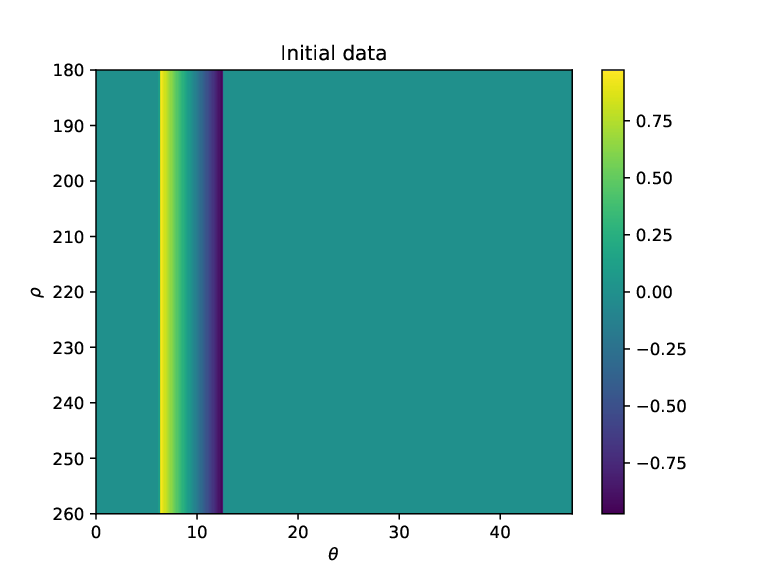
The initial data is chosen as an -wave pulse modeled by:
The absorption parameter will be discussed later in this section. In Fig. 2 we display the initial pulse and the final solution obtained by the five way splitting scheme and the exponential integrator/WENO5 scheme. Here we employ , and for both schemes and display for . The two solutions have a similar shape, but different amplitudes. The difference in amplitude is justified by the employed numerical methods. Indeed, the numerical schemes used in the splitting approach introduce numerical diffusion that is significantly higher than the numerical diffusion introduced by the WENO scheme. Therefore, the amplitude of the solution decreases much faster for the splitting approach than for the new approach presented in section 3.3. The similar shape of the final solutions in Fig. 2 confirms that assuming periodic boundary conditions on rather than homogeneous Neumann boundary conditions does not have appreciable effects on the final solution, at least not in the region of interest: .

| Set 1 | |||
|---|---|---|---|
| Set 2 | |||
| Set 3 | |||
| Set 4 |


4.1 Splitting approach vs. exponential integrator approach
We compare the two approaches by performing numerical simulations for the different values in Table 1. These values are chosen so that the CFL conditions imposed by the splitting approach and the exponential integrator approach are fulfilled. In the splitting approach the CFL conditions imposed by the Godunov and the Lax-Wendroff scheme, used to solve (4), (7), respectively, read
where we used (13) with the estimate . A similar CFL condition applies to the exponential integrator approach. We stress that these conditions are not restrictive, in particular the one imposed on . This allows us to perform numerical simulations choosing reasonable grid sizes.
In Fig. 3 we display the evolution of the numerical solutions obtained by the splitting approach and the exponential integrator approach at different propagation distances along the fixed transverse coordinate . Notice that for the solutions exhibit a -shape profile, similarly to [4]. The profile of the solutions get flatter as increases. This effect is due to the fact that the initial wave travels through the inhomogeneous medium following many different paths. This result in a scattering of the original pulse. Additionally, dissipative effects introduced by the numerical schemes in the splitting approach accentuate the flattening of the original pulse.

Finally, in Table 2 we compare the total time needed to compute the numerical solution at the final propagation for the two approaches and for the different values in Table 1. We observe that the splitting approach is faster for a small number of grid points, but is outperformed by a significant margin (up to a factor of 4 for large resolution) by the ExpRK22 scheme as the grid gets more refined. This is in accordance with the theoretical estimates provided in section 3. Indeed, we have that the splitting scheme requires operations, while the exponential integrator requires operations. In addition, the exponential integrator/WENO scheme introduces less numerical diffusion and avoids oscillations as will be discussed in more detail below.
| Splitting | ExpRK22 | |
|---|---|---|
| Set 1 | s | s |
| Set 2 | s | s |
| Set 3 | s | s |
| Set 4 | s | s |
Absorption parameter. The numerical solutions in the splitting approach are obtained by setting the absorption coefficient . This value is higher than the physical situation would warrant, where we have . The reason of such a choice is to prevent instabilities and/or oscillations of the numerical solutions, see the discussion in [4], section II-A.
We test the new approach presented in section 3.3 for both values of and . In Fig. 4 we compare the numerical solution as a function of obtained by the two methods at . The discretisation is done by employing , and . Notice that oscillations are significantly bigger for the splitting approach, while they are negligible for the exponential integrator approach. The smaller oscillations in the exponential approach are due to use of the WENO scheme. Indeed, WENO schemes are able to capture shocks (i.e. where the solution has less regularity) by reducing the accuracy. However, in smooth regions the scheme recovers its precision, in the specific case the WENO scheme converges with order five. This allows us to choose the coefficient closer to the parameter given by the physical measurements.

Convergence. We test the convergence of the new approach, which is of second order in . To do so, we consider a reference solution obtained by using points in the propagation direction and a final distance . Then, the reference solution is compared with numerical solutions obtained using a smaller number of points in the propagation direction. Both and are computed with the same number of grid points in the coordinate and . In particular, we set and .
We compute the relative error at the final propagation distance read off from
The convergence rate is given by the quotient of two consecutive error values. More specifically, let be two different number of -points for the computation of two numerical solutions and , the associated relative errors. Then, the convergence rate is given by
In Table 3 we collect the relative errors with the convergence rate . Notice that indicates that the employed method is of second order.
| – | ||||||
4.2 High performance computing
We perform numerical simulations by using the exponential integrator method in combination with the WENO5 scheme presented in section 3.3.
For the four different sets of values in Table 1 we measure the total time in seconds needed in order to compute the numerical solution at the final propagation distance . The computer system used is an Intel Xeon scalable CPU Gold 6130 and a Titan V GPU. On the CPU the numerical simulations are performed by using 32 cores.
We carry out four tests. First, we test the sequential code. Second, we parallelize with the application programming interface OpenMP. Third, we parallelize with graphic processing units by using CUDA. In particular, for the GPU implementation we present two versions of the code: one in double precision floating point and one in single precision floating point. Performance results for the four different cases are reported in Table 4. Numerical tests show a drastic speed up achieved using parallelisation with OpenMP compared to the sequential code, which is up to 22 times faster. The simulations are further accelerated when GPUs are involved. In particular, we observe that the single precision floating point implementations on GPUs run more than five times faster than the corresponding CPU implementations. The single precision implementation offers a speed up by a factor roughly two with respect to the double precision implementation, as expected. To trade accuracy for precision might not always be a good choice. However, for this work single precision simulations still offer good results that give insight of the physical phenomena. We stress the fact that performance improvements of the simulations can be obtained only if the algorithm has a high rate of parallelisation. Differently, the simulation times on GPUs might result even inferior to the sequential code.
An interesting aspect in HPC is to compare problems that are compute bound versus problems that are memory bound. Compute bound problems are of the kind that memory access is negligible with respect to the number of arithmetic operations, while the vice-versa holds for memory bound problems. This two aspects find place in the example treated in this work. More specifically the cost of the linear part are essentially memory bound, while the cost of the non-linear part are compute bound. We compare the time required to solve the linear parts against the WENO5 scheme. To illustrate this, let us consider the pseudo-code given in Algorithm 2.
STEP 1 and STEP 3 are responsible for the non-linear effects, while STEP 2 and STEP 4 for the linear ones. In Table 5 we report the required average time to compute the different steps in one iteration. To do so, we measure the total time to the completion of the simulation and divide it by . The results show how the computational cost of the linear effects is lower than the non-linear ones for the sequential simulation. When the code is parallelised the situation is reversed. This is due to the fact that the WENO5 scheme is computationally bound, while the FFT is memory bound.
| Data set | Seq. | OpenMP | CUDA double prec. | CUDA single prec. |
|---|---|---|---|---|
| Set 1 | s | s (x) | s (x) | s (x) |
| Set 2 | .4 s | s (x) | s (x) | s (x) |
| Set 3 | s | s (x) | s (x) | s (x) |
| Set 4 | s | s (x) | s (x) | s (x) |
| Sequential | OpenMP | CUDA double prec. | CUDA single prec. | |
|---|---|---|---|---|
| nonlinear | s | s | s | s |
| linear | s | s | s | s |
5 Conclusions
This work is devoted to the study of the propagation of sonic-booms from the mid field into the far field. The mathematical model is given by a KZK-type equation which is a dispersive nonlinear partial differential equation. In the literature a numerical approach based on splitting methods has been proposed. In this work an adaptation of the algorithm is presented and discussed in details. One of the main disadvantages of the aforementioned approach consists in a difficult parallelisation of the algorithm. Therefore, we present a different approach based on exponential integrators in combination with WENO schemes. The new algorithm is highly parallelisable resulting in a tremendous acceleration (almost up to 185 times faster) with respect to its sequential version. Other than a reduced time of simulations, the exponential integrator approach brings additional benefits. The proposed algorithm achieves an higher accuracy with respect to the splitting approach, moreover the number of operations is (asymptotically) smaller. Finally, we observe numerically a significant reduction of oscillations (in amplitude) of the numerical solutions when the exponential integrator approach is used. The new approach allows us to choose more grid-points and obtain numerical solutions that better describe the physical phenomena of -wave propagation maintaining the time of simulations relatively low.
References
- [1] N. Allahverdi, A. Pozo, and E. Zuazua, Numerical aspects of sonic-boom minimization, in Contemporary Mathematics, vol. 658, American Mathematical Society, Providence, Rhode Island, 2016, pp. 267–279.
- [2] J. J. Alonso and M. R. Colonno, Multidisciplinary optimization with applications to sonic-boom minimization, Annual Review of Fluid Mechanics, 44 (2012), pp. 505–526.
- [3] N. Auer, L. Einkemmer, P. Kandolf, and A. Ostermann, Magnus integrators on multicore CPUs and GPUs, Computer Physics Communications, 228 (2018), pp. 115–122.
- [4] M. Averiyanov, P. Blanc-Benon, R. Cleveland, and V. Khokhlova, Nonlinear and diffraction effects in propagation of N-waves in randomly inhomogeneous moving media, The Journal of the Acoustical Society of America, 129 (2011), pp. 1760–1772.
- [5] M. V. Aver’yanov, V. A. Khokhlova, O. A. Sapozhnikov, P. Blanc-Benon, and R. O. Cleveland, Parabolic equation for nonlinear acoustic wave propagation in inhomogeneous moving media, Acoustical Physics, 52 (2006), pp. 623–632.
- [6] H. Burau, R. Widera, W. Hönig, G. Juckeland, A. Debus, T. Kluge, U. Schramm, T. E. Cowan, R. Sauerbrey, and M. Bussmann, PIConGPU: A fully relativistic particle-in-cell code for a GPU cluster, IEEE Transactions on Plasma Science, 38 (2010), pp. 2831–2839.
- [7] M. Caliari, L. Einkemmer, A. Moriggl, and A. Ostermann, An accurate and time-parallel rational exponential integrator for hyperbolic and oscillatory PDEs. arXiv:2008.11607, 2020.
- [8] N. Crouseilles, L. Einkemmer, and J. Massot, Exponential methods for solving hyperbolic problems with application to collisionless kinetic equations, Journal of Computational Physics, 420 (2020), p. 109688.
- [9] N. Crouseilles, L. Einkemmer, and M. Prugger, An exponential integrator for the drift-kinetic model, Computer Physics Communications, 224 (2018), pp. 144–153.
- [10] L. Einkemmer, Semi-lagrangian Vlasov simulation on GPUs, Computer Physics Communications, 254 (2020), p. 107351.
- [11] L. Einkemmer and A. Ostermann, Exponential integrators on graphic processing units, in 2013 International Conference on High Performance Computing & Simulation (HPCS), IEEE, 2013, pp. 490–496.
- [12] I. Gainullin and M. Sonkin, High-performance parallel solver for 3D time-dependent Schrödinger equation for large-scale nanosystems, Computer Physics Communications, 188 (2015), pp. 68–75.
- [13] M. Griebel and P. Zaspel, A multi-GPU accelerated solver for the three-dimensional two-phase incompressible Navier-Stokes equations, Computer Science - Research and Development, 25 (2010), pp. 65–73.
- [14] M. Hochbruck and A. Ostermann, Exponential Runge–Kutta methods for parabolic problems, Applied Numerical Mathematics, 53 (2005), pp. 323–339.
- [15] M. Hochbruck and A. Ostermann, Exponential integrators, Acta Numerica, 19 (2010), pp. 209–286.
- [16] D. Howe, Improved sonic boom minimization with extendable nose spike, in 43rd AIAA Aerospace Sciences Meeting and Exhibit, Reno, Nevada, 2005, American Institute of Aeronautics and Astronautics.
- [17] G.-S. Jiang and C.-W. Shu, Efficient implementation of weighted ENO schemes, Journal of Computational Physics, 126 (1996), pp. 202–228.
- [18] C. Klein and K. Roidot, Fourth order time-stepping for Kadomtsev–Petviashvili and Davey–Stewartson equations, SIAM Journal on Scientific Computing, 33 (2011), pp. 3333–3356.
- [19] R. J. LeVeque, Numerical methods for conservation laws, Lectures in mathematics, Birkhäuser, ETH Zürich, 1992.
- [20] F. Li, Y. Ye, Z. Tian, and X. Zhang, CPU versus GPU: which can perform matrix computation faster—performance comparison for basic linear algebra subprograms, Neural Computing and Applications, 31 (2019), pp. 4353–4365.
- [21] B. Lipkens, Model experiment to study sonic boom propagation through turbulence. part iii: Validation of sonic boom propagation models, The Journal of the Acoustical Society of America, 111 (2002), pp. 509–519.
- [22] J. Pawlowski, D. Graham, C. Boccadoro, P. Coen, and D. Maglieri, Origins and overview of the shaped sonic boom demonstration program, in 43rd AIAA Aerospace Sciences Meeting and Exhibit, American Institute of Aerounatics and Astrounatics, 2005.
- [23] K. Plotkin, Review of sonic boom theory, in 12th AIAA Aeroacoustic Conference, San Antonio, Texas, 1989, American Institute of Aeronautics and Astronautics.
- [24] R. Seebass and A. R. George, Sonic-boom minimization, The Journal of the Acoustical Society of America, 51 (1972), pp. 686–694.
- [25] J. D. Shanks, W. Liu, and R. Smedley-Stevenson, Revisiting exponential integrator methods for HPC with a mini-application, in 2020 IEEE/ACM 11th Workshop on Latest Advances in Scalable Algorithms for Large-Scale Systems (ScalA), 2020, pp. 19–26.
- [26] C.-W. Shu, Essentially non-oscillatory and weighted essentially non-oscillatory schemes for hyperbolic conservation laws, in Advanced numerical approximation of nonlinear hyperbolic equations, A. Quarteroni, ed., Springer, 1998, pp. 325–432.
- [27] , High order ENO and WENO schemes for computational fluid dynamics, in High-order methods for computational physics, D. H. Barth T.J., ed., Springer, 1999, pp. 439–582.
- [28] M. Wiesenberger, L. Einkemmer, M. Held, A. Gutierrez-Milla, X. Sáez, and R. Iakymchuk, Reproducibility, accuracy and performance of the Feltor code and library on parallel computer architectures, Computer Physics Communications, 238 (2019), pp. 145–156.