The characteristics of cycle-nodes-ratio and its application to network classificationJournal: Journal of LaTeX Templates
Abstract
Cycles, which can be found in many different kinds of networks, make the problems more intractable, especially when dealing with dynamical processes on networks. On the contrary, tree networks in which no cycle exists, are simplifications and usually allow for analyticity. There lacks a quantity, however, to tell the ratio of cycles which determines the extent of network being close to tree networks. Therefore we introduce the term Cycle Nodes Ratio (CNR) to describe the ratio of number of nodes belonging to cycles to the number of total nodes, and provide an algorithm to calculate CNR. CNR is studied in both network models and real networks. The CNR remains unchanged in different sized Erdős-Rényi (ER) networks with the same average degree, and increases with the average degree, which yields a critical turning point. The approximate analytical solutions of CNR in ER networks are given, which fits the simulations well. Furthermore, the difference between CNR and two-core ratio (TCR) is analyzed. The critical phenomenon is explored by analysing the giant component of networks. We compare the CNR in network models and real networks, and find the latter is generally smaller. Combining the coarse-graining method can distinguish the CNR structure of networks with high average degree. The CNR is also applied to four different kinds of transportation networks and fungal networks, which give rise to different zones of effect. It is interesting to see that CNR is very useful in network recognition of machine learning.
Keywords:
Cycle nodes ratio , Network classification, Giant component , Depth first search1 Introduction
The study of network structures is a key point in the initial stage of network science. The cycle property as the basic property of graph has been studied extensively [1]. The cycles play crucial roles in network spreading [2, 3], community detection [3], and network control [4], etc. Bianconi et al [5] studied the statistic of cycles in Barabási-Albert (BA) [6] scale-free networks and obtained: , where , represents the number of loops with length , represents the number of added edges at every step in BA model, and is size of network. Noh [7] calculated the distributions of cycles in both uncorrelated networks and correlated ones. At nearly the same time the study of the tree property in complex networks began to prevail. Gu et al [8] incorporated small-world effect and scale-free property into a tree-like network model. Wechsatol et al [9] found the cycles can enhance the robustness of the network. And it was paid attention again recently to study the effects of cycles [10, 11, 12, 13, 14]. Wylie et al [10] found the switch integration in biological networks is controlled by the cycles but not the network hubs. Fan et al [11] studied the properties of loops in network models, based on which the node’s importance can be quantified. Given the proportion of minimum feedback vertex set, Zhou et al [15, 12] proposed an algorithm to search for the minimum number of feedback edges, and they concluded the feedback vertices are important for the structural and dynamical properties of directed networks. Shi et al [13] proposed to search for linearly independent cycles of a network, which was used in studying the cyclic structures in small-world networks. Wu et al [14] discussed the bridges in complex networks, and proposed the concept of bridgeness to represent edge centrality. Lately, there has been great interest in network classification by using the method of machine learning. Kantarc et al [16] classified the networks by the topological quantities. They considered 14 different topological measures to characterize the networks, and found that the most favorable measures are density, modularity, average degree, and transitivity (global clustering coefficient). Niousha et al [17] also proposed the method of network classification based on the supervised learning and distance-based classification algorithm, which has high classification accuracy, noise tolerance, and computation efficiency.
Although the structure of cycles is important and some qualities can describe the richness of cycles. But there is no more intuitive quality, to our best knowledge, to tell whether a given network tends to be tree-like or not. We have studied the cycle properties in Ref. [18], and found that it is crucial for transportation whether the ports are located along with cycles or not in world marine networks. Here we introduce the Cycle Nodes Ratio (CNR) of a given network, defined as the ratio of nodes belonging to cycles to the number of total nodes. The algorithm of calculating the number of cycles is hard in networks. Here we propose an algorithm, named CDFS, based on the Depth First Search (DFS) [19] algorithm, to calculate the CNR for the network of interest. The LDFS has low computation complexity , where and are the numbers of nodes and edges, respectively. We calculate the CNR of three basic random networks and identify critical transition points in Erdős-Rényi (ER) [20] networks, as well as the underlying mechanism. The approximate analytical solution of the CNR in ER networks is given by calculating the giant component in ER networks. Otherwise, the CNR is 1 in both BA networks and Watts-Strogatz (WS) networks [21] with average degree no less than 4. In this process, we proved the key difference between CNR and two-core ratio (TCR) in WS network and fungal growth network. We also calculate the CNR in real networks by using different data sets, which are slightly lower than the counterparts of ER networks with the same average degree. To judge the CNR properties of networks in which the smallest degree is greater than 1, we combine the improved spectral coarse-graining (ISCG) [22] to test the CNR of the macroscopic property of this kind of networks. Last but not least, we compare the CNR in different kinds of networks, and consider the CNR, density, modularity [23], average degree, and global clustering coefficient [24], as the features to be classified by K-Nearest Neighbor (KNN) algorithm [25]. We have found that CNR is the most important feature for network classification.
The rest of this paper is organized as follows: the concept of CNR and the corresponding algorithm are given in Sec. 2. Sec. 3 discusses the CNR properties in random networks and the approximate analytical solution of CNR in ER networks. The CNR is studied for different kinds of complex networks in Sec. 4, as well as its significance in classification of networks by machine learning. The last section contains the conclusion including the applications and the improvement of CNR.
2 The definition of cycle nodes ratio and its algorithm
2.1 Cycle nodes ratio
As we know, the cycle in a network is defined as: a cycle is an elementary chain which returns to the initial node [26], as shown in Fig. 1. And we introduce the definition of the cycle nodes as:
Cycle node: the node sites along one or more cycle(s) path in a network.
An example of a cycle nodes is shown in Fig. 2. The concept of cycle node is different from the concept of k-core, which is defined as the remaining nodes by recursively deleting the leaf nodes [27], We refer to nodes similar to node 7 as cycle connect node which is not cycle node but can connect different cycles. The proportion of cycle nodes in a network can represent the characteristics of how far a network is away from tree networks in which no cycle exists. The CNR can be defined as:
Cycle nodes ratio: Suppose for an undirected, connected graph with vertices and edges, the number of cycle nodes is . The cycle nodes ratio is , where is the number of nodes in .
The CNR is 1 in cycle graph and 0 in tree (star) graph as shown in Fig. 3. Clearly, the normalization is satisfied.
2.2 The algorithm of calculating CNR
The statistics of the cycles in complex networks is a hard job [5]. It is almost impossible to judge whether a node is cycle node by calculating the number of cycles in a given network. But we find that a node is cycle node if there is no-cut edge connecting to it. The cut edge is defined in graph theory [28] as:
Cut edges: In a graph, if removing a given edge causes the addition of one connected component of this graph, then this edge is called cut edge, which also known as bridge (Shown in Fig. 2).
The edge is simply called no-cut edge if it is not cut edge, and the cut edges can be recognized by Tarjan algorithm [19]. We here introduce some basic concepts of Tarjan algorithm:
- 1.
Depth First Search (DFS) search tree: We can get the DFS search tree from graph ergodic by DFS, shown in Fig. 4(b).
- 2.
Tree edges: In the DFS process, the passing edges of visiting the nodes which are not visited, like the edges not labeled in Fig. 4(b).
- 3.
Back edges: In the DFS process, the passing edges of visiting the nodes which are visited, like the edges labeled in Fig. 4(b).

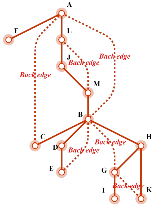
For a node , we need to record two values that are which represents the order of node in the DFS process, and which represents the node that can retrospect the earliest node and not pass through its father node. The and are added 1 in the each step of DFS process, then we recalculate the from the root node by following the rule that
The edge is cut edge if . The DFS result of Fig. 4(a) is shown in Table. 1, the top line represents the node, and the second line and third line represent the and of the corresponding node respectively. Otherwise, the DFS just traverses the nodes which are in the same component as father node of this algorithm. So we can take one chosen node of each component as the father node of DFS for networks with multi-components. This algorithm is shown in Ref. [29]. Then we can get the corresponding cut edges. For a graph with vertices and edges, the time complexity of this algorithm is for adjacency list data or for adjacency matrix data. This algorithm has high efficiency in classifying cycle nodes and non-cycle nodes in a network.
| Node | A | B | C | D | E | F | G | H | I | J | K | L | M |
|---|---|---|---|---|---|---|---|---|---|---|---|---|---|
| 1 | 5 | 12 | 11 | 10 | 13 | 8 | 6 | 9 | 4 | 7 | 2 | 3 | |
| 1 | 1 | 1 | 5 | 5 | 13 | 5 | 5 | 9 | 2 | 5 | 1 | 1 |
3 The simulation and analytical results of CNR in networks
3.1 The simulation results of CNR and its applications in basic random networks
To study the properties of CNR, we calculate its value in ER networks. In the first approach, we fix the average degree and change the size of networks, and in the second one, we fix the size of networks and change the average degree. The results are shown in Fig. 5. The major findings are concluded as follows:
- 1.
The CNR of ER model remains constant in different sized networks if the average degree of ER networks is fixed.
- 2.
If we fix the size of ER networks, the value of CNR will increase with the average degree of ER networks.
- 3.
A critical turning point occurs when the average degree of ER networks is 1.
The simulation results of WS networks are shown in Fig. 6. Firstly, the average degree is fixed at 2, and we study the change of CNR with network size at rewiring probabilities of 0.1 and 0.2, respectively. Since the WS networks are generated from regular networks (with mean degree of 2), their CNR have higher uncertainty in the rewiring process. The CNR will stabilize with increased network size. And the CNR is 0.45 if the average degree is 2 and 1 if the average degree is greater than 4 with low rewiring probability. But they show different tendencies when the rewiring probability is increased. The CNR of WS networks with average degree 4 will decrease with the rewiring probability and the CNR of WS networks with average degree 2 will increase slowly with rewiring probability. This is due to the fact that WS networks with high rewiring probability tend to be like ER networks. It is then not strange that the CNR’s of the two are close to one another.
In the modeling of BA networks, if exactly one edge and one node are added at every step, the CNR will be 0 in this network, since this network is a tree network. Otherwise, the CNR will be 1 if more edges than one are added since every node constitutes a cycle when added.
To compare the difference between cycle node and two-core node, we study the CNR and two-core-ratio (TCR) in both ER networks and WS networks. CNR and TCR are very similar in ER networks, but much different in WS networks (shown in Fig. 7). As shown in Fig. 2, cycle connect nodes (node 7) is the key factor that leads to the difference in cycle node and two-core node. In WS networks, cycle connect nodes are easy to generate as WS networks have a single line (the line constituted by nodes and edges one by one), the nodes contained in this kind of structure are often seen as two-core nodes but unlikely to be cycle nodes. For example, Fig. 8(a) shows the difference between cycle nodes and two-core nodes. This cycle connect nodes appears frequently in fungal growth networks (shown in Fig. 8(b)).
The node centrality is introduced to describe the importance of nodes in complex networks. The commonly used centrality measures are degree centrality, betweenness centrality [30], PageRank centrality [31], closeness centrality [32], etc. We have defined the cycle centrality of node i as the number of nodes which are transformed from cycle nodes to none-cycle nodes with node i being deleted. For example, in the below Fig. 9, node 22 has the largest cycle centrality, that is 16, in this network, and its deletion will transform cycle nodes to none-cycle nodes. Therefore, cycle centrality can represent the over-distance connection capability of the node. Because if you delete this node, the shortest-path lengths of its neighboring nodes will greatly increase. The node which has large cycle centrality can decrease the average shortest-path length of network.
3.2 The analytical result of CNR in ER networks
In this part, the analytical solution of CNR in ER networks is given. Generally speaking, one node could be a cycle node if it is connected to two nodes that belong to one component in a network (The two nodes could contact through this network, as shown in Fig. 10). Suppose there are components in ER-network , and is the number of nodes in component . The number of all contact pairs is
| (1) |
Then the probability that nodes with degree 2 are cycle nodes is
| (2) |
where is the nodes number of the ER network. Otherwise the probability of finding the node with degree in ER networks is [33]:
| (3) |
where is the connecting probability of different nodes in ER-networks. And the probability of nodes, with different degrees, being a cycle node in ER networks is shown in Tab. 2. The summation of the probabilities over all nodes in ER-networks gives the CNR
| (4) |
Then we have the simulation of CNR in ER networks by Eq. 4 which is shown in Fig. 11. The CNR calculated by the network components is fairly consistent with the simulation result.
| 2 | |
|---|---|
| 3 | |
| 4 | |
| ⋮ | ⋮ |
Consider the ER-network with size and connecting probability , the number of nodes on tree components of () is (see in Red. [34])
| (5) | |||||
where is the number of components in that are trees of size , and is the average degree of . is the probability of a node belonging to the tree component. By the manipulations of Eq. 5, is the only solution of
| (6) |
in the range . So
| (7) |
This result means that all nodes on the tree components, and the number of nodes on cycles is 0 for . In the range , is the union of the giant component , the small unicyclic components and the small tree components. There are at most vertices on the unicyclic components [34]. The size of the giant component satisfies (see in Ref. [34])
| (8) |
From Ref. [34] we get
| (9) |
and since
| (10) | |||||
for every , since for . Thus , and
| (11) |
Then we conclude that (according to [20, 35])
| (12) |
This result is shown in Fig. 12, which is consistent with the simulation result. By Eq. 2, can be calculated as:
| (13) | |||||
where Eq. 11 is used, and the third term could be omitted if . Combining Eqs. 3, 4, 13 and , the CNR could be written as:
| (14) | |||||
Since decays rapidly with , so we calculate it for , which is shown in Fig. 13. The analytical result is in accordance with the simulation result. And the giant component, which appears when , leads to the turning point of CNR. The analytical result is close to the analytical result of TCR which has been observed in Ref. [36]. These two analytical results have different analytic forms which are caused by different methods, even though they have very similar results in ER networks. Besides, our method is easier to understand and calculate.
4 The CNR in real networks and its application in network classification
4.1 CNR in real networks, and used in conjunction with improved spectral coarse-graining
To study the properties of CNR in real networks, we employ the data samples from network repository [37], Stanford Large Network Dataset [38], Pajek datasets [39], and some classic complex networks [40, 41, 42, 43, 44, 45, 46]. unweighted and undirected complex networks were chosen randomly. The size of these networks is between and , and their edges range from to .
Their CNR and average are calculated and compared with ER network, as shown in Fig. 14. The CNR of real networks increases with the increase of average degree, and has a similar trend with that of the ER networks. But it is obvious that the CNR of real networks is lower than that of the ER networks and much lower than that of the BA networks and WS networks (the value of CNR is in BA and WS networks when the degree is large than 4). So, we argue that the networks generated by basic network models cannot produce the exact CNR properties. The real networks are much more tree-like compared with the network models.
In real networks, we find that most networks with high average degree have CNR close to 1. But their macroscopic properties do not look like cycles if we zoom out the networks. So if we want to measure the CNR of macro states of these graphs, we should combine the improved spectral coarse-graining (ISCG) [22]. The ISCG is a new method to coarse-grain the graph based on the spectral coarse-graining (SCG) [47]. Compared to the SCG method, the ISCG algorithm has many advantages such as smaller errors, better effects, and greatly reduced computational complexity. For the two networks in Fig. 15, both of their CNR are 1, but it is obvious that the right one is more like cycle and the left one is more close to a line. Coarse-graining these two networks by ISCG, we got the corresponding new networks under them (the number of nodes is reduced by two-thirds). The new CNR of these two networks is 1 and 0.1875, respectively. In the transport and flow networks, the macro-structure is important than the micro-structure. In this case, calculation of the CNR of the coarse-graining networks is useful and feasible.
4.2 The application of CNR in network classification
Then we study the transport networks, and find that different kinds of transport networks tend to form different zones which barely overlap with each other (shown in Fig. 16). That is to say, they can be classified by different zones. To be more compelling, we also included the network set of public transportation in different cities and fungal growth network for classification. The datasets for classification contain 28 subway networks of different cities, 41 marine transport networks of different companies, 21 airline networks of different companies, 405 cities’ public transportation networks of different cities in China, and 270 fungal growth networks. All these datasets can be downloaded from Ref. [29]. The basic properties of these networks are shown in Table. 3.
| Network | ||||
|---|---|---|---|---|
| Subway networks | 68595 | 69741 | 2.0152.491 | 00.0319 |
| Marine transport networks | 12356 | 17844 | 2.5126.056 | 0.1090.519 |
| Airline networks | 17123 | 16521 | 1.8828.472 | 0.08030.493 |
| Fungal growth networks | 692741 | 723665 | 1.6073.254 | 0.005950.207 |
| Public transportation networks | 813133 | 819905 | 24.620 | 00.152 |
These five datasets are classified by employing the machine learning metric of K-Nearest Neighbor (KNN) algorithm [25]. The basic process of the algorithm is to calculate the distance in characteristic space and identify the category of most samples of the nearest neighbor of the new sample belongs to, then set the new sample belonging to this category. As the results of Ref. [16], we choose the four most discriminant features and CNR to be the machine learning parameters: the density , modularity , average degree , global clustering coefficient , and CNR. The density is the ratio of existing edges to the number of all possible edges in network .
| (15) |
The modularity is the quantity which shows the quality of the community structure. It is the proportion of links inside the communities minus the estimated result from the corresponding null model. The global clustering coefficient refers to the proportion of triangles, which measures the connection density among neighboring nodes of one node.
We classify this network set in six different approaches. In the first one, all five features are chosen, and four features out of five are chosen in the next five approaches. The classification result is shown in Tab. 4, and the accuracy of classification without the CNR is significantly lower than the rest ones with the CNR. This means that the CNR can increase the accuracy of network recognition in machine learning obviously. So we think the CNR is one important property of networks, which can not only show whether the networks tend to be tree-like or cycle-like, but can distinguish different kinds of networks.
| Features | Precision | Recall | F1-score | Support |
|---|---|---|---|---|
| All five features | 0.91 | 0.92 | 0.91 | 192 |
| Without | 0.90 | 0.91 | 0.90 | 192 |
| Without | 0.89 | 0.90 | 0.89 | 192 |
| Without | 0.89 | 0.90 | 0.89 | 192 |
| Without | 0.91 | 0.92 | 0.91 | 192 |
| Without | 0.80 | 0.80 | 0.79 | 192 |
5 Conclusions
In this paper, we have proposed the concept of CNR to judge whether the network tends to be treelike or not, and an algorithm to calculate this quantity. The CNR is constant with different sized networks, and displays critical turning points in ER networks. TCR is greater than CNR in WS networks and some real networks. The cycle centrality is introduced to describe over-distance connection capability of the node among its neighboring nodes. We have provided the analytical solution of CNR in ER networks, which can explain the critical turning in ER networks by giant component. We then study the CNR in real networks, and find that its value is lower than that of the basic networks models with the same average degree. In addition, it is useful to combine the coarse-graining method to judge the cycle structure of networks. Finally, we have classified the networks of different kinds by machine learning. The CNR is found to be the most compelling feature to enhance the accuracy of classification. Therefore we may regard the CNR as one essential quantity of complex networks.
Acknowledgements
We gratefully acknowledge Linyuan Lü, Haijun Zhou, Liping Chi, and Shengfeng Deng, give us fruitful suggestions. Thanks to Yueying Zhu, Longfeng Zhao, and Jiao Gu for offer help on network data. This work was supported in part by National Natural Science Foundation of China (Grant No. 61873104, 11505071), the Programme of Introducing Talents of Discipline to Universities under Grant No. B08033, the Fundamental Research Funds for the Central Universities.
References
- [1] F. Solimano, E. Beretta, Graph theoretical criteria for stability and boundedness of predator-prey systems, Bulletin of Mathematical Biology 44 (4) (1982) 579–585.
- [2] G. T. Cantwell, M. E. J. Newman, Message passing on networks with loops, PNAS 116 (47) (2019) 23398–23403.
- [3] V. Kuikka, Influence spreading on complex networks–effects of node activity and paths with loops, International Journal Of Engineering Research And Development 14 (02).
- [4] J. C. Rozum, R. Albert, Identifying (un) controllable dynamical behavior in complex networks, PLoS computational biology 14 (12) (2018) e1006630.
- [5] G. Bianconi, A. Capocci, Number of loops of size in growing scale-free networks, Physical Review Letters 90 (7) (2003) 078701.
- [6] A.-L. Barabási, R. Albert, Emergence of scaling in random networks, Science 286 (5439) (1999) 509–512.
- [7] J. D. Noh, Loop statistics in complex networks, European Physical Journal B 66 (2) (2008) 251–257.
- [8] Y. Gu, J. Sun, A tree-like complex network model, Physica A: Statistical Mechanics & Its Applications 389 (1) (2010) 171–178.
- [9] W. Wechsatol, S. Lorente, A. Bejan, Tree-shaped networks with loops, International Journal of Heat and Mass Transfer 48 (2005) 573–583. doi:10.1016/j.ijheatmasstransfer.2004.08.020.
- [10] D. C. Wylie, Linked by loops: Network structure and switch integration in complex dynamical systems, Physica A: Statistical Mechanics & Its Applications 388 (9) (2012) 1946–1958.
- [11] T. Fan, L. Lü, D. Shi, Towards the cycle structures in complex network: A new perspective, arXiv preprint arXiv:1903.01397.
- [12] Y. Z. Xu, H. J. Zhou, Optimal segmentation of directed graph and the minimum number of feedback arcs, Journal of Statistical Physics 169 (1) (2017) 187–202.
- [13] D. Shi, L. Lü, G. Chen, Totally homogeneous networks, National Science Review 6 (5) (2019) 962–969.
- [14] A.-K. Wu, L. Tian, Y.-Y. Liu, Bridges in complex networks, Physical Review E 97 (1) (2018) 012307.
- [15] H.-J. Zhou, Spin glass approach to the feedback vertex set problem, The European Physical Journal B 86 (11) (2013) 455.
- [16] B. Kantarci, V. Labatut, Classification of complex networks based on topological properties, in: 2013 international conference on Cloud and Green Computing, IEEE, 2013, pp. 297–304.
- [17] N. Attar, S. Aliakbary, Classification of complex networks based on similarity of topological network features, Chaos: An Interdisciplinary Journal of Nonlinear Science 27 (9) (2017) 091102.
- [18] W. Zhang, W. Deng, W. Li, Statistical properties of links of network: A survey on the shipping lines of worldwide marine transport network, Physica A: Statistical Mechanics and its Applications 502 (2018) 218–227.
- [19] R. Tarjan, Depth-first search and linear graph algorithms, SIAM journal on computing 1 (2) (1972) 146–160.
- [20] P. Erdős, A. Rényi, On the evolution of random graphs, Publ. Math. Inst. Hung. Acad. Sci 5 (1) (1960) 17–60.
- [21] D. J. Watts, S. H. Strogatz, Collective dynamics of ‘small-world’networks, Nature 393 (6684) (1998) 440.
- [22] J. Zhou, Z. Jia, K.-Z. Li, Improved algorithm of spectral coarse graining method of complex network, Acta Physica Sinica 66 (6) (2017) 060502.
- [23] M. E. J. Newman, Fast algorithm for detecting community structure in networks, Physical Review E 69 (6) (2004) 066133.
- [24] S. Wasserman, K. Faust, et al., Social network analysis: Methods and applications, Vol. 8, Cambridge university press, 1994.
- [25] J. M. Keller, M. R. Gray, J. A. Givens, A fuzzy k-nearest neighbor algorithm, IEEE transactions on systems, man, and cybernetics (4) (1985) 580–585.
- [26] C. A. Holzmann, F. Harary, On the tree graph of a matroid, SIAM Journal on Applied Mathematics 22 (2) (1972) 187–193.
- [27] B. Pittel, J. Spencer, N. Wormald, Sudden emergence of a giantk-core in a random graph, Journal of Combinatorial Theory, Series B 67 (1) (1996) 111–151.
- [28] H. Fleischner, Eulerian graphs and related topics, Vol. 1, Elsevier, 1990.
- [29] W. Zhang, Lno algorithm and dataset, https://github.com/wenjun314/Loop-node-occupation.
- [30] L. C. Freeman, A set of measures of centrality based on betweenness, Sociometry (1977) 35–41.
- [31] Google, Facts about google and competition.
- [32] A. Bavelas, Communication patterns in task-oriented groups, The journal of the acoustical society of America 22 (6) (1950) 725–730.
- [33] M. E. J. Newman, S. H. Strogatz, D. J. Watts, Random graphs with arbitrary degree distributions and their applications, Physical Review E 64 (2) (2001) 026118.
- [34] B. Bollobás, B. Béla, Random graphs, no. 73, Cambridge university press, 2001.
- [35] P. Erdős, A. Rényi, On the strength of connectedness of a random graph, Acta Mathematica Hungarica 12 (1-2) (1961) 261–267.
- [36] J.-H. Zhao, H.-J. Zhou, Y.-Y. Liu, Inducing effect on the percolation transition in complex networks, Nature Communications 4 (2013) 2412.
- [37]
R. A. Rossi, N. K. Ahmed, The network data
repository with interactive graph analytics and visualization, in: AAAI,
2015.
URL http://networkrepository.com - [38] J. Leskovec, A. Krevl, SNAP Datasets: Stanford large network dataset collection, http://snap.stanford.edu/data (Jun.).
- [39] V. Batagelj, A. Mrvar, Pajek datasets [ol], hup://vladojmJuni-lj. si/pub/networks/data.
- [40] E. Kolaczyk, Analysis of network data: Methods and models (2009).
- [41] Newman, M. E. J., The structure of scientific collaboration networks, Proceedings of the national academy of sciences 98 (2) (2001) 404–409.
- [42] Newman, M. E. J., Scientific collaboration networks. i. network construction and fundamental results, Physical review E 64 (1) (2001) 016131.
- [43] S. Gopal, The evolving social geography of blogs 88 (1) (2007) 275–293.
- [44] D. Lusseau, The emergent properties of a dolphin social network, Proceedings of the Royal Society of London. Series B: Biological Sciences 270 (suppl_2) (2003) S186–S188.
- [45] M. Girvan, M. E. J. Newman, Community structure in social and biological networks, Proceedings of the national academy of sciences 99 (12) (2002) 7821–7826.
- [46] W. W. Zachary, An information flow model for conflict and fission in small groups, Journal of anthropological research 33 (4) (1977) 452–473.
- [47] D. Gfeller, P. De Los Rios, Spectral coarse graining of complex networks, Physical review letters 99 (3) (2007) 038701.