HVAC Scheduling under Data Uncertainties: A Distributionally Robust Approach

In SP, the probability distributions of stochastic variables are used to generate scenarios, and an optimal solution is found across all scenarios. There are variations in SP formulations, yet the scenario-based approach is straightforward and useful [18].

In our application, each scenario is a one-day temperature profile. The objective function of SP is to minimize the weighted average energy cost of all scenarios as formulated in (2) where subscription $h$ denotes the scenario index and $H$ is the total number of scenarios.

Two types of temperature constraint formulations could be incorporated. A conservative one is formulated in (3), where the indoor air temperature of all scenarios and all steps are strictly limited within the comfort zone, referred to as SP-strict in this paper. The less conservative way is formulated in (4), where temperature violation under individual scenario is allowed, but the expected indoor air temperature overall scenarios have to satisfy the comfort zone limit. It is referred to as SP-average in this paper.

The minimum up and down time constraints of SP are similar to DO’s in (1), except for their dimension being expanded to all scenarios.

SP method aims to solve the robustness issue but suffers from the complexity issue. To achieve a high confidence level of feasibility and optimality, the number of scenarios required is usually large and the computational complexity of SP increases with the scenario set size. To improve the computational efficiency, the RO formulation can be used to optimize the HVAC schedule under the worst scenario of day-ahead ambient temperature within an uncertainty set. Now the objective function is modified to (5), indicating a two-stage formulation. The first stage is still to minimize the total energy cost, and the second stage is to find the worst case scenario, where the power consumption reaches maximum under the worst ambient temperature $T_{t}^{oa*}$. Note that $P_{t}$ is a linear function of $T^{oa}_{t}$ and the first-stage decision variable $x$ is considered as a constant in the second stage, the decision variable of the second-stage problem is the ambient temperature $T^{oa}_{t}$.

Note that in our paper, $\phi$ is the interval uncertainty set that varies with the predicted outdoor air temperature, i.e., $\phi_{t}=[\bar{\phi}_{t},\underline{\phi}_{t}]$.

Without loss of generality, the robust counterpart (RC) of (5) can be reformulated to a tractable linear programming (LP) (24) in Appendix A.

The SP formulation explicitly considers the uncertainty, but scalability becomes a challenge due to the number of scenarios required. In contrast, the RO formulation provides a fast and robust solution but it tends to be too conservative in practice. To overcome the shortcomings, we look at the uncertainty of entire probability distribution rather than a single prediction point using Distributionally Robust Optimization (DRO).

The proposed DRO formulation is presented below.

The initial formulation of DRO given in (6) is a two-stage problem, where the first-stage minimizes the total energy cost. The deterministic constraints (1b)-(1g), and (1j)-(1k) are implemented in the first-stage problem. The challenge lies in the second stage given by (6b), where the expected indoor air temperature under the worst probability distribution needs to be bounded within the comfort range. $\mathcal{P}_{t}$ is a Wasserstein ball (WB) ambiguity set defined in (6c), where $\mathbb{P}_{t}$ denotes an element distribution that has a Wasserstein distance to the center probability distribution $\mathbb{Q}_{t}$ within a radius $\varepsilon$. $W(\cdot)$ is the function of Wasserstein distance formulated in (7) [19].

Let $\tilde{\xi}_{i}$ and $\tilde{\xi}_{j}$ denote the $i^{th}$ and $j^{th}$ discretized value of $\mathbb{Q}$ and $\mathbb{P}$ and $q_{i}$ and $p_{j}$ are their probabilities respectively. Let $\pi\in\mathcal{R}^{I\times J}$ be the joint distribution matrix of the two distributions. The Wasserstein metric is the minimum effort needed to transform one distribution into the other. Note that the two probability distributions have an equal area of 1, and the difference lies in their shapes. Fig. 1 further illustrates the relationship, where the column-wise summation of $\pi$ is the probability distribution of $\mathbb{P}$, and the row-wise summation is the probability distribution of $\mathbb{Q}$. The sum of the entire $\pi$ matrix equals 1. Since $\pi$ is not unique, Wasserstein metric is to find an optimal $\pi$ that minimizes the cost of transformation.

In our case, the center distribution $\mathbb{Q}$ is the predicted empirical distribution and the radius $\varepsilon$ determines the conservativeness of the ambiguity set. Every probability distribution within the WB is a candidate and there are infinitely many of them as long as $\varepsilon>0$. When $\varepsilon=0$, the DRO problem becomes an SP problem, otherwise the DRO problem under its initial formulation is intractable.

To further illustrate the WB ambiguity set, let’s consider an example where the empirical distribution $\mathbb{Q}_{1}$ is given in (8). $\mathbb{Q}_{1}$ is essentially a value prediction in the form of a probabilistic prediction. The probability of the predicted value $75$ is 100%.

Now, consider $74^{\circ}F$ and $78^{\circ}F$ as two possible temperature values in the candidate distribution $\mathbb{P}$. Given a Wasserstein distance $\varepsilon=2$, the worst probability distribution can be solved intuitively. Clearly, $78^{\circ}F$ is the value that results in a higher room temperature, therefore the higher the $p_{(78^{\circ}F)}$ is, the worse the distribution is. The global worst distribution would be $p^{\dagger}_{(78^{\circ}F)}=100\%$ and $p^{\dagger}_{(74^{\circ}F)}=0\%$. The Wasserstein distance between $\mathbb{P}^{\dagger}$ and $\mathbb{Q}_{1}$ is $(78-75)\times 100\%=3$. Such a $\mathbb{P}^{\dagger}$ is infeasible because it is outside of the ambiguity set. Therefore, we decrease the probability of $78^{\circ}F$, and move $\mathbb{P}$ closer to the ambiguity set. It can be concluded that the feasible worst distribution $\mathbb{P}^{*}$ must be sitting on the WB surface, where (9) holds.

Considering $p^{*}_{(74^{\circ}F)}=1-p^{*}_{(78^{\circ}F)}$, we can solve for the worst probability distribution as $p^{*}_{(78^{\circ}F)}=50\%$ and $p^{*}_{(74_{\circ}F)}=50\%$. A generalized solution considering two discretized values in $\mathbb{P}$ is derived in Appendix B.

Incorporating (6c) into (6b), the definition of WB becomes a constraint of second-stage problem, which is given by the left-hand-side (LHS) of (10).

Substituting the room temperature $T_{t}^{in}$ in (10) with the ARX model (1j), the expression of $\mathbb{E}_{\mathbb{P}_{t}}\left[T^{in}_{t}\right]$ becomes (11a), where $\tilde{T}_{j,t}$ denotes the $j$th discretized value with probability $p_{j,t}$. $\tilde{T}^{in}_{j,t}$ and $\tilde{T}^{oa}_{j,t}$ are discretized values of indoor temperature and ambient air temperature probability distributions.

Incorporating (7) and (11) into (10), we obtain (12). Note the inner minimization problem is in the ”$Inf\leq$” format, meaning if there exists a $\pi_{ij,t}$ that meets the condition, the constraint satisfies. Therefore, minimization can be removed and expression (12) can be simplified to regular constraints in (13) [19].

By now, the proposed second-stage DRO constraint (6b) is transformed into the linear constraint in (13), where the goal is to find the worst probability distribution $\mathbb{P}_{t}$ that is bounded within the WB of the empirical probability distribution $\mathbb{Q}_{t}$. $T_{t-1}^{in}$ and $x_{t}$ are not second-stage decision variables, therefore can be regarded as constants.

The LHS of (13) can be further reformulated into (14) by substituting $p_{j,t}$ in the objective function with $\sum_{i=1}^{I}\pi_{ij,t}$ to cancel out $p_{j,t}$. Then $\pi_{ij,t}$ becomes the only decision variable of the second-stage problem.

Let $\lambda_{t}$ and $s_{i,t}$ be the Lagrangian multipliers, the Lagrangian function of (14) is the $\mathcal{L}_{t}\left(\pi_{t},\lambda_{t},s_{t}\right)$ formulated in (15), which can be further reformulated into (16) by aggregating the $\pi_{ij,t}$ terms.

Considering $\pi_{ij,t}\geq 0$, there exists a bounded supremum only if the coefficient of $\pi_{ij,t}$ is non-positive, i.e. $\left|\tilde{T}^{oa}_{i,t}-\tilde{T}^{oa}_{j,t}\right|\lambda_{t}+s_{i,t}\geq b_{2}\tilde{T}^{oa}_{j,t}$. The supremum $p^{*}=\varepsilon\lambda_{t}+\sum_{i=1}^{I}q_{i,t}s_{i,t}+\left(b_{3}T^{in}_{t-1}+b_{1}x_{t}+b_{0}\right)$ is achieved at $\pi_{ij,t}=0$. According to the strong duality theorem [20], the Lagrangian function becomes a function of $\lambda_{t}$ and $s_{i,t}$, and its infimum is equal to the supremum of the original problem. Hence, the maximization problem in (14) is dualized into a minimization problem (17). Together with the upper bound of the temperature setpoint, constraint (13) becomes the inequality (17).

Similar to the sub-problem in (12), the ”min” can be removed due to ”$Inf\leq$” format. Hence, the final tractable formulation of the proposed DRO under cooling conditions is given by (18).

This subsection aims to provide a straightforward test case following the example in Section IV-A with $\mathbb{Q}_{1}$ being the ambient temperature forecast of $75^{\circ}F$. The example given is a single-step decision-making considering two possible ambient temperature values. The power consumption model and room temperature model incorporated in this case are formulated in (19). The room temperature at the previous step is $T^{in}_{0}=76$, and the upper bound of comfort zone is set to $76^{\circ}F$. Then the initial formulation of this case can be formulated as (20), where the $WB(\mathbb{Q}_{1},2)$ denotes the Wasserstein ball with the center of $\mathbb{Q}_{1}$ and a radius of $\varepsilon=2$.

The results of 7 scenarios with prediction of $\mathbb{Q}_{1}$ are summarized in Table I, where $\mathbb{E}\left[T^{in}\mid_{x=1}\right]$ and $\mathbb{E}\left[T^{in}\mid_{x=0}\right]$ are the expected value of room temperature with and without HVAC under the worst case distribution which is shown in columns 2 and 3. $x^{*}$ is the optimal HVAC on/off status solved by the tractable formulation of the proposed DRO method. Take the first case for example. When two discretized value $75^{\circ}F$ and $77^{\circ}F$ are considered, the worst probability distribution is when $p_{77^{\circ}F}=1$. Inserting this probability into (20b), we find that the expected indoor temperature is $76.3^{\circ}F$ when HVAC is off and $73.3^{\circ}F$ when HVAC is on. To avoid temperature violation, HVAC needs to be on $(x=1)$, which is exactly the solution from tractable reformulation (18). The solutions from all seven cases can be manually computed to confirm the correctness of tractable reformulation (18) from the very original two-stage DRO formulation (6). It is also noted that different discretization values impact the optimal solutions.

The practical test case utilizes real measurement data collected from a commercial building to learn the zone temperature and power consumption model. Table II summarizes the coefficients of the models used in this case.

The DO, SP, RO, and the proposed DRO methods are implemented to solve the one-day schedule of the building. The obtained optimal schedules are tested under two testing sets, the regular scenario testing set and the extreme scenario testing set, to validate their optimality and robustness. Each testing set contains 1000 randomly generated scenarios. The scenarios in the regular testing set are sampled from the predicted Gaussian distribution, while the scenarios in the extreme testing set are sampled from a set of distributions randomly, including Gaussian distribution with inaccurate mean and standard deviation, uniform distribution with random ranges, and beta distribution with random parameters of $\alpha$ and $\beta$, to mimic the unknown nature of underlying probability distributions of ambient temperature.

The optimality evaluation metric is the total cost. The robustness evaluation metrics are the number of steps with temperature violations $\left(V^{num}\right)$, and the temperature violation mileage $\left(V^{mil}\right)$, defined in (21), where $\mathbbm{1}(\cdot)$ is the indicator function.

The predicted outdoor air temperature is assumed to follow Gaussian distributed in the day-ahead prediction, and the predicted mean value $\mu_{t}$ over the day is indicated by the solid line in Fig. 2. The predicted standard deviation of $T^{oa}$ is set to $0.5^{\circ}F$ for all steps. The probabilistic prediction of outdoor air temperature at step $t$ is $\mathbb{Q}_{t}=N(\mu_{t},0.5^{2})$. The dashed line in Fig. 2 denotes the zone temperature upper bound of the day, which is $76^{\circ}F$ for the working hours (8 am to 8 pm) and $80^{\circ}F$ for the off-work hours (12 am to 8 am and 8 pm to 12 am). The dotted line denotes the aggregated TOU price, including the on-peak (12 pm to 9 pm) and off-peak (12 am to 12 pm and 9 pm to 12 am) prices of fuel cost, electricity cost, and other miscellaneous costs charged by utility companies. [21].

Fig. 3 shows the probabilistic prediction of the entire day, where darker color indicates higher probability. The time resolution is 10 minutes, so the total number of step $T$ in a day is $24\times 6=144$.

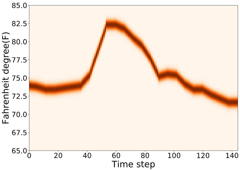
The feasible region of $T^{oa}$ is set to $[65,85]$, which has at least $6\sigma$-wide margins on both sides to the range of the predicted mean, therefore can be considered sufficient for discretization. The feasible region is equally discretized into 100 segments to obtain the discretized values $\tilde{T}_{t}^{oa}$.

Fig. 4 shows the optimized schedules, where DO is solved according to the predicted mean, RO-2$\sigma$ is solved with 95% confidence interval, of which the robust feasible region at each step is $\phi_{t}=[\mu_{t}-2\sigma,\mu_{t}+2\sigma]$. Similarly, RO-3$\sigma$ is solved with 99.7% confidence interval, of which the robust feasible region at each step is $\phi_{t}=[\mu_{t}-3\sigma,\mu_{t}+3\sigma]$. SP-strict and SP-average are the solutions of SP formulations with temperature constraints defined upon individual scenarios and the average of all scenarios. DRO-0, DRO-1, DRO-2, and DRO-2.5 are the solutions of the proposed DRO methods with Wasserstein radius $\varepsilon$ equal to 0, 1, 2 and 2.5 respectively. It can be observed that the discrepancies among these schedules occur in the early morning around 6-8 am and afternoon around 12-4 pm. The former time span involves the ambient temperature ramping up and room temperature upper bound switching to $76^{\circ}F$, and the later time span involves the TOU step-up and ambient temperature ramping down.

Table III summarizes the performance of the 9 optimal schedules, where the subscripts $reg$ and $ext$ denotes the regular testing set and extreme testing set respectively. It can be observed that DO has the lowest operating cost, but comes with high violations in both testing sets. Its poor robustness is because DO only takes the predicted mean into consideration, but in reality, predictions are never perfect. The two RO solutions with different confidence intervals show strong robustness, especially RO-3$\sigma$ has no violations observed in both testing sets, but it also has the highest cost due to its conservativeness. The robustness of SP-strict is close to RO-2$\sigma$ in that their violation number and mileage are at the same level in both testing sets. Their costs are approximately the same, and the cost of SP-strict is 0.6% lower than RO-3$\sigma$.

The solution of SP-average is less conservative than SP-strict because its temperature constraint is based on the average of all scenarios. The schedule of DRO-0 and SP-average are the same, and they have the same cost and robustness. The DRO method with an ambiguity set radius 0, is essentially an SP problem because the ambiguity set only includes the predicted empirical distribution. The only difference is SP-average is solved in a scenario-based way and DRO-0 is solved in the discretized LP manner. From DRO-0 to DRO-2.5, the conservativeness and cost increase with the increase of $\varepsilon$, as a result, the violation number and mileage decrease. From the feasibility perspective, DRO-2 is already very close to SP-strict and RO-2$\sigma$ in the regular test set, and DRO-2.5 yields similar robustness to SP-strict and RO-2$\sigma$ in the extreme test set. The violation number and mileage of DRO-2.5 even become slightly lower than SP-strict. In terms of optimality, the cost of DRO-2 is 6.6% lower than SP-strict and RO-2$\sigma$. DRO-2.5 is more expensive than DRO-2 by 2.3% but is cheaper than SP-strict and RO-2$\sigma$ by 4.5%. The cost of DRO solutions with $\varepsilon\in\left(0,2.5\right]$ is bounded by the cost of DRO-0 and DRO-2.5. It can be concluded that, with the proper selection of $\varepsilon$, the proposed DRO method can provide competitively robust schedules compared to SP and RO methods with lower costs. The proposed DRO method provides building managers with granular options according to their trade-off between economic and reliability preferences.

References

- [1] EIA, “How much energy is consumed in u.s. residential and commercial buildings? - faq - u.s. energy information administration (eia),” https://www.eia.gov/tools/faqs/faq.php?id=86&t=1, last accessed August 16, 2019.
- [2] N. Lu, “An evaluation of the hvac load potential for providing load balancing service,” IEEE Transactions on Smart Grid, vol. 3, no. 3, pp. 1263–1270, 2012.
- [3] G. Goddard, J. Klose, and S. Backhaus, “Model development and identification for fast demand response in commercial hvac systems,” IEEE Transactions on Smart Grid, vol. 5, no. 4, pp. 2084–2092, 2014.
- [4] “Google nest learning thermostat,” https://nest.com/thermostats/real-savings/, last accessed Oct 06, 2020.
- [5] “Simple, powerful, cloud-based energy management,” https://www.ecobee.com/smartbuildings/how-it-works/, last accessed Oct 06, 2020.
- [6] “Honeywell T9 smart thermostat with sensor,” https://www.honeywellhome.com/us/en/products/air/thermostats/wifi-thermostats/t9-smart-thermostat-with-sensor-rcht9610wfsw2003-u/, last accessed Oct 06, 2020.
- [7] W. Tian, Y. Heo, P. De Wilde, Z. Li, D. Yan, C. S. Park, X. Feng, and G. Augenbroe, “A review of uncertainty analysis in building energy assessment,” Renewable and Sustainable Energy Reviews, vol. 93, pp. 285–301, 2018.
- [8] B. J. Moore and D. S. Fisher, “Pump differential pressure setpoint reset based on chilled water valve position,” ASHRAE Transactions, vol. 109, p. 373, 2003.
- [9] H. Mirinejad, S. H. Sadati, M. Ghasemian, and H. Torab, “Control techniques in heating, ventilating and air conditioning (hvac) systems 1,” 2008.
- [10] D. S. Naidu and C. G. Rieger, “Advanced control strategies for heating, ventilation, air-conditioning, and refrigeration systems—an overview: Part i: Hard control,” Hvac&R Research, vol. 17, no. 1, pp. 2–21, 2011.
- [11] F. Engdahl and D. Johansson, “Optimal supply air temperature with respect to energy use in a variable air volume system,” Energy and Buildings, vol. 36, no. 3, pp. 205–218, 2004.
- [12] S. Wang and Z. Ma, “Supervisory and optimal control of building hvac systems: A review,” Hvac&R Research, vol. 14, no. 1, pp. 3–32, 2008.
- [13] J. I. Levenhagen and D. H. Spethmann, HVAC controls and systems. McGraw-Hill New York, 1993.
- [14] S. Qiu, F. Feng, W. Zhang, Z. Li, and Z. Li, “Stochastic optimized chiller operation strategy based on multi-objective optimization considering measurement uncertainty,” Energy and Buildings, vol. 195, pp. 149–160, 2019.
- [15] Y. Du, L. Jiang, C. Duan, Y. Li, and J. Smith, “Energy consumption scheduling of hvac considering weather forecast error through the distributionally robust approach,” IEEE Transactions on Industrial Informatics, vol. 14, no. 3, pp. 846–857, 2017.
- [16] G. Tian, S. Faddel, Q. Zhou, Z. Qu, and A. Parlato, “Optimal coordination of hvac scheduling for commercial buildings,” in 2020 IEEE Texas Power and Energy Conference (TPEC). IEEE, 2020, pp. 1–5.
- [17] H. Hao, C. D. Corbin, K. Kalsi, and R. G. Pratt, “Transactive control of commercial buildings for demand response,” IEEE Transactions on Power Systems, vol. 32, no. 1, pp. 774–783, 2016.
- [18] X. Geng and L. Xie, “Data-driven decision making with probabilistic guarantees (part 1): A schematic overview of chance-constrained optimization,” arXiv preprint arXiv:1903.10621, 2019.
- [19] P. M. Esfahani and D. Kuhn, “Data-driven distributionally robust optimization using the wasserstein metric: Performance guarantees and tractable reformulations,” Mathematical Programming, vol. 171, no. 1-2, pp. 115–166, 2018.
- [20] S. Boyd, S. P. Boyd, and L. Vandenberghe, Convex optimization. Cambridge university press, 2004.
- [21] “Duke energy commercial/industrial rate schedules,” https://www.duke-energy.com/_/media/pdfs/rates/peratespefcommercialrateinsert.pdf?la=en, last accessed March 06, 2020.