Fast Beam Training and Alignment for IRS-Assisted Millimeter Wave/Terahertz Systems

We consider the problem of downlink training and beam alignment in an IRS-assisted mmWave/THz multi-user system, where an IRS is deployed to assist the data transmission from the BS to a number of single-antenna users (see Fig. 1).

Before proceeding, we first provide a discussion of our proposed downlink training protocol. In the downlink beam training stage, the BS periodically broadcasts a pre-designed common beam training sequence $\{\boldsymbol{f}(t)\}_{t=1}^{T}$, and at the same time the IRS uses a common reflection beam sequence $\{\boldsymbol{v}(t)\}_{t=1}^{T}$ to reflect the signal coming from the BS. For simplicity, we assume that the direct link from the BS to each user is blocked due to unfavorable conditions, and the transmitted signal arrives at each user via the reflected BS-IRS-user channel¹¹ 1 When the direct link between the BS and the user is available, we can first switch off the IRS and perform downlink training of the direct link using conventional mmWave beam training schemes. The effect of the direct link can then be canceled when we perform downlink BS-IRS-user training.. Each user receives signals reflected from the IRS, and estimates the angular parameters associated with the dominant path of its own downlink channel. This information is then sent by this user to the BS via a dedicated channel. A connection can thus be established between the BS and each user after the BS receives the related channel information associated with this user. The schematic of the downlink training protocol is also illustrated in Fig. 2.

In this downlink training framework, we are interested in studying how to jointly devise the active/passive beam training sequences and estimate the channel parameters to achieve fast beam alignment between the BS and each user. Note that since channel estimation is performed at each user and the design of beam training sequences is independent of users, our study can be simplified to single-user scenarios. Therefore in the rest of the paper, we consider the scenario where there is only a single user in the system. Also, in our setup, we assume that the BS has no knowledge of the geographical location of all facilities, including the IRS, the user and the BS itself.

To more rigorously formulate our problem, we now proceed to discuss our system model. The BS is equipped with $N_{t}$ antennas and $R\ll N_{t}$ radio frequency (RF) chains. At the BS, a digital baseband precoder $\boldsymbol{f}_{\text{BB}}\in\mathbb{C}^{R}$ is first applied to a broadcast signal ${s}$, then followed by an analog RF beamformer $\boldsymbol{F}_{\text{RF}}\in\mathbb{C}^{N_{t}\times R}$. The transmitted training signal at the $t$th time instant can be written as

where $\boldsymbol{f}(t)\triangleq\boldsymbol{F}_{\text{RF}}(t)\boldsymbol{f}_{\text{BB}}(t)$ is the transmitter’s beamforming vector, and we set $s(t)=1$ in the beam training stage. Let $\boldsymbol{G}\in\mathbb{C}^{M\times N_{t}}$ denote the channel from the BS to the IRS, and $\boldsymbol{h}_{r}\in\mathbb{C}^{M}$ denote the channel from the IRS to the user. The IRS is a planar array consisting of $M=M_{y}\times M_{z}$ passive reflecting elements. Each reflecting element of the IRS can reflect the incident signal with a reconfigurable phase shift and amplitude via a smart controller. Let $\phi_{m}(t)\in[0,2\pi]$ and $\zeta_{m}(t)\in[0,1]$ denote the phase shift and amplitude coefficients adopted by the $m$th element at the $t$th time instant. Define

as the IRS reflecting matrix. The training signal received by the user can thus be expressed as

where $\boldsymbol{v}(t)\triangleq[\zeta_{1}(t)e^{j\phi_{1}(t)}\phantom{0}\cdots\phantom{0}\zeta_{M}(t)e^{j\phi_{M}(t)}]^{H}$ is the passive reflecting vector, $\boldsymbol{H}\triangleq{\rm diag}(\boldsymbol{h}_{r}^{H})\boldsymbol{G}\in\mathbb{C}^{M\times N_{t}}$ is referred to as the cascade channel, and $n(t)\sim\mathcal{CN}(0,\sigma^{2})$ represents the additive white Gaussian noise.

It is well-known that the narrowband mmWave channel can be characterized by a widely-used Saleh-Valenzuela (S-V) geometric model [32, 33]. As for THz channels, some initial channel measurements at THz frequencies [34, 35, 36, 37] reported that THz channels also exhibit sparse scattering characteristics, an effect that is observable at mmWave frequencies. The main difference between the mmWave and THz channels lies in the path loss. Specifically, THz channels suffer more severe free spreading loss due to the extremely high frequency. In addition, the high attenuation caused by molecular absorption is no longer negligible and has to be taken into account at THz frequencies. On the other hand, due to the severe path loss of THz frequencies, THz channels may exhibit a higher degree of sparsity than mmWave communications. As a result, THz channels can also be characterized by the S-V model. Specifically, the BS-IRS channel can be modeled as

where $P$ is the total number of paths between the BS and the IRS, $\varrho_{0}$ denotes the complex gain of the LOS path, $\varrho_{p},\forall p=1,\ldots,P-1$ represents the complex gain of the $p$th NLOS path, $\vartheta_{p}^{r}$ ($\gamma_{p}^{r}$) for $p=0,1,\ldots,P-1$ denotes the associated azimuth (elevation) AoA, $\phi_{p}^{t}$ for $p=0,\ldots,P-1$ is the associated AoD, and $\boldsymbol{a}_{r}$ ($\boldsymbol{a}_{t}$) denotes the normalized receive (transmit) array response vector. For simplicity, we define

Suppose the BS employs a uniform linear array (ULA). The transmit array response vector can be expressed as

Also, since the IRS is an $M_{y}\times M_{z}$ uniform planar array, the receive array response vector can be written as

where $\otimes$ denotes the Kronecker-product, $d$ is the antenna spacing and $\lambda$ denotes the wavelength of the signal.

Owing to the sparse scattering nature of mmWave channels, the BS-IRS channel has a sparse representation in the angular (beam-space) domain:

where $\boldsymbol{D}_{\rm R}\triangleq\boldsymbol{D}_{M_{y}}\otimes\boldsymbol{D}_{M_{z}}\in\mathbb{C}^{M\times M}$, $\boldsymbol{D}_{M_{y}}$, $\boldsymbol{D}_{M_{z}}$, and $\boldsymbol{D}_{N_{t}}$ are defined as

with $N=M_{y},M_{z},N_{t}$ respectively, $\eta(i)=-1+\frac{2i-1}{N},i=1,\ldots,N$, and $\boldsymbol{\Sigma}\in\mathbb{C}^{M\times N_{t}}$ is a sparse matrix with $P$ nonzero entries. Here we suppose that the true AoA and AoD lie on the discretized grid. In the presence of grid mismatch, the number of nonzero elements in the sparse matrix will increase as a result of power leakage.

Similarly, the IRS-user channel can be modeled as

where $P^{\prime}$ is the number of signal paths between the IRS and the user, $\alpha_{0}$ denotes the complex gain of the LOS path, $\alpha_{p},\forall p=1,\ldots,P^{\prime}-1$ denotes the complex gain associated with the $p$th NLOS path, and $\vartheta_{p}^{t}$ ($\gamma_{p}^{t}$) for $p=0,1,\ldots,P^{\prime}-1$ denotes the associated azimuth (elevation) AoD. Due to sparse scattering characteristics, the IRS-user channel can be written as

where $\boldsymbol{\alpha}\in\mathbb{C}^{M\times 1}$ is a sparse vector with $P^{\prime}$ nonzero entries. It is easy to verify that $\boldsymbol{D}_{\rm R}^{H}\boldsymbol{D}_{\rm R}=\boldsymbol{I}_{M}$ and $\boldsymbol{D}_{N_{t}}^{H}\boldsymbol{D}_{N_{t}}=\boldsymbol{I}_{N_{t}}$.

Based on (8) and (11), it was shown in [13] that the cascade channel admits a sparse representation as follows

where $\boldsymbol{\bar{D}}_{R}\triangleq\boldsymbol{\tilde{D}}_{R}(:,1:M)$ is a submatrix of $\boldsymbol{\tilde{D}}_{R}$ constructed by its first $M$ columns, and $\boldsymbol{\tilde{D}}_{R}\triangleq\sqrt{M}\boldsymbol{D}_{\rm R}^{\ast}\bullet\boldsymbol{D}_{\rm R}$, with $\bullet$ denoting the transposed Khatri-Rao product. It can be readily verified that $\boldsymbol{\tilde{D}}_{R}\in\mathbb{C}^{M\times M^{2}}$ has $M$ distinct columns which are exactly its first $M$ columns. Also, we can verify that $\boldsymbol{\bar{D}}_{R}$ is an unitary matrix, i.e. $\boldsymbol{\bar{D}}_{R}^{H}\boldsymbol{\bar{D}}_{R}=\boldsymbol{I}_{M}$, and its column takes the form of $\boldsymbol{\bar{a}}_{r}(\varphi,\varpi)\triangleq\boldsymbol{a}(\varphi,M_{y})\otimes\boldsymbol{a}(\varpi,M_{z})$.

Also, we have

in which $\boldsymbol{\tilde{\Lambda}}$ is a merged version of $\boldsymbol{J}\triangleq\boldsymbol{\alpha}^{\ast}\otimes\boldsymbol{\Sigma}$, with each of its rows being a superposition of a subset of rows in $\boldsymbol{J}$, i.e.

where $\boldsymbol{\tilde{\Lambda}}(i,:)$ denotes the $i$th row of $\boldsymbol{\tilde{\Lambda}}$, $\mathcal{S}_{i}$ denotes the set of indices associated with those columns in $\boldsymbol{\tilde{D}}_{R}$ that are identical to the $i$th column of $\boldsymbol{\bar{D}}_{R}$. It is clear that $\boldsymbol{\Lambda}$ is a sparse matrix with at most $P\times P^{\prime}$ nonzero elements.

Combining (3) and (12), the received pilot signal at the user can be expressed as

Note that (15) is an ideal signal model without considering the CFO and random phase noise. In mmWave/THz bands, the CFO, i.e., the mismatch in the carrier frequencies at the transmitter and the receiver, is more significant than sub-6GHz bands and cannot be neglected. For instance, a small offset of 10 parts per million (ppm) at mmWave frequencies can cause a large phase misalignment in less than a hundred nanoseconds. Besides the CFO, mmWave communication systems also suffer random phase noise due to the jitter of the oscillators. The phase noise, together with the CFO, leads to an unknown phase shift to measurements $z(t)$ that varies across time. In this case, only the magnitude of the measurement $z(t)$ is reliable. Define

Based on $\{y(t)\}_{t=1}^{T}$, our objective is to acquire the information needed to achieve beam alignment between the BS and the user. Note that identifying the best beam alignment is equivalent to acquiring the location index of the largest (in magnitude) element in the sparse matrix $\boldsymbol{\Lambda}$. This is because $\boldsymbol{\Lambda}$ is a beam-space representation of the cascade channel $\boldsymbol{H}$. Hence the largest element in $\boldsymbol{\Lambda}$ actually corresponds to the strongest path of the BS-IRS-user channel.

To identify the largest element in $\boldsymbol{\Lambda}$, a natural approach is to exhaustively search all possible beam pairs. Specifically, at each time instant $t$, choose $\boldsymbol{f}(t)\triangleq\boldsymbol{F}_{\text{RF}}(t)\boldsymbol{f}_{\text{BB}}(t)$ as a certain column from $\boldsymbol{D}_{N_{t}}$, and choose $\boldsymbol{v}(t)$ as a certain column from $\boldsymbol{\bar{D}}_{R}$, i.e.

Here the scaler $\sqrt{M}$ in $\boldsymbol{v}(t)$ is used to ensure that entries of $\boldsymbol{v}(t)$ are of constant modulus. Then the received measurement $y(t)$ is given by

where $\lambda_{i,j}$ denotes the $(i,j)$th entry of $\boldsymbol{\Lambda}$. After an exhaustive search, we can identify the largest (in magnitude) entry in $\boldsymbol{\Lambda}$. This exhaustive search scheme, however, has a sample complexity of $MN_{t}$, which is prohibitively high since both $M$ and $N_{t}$ are large for mmWave and THz systems in order to combat severe path loss. In the following sections, we develop a more efficient method to perform joint BS-IRS-user beam training.

Specifically, since the period of time for beam training is proportional to the number of measurements $T$, the problem of interest is how to devise the active/passive beam training sequences $\{\boldsymbol{f}(t),\boldsymbol{v}(t)\}_{t=1}^{T}$ and develop a computationally efficient estimation scheme such that we can identify the best beam alignment using as few measurements as possible.

Remark: Different from our work that neglects the phase information of the received measurements, we noticed that some other works, e.g. [18, 17], model the CFO as an unknown parameter and perform joint CFO and channel estimation.

In this subsection, we discuss how to devise a set of sparse sensing vectors $\{\boldsymbol{c}(t),\boldsymbol{a}(t)\}_{t=1}^{T}$ to efficiently probe the channel. Let $S_{c}(t)\triangleq\{i|c_{i}(t)>0\}$ denote the set of indices associated with the nonzero elements in $\boldsymbol{c}(t)$, and $S_{a}(t)\triangleq\{j|a_{j}(t)>0\}$ denote the set of indices of the nonzero elements in $\boldsymbol{a}(t)$. Also, for simplicity, we assume that the nonzero entries in $\{\boldsymbol{c}(t)\}$ are all set to $\beta>0$, and the nonzero entries in $\{\boldsymbol{a}(t)\}$ are all set to $\gamma>0$. Therefore, we have

To find the strongest signal path, we need to make sure that each element in $\boldsymbol{\Lambda}$ will be scanned at least once. We first introduce the concept of “a round of full-coverage scanning” as a basic building block for our beam training process. Define $U\triangleq M/Q$ and $V\triangleq N_{t}/R$ and assume both of them are integers. Each round of full-coverage scanning consists of $T_{0}=U\times V$ measurements, and these $T_{0}$ measurements are generated according to:

where $\boldsymbol{C}\in\mathbb{R}^{M\times U}$, $\boldsymbol{A}\in\mathbb{R}^{N_{t}\times V}$, and $\boldsymbol{Y}\in\mathbb{R}^{U\times V}$ is a matrix constructed by $\{y(t)\}_{t=1}^{T_{0}}$. Specifically, the $(u,v)$th entry of $\boldsymbol{Y}$ is equal to $\boldsymbol{Y}(u,v)=y((u-1)V+v)$, and $(u,v)$th entry of $\boldsymbol{N}$ is equal to $\boldsymbol{N}(u,v)=n((u-1)V+v)$. Therefore, once $\boldsymbol{C}$ and $\boldsymbol{A}$ are specified, the set of sparse sensing vectors $\{\boldsymbol{c}(t),\boldsymbol{a}(t)\}_{t=1}^{T_{0}}$ can be accordingly determined. Let

From the relation between $\boldsymbol{Y}$ and $\{y(t)\}$, it is clear that we have $\boldsymbol{c}_{u}=\boldsymbol{c}((u-1)V+v),\forall v$ and $\boldsymbol{a}_{v}=\boldsymbol{a}((u-1)V+v),\forall u$. The set of sparse encoding vectors $\{\boldsymbol{c}_{u}\}$ and $\{\boldsymbol{a}_{v}\}$ are devised to satisfy the following two conditions:

• C1

  Those nonzero entries in $\{\boldsymbol{c}_{u}\}$ and $\{\boldsymbol{a}_{v}\}$ are respectively set to $\beta$ and $\gamma$. Also, we have $\|\boldsymbol{c}_{u}\|_{0}=Q,\forall u$, and $\|\boldsymbol{a}_{v}\|_{0}=R,\forall v$.

• C2

  The sparse vectors in $\{\boldsymbol{c}_{u}\}$ are orthogonal to each other, i.e. $\boldsymbol{c}_{u_{1}}^{T}\boldsymbol{c}_{u_{2}}=0,\forall u_{1}\neq u_{2}$; and vectors in $\{\boldsymbol{a}_{v}\}$ are orthogonal to each other, i.e. $\boldsymbol{a}_{v_{1}}^{T}\boldsymbol{a}_{v_{2}}=0,\forall v_{1}\neq v_{2}$.

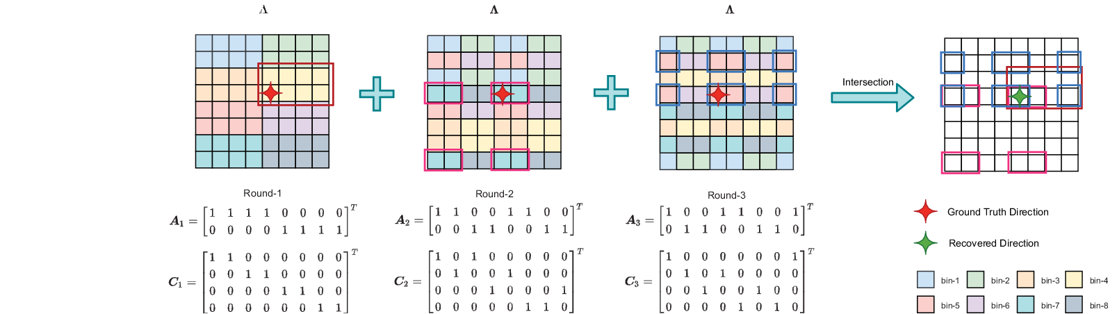
Let $S(t)\triangleq\{\lambda_{i,j}\}_{i\in S_{c}(t),j\in S_{a}(t)}$ denote the set of elements that are simultaneously sensed/hashed at the $t$th time instant. Such a set of elements is also called as a bin, as illustrated in Fig. 3. Clearly we have $|S(t)|=QR$. Also, condition C2 ensures that the sets of elements sensed at different time instants are disjoint, i.e.

In addition, since we have $UQ=M$ and $RV=N_{t}$, the union of the sets is equal to the whole set of elements of $\boldsymbol{\Lambda}$, i.e.

After a single round of full-coverage scanning, no element in $\boldsymbol{\Lambda}$ is left unscanned. Nevertheless, since each element in $\boldsymbol{\Lambda}$ is scanned along with other elements at each time, we still cannot identify the exact location of the largest component from the measurements $\boldsymbol{Y}$. To identify the strongest component, we need to perform a few rounds, say $L$ rounds, of full-coverage scanning, and for each round of scanning, we randomly generate $\boldsymbol{A}$ and $\boldsymbol{C}$ by altering locations of the nonzero entries in $\{\boldsymbol{c}_{u}\}$ and $\{\boldsymbol{a}_{v}\}$. We will show that we can identify the largest element in $\boldsymbol{\Lambda}$ via a simple decoding scheme from these $L$ rounds of measurements $\{\boldsymbol{Y}_{l}\}_{l=1}^{L}$. Here $\boldsymbol{Y}_{l}$ denotes the measurement matrix collected at the $l$th round of scanning, and we have

where $\boldsymbol{C}_{l}\triangleq[\boldsymbol{c}^{l}_{1}\phantom{0}\ldots\phantom{0}\boldsymbol{c}^{l}_{U}]$ and $\boldsymbol{A}_{l}\triangleq[\boldsymbol{a}^{l}_{1}\phantom{0}\ldots\phantom{0}\boldsymbol{a}^{l}_{V}]$ are sparse encoding matrices used in the $l$th round of scanning.

As discussed in the previous subsection, the vectors $\{\boldsymbol{c}_{u}\}$ are devised to be strictly sparse with $Q$ nonzero elements. To fulfill this requirement, we need to have an independent control of the reflection amplitude for each IRS element, which increases not only the hardware complexity but also the energy consumption [38, 39]. Moreover, to generate a strictly sparse vector $\boldsymbol{c}_{u}$, many of the reflection amplitudes have to be set far less than one, which reduces the reflection efficiency.

To cope with these issues, we wish to find a set of passive beamforming vectors $\{\boldsymbol{v}_{u}\}$ with constant modulus, and the corresponding vectors $\{\boldsymbol{c}_{u}=\boldsymbol{\bar{D}}_{R}^{H}\boldsymbol{v}_{u}\}$ are approximately-sparse vectors with $Q$ dominant entries. Mathematically, this problem can be formulated as follows. Given any $Q$ columns from $\boldsymbol{\bar{D}}_{R}$, denoted as $\{\boldsymbol{p}_{q}\}_{q=1}^{Q}$, let $\boldsymbol{Q}$ be a matrix constructed by these $Q$ columns and $\boldsymbol{\bar{Q}}$ be a matrix obtained by removing those $Q$ columns from $\boldsymbol{\bar{D}}_{R}$. We seek a constant-modulus vector $\boldsymbol{v}$ such that $|\boldsymbol{v}^{H}\boldsymbol{Q}|$ is a quasi-constant magnitude vector with its magnitude as large as possible, whereas $\|\boldsymbol{v}^{H}\boldsymbol{\bar{Q}}\|_{2}$ is as small as possible. There are different approaches to tackle this problem. Inspired by [6], here we formulate the above problem into the following optimization:

where $v_{i}$ denotes the $i$th entry of the vector $\boldsymbol{v}$. It was shown in [6] that the solution to (29) is nearly orthogonal to $\boldsymbol{\bar{Q}}$. Moreover, entries of the vector $\boldsymbol{v}^{H}\boldsymbol{Q}$ have quasi-constant magnitudes thanks to the logarithmic function. As a result, the resulting vector $\boldsymbol{c}=\boldsymbol{\bar{D}}_{R}^{H}\boldsymbol{v}$ is an approximately sparse vector with $Q$ dominant entries. Note that the generated vectors $\{\boldsymbol{c}_{u}\}$ cannot be strictly orthogonal to each other since they are no longer strictly sparse vectors. Nevertheless, for each round of full-coverage scanning, it is not difficult to attain near-orthogonality by making sure that the sets of dominant elements sensed at different time instants are disjoint. Also, as will be shown later in this paper, our proposed algorithm requires the indices of those nonzero elements in $\{\boldsymbol{c}_{u}\}$ to identify the best alignment. As $\{\boldsymbol{c}_{u}\}$ generated from (29) are approximately sparse, we only consider these $Q$ prominent entries as nonzero elements of $\boldsymbol{c}_{u}$.

The above optimization can be efficiently solved by a manifold-based algorithm, which has a very low computational complexity of $\mathcal{O}(M)$ [6]. Besides, the reflecting vectors $\{\boldsymbol{v}_{u}\}$ can be calculated and stored in advance. It will not exert an extra computational burden on the beam alignment task.

We now analyze the sample complexity of the proposed scheme. To ensure that we can recover the index of the dominant element of $\boldsymbol{\Lambda}$ with a probability exceeding a predefined threshold $p_{0}$, we need

For simplicity, we set $p_{0}=p_{1}\times p_{2}$, and let

From (37), it is easy to verify that

where $c_{1}\triangleq\log(({1-p_{1}})^{-1})>0$ is a constant. On the other hand, from (38), we have

where $c_{2}=\log(({1-p_{2}})^{-1})$ is a constant.

Therefore, the total number of measurements $T$ required for identifying the strongest component with a probability at least $p_{0}$ can be calculated as

Since $L_{1}$ ($L_{2}$) is in the order of $\mathcal{O}(\log(M))$ ($\mathcal{O}(\log(N_{t}))$), the proposed intersection-based scheme has a sample complexity of $\mathcal{O}(UV\max\{\log(M),\log(N_{t})\})$. Recall that $U=M/Q$, where $Q$ is a parameter of user’s choice. Thus, we can choose a proper $Q$ to obtain a small value of $U$. To be specific, given $T$ and other system parameters, we can try different combinations of $(Q,L)$ to determine the one which yields the highest probability of correct beam alignment. Here we provide an example to show how many measurements are exactly required to achieve perfect beam alignment with a decent probability. Suppose $N_{t}=128$, $M=256$, $R=4$. For different choice of $Q$ and $L$, our proposed method can identify the best beam alignment with a probability no less than:

• •

  $Q=32$, $L=4$, $T=UVL=1024$: ${\rm P}\geq 94.43\%$

• •

  $Q=16$, $L=3$, $T=UVL=1536$: ${\rm P}\geq 94.65\%$

• •

  $Q=16$, $L=4$, $T=UVL=2048$: ${\rm P}\geq 99.69\%$

From this example, we see that the proposed scheme can achieve a substantial training overhead reduction as compared with the exhaustive search scheme which requires a total number of measurements up to $T=MN_{t}=32768$.

The proposed intersection scheme may not work well in the presence of noise. In the sequel, inspired by [24], we develop a noisy version of the intersection scheme. The basic idea is to assign each element in $\boldsymbol{\Lambda}$ a probability instead of a $0/1$-hard vote, and turn the intersection operation into a product of probabilities.

Specifically, for each round of scanning and each index $(i,j)$ of the element in $\boldsymbol{\Lambda}$, we define an indicator matrix, $\boldsymbol{I}^{(l)}_{(i,j)}\in\mathbb{\{}0,1\}^{U\times V}$, with its $(u,v)$th entry defined as

where $\boldsymbol{x}(j)$ denotes the $j$th element of the vector $\boldsymbol{x}$. Clearly, if the element $\boldsymbol{\Lambda}(i,j)$ is sensed at the time instant $((u-1)V+v)$ of the $l$th round, the value in (42) would be $1$; otherwise it would be $0$.

Based on the indicator matrix, we can further calculate the “probability” matrix $\boldsymbol{\mathcal{P}}^{(l)}$ with its $(i,j)$th entry defined as

where ${\text{vec}}(\cdot)$ denotes the vectorization operator and $\circ$ represents the Hadamard product. Here (43) uses the received magnitude measurement as a weight to calculate the probability of the element $\boldsymbol{\Lambda}(i,j)$ being a dominant entry in $\boldsymbol{\Lambda}$.

Generally, if $\boldsymbol{\mathcal{P}}^{(l)}({i,j})\geq\epsilon$, where $\epsilon$ is a pre-specified threshold, then $(i,j)$ is regarded as a candidate index of the dominant entry in $\boldsymbol{\Lambda}$. Let $\mathcal{F}_{l}=\{(i,j)|\boldsymbol{\mathcal{P}}^{(l)}({i,j})\geq\epsilon\}$ denote the set of candidate indices obtained from the $l$th round. After $L$ rounds of scanning, we can determine the location index of the dominant entry $(i^{\ast},j^{\ast})$ via a maximum likelihood (ML) estimation

where $\mathcal{F}\triangleq\cup_{l=1}^{L}\mathcal{F}_{l}$ denotes the set comprising all candidate indices. The overall algorithm for LOS scenarios are summarized in Algorithm 1.

The major computational task of our proposed beam estimation method is to calculate the probability matrix defined in (43). According to (43), each entry of the probability matrix is calculated as an inner product of two $UV$-dimensional vectors. Since each element in $\boldsymbol{\Lambda}$ is sensed only once in each round, the indicator matrix $\boldsymbol{I}^{(l)}_{(i,j)}$ contains only one nonzero entry. Therefore each entry of the probability matrix can be calculated by multiplying this nonzero entry with its corresponding entry in ${\text{vec}}(\boldsymbol{Y}_{l}\circ\boldsymbol{Y}_{l}^{\ast})$. As a result, calculating this entire probability matrix $\boldsymbol{\mathcal{P}}^{(l)}\in\mathbb{R}^{M\times N_{t}}$ involves a computational complexity of $\mathcal{O}(MN_{t})$. Note that our proposed method requires to compute a set of probability matrices $\{\boldsymbol{\mathcal{P}}^{(l)}\}_{l=1}^{L}$, which has a computational complexity in the order of $\mathcal{O}(MN_{t}L)$, where $L$ is the number of rounds of full-coverage scanning. After obtaining $\{\boldsymbol{\mathcal{P}}^{(l)}\}_{l=1}^{L}$, we need to calculate the objective function defined in (44), which is a Hadamard product of the set of probability matrices $\{\boldsymbol{\mathcal{P}}^{(l)}\}_{l=1}^{L}$ and involves a computational complexity of $\mathcal{O}(MN_{t}(L-1))$. From the above discussion, we see that the overall computational complexity of our proposed method is in the order of $\mathcal{O}(MN_{t}L)$.

As a comparison, as analyzed in [13], if we employ a compressed sensing-based method to recover the cascade channel, the method needs to solve a sparse signal recovery problem of size $T\times(MN_{t})$, whose computational complexity is of $\mathcal{O}(MN_{t}T\bar{K})$ for greedy methods and of $\mathcal{O}(M^{3}N_{t}^{3})$ for more sophisticated methods such as the basis pursuit. Here $T$ denotes the number of measurements used for channel estimation, and $\bar{K}$ is the sparsity level of the cascade channel matrix. Our analysis shows that for our proposed method, only a few rounds of full-coverage scanning (say, $L<10$) are sufficient to identify the best beam alignment with a probability close to $1$. Hence generally we have $L\ll T\bar{K}$. Therefore, our proposed method has a much lower complexity even compared with the least computationally demanding compressed sensing method.

From the above discussion, we see that our proposed method relies on those measurements collected within the NM rounds of scanning to find the best beam alignment. A natural question is: how likely a round of full-coverage scanning is an NM-round of scanning? We have the following results regarding this question.

References

- [1] J. Zhang, E. Björnson, M. Matthaiou, D. W. K. Ng, H. Yang, and D. J. Love, “Prospective multiple antenna technologies for beyond 5G,” IEEE J. Sel. Areas Commun., vol. 38, no. 8, pp. 1637–1660, Aug. 2020.
- [2] X. Tan, Z. Sun, D. Koutsonikolas, and J. M. Jornet, “Enabling indoor mobile millimeter-wave networks based on smart reflect-arrays,” in Proc. IEEE Int. Conf. Comput. Commun. (INFOCOM), Honolulu, Hawaii, Apr. 15-19 2018, pp. 270–278.
- [3] P. Wang, J. Fang, X. Yuan, Z. Chen, H. Duan, and H. Li, “Intelligent reflecting surface-assisted millimeter wave communications: Joint active and passive precoding design,” IEEE Trans. Veh. Technol., vol. 69, no. 12, pp. 14 960–14 973, Dec. 2020.
- [4] N. S. Perović, M. Di Renzo, and M. F. Flanagan, “Channel capacity optimization using reconfigurable intelligent surfaces in indoor mmwave environments,” in Proc. IEEE Int. Conf. Commun. (ICC), Jun. 7-11 2020, pp. 1–7.
- [5] Q. Wu and R. Zhang, “Intelligent reflecting surface enhanced wireless network via joint active and passive beamforming,” IEEE Trans. Wireless Commun., vol. 18, no. 11, pp. 5394–5409, Nov. 2019.
- [6] P. Wang, J. Fang, L. Dai, and H. Li, “Joint transceiver and large intelligent surface design for massive MIMO mmwave systems,” IEEE Trans. Wireless Commun., vol. 20, no. 2, pp. 1052–1064, Feb. 2021.
- [7] X. Yu, D. Xu, and R. Schober, “MISO wireless communication systems via intelligent reflecting surfaces,” in Proc. IEEE/CIC Int. Conf. Commun. China (ICCC), Aug. 2019, pp. 735–740.
- [8] B. Ning, Z. Chen, W. Chen, and J. Fang, “Beamforming optimization for intelligent reflecting surface assisted MIMO: A sum-path-gain maximization approach,” IEEE Wireless Commun. Lett., vol. 9, no. 7, pp. 1105–1109, Jul. 2020.
- [9] S. Zhang and R. Zhang, “Capacity characterization for intelligent reflecting surface aided MIMO communication,” IEEE J. Sel. Areas Commun., vol. 38, no. 8, pp. 1823–1838, Aug. 2020.
- [10] D. Mishra and H. Johansson, “Channel estimation and low-complexity beamforming design for passive intelligent surface assisted MISO wireless energy transfer,” in Proc. IEEE Int. Conf. Acoust. Speech Signal Process. (ICASSP), Brighton,UK, May 12-17 2019, pp. 4659–4663.
- [11] T. L. Jensen and E. De Carvalho, “An optimal channel estimation scheme for intelligent reflecting surfaces based on a minimum variance unbiased estimator,” in Proc. IEEE Int. Conf. Acoust., Speech Signal Process. (ICASSP), May, 2020, pp. 5000–5004.
- [12] X. Guan, Q. Wu, and R. Zhang, “Anchor-assisted channel estimation for intelligent reflecting surface aided multiuser communication,” IEEE Trans. Wireless Commun., 2021, [Online]. Available: https://arxiv.org/abs/2102.10886.
- [13] P. Wang, J. Fang, H. Duan, and H. Li, “Compressed channel estimation and joint beamforming for intelligent reflecting surface-assisted millimeter wave systems,” IEEE Signal Process. Lett., vol. 27, pp. 905–909, May 2020.
- [14] J. Chen, Y.-C. Liang, H. V. Cheng, and W. Yu, “Channel estimation for reconfigurable intelligent surface aided multi-user MIMO systems,” 2019 [Online]. Available: https://arxiv.org/abs/1912.03619.
- [15] Z.-Q. He and X. Yuan, “Cascaded channel estimation for large intelligent metasurface assisted massive MIMO,” IEEE Wireless Commun. Lett., vol. 9, no. 2, pp. 210–214, Feb. 2019.
- [16] S. Liu, Z. Gao, J. Zhang, M. Di Renzo, and M.-S. Alouini, “Deep denoising neural network assisted compressive channel estimation for mmwave intelligent reflecting surfaces,” IEEE Trans. Veh. Technol., vol. 69, no. 8, pp. 9223–9228, Aug. 2020.
- [17] N. J. Myers and R. W. Heath, “A compressive channel estimation technique robust to synchronization impairments,” in 2017 IEEE 18th Int. Workshop Signal Process. Advances Wireless Commun. (SPAWC). IEEE, Jul. 2017, pp. 1–5.
- [18] N. J. Myers, A. Mezghani, and R. W. Heath, “Swift-link: A compressive beam alignment algorithm for practical mmwave radios,” IEEE Trans. Signal Process., vol. 67, no. 4, pp. 1104–1119, Feb. 2019.
- [19] N. J. Myers and R. W. Heath, “Message passing-based joint CFO and channel estimation in mmwave systems with one-bit ADCs,” IEEE Trans. Wireless Commun., vol. 18, no. 6, pp. 3064–3077, Jun. 2019.
- [20] T. Van Chien, H. Q. Ngo, S. Chatzinotas, M. Di Renzo, and B. Ottersten, “Reconfigurable intelligent surface-assisted cell-free massive MIMO systems over spatially-correlated channels,” Apr. 2021, [Online]. Available: https://arxiv.org/abs/2104.08648.
- [21] A. Alkhateeb, O. El Ayach, G. Leus, and R. W. Heath, “Channel estimation and hybrid precoding for millimeter wave cellular systems,” IEEE J. Sel. Topics Signal Process., vol. 8, no. 5, pp. 831–846, Oct. 2014.
- [22] Z. Xiao, T. He, P. Xia, and X.-G. Xia, “Hierarchical codebook design for beamforming training in millimeter-wave communication,” IEEE Trans. Wireless Commun., vol. 15, no. 5, pp. 3380–3392, May. 2016.
- [23] S. Noh, M. D. Zoltowski, and D. J. Love, “Multi-resolution codebook and adaptive beamforming sequence design for millimeter wave beam alignment,” IEEE Trans. Wireless Commun., vol. 16, no. 9, pp. 5689–5701, Sept. 2017.
- [24] H. Hassanieh, O. Abari, M. Rodriguez, M. Abdelghany, D. Katabi, and P. Indyk, “Fast millimeter wave beam alignment,” in Proc. ACM Spec. Interest Group Data Commun., Budapest, Hungary, Aug. 2018, pp. 432–445.
- [25] W. Wu, N. Cheng, N. Zhang, P. Yang, W. Zhuang, and X. Shen, “Fast mmwave beam alignment via correlated bandit learning,” IEEE Trans. Wireless Commun., vol. 18, no. 12, pp. 5894–5908, Dec. 2019.
- [26] X. Li, J. Fang, H. Duan, Z. Chen, and H. Li, “Fast beam alignment for millimeter wave communications: A sparse encoding and phaseless decoding approach,” IEEE Trans. Signal Process., vol. 67, no. 17, pp. 4402–4417, Sept. 2019.
- [27] B. Ning, Z. Chen, W. Chen, Y. Du, and J. Fang, “Terahertz multi-user massive MIMO with intelligent reflecting surface: Beam training and hybrid beamforming,” IEEE Trans. Veh. Technol., vol. 70, no. 2, pp. 1376–1393, Feb. 2021.
- [28] C. You, B. Zheng, and R. Zhang, “Fast beam training for IRS-assisted multiuser communications,” IEEE Wireless. Commun. Lett., vol. 9, no. 11, pp. 1845–1849, Nov. 2020.
- [29] W. Wang and W. Zhang, “Joint beam training and positioning for intelligent reflecting surfaces assisted millimeter wave communications,” IEEE Trans. Wireless Commun., 2021.
- [30] X. Hu, C. Zhong, Y. Zhu, X. Chen, and Z. Zhang, “Programmable metasurface-based multicast systems: Design and analysis,” IEEE J. Sel. Areas Commun., vol. 38, no. 8, pp. 1763–1776, Aug. 2020.
- [31] H. Wang, J. Fang, P. Wang, G. Yue, and H. Li, “Efficient beamforming training and channel estimation for millimeter wave OFDM systems,” IEEE Trans. Wireless Commun., vol. 20, no. 5, pp. 2805–2819, May 2021.
- [32] O. E. Ayach, S. Rajagopal, S. Abu-Surra, Z. Pi, and R. W. Heath, “Spatially sparse precoding in millimeter wave MIMO systems,” IEEE Trans. Wireless Commun., vol. 13, no. 3, pp. 1499–1513, Mar. 2014.
- [33] T. Jiang, J. Zhang, M. Shafi, L. Tian, and P. Tang, “The comparative study of S-V model between 3.5 and 28 GHz in indoor and outdoor scenarios,” IEEE Trans. Veh. Technol., vol. 69, no. 3, pp. 2351–2364, Mar. 2020.
- [34] C. Han, A. O. Bicen, and I. F. Akyildiz, “Multi-ray channel modeling and wideband characterization for wireless communications in the terahertz band,” IEEE Trans. Wireless Commun., vol. 14, no. 5, pp. 2402–2412, May 2015.
- [35] C. Lin and G. Y. Li, “Indoor terahertz communications: How many antenna arrays are needed?” IEEE Trans. Wireless Commun., vol. 14, no. 6, pp. 3097–3107, Jun. 2015.
- [36] C. Han, J. M. Jornet, and I. Akyildiz, “Ultra-massive MIMO channel modeling for graphene-enabled terahertz-band communications,” in 2018 IEEE 87th Veh. Technol. Conf. (VTC Spring), 3-6, Jun. 2018, pp. 1–5.
- [37] H. Tataria, M. Shafi, A. F. Molisch, M. Dohler, H. Sjöland, and F. Tufvesson, “6G wireless systems: Vision, requirements, challenges, insights, and opportunities,” Proc. IEEE, vol. 109, no. 7, pp. 1166–1199, Jul. 2021.
- [38] S. Abeywickrama, R. Zhang, Q. Wu, and C. Yuen, “Intelligent reflecting surface: Practical phase shift model and beamforming optimization,” IEEE Trans. Commun., vol. 68, no. 9, pp. 5849–5863, Sept. 2020.
- [39] W. Tang, M. Z. Chen, X. Chen, J. Y. Dai, Y. Han, M. Di Renzo, Y. Zeng, S. Jin, Q. Cheng, and T. J. Cui, “Wireless communications with reconfigurable intelligent surface: Path loss modeling and experimental measurement,” IEEE Trans. Wireless Commun., vol. 20, no. 1, pp. 421–439, Jan. 2021.
- [40] M. R. Akdeniz, Y. Liu, M. K. Samimi, S. Sun, S. Rangan, T. S. Rappaport, and E. Erkip, “Millimeter wave channel modeling and cellular capacity evaluation,” IEEE J. Sel. Areas Commun., vol. 32, no. 6, pp. 1164–1179, Jun. 2014.
- [41] Z. Muhi-Eldeen, L. Ivrissimtzis, and M. Al-Nuaimi, “Modelling and measurements of millimetre wavelength propagation in urban environments,” IET Microw. Antennas & Propag., vol. 4, no. 9, pp. 1300–1309, Sept. 2010.
- [42] S. Priebe, M. Kannicht, M. Jacob, and T. Kürner, “Ultra broadband indoor channel measurements and calibrated ray tracing propagation modeling at THz frequencies,” J. Commun. Netw., vol. 15, no. 6, pp. 547–558, Dec. 2013.