跳到论文正文
W Papers独立论文阅读器 arXiv:2103.05778 论文正文 计算阅读时间 · 0%
引用这篇论文根据当前论文元数据生成,正式投稿前建议核对。


License: arXiv.org perpetual non-exclusive license
arXiv:2103.05778v2 [math-ph] 12 Nov 2021

Second-order fast-slow dynamics of non-ergodic Hamiltonian systems: Thermodynamic interpretation and simulation

Matthias Klar Note: M.Klar@bath.ac.uk Affiliation: Department of Mathematical Sciences, University of Bath, Bath BA2 7AY, United Kingdom    Karsten Matthies Note: K.Matthies@bath.ac.uk Affiliation: Department of Mathematical Sciences, University of Bath, Bath BA2 7AY, United Kingdom    Celia Reina Note: creina@seas.upenn.edu Affiliation: Department of Mechanical Engineering and Applied Mechanics, University of Pennsylvania, Philadelphia PA 19104, USA    Johannes Zimmer Note: jz@ma.tum.de Affiliation: Department of Mathematics, Technische Universität München, Boltzmannstr. 3, 85748 Garching, Germany
Abstract

A class of fast–slow Hamiltonian systems with potential UεU_{\varepsilon} describing the interaction of non-ergodic fast and slow degrees of freedom is studied. The parameter ε\varepsilon indicates the typical timescale ratio of the fast and slow degrees of freedom. It is known that the Hamiltonian system converges for ε→0\varepsilon\to 0 to a homogenised Hamiltonian system. We study the situation where ε\varepsilon is small but positive. First, we rigorously derive the second-order corrections to the homogenised (slow) degrees of freedom. They can be decomposed into explicitly given terms that oscillate rapidly around zero and terms that trace the average motion of the corrections, which are given as the solution to an inhomogeneous linear system of differential equations. Then, we analyse the energy of the fast degrees of freedom expanded to second-order from a thermodynamic point of view. In particular, we define and expand to second-order a temperature, an entropy and external forces and show that they satisfy to leading-order, as well as on average to second-order, thermodynamic energy relations akin to the first and second law of thermodynamics. Finally, we analyse for a specific fast–slow Hamiltonian system the second-order asymptotic expansion of the slow degrees of freedom from a numerical point of view. Their approximation quality for short and long time frames and their total computation time are compared with those of the solution to the original fast–slow Hamiltonian system of similar accuracy.

Keywords:

Two-scale Hamiltonian, Asymptotic expansion, Coarse-graining, Far-from-equilibrium, Many-degrees-of-freedom interaction

1 Introduction

Many scientists in physics, chemistry and materials science resort to computer simulations to study real-world dynamical processes. These simulations open up the possibility to quickly and inexpensively iterate through different experimental setups, thus hugely reducing cost in the form of time and labour and allow a level of insight into small- and large-scale processes that were out of reach decades ago. In chemical physics or materials science, for example, scientists frequently analyse large scale molecular dynamics simulations to predict properties of large dynamical systems based on mathematical models that aim to describe the dynamical evolution of the constituent particles. In simulating these systems, one typically encounters two problems that severely impede their scalability. Firstly, the simulation of molecular structures requires a step size in the numerical integration scheme that ranges in the order of 10−1510^{-15} seconds to accurately replicate the fast molecular vibrations in the system. Secondly, even small macroscopic systems of interest require the integration of a potentially large number of particles. Even more, the two problems often compound and pose a challenging obstacle in the scalability and utility of molecular dynamic simulations.

From an applications point of view, one is often not interested in analysing the exact evolution of the fast molecular vibrations, but in the slow conformal motion that embodies the macroscale dynamics of the system. Here lies an opportunity to bypass at least partly the scalability issues by advancing the understanding of these systems and a subsequent development of numerical integration schemes that describe only the average evolution of the dynamical system without fully resolving the small-scale vibrations.

Fast–slow Hamiltonian systems provide a simplified fundamental description of large-scale interacting particles systems, where the system’s degrees of freedom evolve on different scales in time and space. They can be used, for example, to model the evolution of molecules where the slow degrees of freedom represent the conformal motion and the fast degrees of freedom represent the high-frequency molecular vibrations [3]. There is a vast body of literature for averaging general dynamical systems, not necessarily of Hamiltonian type, for example, using Young measures [6]. Applications of such fast–slow systems arise, for example, in models of plasticity [7]. Recent work on averaging of Hamiltonian fast–slow systems and connections with adiabatic invariants include [16, 19, 20] and references therein. Similar averaging techniques are also relevant to understand equilibration in springy billiards [26]. For general references to averaging, we refer the reader to [24, 15, 21].

With a mathematical description of a dynamical system in the form of a fast–slow Hamiltonian system, we are able to derive the conformal motion through homogenisation in time. The theory laid out by Bornemann in [3] enables us to derive the homogenised evolution of a specific class of fast–slow Hamiltonian systems. More precisely, Bornemann considers a family of mechanical systems, parametrised by a scale parameter ε\varepsilon, whose Lagrangian is of the form

(1) ℒε​(x,x˙)=12​⟨x˙,x˙⟩−Wε​(x),x˙∈Tx​M,\mathscr{L}_{\varepsilon}(x,\dot{x})=\tfrac{1}{2}\left\langle\dot{x},\dot{x}\right\rangle-W_{\varepsilon}(x),\qquad\dot{x}\in T_{x}M,

on a Euclidean configuration space M=ℝmM=\mathbb{R}^{m} with a potential given by

Wε​(x)=V⁡(x)+ε−2​U​(x).W_{\varepsilon}(x)=V(x)+\varepsilon^{-2}U(x).

Here, the potential UU characterises the fast dynamics of the system. By splitting the coordinates according to x=(y,z)∈ℝn×ℝr=ℝmx=(y,z)\in\mathbb{R}^{n}\times\mathbb{R}^{r}=\mathbb{R}^{m}, where yy represents the slow and zz the fast degrees of freedom, Bornemann showed that system (1) converges as ε→0\varepsilon\to 0 to a system on a slow manifold N=U−1​(0)N=U^{-1}(0), governed by the Lagrangian

(2) ℒhom​(x,x˙)=12​⟨x˙,x˙⟩−V⁡(x)−Uhom​(x),x˙∈Tx​N,\mathscr{L}_{\hom}(x,\dot{x})=\tfrac{1}{2}\left\langle\dot{x},\dot{x}\right\rangle-V(x)-U_{\hom}(x),\qquad\dot{x}\in T_{x}N,

where UhomU_{\hom} can be derived from the Hessian of UU and the initial conditions of xx.

System (2) describes the slow, leading-order dynamics of the original system (1). As such, it allows for the integration of the corresponding equations of motion with a larger step size than what would usually be required for the integration of the original system. This can speed up the numerical integration significantly.

A crucial aspect of approximating the fast–slow solution of system (1) by a slow solution of system (2) is that the approximation error depends on the scale parameter ε\varepsilon. This scale parameter is a critical element in the dynamics described by (1). It is determined by the underlying true natural system that the model aims to represent and indicates the ratio of the typical timescales of the fast and slow degrees of freedom. In the case of a very small ε\varepsilon, a description of the fast–slow solution of system (1) by a slow solution of system (2) might be an acceptable trade-off in order to deal with the scalability issue mentioned earlier. However, a problem arises if ε\varepsilon is small, so that the microscale oscillations severely affect the numerical integration, but not small enough so that the dynamics of system (1) cannot be sufficiently approximated by the homogenised dynamics given by system (2). In this case, the dynamics of the fast degrees of freedom contribute much more to the evolution of the whole system than in the case of a very small ε\varepsilon. For example, in [3, Chapter III §2], the author applies the homogenisation process to derive the conformal motion of a butane molecule, where in the united atom representation, the scale parameter is ε≈0.25\varepsilon\approx 0.25, which cannot be considered as small. It is thus natural to extend the theory presented in [3] to describe the slow dynamics of the original system on a finer scale, potentially revealing microscale properties in the case of a scale parameter away from the limit ε→0\varepsilon\to 0. This line of research begins already in [3], where formal asymptotic expansions are derived in Appendix C.

A further step was developed in [14], where the authors derive a second-order asymptotic expansion to the solution of system (1) in the case of one fast and one slow degree of freedom, i.e., n=r=1n=r=1. Although the model in [14] is rather simple and the fast subsystem is ergodic, the fast–slow character is sufficient to derive properties of the fine-scale dynamics that are characteristic for thermodynamic processes. More precisely, for V⁡(x)≡0V(x)\equiv 0 and U⁡(x)=12​ω2​(y)​z2U(x)=\frac{1}{2}\omega^{2}(y)z^{2}, where ω>0\omega>0 is a smooth frequency function, the thermodynamic character of the model in [14] becomes evident by analysing the fast subsystem, which models the dynamics of the fast degree of freedom zz, as a motion that is perturbed by the evolution of the slow degree of freedom yy. This setting allows an interpretation of the fast subsystem from a thermodynamic point of view. By applying the thermodynamic theory for ergodic Hamiltonian systems, first developed by Boltzmann and Gibbs [8], and later specified by Hertz [11], one derives expressions for temperature, entropy and external force in the fast subsystem. Utilising the second-order asymptotic expansion, one can determine the leading-order terms of these thermodynamic expressions and show that they satisfy a thermodynamic energy relation akin to the first and second law of thermodynamics. It turns out that the entropy expression to leading-order is constant, suggesting an interpretation of the leading-order dynamics as an adiabatic thermodynamic process. Remarkably, although away from the limit ε→0\varepsilon\to 0, one finds a similar energy relation for the averaged second-order terms of the expansion. Most importantly, the entropy expression to second-order is not constant. The dynamics to second-order can therefore be interpreted as a non-adiabatic thermodynamic process.

In this article, we carry out a comparable study for the case of more than one fast and slow degrees of freedom, with the important difference that the higher dimensional fast subsystem is non-ergodic. We extend the theory presented in [3] and derive the second-order asymptotic expansion to the solution of system (1) in the case of an arbitrary finite number of fast and slow degrees of freedom, i.e., n,r∈ℕn,r\in\mathbb{N}. Specifically, we analyse the mechanical system (1) with a smooth potential V=V⁡(y)V=V(y) and U⁡(x)=12​⟨H⁡(y)​z,z⟩U(x)=\tfrac{1}{2}\left\langle H(y)z,z\right\rangle, where H⁡(y)=diag⁡(ω12​(y),…,ωr2​(y))H(y)=\mathrm{diag}(\omega_{1}^{2}(y),\ldots,\omega_{r}^{2}(y)) for smooth frequency functions ωλ>0\omega_{\lambda}>0 (λ=1,…,r)(\lambda=1,\ldots,r). Unlike in [14], we have to impose certain non-resonance conditions to derive the second-order asymptotic expansion. Following the strategy presented in [14], a key element in the derivation of the second-order asymptotic expansion is a transformation of the fast degrees of freedom into action–angle variables. By using weak convergence methods we show that the second-order asymptotic expansion of the ε\varepsilon-dependent transformed variables is given, for instance in the case of yεy_{\varepsilon}, as yε=y0+ε2​(y¯2+[y2]ε)+ε2​y3εy_{\varepsilon}=y_{0}+\varepsilon^{2}(\bar{y}_{2}+[y_{2}]^{\varepsilon})+\varepsilon^{2}y_{3}^{\varepsilon}, where y3ε→0y_{3}^{\varepsilon}\to 0 in C⁡([0,T],ℝn)C([0,T],\mathbb{R}^{n}) as ε→0\varepsilon\to 0. Here, the function y0y_{0} is the leading-order term derived from system (2), the function y¯2\bar{y}_{2} is the slow component of the second-order correction, which can be derived as the solution to an inhomogeneous linear system of differential equations, and the function [y2]ε[y_{2}]^{\varepsilon} is the fast component of the second-order correction, which consists of explicitly given rapidly oscillating terms that converge weakly∗ to zero in L∞​([0,T],ℝn)L^{\infty}([0,T],\mathbb{R}^{n}).

Furthermore, we interpret the dynamics of the fast subsystem, which is composed of the fast degrees of freedom, from a thermodynamic point of view. This is based on the thermodynamic theory for Hamiltonian systems formalised by Hertz [11] and used in [14]. More precisely, by decomposing the total energy EεE_{\varepsilon} into the energies Eε∥E_{\varepsilon}^{\parallel} and Eε⟂E_{\varepsilon}^{\perp} such that Eε=Eε∥+Eε⟂E_{\varepsilon}=E_{\varepsilon}^{\parallel}+E_{\varepsilon}^{\perp}, we consider Eε⟂​(zε,z˙ε,yε)E_{\varepsilon}^{\perp}(z_{\varepsilon},\dot{z}_{\varepsilon};y_{\varepsilon}) as the energy describing the evolution of the fast degrees of freedom zεz_{\varepsilon} under a slow, external influence described by the dynamics of yεy_{\varepsilon}. As the fast subsystem is not necessarily ergodic, we follow along the lines of [2] and replace time averages in the thermodynamic theory by ensemble averages, i.e., averages over uniformly distributed initial values on the energy surface. With this modification, we apply Hertz’ thermodynamic formalism and derive a temperature TεT_{\varepsilon}, an entropy SεS_{\varepsilon} and an external force FεF_{\varepsilon} for the fast subsystem. By applying the asymptotic expansion results from the first part of this article, we similarly expand the energy Eε⟂=E0⟂+ε​[E1⟂]ε+ε2​(E¯2⟂+[E2⟂]ε)+ε2​E3⟂εE_{\varepsilon}^{\perp}=E_{0}^{\perp}+\varepsilon[E_{1}^{\perp}]^{\varepsilon}+\varepsilon^{2}\left(\bar{E}_{2}^{\perp}+[E_{2}^{\perp}]^{\varepsilon}\right)+\varepsilon^{2}E_{3}^{\perp\varepsilon}, the temperature Tε=T0+𝒪⁡(ε)T_{\varepsilon}=T_{0}+\mathcal{O}(\varepsilon), the entropy Sε=S0+ε​[S1]ε+ε2​(S¯2+[S2]ε)+ε2​S3εS_{\varepsilon}=S_{0}+\varepsilon[S_{1}]^{\varepsilon}+\varepsilon^{2}\left(\bar{S}_{2}+[S_{2}]^{\varepsilon}\right)+\varepsilon^{2}S_{3}^{\varepsilon} and the external force Fε=F0+𝒪⁡(ε)F_{\varepsilon}=F_{0}+\mathcal{O}(\varepsilon), where E3⟂ε,S3ε→0E_{3}^{\perp\varepsilon},S_{3}^{\varepsilon}\to 0 in C⁡([0,T])C([0,T]). We find that to leading-order the thermodynamic quantities satisfy an energy relation akin to the first and second law of thermodynamics (in the sense of Carathéodory [30])

d​E0⟂=∑j=1nF0j​d​y0j+T0​d​S0.dE_{0}^{\perp}=\sum_{j=1}^{n}F_{0}^{j}dy^{j}_{0}+T_{0}dS_{0}.

In contrast to the work in [14], the leading-order entropy S0S_{0} can be constant or non-constant, depending on the characteristics of the weighted frequency ratios θ∗λ​ωλ​(y0)/ωμ​(y0)\theta_{\ast}^{\lambda}\omega_{\lambda}(y_{0})/\omega_{\mu}(y_{0}) (λ,μ=1,…,r)(\lambda,\mu=1,\ldots,r). Here, we use the definition of the entropy as the logarithm of the phase space volume where the latter does not have to change slowly; the analysis shows that even in this situation, a meaningful thermodynamic setting exists. As a consequence, we interpret the dynamics to leading-order as an adiabatic or non-adiabatic thermodynamic process, respectively. Moreover, by considering the average dynamics to second-order for fixed y0y_{0} and p0=y˙0p_{0}=\dot{y}_{0}, we similarly find, although away from the limit ε→0\varepsilon\to 0, a comparable energy relation of the form

d​E¯2⟂=∑j=1nF0j​d​y¯2j+T0​d​S¯2.d\bar{E}_{2}^{\perp}=\sum_{j=1}^{n}F_{0}^{j}d\bar{y}_{2}^{j}+T_{0}d\bar{S}_{2}.

Likewise, with a non-constant second-order entropy expression S¯2\bar{S}_{2}, we can interpret the averaged second-order dynamics as a non-adiabatic thermodynamic process.

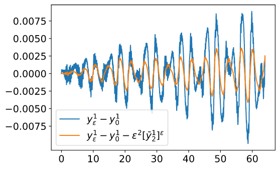
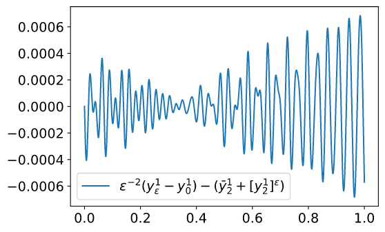
Finally, we analyse the viability of the second-order asymptotic expansion as a suitable approximation to the slow degrees of freedom of system (1) from a numerical point of view. More precisely, we choose a specific model from the class of fast–slow Hamiltonian systems represented by (1) and compare the numerical solution of yεy_{\varepsilon} with y0+ε2​(y¯2+[y2]ε)y_{0}+\varepsilon^{2}(\bar{y}_{2}+[y_{2}]^{\varepsilon}) in terms of its short- and long-term approximation quality and computation time. The maximal time frame for which an approximation of yεy_{\varepsilon} can be considered sufficiently accurate significantly increases by using y0+ε2​(y¯2+[y2]ε)y_{0}+\varepsilon^{2}(\bar{y}_{2}+[y_{2}]^{\varepsilon}) instead of y0y_{0} alone. Moreover, we show that the computation of y0+ε2​(y¯2+[y2]ε)y_{0}+\varepsilon^{2}(\bar{y}_{2}+[y_{2}]^{\varepsilon}) is up to two orders of magnitude faster (depending on the scale parameter ε\varepsilon) than a computation of yεy_{\varepsilon} to comparable accuracy as a solution to system (1). As described earlier, the reason is that fast oscillations severely affect the runtime for numerically computing yεy_{\varepsilon} from (1). In contrast, the problematic oscillatory term at second-order [y2]ε[y_{2}]^{\varepsilon} is given explicitly, and the derivation of y0y_{0} and y¯2\bar{y}_{2} only require a numerical integration of two slow systems of differential equations, which can be solved, in parallel, using a relatively large step size.

An application of the theory presented in this article may not only improve large-scale molecular dynamics simulations. It can also find applications in cases where the homogenisation theory outlined above and related work as in [22] are applicable. Some examples are given by the description of quantum–classical models in quantum-chemistry [3], the problem of deriving the guiding centre motion in plasma physics [4] or, more recently, the derivation of a coarse-grained description of the coupled thermoelastic behaviour from an atomistic model in materials science [17].

Finally, we want to point out other thermodynamic analyses based on the fast–slow system governed by the Lagrangian (1). In [13], the authors extend system (1) by coupling the fast and slow degrees of freedom to an external Nosé–Hoover thermostat and analyse the thermodynamic equilibration of the system on the fast and slow scale. In a similar line of thought, the authors in [23] expand system (1) by embedding it into an external heat bath and subsequently analysing the resulting slow dynamics, analogous to the homogenisation procedure introduced above, in the limit ε→0\varepsilon\to 0.

1.1 Outline of the paper

In Section 2 we introduce the model problem, which establishes the foundation for the analysis in this article, and state necessary non-resonance conditions, which ensure that the subsequently derived second-order expansion of the solution to the model problem is well-defined. A summary of our main results is provided in Section 3. We start the analysis of the model problem by introducing a transformation of the fast degrees of freedom into action–angle variables in Section 4, where we also prove the existence and uniqueness of a solution of the transformed system. In Section 5 we introduce some notation that simplifies the governing equations of motion and derive the second-order asymptotic expansion for the transformed degrees of freedom. Subsequently, in Section 6, we define expressions for the temperature, the entropy and the external force for the fast subsystem and interpret the model from a thermodynamic point of view. For a test model, the global error for approximating yεy_{\varepsilon} by y0+ε2​(y¯2+[y2]ε)y_{0}+\varepsilon^{2}(\bar{y}_{2}+[y_{2}]^{\varepsilon}) are analysed on short and long time intervals in Section 7, where we also compare the runtimes for computing yεy_{\varepsilon}, y0y_{0} and y¯2+[y2]ε\bar{y}_{2}+[y_{2}]^{\varepsilon}. Section 8 provides a short conclusion of this article. In Appendix A we summarise how the thermodynamic expressions can be derived for the fast subsystem. Finally, in Appendix B we present some data on the computation times corresponding to the maximal step sizes used in the numerical simulations presented in this article.

2 The model problem

For a small scale parameter 0<ε<ε0<∞0<\varepsilon<\varepsilon_{0}<\infty, we study the family of mechanical systems given by the Lagrangian

(3) ℒε​(x,x˙)=12​⟨x˙,x˙⟩−Wε​(x),x˙∈Tx​M,\mathscr{L}_{\varepsilon}(x,\dot{x})=\tfrac{1}{2}\left\langle\dot{x},\dot{x}\right\rangle-W_{\varepsilon}(x),\qquad\dot{x}\in T_{x}M,

on a Euclidean configuration space M=ℝmM=\mathbb{R}^{m}. Here and in the following, ⟨⋅,⋅⟩\left\langle\cdot,\cdot\right\rangle denotes Euclidean inner products and |⋅|\left|\cdot\right| denotes Euclidean norms. Splitting the coordinates according to x=(y,z)∈ℝn×ℝr=ℝmx=(y,z)\in\mathbb{R}^{n}\times\mathbb{R}^{r}=\mathbb{R}^{m}, we specify, following [3], the potential Wε=V+ε−2​UW_{\varepsilon}=V+\varepsilon^{-2}U by a smooth potential V=V⁡(y)V=V(y), which is assumed to be bounded from below and

(4) U⁡(x)=12​⟨H⁡(y)​z,z⟩withH⁡(y)=diag⁡(ω12​(y),…,ωr2​(y)).U(x)=\tfrac{1}{2}\left\langle H(y)z,z\right\rangle\qquad\text{with}\qquad H(y)=\mathrm{diag}(\omega_{1}^{2}(y),\ldots,\omega_{r}^{2}(y)).

We assume that the smooth functions ωλ∈C∞​(ℝn)\omega_{\lambda}\in C^{\infty}(\mathbb{R}^{n}) are uniformly positive, i.e., there exists a constant ω∗>0\omega_{\ast}>0 such that

(5) ωλ(y)≥ω∗,y∈ℝn,λ=1,…,r.\omega_{\lambda}(y)\geq\omega_{\ast},\qquad y\in\mathbb{R}^{n},\quad\lambda=1,\ldots,r.

A componentwise formulation of the equations of motion for the ε\varepsilon-dependent coordinates yεy_{\varepsilon} and zεz_{\varepsilon} in (3) yields

(6a) y¨εj\displaystyle\ddot{y}_{\varepsilon}^{j} =\displaystyle= −∂jV(yε)−12ε−2⟨∂jH(yε)zε,zε⟩,j=1,…,n,\displaystyle-\partial_{j}V(y_{\varepsilon})-\tfrac{1}{2}\varepsilon^{-2}\left\langle\partial_{j}H(y_{\varepsilon})z_{\varepsilon},z_{\varepsilon}\right\rangle,\qquad j=1,\ldots,n,
(6b) z¨ε\displaystyle\ddot{z}_{\varepsilon} =\displaystyle= −ε−2​H​(yε)​zε.\displaystyle-\varepsilon^{-2}H(y_{\varepsilon})z_{\varepsilon}.

Moreover, we consider the ε\varepsilon-independent initial values

(7) yε​(0)=y∗,y˙ε​(0)=p∗,zε​(0)=0,z˙ε​(0)=u∗.y_{\varepsilon}(0)=y_{\ast},\qquad\dot{y}_{\varepsilon}(0)=p_{\ast},\qquad z_{\varepsilon}(0)=0,\qquad\dot{z}_{\varepsilon}(0)=u_{\ast}.

We notice that the energy EεE_{\varepsilon} of the system is independent of ε\varepsilon due to the particular choice zε​(0)=0z_{\varepsilon}(0)=0,

(8) Eε=12​|y˙ε|2+12​|z˙ε|2+V⁡(yε)+ε−2​U​(yε,zε)=12​|p∗|2+12​|u∗|2+V⁡(y∗)=E∗.E_{\varepsilon}=\tfrac{1}{2}\left|\dot{y}_{\varepsilon}\right|^{2}+\tfrac{1}{2}\left|\dot{z}_{\varepsilon}\right|^{2}+V(y_{\varepsilon})+\varepsilon^{-2}U(y_{\varepsilon},z_{\varepsilon})=\tfrac{1}{2}\left|p_{\ast}\right|^{2}+\tfrac{1}{2}\left|u_{\ast}\right|^{2}+V(y_{\ast})=E_{\ast}.
Remark.

For the equations in (6a)–(8) and below, we will simultaneously make use of the vector notation for the coordinates yε∈ℝny_{\varepsilon}\in\mathbb{R}^{n} and zε∈ℝrz_{\varepsilon}\in\mathbb{R}^{r} (and related expressions) as well as their componentwise representation yεjy_{\varepsilon}^{j} (j=1,…,n)(j=1,\ldots,n) and zελz_{\varepsilon}^{\lambda} (λ=1,…,r)(\lambda=1,\ldots,r). The index in the superscript should not be confused with an exponent.

We are primarily interested in the evolution of the slow degrees of freedom yεjy_{\varepsilon}^{j} (j=1,…,n)(j=1,\ldots,n). The following theorem by Bornemann shows that yεy_{\varepsilon} converges in the limit ε→0\varepsilon\to 0 to a function y0y_{0} which is given as the solution to a second-order differential equation.

Theorem 2.1 (Bornemann, [3]).

For

Uhom​(y0)=∑λ=1rθ∗λ​ωλ​(y0),whereθ∗λ=|u∗λ|22​ωλ​(y∗),λ=1,…,r,U_{\hom}(y_{0})=\sum_{\lambda=1}^{r}\theta_{\ast}^{\lambda}\omega_{\lambda}(y_{0}),\qquad\text{where}\qquad\theta_{\ast}^{\lambda}=\frac{\left|u_{\ast}^{\lambda}\right|^{2}}{2\omega_{\lambda}(y_{\ast})},\qquad\lambda=1,\ldots,r,

let y0y_{0} be the solution to the second-order differential equation

(9) y¨0j=−∂jV(y0)−∂jUhom(y0),j=1,…,n,\ddot{y}_{0}^{j}=-\partial_{j}V(y_{0})-\partial_{j}U_{\hom}(y_{0}),\qquad j=1,\ldots,n,

with initial values y0​(0)=y∗y_{0}(0)=y_{\ast}, y˙0​(0)=p∗\dot{y}_{0}(0)=p_{\ast}. Then, for every finite time interval [0,T][0,T], we obtain the strong convergence

yε→y0inC1​([0,T],ℝn)y_{\varepsilon}\to y_{0}\quad\text{in}\quad C^{1}([0,T],\mathbb{R}^{n})

and the weak∗ convergences ε−1​zε⇀∗0\varepsilon^{-1}z_{\varepsilon}\stackrel{{\scriptstyle\ast}}{{\rightharpoonup}}0 and z˙ε⇀∗0\dot{z}_{\varepsilon}\stackrel{{\scriptstyle\ast}}{{\rightharpoonup}}0 in L∞​([0,T],ℝr)L^{\infty}([0,T],\mathbb{R}^{r}).

Theorem 2.1 shows that the family of mechanical systems (3) converges as ε→0\varepsilon\to 0 to a mechanical system which is again Hamiltonian.

2.1 Non-resonance conditions

As the interaction of multiple oscillating degrees of freedom can lead to resonance effects in the system, we will, similar to [3], impose suitable non-resonance conditions on the frequencies ωλ\omega_{\lambda} to ensure that the second-order asymptotic expansions, which we will derive in Section 5, are well-defined. We say, referring to the definition stated for example in [31, Section 14.6], that a resonance of order j∈ℕj\in\mathbb{N} at y∈ℝny\in\mathbb{R}^{n} is given by the relation

(10) γ1​ω1​(y)+⋯+γr​ωr​(y)=0,|γ1|+⋯+|γr|=j,\gamma_{1}\omega_{1}(y)+\cdots+\gamma_{r}\omega_{r}(y)=0,\qquad\left|\gamma_{1}\right|+\cdots+\left|\gamma_{r}\right|=j,

with integer coefficients γλ∈ℤ\gamma_{\lambda}\in\mathbb{Z} for λ=1,…,r\lambda=1,\ldots,r. Note that the non-degeneracy condition (5) implies that there is no resonance of order one.

Assumption 1.

We assume that the homogenised solution in Theorem 2.1 is non-resonant of order two, i.e., we assume that

γ1​ω1​(y0​(t))+⋯+γr​ωr​(y0​(t))≠0,|γ1|+⋯+|γr|=2,\gamma_{1}\omega_{1}(y_{0}(t))+\cdots+\gamma_{r}\omega_{r}(y_{0}(t))\neq 0,\qquad\left|\gamma_{1}\right|+\cdots+\left|\gamma_{r}\right|=2,

for all t∈[0,T]t\in[0,T].

Assumption 2.

Moreover, we assume that the homogenised solution in Theorem 2.1 is not flatly resonant up to order three. More precisely, we assume that

dd​t​(γ1​ω1​(y0​(ti))+⋯+γr​ωr​(y0​(ti)))≠0,|γ1|+⋯+|γr|≤3,\frac{d}{dt}\left(\gamma_{1}\omega_{1}(y_{0}(t_{i}))+\cdots+\gamma_{r}\omega_{r}(y_{0}(t_{i}))\right)\neq 0,\qquad\left|\gamma_{1}\right|+\cdots+\left|\gamma_{r}\right|\leq 3,

for all impact times ti∈[0,T]t_{i}\in[0,T] (i∈I⊂ℕ,I finite)(i\in I\subset\mathbb{N},I\text{ finite}) such that the non-resonance condition (10) holds at y0​(ti)y_{0}(t_{i}).

We remark that Assumption 1 is intentionally chosen to simplify the derivation of the second-order asymptotic expansions (see remark following Lemma 5.9). Under these simplifications the assumption also ensures, that the second-order asymptotic expansions derived in Section 5 are well-defined. Assumption 2 is, analogous to [3], a necessary prerequisite for the theory developed below. It ensures that rapidly oscillating functions of the form exp⁡(±i​ε−1​(ωλ​(yε)−ωμ​(yε)))\exp\left(\pm i\varepsilon^{-1}\left(\omega_{\lambda}(y_{\varepsilon})-\omega_{\mu}(y_{\varepsilon})\right)\right) and exp⁡(±i​ε−1​(ωλ​(yε)+ων​(yε)−ωμ​(yε)))\exp\left(\pm i\varepsilon^{-1}\left(\omega_{\lambda}(y_{\varepsilon})+\omega_{\nu}(y_{\varepsilon})-\omega_{\mu}(y_{\varepsilon})\right)\right) where λ,μ,ν=1,…,r\lambda,\mu,\nu=1,\ldots,r, λ≠μ\lambda\neq\mu converge weakly∗ to zero in L∞​([0,T])L^{\infty}([0,T]). In [3] these functions appear due to interactions of the fast degrees of freedom caused by the structure of a more general potential U⁡(x)U(x) as well as a more general metric ⟨⋅,⋅⟩\left\langle\cdot,\cdot\right\rangle and Assumption 2 is used to derive the leading-order asymptotic expansion of the system’s degrees of freedom. Here, however, these functions appear only due to small-scale interactions in the second-order asymptotic expansions.

3 Summary of the main results

The goal of this article is to extend the theory developed in [3] by deriving the second-order asymptotic expansion rigorously for the solution of the equations of motion (6a) and interpret the corresponding second-order asymptotic expansion of the energy (8) from a thermodynamic point of view. Note that the mechanical system (3) is not a classical thermodynamic system. In particular, the fast subsystem, consisting of the fast degrees of freedom zελz_{\varepsilon}^{\lambda} (λ=1,…,r)(\lambda=1,\ldots,r), which we will consider in Section 6 as the thermodynamic part of the whole system, is in general not ergodic. Finally, we will discuss the numerical implications of the second-order asymptotic expansion of yεy_{\varepsilon} in terms of its approximation error and computational cost.

Our main findings in this article can be summarised as follows.

  1. 1.

    After transforming the rapidly oscillating degrees of freedom into action–angle variables (zε,z˙ε)↦(θε,ϕε)(z_{\varepsilon},\dot{z}_{\varepsilon})\mapsto(\theta_{\varepsilon},\phi_{\varepsilon}), which also involves a transformation of the generalised momentum y˙ε↦pε\dot{y}_{\varepsilon}\mapsto p_{\varepsilon}, we derive the second-order asymptotic expansion of yε,pε,θε,ϕεy_{\varepsilon},p_{\varepsilon},\theta_{\varepsilon},\phi_{\varepsilon}. This takes the form

    yε\displaystyle y_{\varepsilon} =\displaystyle= y0\displaystyle y_{0} + ε[ ¯ y _1]^ε + ε^2[ ¯ y _2]^ε + ε^2y_3^ε,
    pε\displaystyle p_{\varepsilon} =\displaystyle= p0\displaystyle p_{0} + ε[ ¯ p _1]^ε + ε^2[ ¯ p _2]^ε + ε^2p_3^ε,
    θε\displaystyle\theta_{\varepsilon} =\displaystyle= θ∗\displaystyle\theta_{\ast} + ε[ ¯ θ _1]^ε + ε^2[ ¯ θ _2]^ε + ε^2θ_3^ε,
    ϕε\displaystyle\phi_{\varepsilon} =\displaystyle= ϕ0\displaystyle\phi_{0} + ε[ ¯ ϕ _1]^ε + ε^2[ ¯ ϕ _2]^ε + ε^2ϕ_3^ε,

    where for i∈{1,2}i\in\{1,2\},

    [y¯i]ε\displaystyle[\bar{y}_{i}]^{\varepsilon} ≔\displaystyle\coloneqq y¯i\displaystyle\bar{y}_{i} + [y_i]^ε ⇀ ∗ ¯ y _i in  L^∞([0,T], R^n), y_3^ε → 0 in  C([0,T], R^n),
    [p¯i]ε\displaystyle\phantom{}[\bar{p}_{i}]^{\varepsilon} ≔\displaystyle\coloneqq p¯i\displaystyle\bar{p}_{i} + [p_i]^ε ⇀ ∗ ¯ p _i in  L^∞([0,T], R^n), p_3^ε → 0 in  C([0,T], R^n),
    [θ¯i]ε\displaystyle\phantom{}[\bar{\theta}_{i}]^{\varepsilon} ≔\displaystyle\coloneqq θ¯i\displaystyle\bar{\theta}_{i} + [θ_i]^ε ⇀ ∗ ¯ θ _i in  L^∞([0,T],R^r), θ_3^ε → 0 in  C([0,T],R^r),
    [ϕ¯i]ε\displaystyle\phantom{}[\bar{\phi}_{i}]^{\varepsilon} ≔\displaystyle\coloneqq ϕ¯i\displaystyle\bar{\phi}_{i} + [ϕ_i]^ε ⇀ ∗ ¯ ϕ _i in  L^∞([0,T],R^r), ϕ_3^ε → 0 in  C([0,T],R^r).

    In other words, for each degree of freedom the second-order asymptotic expansion is characterised – to leading-order by the theory developed in [3] (Theorem 2.1) – to iith order by a decomposition into a slow term, indicated by an overbar, which constitutes the average motion of the iith order expansion, and a fast term, indicated by square brackets, which oscillates rapidly and converges weakly∗ to zero — and by a residual term, indicated with a subscript three, which converges uniformly to zero. In particular, we show that

    [y¯1]ε=0,[p¯1]ε=0,[θ¯1]ε=[θ1]ε,[ϕ¯1]ε=0,[\bar{y}_{1}]^{\varepsilon}=0,\qquad[\bar{p}_{1}]^{\varepsilon}=0,\qquad[\bar{\theta}_{1}]^{\varepsilon}=[\theta_{1}]^{\varepsilon},\qquad[\bar{\phi}_{1}]^{\varepsilon}=0,

    and that (ϕ¯2,θ¯2,y¯2,p¯2)(\bar{\phi}_{2},\bar{\theta}_{2},\bar{y}_{2},\bar{p}_{2}) is given as the solution to an inhomogeneous linear system of differential equations (Theorem 5.2). Moreover, the rapidly oscillating functions [θ1]ε[\theta_{1}]^{\varepsilon}, [y2]ε[y_{2}]^{\varepsilon}, [p2]ε[p_{2}]^{\varepsilon}, [θ2]ε[\theta_{2}]^{\varepsilon} and [ϕ2]ε[\phi_{2}]^{\varepsilon} are explicitly given in Definition 5.1.

  2. 2.

    In [11], Hertz formalises a thermodynamic theory for fast Hamiltonian systems which are perturbed by slow external agents. We regard the fast subsystem (zε,z˙ε)(z_{\varepsilon},\dot{z}_{\varepsilon}) as such a thermodynamic system, perturbed by the slow motion of (yε,y˙ε)(y_{\varepsilon},\dot{y}_{\varepsilon}). Since the fast subsystem is not ergodic, we follow along the lines of [2, Chapter 1.10] and replace the time average, which is an essential component in the thermodynamic theory, by the ensemble average, i.e., the average over uniformly distributed initial values on the energy surface (see Appendix A), and define, based on Hertz’ formulation, a temperature TεT_{\varepsilon}, an entropy SεS_{\varepsilon} and an external force FεF_{\varepsilon} for the fast subsystem.

    In combination with the analytic result discussed under 1, we decompose the total energy EεE_{\varepsilon} into the energy associated with the fast subsystem Eε⟂E_{\varepsilon}^{\perp} and its residual energy Eε∥=Eε−Eε⟂E_{\varepsilon}^{\parallel}=E_{\varepsilon}-E_{\varepsilon}^{\perp}, and expand, similar to above Eε⟂E_{\varepsilon}^{\perp}, Eε∥E_{\varepsilon}^{\parallel}, TεT_{\varepsilon}, SεS_{\varepsilon} and FεF_{\varepsilon} into the form

    Eε⟂\displaystyle E_{\varepsilon}^{\perp} =\displaystyle= E0⟂\displaystyle E_{0}^{\perp} + ε[ ¯ E _1^⟂]^ε + ε^2[ ¯ E _2^⟂]^ε + ε^2E_3^⟂ε,
    Eε∥\displaystyle E_{\varepsilon}^{\parallel} =\displaystyle= E0∥\displaystyle E_{0}^{\parallel} + ε[ ¯ E _1^∥]^ε + ε^2[ ¯ E _2^∥]^ε + ε^2E_3^∥ε,
    Sε\displaystyle S_{\varepsilon} =\displaystyle= S0\displaystyle S_{0} + ε[ ¯ S _1]^ε + ε^2[ ¯ S _2]^ε + ε^2S_3^ε,
    Tε\displaystyle T_{\varepsilon} =\displaystyle= T0\displaystyle T_{0} + O(ε),
    Fε\displaystyle F_{\varepsilon} =\displaystyle= F0\displaystyle F_{0} + O(ε),

    where for i∈{1,2}i\in\{1,2\},

    [E¯i⟂]ε\displaystyle[\bar{E}_{i}^{\perp}]^{\varepsilon} ≔\displaystyle\coloneqq E¯i⟂\displaystyle\bar{E}_{i}^{\perp} + [E_i^⟂]^ε ⇀ ∗ ¯ E _i^⟂ in  L^∞([0,T]), E_3^⟂ε → 0 in  C([0,T]),
    [E¯i∥]ε\displaystyle\phantom{}[\bar{E}_{i}^{\parallel}]^{\varepsilon} ≔\displaystyle\coloneqq E¯i∥\displaystyle\bar{E}_{i}^{\parallel} + [E_i^∥]^ε ⇀ ∗ ¯ E _i^∥ in  L^∞([0,T]), E_3^∥ε → 0 in  C([0,T]),
    [S¯i]ε\displaystyle\phantom{}[\bar{S}_{i}]^{\varepsilon} ≔\displaystyle\coloneqq S¯i\displaystyle\bar{S}_{i} + [S_i]^ε ⇀ ∗ ¯ S _i in  L^∞([0,T]), S_3^ε → 0 in  C([0,T]).

    The characterisation of the iith order expansion is similar to 1 and is already discussed, for the case of n=r=1n=r=1, in [14]. In Section 6 we interpret these asymptotic expansions from a thermodynamic point of view. In particular, we show that, to leading-order, the dynamics can be interpreted as a thermodynamic process characterised by the energy relation

    d​E0⟂=∑j=1nF0j​d​y0j+T0​d​S0.dE_{0}^{\perp}=\sum_{j=1}^{n}F_{0}^{j}dy^{j}_{0}+T_{0}dS_{0}.

    In contrast to the analysis in [14], we find, provided that θ∗λ≠0\theta_{\ast}^{\lambda}\neq 0 for at least one λ=1,…,r\lambda=1,\ldots,r, that the entropy expression to leading-order is constant, d​S0=0dS_{0}=0, if and only if all pairwise weighted frequency ratios θ∗λ​ωλ​(y0)/ωμ​(y0)\theta_{\ast}^{\lambda}\omega_{\lambda}(y_{0})/\omega_{\mu}(y_{0}) (λ,μ=1,…,r)(\lambda,\mu=1,\ldots,r) are constant. In this case, the leading-order dynamics can be interpreted as an adiabatic thermodynamic process. Yet, if any of the weighted frequency ratios is non-constant, the entropy is non-constant and thus the leading-order dynamics can be interpreted as a non-adiabatic thermodynamic process. Here we use the definition of entropy given by Hertz in a context where the entropy is not necessarily the logarithm of an adiabatic invariant. Nevertheless, we show that a meaningful thermodynamic interpretation can be given.

    Furthermore, we show that the averaged second-order dynamics, i.e., the dynamics in the weak∗ limit of the second-order terms, indicated by an overbar, represents for fixed (y0,p0)(y_{0},p_{0}) a non-adiabatic thermodynamic process with an averaged non-constant entropy, d​S¯2≠0d\bar{S}_{2}\neq 0, which also satisfies relations akin to equilibrium thermodynamics, despite being beyond the limit ε→0\varepsilon\to 0,

    d​E¯2⟂=∑j=1nF0j​d​y¯2j+T0​d​S¯2.d\bar{E}_{2}^{\perp}=\sum_{j=1}^{n}F_{0}^{j}d\bar{y}_{2}^{j}+T_{0}d\bar{S}_{2}.

    Finally, we show in Theorem 6.1 that the evolution of (y¯2,p¯2)(\bar{y}_{2},\bar{p}_{2}) is governed by equations which resemble Hamilton’s canonical equations,

    d​y¯2d​t=∂E¯2∂p0,∂p¯2d​t=−∂E¯2∂y0,\frac{d\bar{y}_{2}}{dt}=\frac{\partial\bar{E}_{2}}{\partial p_{0}},\qquad\frac{\partial\bar{p}_{2}}{dt}=-\frac{\partial\bar{E}_{2}}{\partial y_{0}},

    for E¯2=E¯2⟂+E¯2∥\bar{E}_{2}=\bar{E}_{2}^{\perp}+\bar{E}_{2}^{\parallel}, which are complemented by the ε\varepsilon-independent initial values

    y¯2​(0)=−[y2]ε​(0),p¯2​(0)=−[p2]ε​(0).\bar{y}_{2}(0)=-[y_{2}]^{\varepsilon}(0),\qquad\bar{p}_{2}(0)=-[p_{2}]^{\varepsilon}(0).
  3. 3.

    Finally, we compare in numerical simulations the second-order asymptotic expansion of the slow degrees of freedom y0+ε2​(y¯2+[y2]ε)y_{0}+\varepsilon^{2}(\bar{y}_{2}+[y_{2}]^{\varepsilon}) with simulations for yεy_{\varepsilon} of the original system (6a). The latter is computationally expensive, as it requires a numerical integration of the fast degrees of freedom zεz_{\varepsilon}. To this end, we derive numerically the slow motion y0y_{0} of the leading-order system (9) and the average motion y¯2\bar{y}_{2} of the second-order system (23a) and combine them with the explicitly given rapidly oscillating components [y2]ε[y_{2}]^{\varepsilon} of the second-order expansion as specified in Definition 5.1. We find, depending on the value of the scale parameter ε\varepsilon, that the computation time for the second-order expansion is up to two orders of magnitude faster than the computation time for the slow degrees of freedom of the original system. Moreover, we show that y0+ε2​(y¯2+[y2]ε)y_{0}+\varepsilon^{2}(\bar{y}_{2}+[y_{2}]^{\varepsilon}) provides an approximation of yεy_{\varepsilon} which has significantly better global error bounds on long time intervals than an approximation by y0y_{0} alone.

4 The model problem in action–angle variables

To study the dynamics of yεy_{\varepsilon} and zεz_{\varepsilon} on different scales, a detailed asymptotic analysis is required. Such an analysis was already presented for the model problem as introduced in Section 2 in the case of one fast and one slow degree of freedom (i.e., n=r=1n=r=1) in [14], which extends the analysis given in [3, Appendix C]. To derive the second-order asymptotic expansion of the solution to the model problem for arbitrary n,r∈ℕn,r\in\mathbb{N}, we analogously start by rephrasing the governing system of Newtonian equations (6a) by transforming the fast degrees of freedom (zε,z˙ε)(z_{\varepsilon},\dot{z}_{\varepsilon}) into action–angle variables (θε,ϕε)(\theta_{\varepsilon},\phi_{\varepsilon}).

We denote the canonical momenta corresponding to the positions (yε,zε)(y_{\varepsilon},z_{\varepsilon}) as (ηε,ζε)(\eta_{\varepsilon},\zeta_{\varepsilon}). Then, the equations of motion (6a), together with the velocity relations

y˙ε=ηε,z˙ε=ζε,\dot{y}_{\varepsilon}=\eta_{\varepsilon},\qquad\dot{z}_{\varepsilon}=\zeta_{\varepsilon},

are given by the canonical equations of motion belonging to the energy function

Eε=12​|ηε|2+12​|ζε|2+V⁡(yε)+12​ε−2​∑λ=1rωλ2​(yε)​(zελ)2.E_{\varepsilon}=\frac{1}{2}|\eta_{\varepsilon}|^{2}+\frac{1}{2}|\zeta_{\varepsilon}|^{2}+V(y_{\varepsilon})+\frac{1}{2}\varepsilon^{-2}\sum_{\lambda=1}^{r}\omega_{\lambda}^{2}(y_{\varepsilon})(z_{\varepsilon}^{\lambda})^{2}.

The transformation (zε,ζε)↦(θε,ϕε)(z_{\varepsilon},\zeta_{\varepsilon})\mapsto(\theta_{\varepsilon},\phi_{\varepsilon}) can be found by the theory of generating functions [1] as presented in [3, Appendix C]. For fixed yεy_{\varepsilon}, the generating function is given by

S0​(zε,ϕε,yε)=12​ε​∑λ=1rωλ​(yε)​(zελ)2​cot⁡(ε−1​ϕελ),S_{0}(z_{\varepsilon},\phi_{\varepsilon};y_{\varepsilon})=\frac{1}{2\varepsilon}\sum_{\lambda=1}^{r}\omega_{\lambda}(y_{\varepsilon})(z_{\varepsilon}^{\lambda})^{2}\cot(\varepsilon^{-1}\phi_{\varepsilon}^{\lambda}),

via ζε=∂S0/∂zε\zeta_{\varepsilon}=\partial S_{0}/\partial z_{\varepsilon} and θε=−∂S0/∂ϕε\theta_{\varepsilon}=-\partial S_{0}/\partial\phi_{\varepsilon}. With this transformation, the fast degrees of freedom (zε,ζε)(z_{\varepsilon},\zeta_{\varepsilon}) can be written as

zελ=ε​2​θελωλ​(yε)​sin⁡(ε−1​ϕελ),ζελ=2​θελ​ωλ​(yε)​cos⁡(ε−1​ϕελ).z_{\varepsilon}^{\lambda}=\varepsilon\sqrt{\frac{2\theta_{\varepsilon}^{\lambda}}{\omega_{\lambda}(y_{\varepsilon})}}\sin(\varepsilon^{-1}\phi_{\varepsilon}^{\lambda}),\qquad\zeta_{\varepsilon}^{\lambda}=\sqrt{2\theta_{\varepsilon}^{\lambda}\omega_{\lambda}(y_{\varepsilon})}\cos(\varepsilon^{-1}\phi_{\varepsilon}^{\lambda}).

It turns out, however, that the transformation (zε,ζε)↦(θε,ϕε)(z_{\varepsilon},\zeta_{\varepsilon})\mapsto(\theta_{\varepsilon},\phi_{\varepsilon}) is symplectic only for fixed yεy_{\varepsilon}. To derive a transformation that preserves the symplectic structure on the whole phase-space, one introduces the generalised momenta pεp_{\varepsilon} through another transformation ηε↦pε\eta_{\varepsilon}\mapsto p_{\varepsilon}. To this end, we define the extended generating function S⁡(yε,pε,zε,ϕε)=pεT​yε+S0​(zε,ϕε,yε)S(y_{\varepsilon},p_{\varepsilon},z_{\varepsilon},\phi_{\varepsilon})=p_{\varepsilon}^{T}y_{\varepsilon}+S_{0}(z_{\varepsilon},\phi_{\varepsilon};y_{\varepsilon}) which does not transform the position yε=∂S/∂pεy_{\varepsilon}=\partial S/\partial p_{\varepsilon}, but changes the momentum ηε\eta_{\varepsilon} such that the transformation remains symplectic on the whole phase-space. The missing transformation of the momentum ηε\eta_{\varepsilon} is given componentwise for j=1,…,nj=1,\ldots,n by

ηεj=∂S∂yεj=pεj+ε​∑λ=1rθελ⋅∂jωλ​(yε)2​ωλ​(yε)​sin⁡(2​ε−1​ϕελ).\eta_{\varepsilon}^{j}=\frac{\partial S}{\partial y^{j}_{\varepsilon}}=p^{j}_{\varepsilon}+\varepsilon\sum_{\lambda=1}^{r}\frac{\theta_{\varepsilon}^{\lambda}\cdot\partial_{j}\omega_{\lambda}(y_{\varepsilon})}{2\omega_{\lambda}(y_{\varepsilon})}\sin(2\varepsilon^{-1}\phi^{\lambda}_{\varepsilon}).

By construction, the resulting transformation (yε,ηε,zε,ζε)↦(yε,pε,ϕε,θε)(y_{\varepsilon},\eta_{\varepsilon};z_{\varepsilon},\zeta_{\varepsilon})\mapsto(y_{\varepsilon},p_{\varepsilon};\phi_{\varepsilon},\theta_{\varepsilon}) is symplectic.

The energy can be expressed in the new coordinates as

Eε\displaystyle E_{\varepsilon} =\displaystyle= 12​|pε|2+V⁡(yε)+∑λ=1rθελ​ωλ​(yε)+ε​∑j=1n∑λ=1rθελ​pεj⋅∂jωλ​(yε)2​ωλ​(yε)​sin⁡(2​ε−1​ϕελ)\displaystyle\frac{1}{2}|p_{\varepsilon}|^{2}+V(y_{\varepsilon})+\sum_{\lambda=1}^{r}\theta_{\varepsilon}^{\lambda}\omega_{\lambda}(y_{\varepsilon})+\varepsilon\sum_{j=1}^{n}\sum_{\lambda=1}^{r}\frac{\theta_{\varepsilon}^{\lambda}p_{\varepsilon}^{j}\cdot\partial_{j}\omega_{\lambda}(y_{\varepsilon})}{2\omega_{\lambda}(y_{\varepsilon})}\sin(2\varepsilon^{-1}\phi^{\lambda}_{\varepsilon})
+ε28∑j=1n(∑λ=1rθελ⋅∂jωλ​(yε)ωλ​(yε)sin(2ε−1ϕελ))2.\displaystyle+\>\frac{\varepsilon^{2}}{8}\sum_{j=1}^{n}\left(\sum_{\lambda=1}^{r}\frac{\theta_{\varepsilon}^{\lambda}\cdot\partial_{j}\omega_{\lambda}(y_{\varepsilon})}{\omega_{\lambda}(y_{\varepsilon})}\sin(2\varepsilon^{-1}\phi_{\varepsilon}^{\lambda})\right)^{2}.

Thus, by the canonical formalism, the equations of motion take the form

ϕ˙ελ=∂Eε∂θελ,θ˙ελ=−∂Eε∂ϕελ,y˙εj=∂Eε∂pεj,p˙εj=−∂Eε∂yεj,\dot{\phi}_{\varepsilon}^{\lambda}=\frac{\partial E_{\varepsilon}}{\partial\theta_{\varepsilon}^{\lambda}},\qquad\dot{\theta}_{\varepsilon}^{\lambda}=-\frac{\partial E_{\varepsilon}}{\partial\phi_{\varepsilon}^{\lambda}},\qquad\dot{y}_{\varepsilon}^{j}=\frac{\partial E_{\varepsilon}}{\partial p_{\varepsilon}^{j}},\qquad\dot{p}_{\varepsilon}^{j}=-\frac{\partial E_{\varepsilon}}{\partial y^{j}_{\varepsilon}},

for λ=1,…,r\lambda=1,\ldots,r and j=1,…,nj=1,\ldots,n. After some calculations, we find that these equations are given by

(11a) ϕ˙ελ\displaystyle\dot{\phi}^{\lambda}_{\varepsilon} =\displaystyle= ωλ​(yε)+ε​∑j=1npεj⋅∂jωλ​(yε)2​ωλ​(yε)​sin⁡(2​ε−1​ϕελ)\displaystyle\omega_{\lambda}(y_{\varepsilon})+\varepsilon\sum_{j=1}^{n}\frac{p^{j}_{\varepsilon}\cdot\partial_{j}\omega_{\lambda}(y_{\varepsilon})}{2\omega_{\lambda}(y_{\varepsilon})}\sin(2\varepsilon^{-1}\phi^{\lambda}_{\varepsilon})
(11b) +ε28∑j=1n∑μ=1rθεμ⋅∂jωμ​(yε)⋅∂jωλ​(yε)ωμ​(yε)​ωλ​(yε)(cos(2ε−1(ϕεμ−ϕελ))−cos(2ε−1(ϕεμ+ϕελ))),\displaystyle+\frac{\varepsilon^{2}}{8}\sum_{j=1}^{n}\sum_{\mu=1}^{r}\frac{\theta^{\mu}_{\varepsilon}\cdot\partial_{j}\omega_{\mu}(y_{\varepsilon})\cdot\partial_{j}\omega_{\lambda}(y_{\varepsilon})}{\omega_{\mu}(y_{\varepsilon})\omega_{\lambda}(y_{\varepsilon})}\left(\cos\left(2\varepsilon^{-1}\left(\phi_{\varepsilon}^{\mu}-\phi^{\lambda}_{\varepsilon}\right)\right)-\cos\left(2\varepsilon^{-1}\left(\phi_{\varepsilon}^{\mu}+\phi_{\varepsilon}^{\lambda}\right)\right)\right),
(11c) θ˙ελ\displaystyle\dot{\theta}^{\lambda}_{\varepsilon} =\displaystyle= −∑j=1nθελ​pεj⋅∂jωλ​(yε)ωλ​(yε)cos(2ε−1ϕελ)\displaystyle-\sum_{j=1}^{n}\frac{\theta^{\lambda}_{\varepsilon}p^{j}_{\varepsilon}\cdot\partial_{j}\omega_{\lambda}(y_{\varepsilon})}{\omega_{\lambda}(y_{\varepsilon})}\cos\left(2\varepsilon^{-1}\phi^{\lambda}_{\varepsilon}\right)
−ε4∑j=1n∑μ=1rθεμ​θελ⋅∂jωμ​(yε)⋅∂jωλ​(yε)ωμ​(yε)​ωλ​(yε)(sin(2ε−1(ϕεμ−ϕελ))+sin(2ε−1(ϕεμ+ϕελ))),\displaystyle-\frac{\varepsilon}{4}\sum_{j=1}^{n}\sum_{\mu=1}^{r}\frac{\theta^{\mu}_{\varepsilon}\theta^{\lambda}_{\varepsilon}\cdot\partial_{j}\omega_{\mu}(y_{\varepsilon})\cdot\partial_{j}\omega_{\lambda}(y_{\varepsilon})}{\omega_{\mu}(y_{\varepsilon})\omega_{\lambda}(y_{\varepsilon})}\left(\sin\left(2\varepsilon^{-1}\left(\phi_{\varepsilon}^{\mu}-\phi_{\varepsilon}^{\lambda}\right)\right)+\sin\left(2\varepsilon^{-1}\left(\phi_{\varepsilon}^{\mu}+\phi_{\varepsilon}^{\lambda}\right)\right)\right),
(11d) y˙εj\displaystyle\dot{y}^{j}_{\varepsilon} =\displaystyle= pεj+ε​∑λ=1rθελ⋅∂jωλ​(yε)2​ωλ​(yε)​sin⁡(2​ε−1​ϕελ),\displaystyle p^{j}_{\varepsilon}+\varepsilon\sum_{\lambda=1}^{r}\frac{\theta^{\lambda}_{\varepsilon}\cdot\partial_{j}\omega_{\lambda}(y_{\varepsilon})}{2\omega_{\lambda}(y_{\varepsilon})}\sin\left(2\varepsilon^{-1}\phi^{\lambda}_{\varepsilon}\right),
(11e) p˙εj\displaystyle\dot{p}^{j}_{\varepsilon} =\displaystyle= −∂jV(yε)−∑λ=1rθελ⋅∂jωλ(yε)−ε∑k=1n∑λ=1rθελ​pεk2(∂j∂kωλ​(yε)ωλ​(yε)−∂kωλ​(yε)⋅∂jωλ​(yε)ωλ2​(yε))sin(2ε−1ϕελ)\displaystyle-\partial_{j}V(y_{\varepsilon})-\sum_{\lambda=1}^{r}\theta^{\lambda}_{\varepsilon}\cdot\partial_{j}\omega_{\lambda}(y_{\varepsilon})-\varepsilon\sum_{k=1}^{n}\sum_{\lambda=1}^{r}\frac{\theta^{\lambda}_{\varepsilon}p^{k}_{\varepsilon}}{2}\left(\frac{\partial_{j}\partial_{k}\omega_{\lambda}(y_{\varepsilon})}{\omega_{\lambda}(y_{\varepsilon})}-\frac{\partial_{k}\omega_{\lambda}(y_{\varepsilon})\cdot\partial_{j}\omega_{\lambda}(y_{\varepsilon})}{\omega_{\lambda}^{2}(y_{\varepsilon})}\right)\sin\left(2\varepsilon^{-1}\phi^{\lambda}_{\varepsilon}\right)
−ε28∑k=1n∑λ=1r∑μ=1rθελ​θεμ⋅∂kωμ​(yε)ωμ​(yε)(∂j∂kωλ​(yε)ωλ​(yε)−∂kωλ​(yε)⋅∂jωλ​(yε)ωλ2​(yε))\displaystyle-\frac{\varepsilon^{2}}{8}\sum_{k=1}^{n}\sum_{\lambda=1}^{r}\sum_{\mu=1}^{r}\frac{\theta^{\lambda}_{\varepsilon}\theta^{\mu}_{\varepsilon}\cdot\partial_{k}\omega_{\mu}(y_{\varepsilon})}{\omega_{\mu}(y_{\varepsilon})}\left(\frac{\partial_{j}\partial_{k}\omega_{\lambda}(y_{\varepsilon})}{\omega_{\lambda}(y_{\varepsilon})}-\frac{\partial_{k}\omega_{\lambda}(y_{\varepsilon})\cdot\partial_{j}\omega_{\lambda}(y_{\varepsilon})}{\omega_{\lambda}^{2}(y_{\varepsilon})}\right)
×(cos⁡(2​ε−1​(ϕεμ−ϕελ))−cos⁡(2​ε−1​(ϕεμ+ϕελ))).\displaystyle\times\left(\cos\left(2\varepsilon^{-1}\left(\phi^{\mu}_{\varepsilon}-\phi^{\lambda}_{\varepsilon}\right)\right)-\cos\left(2\varepsilon^{-1}\left(\phi^{\mu}_{\varepsilon}+\phi^{\lambda}_{\varepsilon}\right)\right)\right).

The initial values as given in (7) transform to

(12) ϕε​(0)=0,θελ​(0)=θ∗λ=|u∗λ|22​ωλ​(y∗),yε​(0)=y∗,pε​(0)=p∗.\phi_{\varepsilon}(0)=0,\qquad\theta_{\varepsilon}^{\lambda}(0)=\theta_{\ast}^{\lambda}=\frac{|u_{\ast}^{\lambda}|^{2}}{2\omega_{\lambda}(y_{\ast})},\qquad y_{\varepsilon}(0)=y_{\ast},\qquad p_{\varepsilon}(0)=p_{\ast}.

4.1 Existence and uniqueness of a solution to the transformed model problem

Let us denote the right-hand side of (11a) as ℱε:ℝ2​m→ℝ2​m\mathcal{F}_{\varepsilon}\colon\mathbb{R}^{2m}\to\mathbb{R}^{2m}. By assumption ωλ∈C∞​(ℝn)\omega_{\lambda}\in C^{\infty}(\mathbb{R}^{n}) for λ=1,…,r\lambda=1,\ldots,r and therefore ℱε∈C∞​(ℝ2​m,ℝ2​m)\mathcal{F}_{\varepsilon}\in C^{\infty}(\mathbb{R}^{2m},\mathbb{R}^{2m}) for 0<ε<ε0<∞0<\varepsilon<\varepsilon_{0}<\infty. In particular, ℱε\mathcal{F}_{\varepsilon} is locally Lipschitz continuous. Hence, by the standard existence and uniqueness theory for ordinary differential equations (see for example [29]), there exists a T>0T>0 such that for fixed 0<ε<ε0<∞0<\varepsilon<\varepsilon_{0}<\infty the initial value problem (11a)–(12) has a unique solution

(13) (ϕε,θε,yε,pε)∈C∞​([0,T],ℝ2​m).(\phi_{\varepsilon},\theta_{\varepsilon},y_{\varepsilon},p_{\varepsilon})\in C^{\infty}([0,T],\mathbb{R}^{2m}).

5 Asymptotic expansion

In this section, we rigorously derive the second-order asymptotic expansion of ϕε\phi_{\varepsilon}, θε\theta_{\varepsilon}, yεy_{\varepsilon} and pεp_{\varepsilon}. We will see, that the leading-order expansion follows directly from the evolution equations (11a). To simplify these equations for the subsequent analysis, we introduce in Section 5.2 some suitable new notation. We then derive the first- and second-order asymptotic expansion in Section 5.3.

5.1 Leading-order expansion

We consider a sequence of solutions (13) for ε→0\varepsilon\to 0. The right-hand side of the evolution equations (11a) is oscillatory and has rapidly oscillating terms of leading-order. As a consequence, the sequences {ϕ˙ε}\{\dot{\phi}_{\varepsilon}\} and {θε}\{\theta_{\varepsilon}\} are bounded in C0,1​([0,T],ℝr)C^{0,1}([0,T],\mathbb{R}^{r}), and the sequences {y˙ε}\{\dot{y}_{\varepsilon}\} and {p˙ε}\{\dot{p}_{\varepsilon}\} are bounded in C0,1​([0,T],ℝn)C^{0,1}([0,T],\mathbb{R}^{n}), while sequences of higher-order derivatives (in particular {θ¨ε}\{\ddot{\theta}_{\varepsilon}\}, which will thus require special attention in the later part of this analysis) become unbounded as ε→0\varepsilon\to 0. It follows from the extended Arzelà–Ascoli theorem [3, Chapter I §1] that we can extract a subsequence, not relabelled, and functions θ0∈C0,1​([0,T],ℝr)\theta_{0}\in C^{0,1}([0,T],\mathbb{R}^{r}), ϕ0∈C1,1​([0,T],ℝr){\phi_{0}\in C^{1,1}([0,T],\mathbb{R}^{r})} and y0,p0∈C1,1​([0,T],ℝn)y_{0},p_{0}\in C^{1,1}([0,T],\mathbb{R}^{n}), such that

(14a) ϕε→ϕ0\displaystyle\phi_{\varepsilon}\to\phi_{0}  in C1​([0,T],ℝr),\displaystyle C^{1}([0,T],\mathbb{R}^{r}), ¨ ϕ _ε ⇀ ∗ ¨ ϕ _0  in L^∞([0,T],R^r),
(14b) θε→θ0\displaystyle\theta_{\varepsilon}\to\theta_{0}  in C⁡([0,T],ℝr),\displaystyle C([0,T],\mathbb{R}^{r}), ˙ θ _ε ⇀ ∗ ˙ θ _0  in L^∞([0,T],R^r),
(14c) yε→y0\displaystyle y_{\varepsilon}\to y_{0}  in C1​([0,T],ℝn),\displaystyle C^{1}([0,T],\mathbb{R}^{n}), ¨ y _ε ⇀ ∗ ¨ y _0  in L^∞([0,T],R^n),
(14d) pε→p0\displaystyle p_{\varepsilon}\to p_{0}  in C1​([0,T],ℝn),\displaystyle C^{1}([0,T],\mathbb{R}^{n}), ¨ p _ε ⇀ ∗ ¨ p _0  in L^∞([0,T],R^n).

By taking the limit ε→0\varepsilon\to 0 in Equations (11b), (11d) and (11e) and the weak∗ limit in (11c) we deduce that

ϕ˙0λ=ωλ(y0),θ˙0λ=0,y˙0j=p0j,p˙0j=−∂jV(y0)−∑λ=1rθ∗λ⋅∂jωλ(y0),\dot{\phi}^{\lambda}_{0}=\omega_{\lambda}(y_{0}),\qquad\dot{\theta}^{\lambda}_{0}=0,\qquad\dot{y}^{j}_{0}=p_{0}^{j},\qquad\dot{p}^{j}_{0}=-\partial_{j}V(y_{0})-\sum_{\lambda=1}^{r}\theta_{\ast}^{\lambda}\cdot\partial_{j}\omega_{\lambda}(y_{0}),

for λ=1,…,r\lambda=1,\ldots,r and j=1,…,nj=1,\ldots,n, and in particular that θ0λ≡θ∗λ\theta_{0}^{\lambda}\equiv\theta_{\ast}^{\lambda} (compare with (12)). Moreover, since the right-hand side of the limit equation

y¨0j=−∂jV(y0)−∑λ=1rθ∗λ⋅∂jωλ(y0)\ddot{y}^{j}_{0}=-\partial_{j}V(y_{0})-\sum_{\lambda=1}^{r}\theta_{\ast}^{\lambda}\cdot\partial_{j}\omega_{\lambda}(y_{0})

does not depend on a chosen subsequence, we can discard the extraction of a subsequence altogether (see [3, Principle 5, Chapter I §1]). Note that the above convergence results extend Theorem 2.1.

5.2 Reformulation of the governing equations

It will be convenient to introduce some notation to simplify the system of differential equations (11a). To this end, we define for f∈C∞​(ℝn)f\in C^{\infty}(\mathbb{R}^{n}), where f=f⁡(y)f=f(y) and y∈C∞​([0,T],ℝn)y\in C^{\infty}([0,T],\mathbb{R}^{n}), the expression

Dtk​Djl​f≔dkd​tk​∂lf∂yjl,D_{t}^{k}D_{j}^{l}f\coloneqq\frac{d^{k}}{dt^{k}}\frac{\partial^{l}f}{\partial y_{j}^{l}},

for k,l∈ℕ0k,l\in\mathbb{N}_{0} and j=1,…,nj=1,\ldots,n. We will often apply this notation in combination with the function

Lελ≔log⁡(ωλ​(yε)),L_{\varepsilon}^{\lambda}\coloneqq\log(\omega_{\lambda}(y_{\varepsilon})),

where λ=1,…,r\lambda=1,\ldots,r. Then, we can conveniently write, for instance,

(15) D​Lελ=∑j=1nDj​Lελ⋅ejorDt​Lελ=⟨y˙ε,D​Lελ⟩=∑j=1ny˙εj⋅Dj​Lελ,DL_{\varepsilon}^{\lambda}=\sum_{j=1}^{n}D_{j}L_{\varepsilon}^{\lambda}\cdot e_{j}\qquad\text{or}\qquad D_{t}L_{\varepsilon}^{\lambda}=\left\langle\dot{y}_{\varepsilon},DL_{\varepsilon}^{\lambda}\right\rangle=\sum_{j=1}^{n}\dot{y}_{\varepsilon}^{j}\cdot D_{j}L_{\varepsilon}^{\lambda},

with eje_{j} as the jjth standard basis vector in ℝn\mathbb{R}^{n}. With these definitions, the equations in (11a) read

(16a) ϕ˙ελ\displaystyle\dot{\phi}_{\varepsilon}^{\lambda} =\displaystyle= ωλ​(yε)+ε2​⟨pε,D​Lελ⟩​sin⁡(2​ε−1​ϕελ)\displaystyle\omega_{\lambda}(y_{\varepsilon})+\frac{\varepsilon}{2}\left\langle p_{\varepsilon},DL_{\varepsilon}^{\lambda}\right\rangle\sin(2\varepsilon^{-1}\phi_{\varepsilon}^{\lambda})
(16b) +ε28∑μ=1rθεμ⟨DLελ,DLεμ⟩(cos(2ε−1(ϕεμ−ϕελ))−cos(2ε−1(ϕεμ+ϕελ))),\displaystyle+\>\frac{\varepsilon^{2}}{8}\sum_{\mu=1}^{r}\theta_{\varepsilon}^{\mu}\left\langle DL_{\varepsilon}^{\lambda},DL_{\varepsilon}^{\mu}\right\rangle\left(\cos\left(2\varepsilon^{-1}\left(\phi_{\varepsilon}^{\mu}-\phi^{\lambda}_{\varepsilon}\right)\right)-\cos\left(2\varepsilon^{-1}\left(\phi_{\varepsilon}^{\mu}+\phi_{\varepsilon}^{\lambda}\right)\right)\right),
(16c) θ˙ελ\displaystyle\dot{\theta}_{\varepsilon}^{\lambda} =\displaystyle= −θελ​⟨pε,D​Lελ⟩​cos⁡(2​ε−1​ϕελ)\displaystyle-\theta_{\varepsilon}^{\lambda}\left\langle p_{\varepsilon},DL_{\varepsilon}^{\lambda}\right\rangle\cos(2\varepsilon^{-1}\phi_{\varepsilon}^{\lambda})
−ε4∑μ=1rθεμθελ⟨DLελ,DLεμ⟩(sin(2ε−1(ϕεμ−ϕελ))+sin(2ε−1(ϕεμ+ϕελ))),\displaystyle-\>\frac{\varepsilon}{4}\sum_{\mu=1}^{r}\theta_{\varepsilon}^{\mu}\theta_{\varepsilon}^{\lambda}\left\langle DL_{\varepsilon}^{\lambda},DL_{\varepsilon}^{\mu}\right\rangle\left(\sin\left(2\varepsilon^{-1}\left(\phi_{\varepsilon}^{\mu}-\phi_{\varepsilon}^{\lambda}\right)\right)+\sin\left(2\varepsilon^{-1}\left(\phi_{\varepsilon}^{\mu}+\phi_{\varepsilon}^{\lambda}\right)\right)\right),
(16d) y˙εj\displaystyle\dot{y}_{\varepsilon}^{j} =\displaystyle= pεj+ε2​∑λ=1nθελ⋅Dj​Lελ​sin⁡(2​ε−1​ϕελ),\displaystyle p_{\varepsilon}^{j}+\frac{\varepsilon}{2}\sum_{\lambda=1}^{n}\theta_{\varepsilon}^{\lambda}\cdot D_{j}L_{\varepsilon}^{\lambda}\sin(2\varepsilon^{-1}\phi_{\varepsilon}^{\lambda}),
(16e) p˙εj\displaystyle\dot{p}_{\varepsilon}^{j} =\displaystyle= −Dj​V​(yε)−∑λ=1rθελ⋅Dj​ωλ​(yε)−ε2​∑λ=1rθελ​⟨pε,D​Dj​Lελ⟩​sin⁡(2​ε−1​ϕελ)\displaystyle-D_{j}V(y_{\varepsilon})-\sum_{\lambda=1}^{r}\theta_{\varepsilon}^{\lambda}\cdot D_{j}\omega_{\lambda}(y_{\varepsilon})-\frac{\varepsilon}{2}\sum_{\lambda=1}^{r}\theta_{\varepsilon}^{\lambda}\left\langle p_{\varepsilon},DD_{j}L_{\varepsilon}^{\lambda}\right\rangle\sin(2\varepsilon^{-1}\phi_{\varepsilon}^{\lambda})
−ε28∑λ=1r∑μ=1rθελθεμ⟨DLεμ,DDjLελ⟩(cos(2ε−1(ϕεμ−ϕελ))−cos(2ε−1(ϕεμ+ϕελ))).\displaystyle-\>\frac{\varepsilon^{2}}{8}\sum_{\lambda=1}^{r}\sum_{\mu=1}^{r}\theta_{\varepsilon}^{\lambda}\theta_{\varepsilon}^{\mu}\left\langle DL_{\varepsilon}^{\mu},DD_{j}L_{\varepsilon}^{\lambda}\right\rangle\left(\cos\left(2\varepsilon^{-1}\left(\phi^{\mu}_{\varepsilon}-\phi^{\lambda}_{\varepsilon}\right)\right)-\cos\left(2\varepsilon^{-1}\left(\phi^{\mu}_{\varepsilon}+\phi^{\lambda}_{\varepsilon}\right)\right)\right).

Moreover, solving (16d) with respect to pεjp_{\varepsilon}^{j} and inserting the result into (16b), (16c) and (16e) brings the equations of motion to their final form

(17a) ϕ˙ελ\displaystyle\dot{\phi}_{\varepsilon}^{\lambda} =\displaystyle= ωλ​(yε)+ε2​Dt​Lελ​sin⁡(2​ε−1​ϕελ),\displaystyle\omega_{\lambda}(y_{\varepsilon})+\frac{\varepsilon}{2}D_{t}L_{\varepsilon}^{\lambda}\sin(2\varepsilon^{-1}\phi_{\varepsilon}^{\lambda}),
(17b) θ˙ελ\displaystyle\dot{\theta}_{\varepsilon}^{\lambda} =\displaystyle= −θελ⋅DtLελcos(2ε−1ϕελ),\displaystyle-\theta_{\varepsilon}^{\lambda}\cdot D_{t}L_{\varepsilon}^{\lambda}\cos(2\varepsilon^{-1}\phi_{\varepsilon}^{\lambda}),
(17c) y˙εj\displaystyle\dot{y}_{\varepsilon}^{j} =\displaystyle= pεj+ε2​∑λ=1rθελ⋅Dj​Lελ​sin⁡(2​ε−1​ϕελ),\displaystyle p_{\varepsilon}^{j}+\frac{\varepsilon}{2}\sum_{\lambda=1}^{r}\theta_{\varepsilon}^{\lambda}\cdot D_{j}L_{\varepsilon}^{\lambda}\sin(2\varepsilon^{-1}\phi_{\varepsilon}^{\lambda}),
(17d) p˙εj\displaystyle\dot{p}_{\varepsilon}^{j} =\displaystyle= −Dj​V​(yε)−∑λ=1rθελ⋅Dj​ωλ​(yε)−ε2​∑λ=1rθελ⋅Dt​Dj​Lελ​sin⁡(2​ε−1​ϕελ).\displaystyle-D_{j}V(y_{\varepsilon})-\sum_{\lambda=1}^{r}\theta_{\varepsilon}^{\lambda}\cdot D_{j}\omega_{\lambda}(y_{\varepsilon})-\frac{\varepsilon}{2}\sum_{\lambda=1}^{r}\theta_{\varepsilon}^{\lambda}\cdot D_{t}D_{j}L_{\varepsilon}^{\lambda}\sin(2\varepsilon^{-1}\phi_{\varepsilon}^{\lambda}).

5.3 First- and second-order expansion

We now define functions that will appear throughout this work and then state the first main result 1.

Definition 5.1.

Let (ϕε,θε,yε,pε)(\phi_{\varepsilon},\theta_{\varepsilon},y_{\varepsilon},p_{\varepsilon}) be the solution to (11a)–(12) and (ϕ0,θ0,y0,p0)(\phi_{0},\theta_{0},y_{0},p_{0}) be as in (14a). With Assumption 1 and the notation introduced above we define for λ=1,…,r\lambda=1,\ldots,r and j=1,…,nj=1,\ldots,n the functions

θ1λ​ε≔θελ−θ∗λε,ϕ2λ​ε≔ϕελ−ϕ0λε2,y2j​ε≔yεj−y0jε2,p2j​ε≔pεj−p0jε2,θ2λ​ε≔θ1λ​ε−[θ1λ]εε,\theta_{1}^{\lambda\varepsilon}\coloneqq\frac{\theta_{\varepsilon}^{\lambda}-\theta_{\ast}^{\lambda}}{\varepsilon},\qquad\phi_{2}^{\lambda\varepsilon}\coloneqq\frac{\phi_{\varepsilon}^{\lambda}-\phi_{0}^{\lambda}}{\varepsilon^{2}},\qquad y_{2}^{j\varepsilon}\coloneqq\frac{y_{\varepsilon}^{j}-y_{0}^{j}}{\varepsilon^{2}},\qquad p_{2}^{j\varepsilon}\coloneqq\frac{p_{\varepsilon}^{j}-p_{0}^{j}}{\varepsilon^{2}},\qquad\theta_{2}^{\lambda\varepsilon}\coloneqq\frac{\theta_{1}^{\lambda\varepsilon}-[\theta_{1}^{\lambda}]^{\varepsilon}}{\varepsilon},
[θ1λ]ε\displaystyle[\theta_{1}^{\lambda}]^{\varepsilon} ≔\displaystyle\coloneqq −θ∗λ⋅Dt​L0λ2​ωλ​(y0)​sin⁡(2​ε−1​ϕ0λ),\displaystyle-\frac{\theta_{\ast}^{\lambda}\cdot D_{t}L_{0}^{\lambda}}{2\omega_{\lambda}(y_{0})}\sin(2\varepsilon^{-1}\phi^{\lambda}_{0}), [ϕ^λ_2]^ε ≔ - D t L 0 λ 4ω λ (y 0 ) cos(2ε^-1ϕ_0^λ),
[y2j]ε\displaystyle\phantom{}[y^{j}_{2}]^{\varepsilon} ≔\displaystyle\coloneqq −∑λ=1rθ∗λ⋅Dj​L0λ4​ωλ​(y0)cos(2ε−1ϕ0λ),\displaystyle-\sum_{\lambda=1}^{r}\frac{\theta_{\ast}^{\lambda}\cdot D_{j}L_{0}^{\lambda}}{4\omega_{\lambda}(y_{0})}\cos(2\varepsilon^{-1}\phi^{\lambda}_{0}), [p^j_2]^ε ≔ ∑_λ=1^r d dt ( θ ∗ λ ⋅D j L 0 λ 4ω λ (y 0 ) )cos(2ε^-1ϕ^λ_0)

and

[θ2λ]ε\displaystyle[\theta_{2}^{\lambda}]^{\varepsilon} ≔\displaystyle\coloneqq ∑μ=1rθ∗λ​θ∗μ​⟨D​ωμ​(y0),D​L0λ⟩4​ωλ2​(y0)​cos⁡(2​ε−1​ϕ0λ)−θ∗λ​⟨D2​L0λ​y˙0,y˙0⟩4​ωλ2​(y0)​cos⁡(2​ε−1​ϕ0λ)+θ∗λ​(Dt​L0λ)24​ωλ2​(y0)​cos⁡(2​ε−1​ϕ0λ)\displaystyle\sum_{\mu=1}^{r}\frac{\theta_{\ast}^{\lambda}\theta_{\ast}^{\mu}\left\langle D\omega_{\mu}(y_{0}),DL_{0}^{\lambda}\right\rangle}{4\omega^{2}_{\lambda}(y_{0})}\cos(2\varepsilon^{-1}\phi^{\lambda}_{0})-\frac{\theta_{\ast}^{\lambda}\left\langle D^{2}L_{0}^{\lambda}\dot{y}_{0},\dot{y}_{0}\right\rangle}{4\omega^{2}_{\lambda}(y_{0})}\cos(2\varepsilon^{-1}\phi^{\lambda}_{0})+\frac{\theta_{\ast}^{\lambda}(D_{t}L_{0}^{\lambda})^{2}}{4\omega^{2}_{\lambda}(y_{0})}\cos(2\varepsilon^{-1}\phi^{\lambda}_{0})
+(θ∗λ)2​|D​L0λ|216​ωλ​(y0)​cos⁡(4​ε−1​ϕ0λ)−θ∗λ⋅Dt​L0λωλ​(y0)​ϕ¯2λ​cos⁡(2​ε−1​ϕ0λ)+θ∗λ​⟨D​V​(y0),D​L0λ⟩4​ωλ2​(y0)​cos⁡(2​ε−1​ϕ0λ)\displaystyle+\>\frac{(\theta_{\ast}^{\lambda})^{2}|DL_{0}^{\lambda}|^{2}}{16\omega_{\lambda}(y_{0})}\cos(4\varepsilon^{-1}\phi^{\lambda}_{0})-\frac{\theta_{\ast}^{\lambda}\cdot D_{t}L_{0}^{\lambda}}{\omega_{\lambda}(y_{0})}\bar{\phi}_{2}^{\lambda}\cos(2\varepsilon^{-1}\phi^{\lambda}_{0})+\frac{\theta_{\ast}^{\lambda}\left\langle DV(y_{0}),DL_{0}^{\lambda}\right\rangle}{4\omega_{\lambda}^{2}(y_{0})}\cos(2\varepsilon^{-1}\phi_{0}^{\lambda})
+∑μ=1μ≠λrθ∗λ​θ∗μ​⟨D​L0μ,D​L0λ⟩8{cos⁡(2​ε−1​(ϕ0μ−ϕ0λ))ωμ​(y0)−ωλ​(y0)+cos⁡(2​ε−1​(ϕ0μ+ϕ0λ))ωμ​(y0)+ωλ​(y0)}.\displaystyle+\>\sum_{\begin{subarray}{c}\mu=1\\ \mu\neq\lambda\end{subarray}}^{r}\frac{\theta_{\ast}^{\lambda}\theta_{\ast}^{\mu}\left\langle DL_{0}^{\mu},DL_{0}^{\lambda}\right\rangle}{8}\left\{\frac{\cos(2\varepsilon^{-1}(\phi^{\mu}_{0}-\phi^{\lambda}_{0}))}{\omega_{\mu}(y_{0})-\omega_{\lambda}(y_{0})}+\frac{\cos(2\varepsilon^{-1}(\phi^{\mu}_{0}+\phi^{\lambda}_{0}))}{\omega_{\mu}(y_{0})+\omega_{\lambda}(y_{0})}\right\}.
Theorem 5.2.

The functions specified in Definition 5.1 satisfy

(18) θ1ε−[θ1]ε\displaystyle\theta_{1}^{\varepsilon}-[\theta_{1}]^{\varepsilon} →\displaystyle\to 0\displaystyle 0  in C([0,T],R^r), d dt ( θ_1^ε - [θ_1]^ε) ⇀ ∗ 0  in L^∞([0,T],R^r),
(19) ϕ2ε−[ϕ2]ε\displaystyle\phi_{2}^{\varepsilon}-[\phi_{2}]^{\varepsilon} →\displaystyle\to ϕ¯2\displaystyle\bar{\phi}_{2}  in C([0,T],R^r), d dt ( ϕ_2^ε -[ϕ_2]^ε) ⇀ ∗ d ¯ ϕ 2 dt  in L^∞([0,T],R^r),
(20) y2ε−[y2]ε\displaystyle y_{2}^{\varepsilon}-[y_{2}]^{\varepsilon} →\displaystyle\to y¯2\displaystyle\bar{y}_{2}  in C([0,T],R^n), d dt ( y_2^ε - [y_2]^ε) ⇀ ∗ d ¯ y 2 dt  in L^∞([0,T],R^n),
(21) p2ε−[p2]ε\displaystyle p_{2}^{\varepsilon}-[p_{2}]^{\varepsilon} →\displaystyle\to p¯2\displaystyle\bar{p}_{2}  in C([0,T],R^n), d dt ( p_2^ε - [p_2]^ε) ⇀ ∗ d ¯ p 2 dt  in L^∞([0,T],R^n)

and

(22) θ2ε−[θ2]ε→θ¯2inC⁡([0,T],ℝr),\theta_{2}^{\varepsilon}-[\theta_{2}]^{\varepsilon}\to\bar{\theta}_{2}\quad\text{in}\quad C([0,T],\mathbb{R}^{r}),

where (ϕ¯2,θ¯2,y¯2,p¯2)(\bar{\phi}_{2},\bar{\theta}_{2},\bar{y}_{2},\bar{p}_{2}) is the unique solution to the inhomogeneous linear system of differential equations

(23a) d​ϕ¯2λd​t\displaystyle\frac{d\bar{\phi}^{\lambda}_{2}}{dt} =\displaystyle= ⟨D​ωλ​(y0),y¯2⟩+θ∗λ​|Dy​L0λ|28−(Dt​L0λ)28​ωλ​(y0),\displaystyle\left\langle D\omega_{\lambda}(y_{0}),\bar{y}_{2}\right\rangle+\frac{\theta_{\ast}^{\lambda}|D_{y}L^{\lambda}_{0}|^{2}}{8}-\frac{(D_{t}L^{\lambda}_{0})^{2}}{8\omega_{\lambda}(y_{0})},
d​θ¯2λd​t\displaystyle\frac{d\bar{\theta}^{\lambda}_{2}}{dt} =\displaystyle= dd​t​θ∗λ​(Dt​L0λ)28​ωλ2​(y0),\displaystyle\frac{d}{dt}\frac{\theta_{\ast}^{\lambda}(D_{t}L_{0}^{\lambda})^{2}}{8\omega_{\lambda}^{2}(y_{0})},
d​y¯2jd​t\displaystyle\frac{d\bar{y}^{j}_{2}}{dt} =\displaystyle= p¯2j−∑λ=1rθ∗λ⋅Dj​L0λ⋅Dt​L0λ4​ωλ​(y0),\displaystyle\bar{p}^{j}_{2}-\sum_{\lambda=1}^{r}\frac{\theta^{\lambda}_{\ast}\cdot D_{j}L^{\lambda}_{0}\cdot D_{t}L^{\lambda}_{0}}{4\omega_{\lambda}(y_{0})},
d​p¯2jd​t\displaystyle\frac{d\bar{p}^{j}_{2}}{dt} =\displaystyle= −⟨y¯2,D​Dj​V​(y0)⟩−∑λ=1rθ¯2λ⋅Dj​ωλ​(y0)−∑λ=1rθ∗λ​⟨y¯2,D​Dj​ωλ​(y0)⟩\displaystyle-\left\langle\bar{y}_{2},DD_{j}V(y_{0})\right\rangle-\sum_{\lambda=1}^{r}\bar{\theta}_{2}^{\lambda}\cdot D_{j}\omega_{\lambda}(y_{0})-\sum_{\lambda=1}^{r}\theta_{\ast}^{\lambda}\left\langle\bar{y}_{2},DD_{j}\omega_{\lambda}(y_{0})\right\rangle
−∑λ=1r(θ∗λ)2​⟨D​L0λ,D​Dj​L0λ⟩8+∑λ=1rθ∗λ⋅Dt​Dj​L0λ⋅Dt​L0λ4​ωλ​(y0),\displaystyle-\>\sum_{\lambda=1}^{r}\frac{\left(\theta_{\ast}^{\lambda}\right)^{2}\left\langle DL_{0}^{\lambda},DD_{j}L_{0}^{\lambda}\right\rangle}{8}+\sum_{\lambda=1}^{r}\frac{\theta_{\ast}^{\lambda}\cdot D_{t}D_{j}L_{0}^{\lambda}\cdot D_{t}L_{0}^{\lambda}}{4\omega_{\lambda}(y_{0})},

for λ=1,…,r\lambda=1,\ldots,r and j=1,…,nj=1,\ldots,n, with ε\varepsilon-independent initial values

(24) ϕ¯2​(0)=−[ϕ2]ε​(0),θ¯2​(0)=−[θ2]ε​(0),y¯2​(0)=−[y2]ε​(0),p¯2​(0)=−[p2]ε​(0).\bar{\phi}_{2}(0)=-[\phi_{2}]^{\varepsilon}(0),\qquad\bar{\theta}_{2}(0)=-[\theta_{2}]^{\varepsilon}(0),\qquad\bar{y}_{2}(0)=-[y_{2}]^{\varepsilon}(0),\qquad\bar{p}_{2}(0)=-[p_{2}]^{\varepsilon}(0).

5.4 Proof of Theorem 5.2

The proof of Theorem 5.2 will use the following Lemmas 5.3 to 5.12. We start by sketching the general strategy of the proof.

Theorem 5.2 states that the first- and second-order asymptotic expansions of ϕε\phi_{\varepsilon}, θε\theta_{\varepsilon}, yεy_{\varepsilon} and pεp_{\varepsilon} can be decomposed into rapidly oscillating terms [θ1]ε[\theta_{1}]^{\varepsilon}, [ϕ2]ε[\phi_{2}]^{\varepsilon}, [y2]ε[y_{2}]^{\varepsilon}, [p2]ε[p_{2}]^{\varepsilon} and [θ2]ε[\theta_{2}]^{\varepsilon}, which converge weakly∗ to zero, and slowly evolving terms ϕ¯2\bar{\phi}_{2}, y¯2\bar{y}_{2}, p¯2\bar{p}_{2} and θ¯2\bar{\theta}_{2}, which describe the average motion of the second-order expansions and are given as the solution to an inhomogeneous linear system of ordinary differential equations.

To derive these second-order asymptotic expansions, we specified in Definition 5.1 the scaled first-order residual function θ1ε\theta_{1}^{\varepsilon} and the scaled second-order residual functions ϕ2ε\phi_{2}^{\varepsilon}, y2εy_{2}^{\varepsilon}, p2εp_{2}^{\varepsilon} and θ2ε\theta_{2}^{\varepsilon} by subtracting the leading- and first-order asymptotic expansion terms from the original solution to the model problem and by scaling these residual terms to appropriate order. The functions ϕ2ε\phi_{2}^{\varepsilon}, y2εy_{2}^{\varepsilon}, p2εp_{2}^{\varepsilon} and θ2ε\theta_{2}^{\varepsilon} carry all the information about the system’s second-order asymptotic expansion in their leading-order expression. We thus analyse the limit ε→0\varepsilon\to 0 of these terms.

In the proof of Theorem 5.2, we will repeatedly integrate by parts, which requires us to regularly divide by ϕ˙ελ\dot{\phi}_{\varepsilon}^{\lambda} and ϕ˙ελ−ϕ˙εμ\dot{\phi}_{\varepsilon}^{\lambda}-\dot{\phi}_{\varepsilon}^{\mu} (λ≠μ)(\lambda\neq\mu). Lemma 5.3 ensures that the resulting terms are well-defined, provided that the scale parameter ε\varepsilon is small enough.

As the model problem is highly oscillatory, the interacting degrees of freedom can exhibit resonances of different types. Lemmas 5.4, 5.5 and 5.6 clarify how the interaction of a generic function uεu_{\varepsilon} with a rapidly oscillating function exp⁡(i​ε−1​ψε)\exp(i\varepsilon^{-1}\psi_{\varepsilon}) affects their interaction in the limit ε→0\varepsilon\to 0. Here, uεu_{\varepsilon} and ψε\psi_{\varepsilon} are representatives of functions that appear throughout the proof of Theorem 5.2. Lemmas 5.4, 5.5 and 5.6 are used in the derivation of the weak∗ limit of specific rapidly oscillating functions under the non-resonance Assumptions 1 and 2.

Similarly, Lemma 5.7 provides information about the uniform convergence of the term uε​exp⁡(i​ε−1​ψε)−u0​exp⁡(i​ε−1​ψ0)u_{\varepsilon}\exp(i\varepsilon^{-1}\psi_{\varepsilon})-u_{0}\exp(i\varepsilon^{-1}\psi_{0}), which is a representation of functions that appear throughout the proof of Theorem 5.2. Here, uε​exp⁡(i​ε−1​ψε)u_{\varepsilon}\exp(i\varepsilon^{-1}\psi_{\varepsilon}) is rapidly oscillating at leading-order. By subtracting the leading-order term u0​exp⁡(i​ε−1​ψ0)u_{0}\exp(i\varepsilon^{-1}\psi_{0}), their difference converges uniformly under certain convergence assumptions on uεu_{\varepsilon} and ψε\psi_{\varepsilon}.

In Lemmas 5.8 and 5.9 we show that the sequences of scaled residual functions {θ1ε}\{\theta_{1}^{\varepsilon}\}, {ϕ2ε}\{\phi_{2}^{\varepsilon}\} and {θ2ε}\{\theta_{2}^{\varepsilon}\} are bounded in L∞​([0,T],ℝr)L^{\infty}([0,T],\mathbb{R}^{r}), and {y2ε}\{y_{2}^{\varepsilon}\} and {p2ε}\{p_{2}^{\varepsilon}\} are bounded in L∞​([0,T],ℝn)L^{\infty}([0,T],\mathbb{R}^{n}). This is a necessary prerequisite for the analysis of the first- and second-order asymptotic expansion.

In general, the rapidly oscillating terms [θ1]ε[\theta_{1}]^{\varepsilon}, [ϕ2]ε[\phi_{2}]^{\varepsilon}, [y2]ε[y_{2}]^{\varepsilon}, [p2]ε[p_{2}]^{\varepsilon} and [θ2]ε[\theta_{2}]^{\varepsilon}, which do not converge in the limit ε→0\varepsilon\to 0, can be found through integration by parts. To find the evolution equation for the averaged second-order expansion terms ϕ¯2\bar{\phi}_{2}, y¯2\bar{y}_{2}, p¯2\bar{p}_{2} and θ¯2\bar{\theta}_{2}, we analyse in Lemmas 5.10 and 5.11 the time derivatives of the terms ϕ2ε−[ϕ2]ε\phi_{2}^{\varepsilon}-[\phi_{2}]^{\varepsilon}, y2ε−[y2]εy_{2}^{\varepsilon}-[y_{2}]^{\varepsilon}, p2ε−[p2]εp_{2}^{\varepsilon}-[p_{2}]^{\varepsilon} and θ2ε−[θ2]ε\theta_{2}^{\varepsilon}-[\theta_{2}]^{\varepsilon}. They carry information about the time derivative of ϕ¯2\bar{\phi}_{2}, y¯2\bar{y}_{2}, p¯2\bar{p}_{2} and θ¯2\bar{\theta}_{2} in their leading-order asymptotic expansion. Alaoglu’s theorem [3, Principle 3] and the extended Arzelà–Ascoli theorem [3, Principle 4] justify the extraction of a subsequence such that in the weak∗ limit an evolution equation for the average dynamics at second-order emerges. However, since the evolution equation has a unique solution, Lemma 5.12 implies that the extraction of a subsequence can be discarded altogether, meaning the limit holds for the whole sequence.

The following lemmas collectively proof Theorem 5.2. They are stated separately for reference but should be understood in the context of Theorem 5.2. As mentioned earlier, the problem presented in Section 2 extends the model in [14]. More precisely, it generalises the model in [14] in two ways. Firstly, by describing the interaction of rr fast and nn slow degrees of freedom (n,r∈ℕ)(n,r\in\mathbb{N}) instead of the interaction of one fast and one slow degree of freedom. This requires us to impose certain non-resonance conditions. Secondly, the model in this article includes a slow potential V=V⁡(y)V=V(y) which is absent in [14]. These generalisations make the following proof much more involved, yet it mimics at its core the proof as presented in [14]. As such, some of the following preparatory lemmas, with model-specific alterations, can be found in [14]. Nevertheless, we will state and prove these lemmas here for the reader’s convenience.

Lemma 5.3 (Similar to Lemma 3.4 in [14]).

There exist constants 0<C<∞0<C<\infty and 0<ε0<∞0<\varepsilon_{0}<\infty where ε0=ε0​(ϕ∗,θ∗,y∗,p∗,ω,C)\varepsilon_{0}=\varepsilon_{0}(\phi_{\ast},\theta_{\ast},y_{\ast},p_{\ast},\omega,C) such that 0<C≤ϕ˙ελ0<C\leq\dot{\phi}^{\lambda}_{\varepsilon} for λ=1,…,r\lambda=1,\ldots,r and 0<C≤|ϕ˙ελ−ϕ˙εμ|0<C\leq|\dot{\phi}_{\varepsilon}^{\lambda}-\dot{\phi}_{\varepsilon}^{\mu}| for λ,μ=1,…,r\lambda,\mu=1,\ldots,r, λ≠μ\lambda\neq\mu, for all 0<ε<ε00<\varepsilon<\varepsilon_{0} small enough.

Proof.

The claim follows directly from Assumption 1 and (17a). ∎

Remark.

Henceforth, we assume that 0<ε<ε00<\varepsilon<\varepsilon_{0} is small enough so that the statements of Lemma 5.3 apply.

Lemma 5.4 (Lemma 3.5 in [14]).

Let {uε}\{u_{\varepsilon}\} be a bounded sequence in C0,1​([0,T])C^{0,1}([0,T]) and {ψε}\{\psi_{\varepsilon}\} be a bounded sequence in C1,1​([0,T])C^{1,1}([0,T]) with 0<C≤ψ˙ε0<C\leq\dot{\psi}_{\varepsilon}. Then, for all a,b∈[0,T]a,b\in[0,T]:

∫abuε​sin⁡(ε−1​ψε)​𝑑t\displaystyle\int_{a}^{b}u_{\varepsilon}\sin(\varepsilon^{-1}\psi_{\varepsilon})\,\mathrm{d}t =\displaystyle= 𝒪⁡(ε),∫abuε​cos⁡(ε−1​ψε)​𝑑t\displaystyle\mathcal{O}(\varepsilon),\qquad\int_{a}^{b}u_{\varepsilon}\cos(\varepsilon^{-1}\psi_{\varepsilon})\,\mathrm{d}t = O(ε).
Proof.

Integration by parts gives for 0<ε<ε00<\varepsilon<\varepsilon_{0} small enough

|∫abuε​exp⁡(i​ψεε)​𝑑t|≤ε​|uε​(a)ψ˙ε​(a)|+ε​|uε​(b)ψ˙ε​(b)|+ε​|∫abdd​t​(uεψ˙ε)​exp⁡(i​ψεε)​𝑑t|=𝒪⁡(ε).\left|\int_{a}^{b}u_{\varepsilon}\exp\left(\frac{i\psi_{\varepsilon}}{\varepsilon}\right)\,\mathrm{d}t\right|\leq\varepsilon\left|\frac{u_{\varepsilon}(a)}{\dot{\psi}_{\varepsilon}(a)}\right|+\varepsilon\left|\frac{u_{\varepsilon}(b)}{\dot{\psi}_{\varepsilon}(b)}\right|+\varepsilon\left|\int_{a}^{b}\frac{d}{dt}\left(\frac{u_{\varepsilon}}{\dot{\psi}_{\varepsilon}}\right)\exp\left(\frac{i\psi_{\varepsilon}}{\varepsilon}\right)\,\mathrm{d}t\right|=\mathcal{O}(\varepsilon).

The claim follows by considering the real and imaginary parts separately and the isometric isomorphism Ck−1,1​([0,T])≅Wk,∞​([0,T])C^{k-1,1}([0,T])\cong W^{k,\infty}([0,T]) (see [9, p. 154]). ∎

Lemma 5.5.

Let u0∈C2​([0,T])u_{0}\in C^{2}([0,T]) and ψ0∈C3​([0,T])\psi_{0}\in C^{3}([0,T]). Let {uε}\{u_{\varepsilon}\} be a sequence in C2​([0,T])C^{2}([0,T]) and {ψε}\{\psi_{\varepsilon}\} be a sequence in C3​([0,T])C^{3}([0,T]) such that the sequences {ε−1​(uε−u0)}\{\varepsilon^{-1}(u_{\varepsilon}-u_{0})\}, {ε−2​(ψε−ψ0)}\{\varepsilon^{-2}(\psi_{\varepsilon}-\psi_{0})\} are bounded in L∞​([0,T])L^{\infty}([0,T]). Moreover, let ti∈[0,T]t_{i}\in[0,T] be an impact point in time (see Assumption 2) with ψ˙0​(ti)=0\dot{\psi}_{0}(t_{i})=0 and ψ¨0​(ti)≠0\ddot{\psi}_{0}(t_{i})\neq 0. Then, for all a,b∈[0,T]a,b\in[0,T]:

∫abuε​sin⁡(ε−1​ψε)​𝑑t=𝒪⁡(ε1/2),∫abuε​cos⁡(ε−1​ψε)​𝑑t=𝒪⁡(ε1/2).\int_{a}^{b}u_{\varepsilon}\sin(\varepsilon^{-1}\psi_{\varepsilon})\,\mathrm{d}t=\mathcal{O}(\varepsilon^{1/2}),\qquad\int_{a}^{b}u_{\varepsilon}\cos(\varepsilon^{-1}\psi_{\varepsilon})\,\mathrm{d}t=\mathcal{O}(\varepsilon^{1/2}).
Proof.

We treat the real and imaginary parts separately and write

uε​exp⁡(i​ε−1​ψε)=(uε−u0)​exp⁡(i​ε−1​ψε)−u0​exp⁡(i​ε−1​ψ0)​(1−exp⁡(i​ε−1​(ψε−ψ0)))+u0​exp⁡(i​ε−1​ψ0).u_{\varepsilon}\exp(i\varepsilon^{-1}\psi_{\varepsilon})=(u_{\varepsilon}-u_{0})\exp(i\varepsilon^{-1}\psi_{\varepsilon})-u_{0}\exp(i\varepsilon^{-1}\psi_{0})\left(1-\exp\left(i\varepsilon^{-1}\left(\psi_{\varepsilon}-\psi_{0}\right)\right)\right)+u_{0}\exp(i\varepsilon^{-1}\psi_{0}).

Since the sequences {ε−1​(uε−u0)}\{\varepsilon^{-1}(u_{\varepsilon}-u_{0})\} and {ε−2​(ψε−ψ0)}\{\varepsilon^{-2}(\psi_{\varepsilon}-\psi_{0})\} are bounded in L∞​([0,T])L^{\infty}([0,T]), the claim is satisfied for the first two terms on the right-hand side. Moreover, let η∈C0∞​([0,T])\eta\in C^{\infty}_{0}([0,T]) and Uti,VtiU_{t_{i}},V_{t_{i}} be small neighbourhoods around tit_{i} such that supp⁡η=Vti\supp\eta=V_{t_{i}}, Uti⊂VtiU_{t_{i}}\subset V_{t_{i}} and η=1\eta=1 in UtiU_{t_{i}} and write

∫abu0​exp⁡(i​ε−1​ψ0)​𝑑t=∫Vtiu0​exp⁡(i​ε−1​ψ0)​η​𝑑t+∫[a,b]∖Utiu0​exp⁡(i​ε−1​ψ0)​(1−η)​𝑑t.\int_{a}^{b}u_{0}\exp(i\varepsilon^{-1}\psi_{0})\,\mathrm{d}t=\int_{V_{t_{i}}}u_{0}\exp(i\varepsilon^{-1}\psi_{0})\eta\,\mathrm{d}t+\int_{[a,b]\setminus U_{t_{i}}}u_{0}\exp(i\varepsilon^{-1}\psi_{0})(1-\eta)\,\mathrm{d}t.

For the second integral we can apply Lemma 5.4 since ti∉[a,b]∖Utit_{i}\notin[a,b]\setminus U_{t_{i}}, and obtain an error of order 𝒪⁡(ε)\mathcal{O}(\varepsilon). For the first integral we use the method of stationary phase to derive

∫Vtiu0​exp⁡(i​ε−1​ψ0)​η​𝑑t=𝒪⁡(ε1/2).\int_{V_{t_{i}}}u_{0}\exp(i\varepsilon^{-1}\psi_{0})\eta\,\mathrm{d}t=\mathcal{O}(\varepsilon^{1/2}).

A detailed description of the method of stationary phase can be found, for example, in [27, §1, Proposition 3], where smoothness of u0u_{0} and ψ0\psi_{0} is assumed. Here, we are only interested in the leading-order asymptotics, for which u0∈C2​([0,T])u_{0}\in C^{2}([0,T]) and ψ0∈C3​([0,T])\psi_{0}\in C^{3}([0,T]) is sufficient. ∎

Lemma 5.6 (Generalisation of Lemma 3.6 in [14]).

Let u∈C2​(ℝ>0r×ℝr+2​n)u\in C^{2}(\mathbb{R}^{r}_{>0}\times\mathbb{R}^{r+2n}) and (ϕε,θε,yε,pε)(\phi_{\varepsilon},\theta_{\varepsilon},y_{\varepsilon},p_{\varepsilon}) be the solution to (11a)–(12). Then, the sequence of functions {uε}\{u_{\varepsilon}\} where uε≔u⁡(ϕ˙ε,θε,y˙ε,yε)u_{\varepsilon}\coloneqq u(\dot{\phi}_{\varepsilon},\theta_{\varepsilon},\dot{y}_{\varepsilon},y_{\varepsilon}) satisfies for all a,b∈[0,T]a,b\in[0,T] and k=1,2k=1,2:

∫abu˙ε​cos⁡(2​k​ε−1​ϕελ)​𝑑t→2−k2​∫abDt​L0λ​(ωλ​(y0)⋅∂λu0−θ∗λ⋅∂r+λu0)+θ∗λ​∑j=1nDj​ωλ​(y0)⋅∂2​r+ju0​𝑑t\int_{a}^{b}\dot{u}_{\varepsilon}\cos(2k\varepsilon^{-1}\phi^{\lambda}_{\varepsilon})\,\mathrm{d}t\to\frac{2-k}{2}\int_{a}^{b}D_{t}L_{0}^{\lambda}\left(\omega_{\lambda}(y_{0})\cdot\partial_{\lambda}u_{0}-\theta_{\ast}^{\lambda}\cdot\partial_{r+\lambda}u_{0}\right)+\theta_{\ast}^{\lambda}\sum_{j=1}^{n}D_{j}\omega_{\lambda}(y_{0})\cdot\partial_{2r+j}u_{0}\,\mathrm{d}t

and

∫abu˙ε​sin⁡(2​ε−1​ϕελ)​𝑑t=𝒪⁡(ε).\int_{a}^{b}\dot{u}_{\varepsilon}\sin(2\varepsilon^{-1}\phi^{\lambda}_{\varepsilon})\,\mathrm{d}t=\mathcal{O}(\varepsilon).
Proof.

The equations in (17a) imply

u˙ε\displaystyle\dot{u}_{\varepsilon} =\displaystyle= ∑μ=1r∂μuε⋅(Dt​ωμ​(yε)+ε2​Dt2​Lεμ​sin⁡(2​ε−1​ϕεμ)+Dt​Lεμ⋅ϕ˙εμ​cos⁡(2​ε−1​ϕεμ))\displaystyle\sum_{\mu=1}^{r}\partial_{\mu}u_{\varepsilon}\cdot\left(D_{t}\omega_{\mu}(y_{\varepsilon})+\frac{\varepsilon}{2}D^{2}_{t}L_{\varepsilon}^{\mu}\sin(2\varepsilon^{-1}\phi^{\mu}_{\varepsilon})+D_{t}L_{\varepsilon}^{\mu}\cdot\dot{\phi}_{\varepsilon}^{\mu}\cos(2\varepsilon^{-1}\phi^{\mu}_{\varepsilon})\right)
−∑μ=1r∂r+μuε⋅θεμ⋅DtLεμcos(2ε−1ϕεμ)\displaystyle-\>\sum_{\mu=1}^{r}\partial_{r+\mu}u_{\varepsilon}\cdot\theta_{\varepsilon}^{\mu}\cdot D_{t}L_{\varepsilon}^{\mu}\cos(2\varepsilon^{-1}\phi_{\varepsilon}^{\mu})
−∑j=1n∂2​r+juε⋅(DjV(yε)+∑μ=1rθεμ⋅Djωμ(yε)−∑μ=1rθεμ⋅Djωμ(yε)cos(2ε−1ϕεμ))\displaystyle-\>\sum_{j=1}^{n}\partial_{2r+j}u_{\varepsilon}\cdot\left(D_{j}V(y_{\varepsilon})+\sum_{\mu=1}^{r}\theta_{\varepsilon}^{\mu}\cdot D_{j}\omega_{\mu}(y_{\varepsilon})-\sum_{\mu=1}^{r}\theta_{\varepsilon}^{\mu}\cdot D_{j}\omega_{\mu}(y_{\varepsilon})\cos(2\varepsilon^{-1}\phi^{\mu}_{\varepsilon})\right)
+∑j=1n∂2​r+n+juε⋅y˙jε.\displaystyle+\>\sum_{j=1}^{n}\partial_{2r+n+j}u_{\varepsilon}\cdot\dot{y}^{j}_{\varepsilon}.

The claim follows from the uniform convergence results in (14a), Lemmas 5.4 and 5.5 and the trigonometric identities

2​cos⁡(x)​cos⁡(y)=cos⁡(x+y)+cos⁡(x−y),2​cos⁡(x)​sin⁡(y)=sin⁡(x+y)−sin⁡(x−y).2\cos(x)\cos(y)=\cos\left(x+y\right)+\cos\left(x-y\right),\qquad 2\cos(x)\sin(y)=\sin\left(x+y\right)-\sin\left(x-y\right).

∎

Lemma 5.7 (Similar to Lemma 3.9 in [14]).

Let u0,ψ0∈C1​([0,T])u_{0},\psi_{0}\in C^{1}([0,T]) and let {uε},{ψε}\{u_{\varepsilon}\},\{\psi_{\varepsilon}\} be sequences in C1​([0,T])C^{1}([0,T]) such that the sequences {u˙ε}\{\dot{u}_{\varepsilon}\}, {ε−1​(uε−u0)}\{\varepsilon^{-1}\left(u_{\varepsilon}-u_{0}\right)\}, {ε−2​(ψε−ψ0)}\{\varepsilon^{-2}\left(\psi_{\varepsilon}-\psi_{0}\right)\} and {ε−1​(ψ˙ε−ψ˙0)}\{\varepsilon^{-1}(\dot{\psi}_{\varepsilon}-\dot{\psi}_{0})\} are bounded in L∞​([0,T])L^{\infty}([0,T]). Then, for vεv_{\varepsilon} such that

vε≔uε​exp⁡(i​ε−1​ψε)−u0​exp⁡(i​ε−1​ψ0),v_{\varepsilon}\coloneqq u_{\varepsilon}\exp(i\varepsilon^{-1}\psi_{\varepsilon})-u_{0}\exp(i\varepsilon^{-1}\psi_{0}),

the sequence {ε−1​vε}\{\varepsilon^{-1}v_{\varepsilon}\} is bounded in L∞​([0,T],ℂ)L^{\infty}([0,T],\mathbb{C}) and in particular

vε→0inC⁡([0,T],ℂ),v˙ε⇀∗0inL∞​([0,T],ℂ).v_{\varepsilon}\to 0\quad\text{in}\quad C([0,T],\mathbb{C}),\qquad\dot{v}_{\varepsilon}\stackrel{{\scriptstyle\ast}}{{\rightharpoonup}}0\quad\text{in}\quad L^{\infty}([0,T],\mathbb{C}).
Proof.

By writing

vε=(uε−u0)​exp⁡(i​ε−1​ψε)−u0​exp⁡(i​ε−1​ψ0)​(1−exp⁡(i​ε−1​(ψε−ψ0)))v_{\varepsilon}=(u_{\varepsilon}-u_{0})\exp(i\varepsilon^{-1}\psi_{\varepsilon})-u_{0}\exp(i\varepsilon^{-1}\psi_{0})\left(1-\exp\left(i\varepsilon^{-1}\left(\psi_{\varepsilon}-\psi_{0}\right)\right)\right)

and

v˙ε\displaystyle\dot{v}_{\varepsilon} =\displaystyle= ((u˙ε−u˙0)+i​ε−1​ψ˙ε​(uε−u0)+i​ε−1​u0​(ψ˙ε−ψ˙0))​exp⁡(i​ε−1​ψε)\displaystyle\left((\dot{u}_{\varepsilon}-\dot{u}_{0})+i\varepsilon^{-1}\dot{\psi}_{\varepsilon}(u_{\varepsilon}-u_{0})+i\varepsilon^{-1}u_{0}(\dot{\psi}_{\varepsilon}-\dot{\psi}_{0})\right)\exp(i\varepsilon^{-1}\psi_{\varepsilon})
−(u˙0+i​ε−1​ψ˙0​u0)​(1−exp⁡(i​ε−1​(ψε−ψ0)))​exp⁡(i​ε−1​ψ0),\displaystyle-\left(\dot{u}_{0}+i\varepsilon^{-1}\dot{\psi}_{0}u_{0}\right)\left(1-\exp\left(i\varepsilon^{-1}\left(\psi_{\varepsilon}-\psi_{0}\right)\right)\right)\exp(i\varepsilon^{-1}\psi_{0}),

the assumptions imply that the sequences {ε−1​vε}\{\varepsilon^{-1}v_{\varepsilon}\} and {v˙ε}\{\dot{v}_{\varepsilon}\} are bounded in L∞​([0,T],ℂ)L^{\infty}([0,T],\mathbb{C}). This implies directly the uniform convergence of vεv_{\varepsilon} to zero. The weak∗ convergence of v˙ε\dot{v}_{\varepsilon} follows from [3, Principle 1]. ∎

Lemma 5.8.

The sequences {θ1ε}\{\theta_{1}^{\varepsilon}\} and {ϕ2ε}\{\phi_{2}^{\varepsilon}\} are uniformly bounded in L∞​([0,T],ℝr)L^{\infty}([0,T],\mathbb{R}^{r}), and the sequences {y2ε}\{y_{2}^{\varepsilon}\} and {p2ε}\{p_{2}^{\varepsilon}\} are uniformly bounded in L∞​([0,T],ℝn)L^{\infty}([0,T],\mathbb{R}^{n}).

Proof.

In this proof, the constant 0<C<∞0<C<\infty depends on TT but is independent of ε\varepsilon and can take different values from line to line. Let t∈[0,T]t\in[0,T]. For 0<ε<ε00<\varepsilon<\varepsilon_{0} small enough and λ=1,…,r\lambda=1,\ldots,r let

M1λ\displaystyle M^{\lambda}_{1} ≔\displaystyle\coloneqq sup0<ε<ε0suph∈[0,1]‖D​ωλ​((1−h)​yε+h​y0)‖L∞​([0,T],ℝn),\displaystyle\sup_{0<\varepsilon<\varepsilon_{0}}\sup_{h\in[0,1]}\left\|D\omega_{\lambda}((1-h)y_{\varepsilon}+hy_{0})\right\|_{L^{\infty}([0,T],\mathbb{R}^{n})},
M2λ\displaystyle M^{\lambda}_{2} ≔\displaystyle\coloneqq sup0<ε<ε0suph∈[0,1]‖D2​ωλ​((1−h)​yε+h​y0)‖L∞​([0,T],ℝn×n),\displaystyle\sup_{0<\varepsilon<\varepsilon_{0}}\sup_{h\in[0,1]}\left\|D^{2}\omega_{\lambda}((1-h)y_{\varepsilon}+hy_{0})\right\|_{L^{\infty}([0,T],\mathbb{R}^{n\times n})},
M3\displaystyle M_{3} ≔\displaystyle\coloneqq sup0<ε<ε0suph∈[0,1]‖D2​V​((1−h)​yε+h​y0)‖L∞​([0,T],ℝn×n).\displaystyle\sup_{0<\varepsilon<\varepsilon_{0}}\sup_{h\in[0,1]}\left\|D^{2}V((1-h)y_{\varepsilon}+hy_{0})\right\|_{L^{\infty}([0,T],\mathbb{R}^{n\times n})}.

For λ=1,…,r\lambda=1,\ldots,r and j=1,…,nj=1,\ldots,n we apply Lemma 5.4 to Equation (17a),

(25) |ϕ2λ​ε​(t)|=|∫0tϕ˙2λ​ε​𝑑s|≤1ε2​|∫0tωλ​(yε)−ωλ​(y0)​𝑑s|+12​ε​|∫0tDs​Lελ​sin⁡(2​ε−1​ϕελ)​𝑑s|≤M1λ​∑j=1n∫0t|y2j​ε|​𝑑s+C,\left|\phi_{2}^{\lambda\varepsilon}(t)\right|=\left|\int_{0}^{t}\dot{\phi}_{2}^{\lambda\varepsilon}\,\mathrm{d}s\right|\leq\frac{1}{\varepsilon^{2}}\left|\int_{0}^{t}\omega_{\lambda}(y_{\varepsilon})-\omega_{\lambda}(y_{0})\,\mathrm{d}s\right|+\frac{1}{2\varepsilon}\left|\int_{0}^{t}D_{s}L_{\varepsilon}^{\lambda}\sin(2\varepsilon^{-1}\phi_{\varepsilon}^{\lambda})\,\mathrm{d}s\right|\leq M_{1}^{\lambda}\sum_{j=1}^{n}\int_{0}^{t}\left|y_{2}^{j\varepsilon}\right|\,\mathrm{d}s+C,

then to Equation (17b),

(26) |θ1λ​ε​(t)|=|∫0tθ˙1λ​ε​𝑑s|=1ε​|∫0tθελ⋅Ds​Lελ​cos⁡(2​ε−1​ϕελ)​𝑑s|≤C,\left|\theta_{1}^{\lambda\varepsilon}(t)\right|=\left|\int_{0}^{t}\dot{\theta}_{1}^{\lambda\varepsilon}\,\mathrm{d}s\right|=\frac{1}{\varepsilon}\left|\int_{0}^{t}\theta_{\varepsilon}^{\lambda}\cdot D_{s}L_{\varepsilon}^{\lambda}\cos(2\varepsilon^{-1}\phi_{\varepsilon}^{\lambda})\,\mathrm{d}s\right|\leq C,

to Equation (17c),

(27) |y2j​ε​(t)|=|∫0ty˙2j​ε​𝑑s|≤∫0t|p2j​ε|​𝑑s+12​ε​∑λ=1r|∫0tθελ⋅Dj​Lελ​sin⁡(2​ε−1​ϕελ)​𝑑s|≤∫0t|p2j​ε|​𝑑s+C,\left|y_{2}^{j\varepsilon}(t)\right|=\left|\int_{0}^{t}\dot{y}_{2}^{{j\varepsilon}}\,\mathrm{d}s\right|\leq\int_{0}^{t}\left|p_{2}^{j\varepsilon}\right|\,\mathrm{d}s+\frac{1}{2\varepsilon}\sum_{\lambda=1}^{r}\left|\int_{0}^{t}\theta_{\varepsilon}^{\lambda}\cdot D_{j}L_{\varepsilon}^{\lambda}\sin(2\varepsilon^{-1}\phi_{\varepsilon}^{\lambda})\,\mathrm{d}s\right|\leq\int_{0}^{t}\left|p_{2}^{j\varepsilon}\right|\,\mathrm{d}s+C,

and finally to Equation (17d),

(28) |p2j​ε​(t)|\displaystyle\left|p_{2}^{j\varepsilon}(t)\right| =\displaystyle= |∫0tp˙2j​ε​(s)​𝑑s|\displaystyle\left|\int_{0}^{t}\dot{p}_{2}^{j\varepsilon}(s)\,\mathrm{d}s\right|
≤\displaystyle\leq 1ε2​|∫0tDj​V​(yε)−Dj​V​(y0)​𝑑s|+1ε2​∑λ=1r|∫0tθελ⋅Dj​ωλ​(yε)−θ∗λ⋅Dj​ωλ​(y0)​𝑑s|\displaystyle\frac{1}{\varepsilon^{2}}\left|\int_{0}^{t}D_{j}V(y_{\varepsilon})-D_{j}V(y_{0})\,\mathrm{d}s\right|+\frac{1}{\varepsilon^{2}}\sum_{\lambda=1}^{r}\left|\int_{0}^{t}\theta_{\varepsilon}^{\lambda}\cdot D_{j}\omega_{\lambda}(y_{\varepsilon})-\theta_{\ast}^{\lambda}\cdot D_{j}\omega_{\lambda}(y_{0})\,\mathrm{d}s\right|
+12​ε∑λ=1r|∫0tθελ⋅DtDjLελsin(2ε−1ϕελ)ds|\displaystyle+\>\frac{1}{2\varepsilon}\sum_{\lambda=1}^{r}\left|\int_{0}^{t}\theta_{\varepsilon}^{\lambda}\cdot D_{t}D_{j}L_{\varepsilon}^{\lambda}\sin(2\varepsilon^{-1}\phi_{\varepsilon}^{\lambda})\,\mathrm{d}s\right|
≤\displaystyle\leq M3​∑k=1n∫0t|y2k​ε|​𝑑s+1ε​∑λ=1r|∫0tθ1λ​ε⋅Dj​ωλ​(yε)​𝑑s|+⟨θ∗,M2⟩​∑k=1n∫0t|y2k​ε|​𝑑s+C.\displaystyle M_{3}\sum_{k=1}^{n}\int_{0}^{t}\left|y_{2}^{k\varepsilon}\right|\,\mathrm{d}s+\frac{1}{\varepsilon}\sum_{\lambda=1}^{r}\left|\int_{0}^{t}\theta_{1}^{\lambda\varepsilon}\cdot D_{j}\omega_{\lambda}(y_{\varepsilon})\,\mathrm{d}s\right|+\left\langle\theta_{\ast},M_{2}\right\rangle\sum_{k=1}^{n}\int_{0}^{t}\left|y_{2}^{k\varepsilon}\right|\,\mathrm{d}s+C.

After integrating by parts, Equation (17b) and Lemmas 5.4 and 5.6 imply that

(29) 1ε​∑λ=1r|∫0tθ1λ​ε⋅Dj​ωλ​(yε)​𝑑s|\displaystyle\frac{1}{\varepsilon}\sum_{\lambda=1}^{r}\left|\int_{0}^{t}\theta_{1}^{\lambda\varepsilon}\cdot D_{j}\omega_{\lambda}(y_{\varepsilon})\,\mathrm{d}s\right| =\displaystyle= 1ε​∑λ=1r|∫0tDj​ωλ​(yε)​∫0sθ˙1λ​ε​𝑑r​𝑑s|\displaystyle\frac{1}{\varepsilon}\sum_{\lambda=1}^{r}\left|\int_{0}^{t}D_{j}\omega_{\lambda}(y_{\varepsilon})\int_{0}^{s}\dot{\theta}_{1}^{\lambda\varepsilon}\,\mathrm{d}r\,\mathrm{d}s\right|
=\displaystyle= 1ε2​∑λ=1r|∫0tDj​ωλ​(yε)​∫0sθελ⋅Dr​Lελ​cos⁡(2​ε−1​ϕελ)​𝑑r​𝑑s|\displaystyle\frac{1}{\varepsilon^{2}}\sum_{\lambda=1}^{r}\left|\int_{0}^{t}D_{j}\omega_{\lambda}(y_{\varepsilon})\int_{0}^{s}\theta_{\varepsilon}^{\lambda}\cdot D_{r}L_{\varepsilon}^{\lambda}\cos(2\varepsilon^{-1}\phi_{\varepsilon}^{\lambda})\,\mathrm{d}r\,\mathrm{d}s\right|
≤\displaystyle\leq 12​ε​∑λ=1r|∫0tθελ⋅Ds​Lελ⋅Dj​ωλ​(yε)ϕ˙ελ​sin⁡(2​ε−1​ϕελ)​𝑑s|\displaystyle\frac{1}{2\varepsilon}\sum_{\lambda=1}^{r}\left|\int_{0}^{t}\frac{\theta_{\varepsilon}^{\lambda}\cdot D_{s}L_{\varepsilon}^{\lambda}\cdot D_{j}\omega_{\lambda}(y_{\varepsilon})}{\dot{\phi}_{\varepsilon}^{\lambda}}\sin(2\varepsilon^{-1}\phi_{\varepsilon}^{\lambda})\,\mathrm{d}s\right|
+12​ε∑λ=1r|∫0tDjωλ(yε)∫0sdd​r(θελ⋅Dr​Lελϕ˙ελ)sin(2ε−1ϕελ)drds|≤C.\displaystyle+\>\frac{1}{2\varepsilon}\sum_{\lambda=1}^{r}\left|\int_{0}^{t}D_{j}\omega_{\lambda}(y_{\varepsilon})\int_{0}^{s}\frac{d}{dr}\left(\frac{\theta_{\varepsilon}^{\lambda}\cdot D_{r}L_{\varepsilon}^{\lambda}}{\dot{\phi}_{\varepsilon}^{\lambda}}\right)\sin(2\varepsilon^{-1}\phi_{\varepsilon}^{\lambda})\,\mathrm{d}r\,\mathrm{d}s\right|\leq C.

By combining the inequalities (27)–(29) we obtain

|y2j​ε​(t)|≤C+(M3+⟨θ∗,M2⟩)​∫0T∫0T∑j=1n|y2j​ε|​𝑑s\left|y_{2}^{j\varepsilon}(t)\right|\leq C+\left(M_{3}+\left\langle\theta_{\ast},M_{2}\right\rangle\right)\int_{0}^{T}\int_{0}^{T}\sum_{j=1}^{n}\left|y_{2}^{j\varepsilon}\right|\,\mathrm{d}s

and thus

∑j=1n|y2j​ε​(t)|≤n​C+n⁡(M3+⟨θ∗,M2⟩)​∫0T∫0T∑j=1n|y2j​ε|​𝑑s.\sum_{j=1}^{n}\left|y_{2}^{j\varepsilon}(t)\right|\leq nC+n\left(M_{3}+\left\langle\theta_{\ast},M_{2}\right\rangle\right)\int_{0}^{T}\int_{0}^{T}\sum_{j=1}^{n}\left|y_{2}^{j\varepsilon}\right|\,\mathrm{d}s.

Finally, a variation of the classical Gronwall inequality (see [18, p. 383]) implies that

∑j=1n|y2j​ε​(t)|≤n​C​exp⁡(n⁡(M3+⟨θ∗,M2⟩)​T2),\sum_{j=1}^{n}\left|y_{2}^{j\varepsilon}(t)\right|\leq nC\exp\left(n\left(M_{3}+\left\langle\theta_{\ast},M_{2}\right\rangle\right)T^{2}\right),

for t∈[0,T]t\in[0,T], which together with (25)–(29) yields the uniform bound for {θ1ε},{ϕ2ε},{y2ε}\{\theta_{1}^{\varepsilon}\},\,\{\phi_{2}^{\varepsilon}\},\,\{y_{2}^{\varepsilon}\} and {p2ε}\{p_{2}^{\varepsilon}\}. ∎

Lemma 5.9.

The sequence {θ2ε}\{\theta_{2}^{\varepsilon}\} is uniformly bounded in L∞​([0,T],ℝr)L^{\infty}([0,T],\mathbb{R}^{r}).

Proof.

We write θ1ε\theta_{1}^{\varepsilon} componentwise as

θ1λ​ε=1ε∫0⋅θ˙ελdt=−∫0⋅θελ⋅Dt​Lελ2​ϕ˙ελdd​tsin(2ε−1ϕελ)dt\theta_{1}^{\lambda\varepsilon}=\frac{1}{\varepsilon}\int_{0}^{\cdot}\dot{\theta}_{\varepsilon}^{\lambda}\,\mathrm{d}t=-\int_{0}^{\cdot}\frac{\theta_{\varepsilon}^{\lambda}\cdot D_{t}L_{\varepsilon}^{\lambda}}{2\dot{\phi}_{\varepsilon}^{\lambda}}\frac{d}{dt}\sin(2\varepsilon^{-1}\phi_{\varepsilon}^{\lambda})\,\mathrm{d}t

and integrate by parts to derive θ2λ​ε=ε−1​(θ1λ​ε−[θ1λ]ε)=θ21λ​ε+θ22λ​ε\theta_{2}^{\lambda\varepsilon}=\varepsilon^{-1}\left(\theta_{1}^{\lambda\varepsilon}-[\theta_{1}^{\lambda}]^{\varepsilon}\right)=\theta_{21}^{\lambda\varepsilon}+\theta_{22}^{\lambda\varepsilon}, where

(30) θ21λ​ε≔1ε​(θ∗λ⋅Dt​L0λ2​ωλ​(y0)​sin⁡(2​ε−1​ϕ0λ)−θελ⋅Dt​Lελ2​ϕ˙ελ​sin⁡(2​ε−1​ϕελ)),θ22λ​ε≔1ε​∫0⋅dd​t​(θελ⋅Dt​Lελ2​ϕ˙ελ)​sin⁡(2​ε−1​ϕελ)​𝑑t.\theta_{21}^{\lambda\varepsilon}\coloneqq\frac{1}{\varepsilon}\left(\frac{\theta_{\ast}^{\lambda}\cdot D_{t}L_{0}^{\lambda}}{2\omega_{\lambda}(y_{0})}\sin(2\varepsilon^{-1}\phi^{\lambda}_{0})-\frac{\theta_{\varepsilon}^{\lambda}\cdot D_{t}L_{\varepsilon}^{\lambda}}{2\dot{\phi}_{\varepsilon}^{\lambda}}\sin(2\varepsilon^{-1}\phi^{\lambda}_{\varepsilon})\right),\quad\theta_{22}^{\lambda\varepsilon}\coloneqq\frac{1}{\varepsilon}\int_{0}^{\cdot}\frac{d}{dt}\left(\frac{\theta_{\varepsilon}^{\lambda}\cdot D_{t}L_{\varepsilon}^{\lambda}}{2\dot{\phi}^{\lambda}_{\varepsilon}}\right)\sin(2\varepsilon^{-1}\phi^{\lambda}_{\varepsilon})\,\mathrm{d}t.

The claim then follows from Assumption 1 and Lemmas 5.6 and 5.7. ∎

Remark.

Lemmas 5.7 and 5.9 imply the convergence (18). Moreover, without Assumption 1, the sequence {θ22λ​ε}\{\theta_{22}^{\lambda\varepsilon}\} is not necessarily bounded in L∞​([0,T])L^{\infty}([0,T]). In fact, by Lemma 5.5 and the definition of θ227λ​ε\theta_{227}^{\lambda\varepsilon} in the proof of Lemma 5.11, we would have in this case {θ22λ​ε}=𝒪(ε−1/2)\{\theta_{22}^{\lambda\varepsilon}\}=\mathcal{O}(\varepsilon^{-1/2}).

Lemma 5.10.

There exist a subsequence {ε′}\{\varepsilon^{\prime}\} and functions ϕ¯2∈C0,1​([0,T],ℝr)\bar{\phi}_{2}\in C^{0,1}([0,T],\mathbb{R}^{r}), y¯2,p¯2∈C0,1​([0,T],ℝn)\bar{y}_{2},\bar{p}_{2}\in C^{0,1}([0,T],\mathbb{R}^{n}) such that the convergences (19)–(21) hold.

Proof.

By taking the time derivative of ϕ2λ​ε−[ϕ2λ]ε\phi_{2}^{\lambda\varepsilon}-[\phi^{\lambda}_{2}]^{\varepsilon}, y2j​ε−[y2j]εy_{2}^{j\varepsilon}-[y^{j}_{2}]^{\varepsilon} and p2j​ε−[p2j]εp_{2}^{j\varepsilon}-[p^{j}_{2}]^{\varepsilon} for λ=1,…,r\lambda=1,\ldots,r and j=1,…,nj=1,\ldots,n we obtain

(31) dd​t​(ϕ2λ​ε−[ϕ2λ]ε)\displaystyle\frac{d}{dt}\left(\phi_{2}^{\lambda\varepsilon}-[\phi^{\lambda}_{2}]^{\varepsilon}\right)\> =\displaystyle= ωλ​(yε)−ωλ​(y0)ε2+dd​t​(Dt​Lελ4​ϕ˙ελ)​cos⁡(2​ε−1​ϕελ)−dd​t​([ϕ2λ]ε+Dt​Lελ4​ϕ˙ελ​cos⁡(2​ε−1​ϕελ)),\displaystyle\>\frac{\omega_{\lambda}(y_{\varepsilon})-\omega_{\lambda}(y_{0})}{\varepsilon^{2}}+\frac{d}{dt}\left(\frac{D_{t}L_{\varepsilon}^{\lambda}}{4\dot{\phi}_{\varepsilon}^{\lambda}}\right)\cos(2\varepsilon^{-1}\phi_{\varepsilon}^{\lambda})-\frac{d}{dt}\left([\phi^{\lambda}_{2}]^{\varepsilon}+\frac{D_{t}L_{\varepsilon}^{\lambda}}{4\dot{\phi}_{\varepsilon}^{\lambda}}\cos(2\varepsilon^{-1}\phi_{\varepsilon}^{\lambda})\right),
(32) dd​t​(y2j​ε−[y2j]ε)\displaystyle\frac{d}{dt}\left(y_{2}^{j\varepsilon}-[y^{j}_{2}]^{\varepsilon}\right)\> =\displaystyle= pεj−p0jε2+∑λ=1rdd​t​(θελ⋅Dj​Lελ4​ϕ˙ελ)​cos⁡(2​ε−1​ϕελ)−dd​t​([y2j]ε+∑λ=1rθελ⋅Dj​Lελ4​ϕ˙ελ​cos⁡(2​ε−1​ϕελ)),\displaystyle\>\frac{p_{\varepsilon}^{j}-p_{0}^{j}}{\varepsilon^{2}}+\sum_{\lambda=1}^{r}\frac{d}{dt}\left(\frac{\theta_{\varepsilon}^{\lambda}\cdot D_{j}L_{\varepsilon}^{\lambda}}{4\dot{\phi}_{\varepsilon}^{\lambda}}\right)\cos(2\varepsilon^{-1}\phi^{\lambda}_{\varepsilon})-\frac{d}{dt}\left([y^{j}_{2}]^{\varepsilon}+\sum_{\lambda=1}^{r}\frac{\theta_{\varepsilon}^{\lambda}\cdot D_{j}L_{\varepsilon}^{\lambda}}{4\dot{\phi}_{\varepsilon}^{\lambda}}\cos(2\varepsilon^{-1}\phi^{\lambda}_{\varepsilon})\right),
dd​t​(p2j​ε−[p2j]ε)\displaystyle\frac{d}{dt}\left(p_{2}^{j\varepsilon}-[p^{j}_{2}]^{\varepsilon}\right)\> =\displaystyle= −Dj​V​(yε)−Dj​V​(y0)ε2−∑λ=1rθ∗λ​Dj​ωλ​(yε)−Dj​ωλ​(y0)ε2−∑λ=1rθ1λ​ε−[θ1λ]εε​Dj​ωλ​(yε)\displaystyle\>-\>\frac{D_{j}V(y_{\varepsilon})-D_{j}V(y_{0})}{\varepsilon^{2}}-\sum_{\lambda=1}^{r}\theta_{\ast}^{\lambda}\frac{D_{j}\omega_{\lambda}(y_{\varepsilon})-D_{j}\omega_{\lambda}(y_{0})}{\varepsilon^{2}}-\sum_{\lambda=1}^{r}\frac{\theta_{1}^{\lambda\varepsilon}-[\theta_{1}^{\lambda}]^{\varepsilon}}{\varepsilon}D_{j}\omega_{\lambda}(y_{\varepsilon})
−∑λ=1rdd​t(θελ⋅Dt​Dj​Lελ4​ϕ˙ελ)cos(2ε−1ϕελ)−dd​t([p2j]1ε−∑λ=1rθελ⋅Dt​Dj​Lελ4​ϕ˙ελcos(2ε−1ϕελ))\displaystyle\>-\>\sum_{\lambda=1}^{r}\frac{d}{dt}\left(\frac{\theta_{\varepsilon}^{\lambda}\cdot D_{t}D_{j}L_{\varepsilon}^{\lambda}}{4\dot{\phi}_{\varepsilon}^{\lambda}}\right)\cos(2\varepsilon^{-1}\phi^{\lambda}_{\varepsilon})-\frac{d}{dt}\left([p^{j}_{2}]^{\varepsilon}_{1}-\sum_{\lambda=1}^{r}\frac{\theta_{\varepsilon}^{\lambda}\cdot D_{t}D_{j}L_{\varepsilon}^{\lambda}}{4\dot{\phi}_{\varepsilon}^{\lambda}}\cos(2\varepsilon^{-1}\phi^{\lambda}_{\varepsilon})\right)
(33) + ∑_λ=1^r d dt ( θ ∗ λ ⋅D t L 0 λ ⋅D j ω λ (y ε ) 4ω 2 (y 0 ) )cos(2ε^-1ϕ^λ_0)- d dt ( [p^j_2]^ε_2+∑_λ=1^r θ ∗ λ ⋅D t L 0 λ ⋅D j ω λ (y ε ) 4ω 2 λ (y 0 ) cos(2ε^-1ϕ^λ_0) ),

where we used [p2j]ε=[p2j]1ε+[p2j]2ε[p^{j}_{2}]^{\varepsilon}=[p^{j}_{2}]^{\varepsilon}_{1}+[p^{j}_{2}]^{\varepsilon}_{2} with

[p2j]1ε≔∑λ=1rθ∗λ⋅Dt​Dj​L0λ4​ωλ​(y0)cos(2ε−1ϕ0λ),[p2j]2ε≔−∑λ=1rθ∗λ⋅Dt​L0λ⋅Dj​L0λ4​ωλ​(y0)cos(2ε−1ϕ0λ).[p^{j}_{2}]^{\varepsilon}_{1}\coloneqq\sum_{\lambda=1}^{r}\frac{\theta_{\ast}^{\lambda}\cdot D_{t}D_{j}L_{0}^{\lambda}}{4\omega_{\lambda}(y_{0})}\cos(2\varepsilon^{-1}\phi^{\lambda}_{0}),\qquad[p^{j}_{2}]^{\varepsilon}_{2}\coloneqq-\sum_{\lambda=1}^{r}\frac{\theta_{\ast}^{\lambda}\cdot D_{t}L_{0}^{\lambda}\cdot D_{j}L_{0}^{\lambda}}{4\omega_{\lambda}(y_{0})}\cos(2\varepsilon^{-1}\phi^{\lambda}_{0}).

For the derivation of Equation (33) note that in the evaluation of p˙2j​ε\dot{p}_{2}^{j\varepsilon} we need to evaluate the expression

∑λ=1rθελ⋅Dj​ωλ​(yε)−θ∗λ⋅Dj​ωλ​(y0)ε2=∑λ=1rθελ−θ∗λε2​Dj​ωλ​(yε)+∑λ=1rθ∗λ​Dj​ωλ​(yε)−Dj​ωλ​(y0)ε2,\sum_{\lambda=1}^{r}\frac{\theta_{\varepsilon}^{\lambda}\cdot D_{j}\omega_{\lambda}(y_{\varepsilon})-\theta_{\ast}^{\lambda}\cdot D_{j}\omega_{\lambda}(y_{0})}{\varepsilon^{2}}=\sum_{\lambda=1}^{r}\frac{\theta_{\varepsilon}^{\lambda}-\theta_{\ast}^{\lambda}}{\varepsilon^{2}}D_{j}\omega_{\lambda}(y_{\varepsilon})+\sum_{\lambda=1}^{r}\theta_{\ast}^{\lambda}\frac{D_{j}\omega_{\lambda}(y_{\varepsilon})-D_{j}\omega_{\lambda}(y_{0})}{\varepsilon^{2}},

in which we rewrite the first term on the right-hand side by introducing [θ1λ]ε[\theta_{1}^{\lambda}]^{\varepsilon}, i.e.,

θελ−θ∗λε2​Dj​ωλ​(yε)\displaystyle\frac{\theta_{\varepsilon}^{\lambda}-\theta_{\ast}^{\lambda}}{\varepsilon^{2}}D_{j}\omega_{\lambda}(y_{\varepsilon}) =\displaystyle= θ1λ​ε−[θ1λ]εε​Dj​ωλ​(yε)+dd​t​(θ∗λ⋅Dt​L0λ⋅Dj​ωλ​(yε)4​ωλ2​(y0)​cos⁡(2​ε−1​ϕ0λ))\displaystyle\frac{\theta_{1}^{\lambda\varepsilon}-[\theta_{1}^{\lambda}]^{\varepsilon}}{\varepsilon}D_{j}\omega_{\lambda}(y_{\varepsilon})+\frac{d}{dt}\left(\frac{\theta_{\ast}^{\lambda}\cdot D_{t}L_{0}^{\lambda}\cdot D_{j}\omega_{\lambda}(y_{\varepsilon})}{4\omega^{2}_{\lambda}(y_{0})}\cos(2\varepsilon^{-1}\phi^{\lambda}_{0})\right)
−dd​t​(θ∗λ⋅Dt​L0λ⋅Dj​ωλ​(yε)4​ω2​(y0))​cos⁡(2​ε−1​ϕ0λ).\displaystyle-\>\frac{d}{dt}\left(\frac{\theta_{\ast}^{\lambda}\cdot D_{t}L_{0}^{\lambda}\cdot D_{j}\omega_{\lambda}(y_{\varepsilon})}{4\omega^{2}(y_{0})}\right)\cos(2\varepsilon^{-1}\phi^{\lambda}_{0}).

By Lemmas 5.7, 5.8 and 5.9 the sequence {ϕ2ε−[ϕ2]ε}\{\phi_{2}^{\varepsilon}-[\phi_{2}]^{\varepsilon}\} is bounded in C0,1​([0,T],ℝr)C^{0,1}([0,T],\mathbb{R}^{r}) and the sequences {y2ε−[y2]ε}\{y_{2}^{\varepsilon}-[y_{2}]^{\varepsilon}\} and {p2ε−[p2]ε}\{p_{2}^{\varepsilon}-[p_{2}]^{\varepsilon}\} are bounded in C0,1​([0,T],ℝn)C^{0,1}([0,T],\mathbb{R}^{n}). The claim follows after successive applications of [3, Principle 4]. ∎

Lemma 5.11.

There exists a further subsequence {ε′}\{\varepsilon^{\prime}\} and a function θ¯2∈C∞​([0,T],ℝr)\bar{\theta}_{2}\in C^{\infty}([0,T],\mathbb{R}^{r}) such that the convergence (22) holds. Moreover, the component functions θ¯2λ​(λ=1,…,r)\bar{\theta}_{2}^{\lambda}\;(\lambda=1,\ldots,r) satisfy (5.2).

Proof.

We write θ2λ​ε=∑i=12θ2​iλ​ε\theta_{2}^{\lambda\varepsilon}=\sum_{i=1}^{2}\theta_{2i}^{\lambda\varepsilon} as in the proof of Lemma 5.9 and [θ2λ]ε=∑i=12[θ2λ]iε[\theta_{2}^{\lambda}]^{\varepsilon}=\sum_{i=1}^{2}[\theta_{2}^{\lambda}]_{i}^{\varepsilon}, where [θ2λ]iε[\theta_{2}^{\lambda}]_{i}^{\varepsilon} (i=1,2)(i=1,2) will be defined later in this proof. We then show that there exist component functions θ¯2λ≔∑i=12θ¯2​iλ\bar{\theta}_{2}^{\lambda}\coloneqq\sum_{i=1}^{2}\bar{\theta}_{2i}^{\lambda} and a subsequence {ε′}\{\varepsilon^{\prime}\}, not relabelled, such that for i=1i=1

(34) θ21λ​ε−[θ2λ]1ε→θ¯21λinC⁡([0,T])\theta_{21}^{\lambda\varepsilon}-[\theta^{\lambda}_{2}]_{1}^{\varepsilon}\to\bar{\theta}^{\lambda}_{21}\quad\text{in}\quad C([0,T])

and for i=2i=2

(35) θ22λ​ε−[θ2λ]2ε→θ¯22λinC⁡([0,T]),dd​t​(θ22λ​ε−[θ2λ]2ε)⇀∗d​θ¯22λd​tinL∞​([0,T]).\theta_{22}^{\lambda\varepsilon}-[\theta^{\lambda}_{2}]_{2}^{\varepsilon}\to\bar{\theta}^{\lambda}_{22}\quad\text{in}\quad C([0,T]),\qquad\frac{d}{dt}\left(\theta_{22}^{\lambda\varepsilon}-[\theta^{\lambda}_{2}]_{2}^{\varepsilon}\right)\stackrel{{\scriptstyle\ast}}{{\rightharpoonup}}\frac{d\bar{\theta}^{\lambda}_{22}}{dt}\quad\text{in}\quad L^{\infty}([0,T]).

The convergence result (22) then follows immediately.

Part 𝒊=𝟏\bm{i=1}:

To prove (34), we expand θ21λ​ε\theta_{21}^{\lambda\varepsilon} in (30), by replacing θελ→θ∗λ+(θελ−θ∗λ)\theta_{\varepsilon}^{\lambda}\to\theta_{\ast}^{\lambda}+\left(\theta_{\varepsilon}^{\lambda}-\theta_{\ast}^{\lambda}\right), Dt​Lελ→Dt​L0λ+(Dt​Lελ−Dt​L0λ)D_{t}L_{\varepsilon}^{\lambda}\to D_{t}L_{0}^{\lambda}+\left(D_{t}L_{\varepsilon}^{\lambda}-D_{t}L_{0}^{\lambda}\right) and sin⁡(2​ε−1​ϕελ)→sin⁡(2​ε−1​ϕ0λ)+(sin⁡(2​ε−1​ϕελ)−sin⁡(2​ε−1​ϕ0λ))\sin(2\varepsilon^{-1}\phi_{\varepsilon}^{\lambda})\to\sin(2\varepsilon^{-1}\phi_{0}^{\lambda})+\left(\sin(2\varepsilon^{-1}\phi_{\varepsilon}^{\lambda})-\sin(2\varepsilon^{-1}\phi_{0}^{\lambda})\right), and assign the resulting terms to the functions θ21​jλ​ε\theta_{21j}^{\lambda\varepsilon} (j=1,…,5)(j=1,\ldots,5). That is, we derive θ21λ​ε=∑j=15θ21​jλ​ε\theta_{21}^{\lambda\varepsilon}=\sum_{j=1}^{5}\theta_{21j}^{\lambda\varepsilon}, where

θ211λ​ε\displaystyle\theta_{211}^{\lambda\varepsilon} ≔\displaystyle\coloneqq 1ε​(1ωλ​(y0)−1ϕ˙ελ)​θ∗λ⋅Dt​L0λ2​sin⁡(2​ε−1​ϕ0λ),\displaystyle\frac{1}{\varepsilon}\left(\frac{1}{\omega_{\lambda}(y_{0})}-\frac{1}{\dot{\phi}_{\varepsilon}^{\lambda}}\right)\frac{\theta_{\ast}^{\lambda}\cdot D_{t}L_{0}^{\lambda}}{2}\sin(2\varepsilon^{-1}\phi^{\lambda}_{0}),
θ212λ​ε\displaystyle\theta_{212}^{\lambda\varepsilon} ≔\displaystyle\coloneqq −1ε​(θελ−θ∗λ)⋅Dt​L0λ2​ϕ˙ελ​sin⁡(2​ε−1​ϕ0λ),\displaystyle-\frac{1}{\varepsilon}\frac{\left(\theta_{\varepsilon}^{\lambda}-\theta_{\ast}^{\lambda}\right)\cdot D_{t}L_{0}^{\lambda}}{2\dot{\phi}_{\varepsilon}^{\lambda}}\sin(2\varepsilon^{-1}\phi^{\lambda}_{0}),
θ213λ​ε\displaystyle\theta_{213}^{\lambda\varepsilon} ≔\displaystyle\coloneqq −1ε​θ∗λ⋅(Dt​Lελ−Dt​L0λ)2​ϕ˙ελ​sin⁡(2​ε−1​ϕ0λ),\displaystyle-\frac{1}{\varepsilon}\frac{\theta_{\ast}^{\lambda}\cdot\left(D_{t}L_{\varepsilon}^{\lambda}-D_{t}L_{0}^{\lambda}\right)}{2\dot{\phi}_{\varepsilon}^{\lambda}}\sin(2\varepsilon^{-1}\phi^{\lambda}_{0}),
θ214λ​ε\displaystyle\theta_{214}^{\lambda\varepsilon} ≔\displaystyle\coloneqq −1ε​θ∗λ⋅Dt​L0λ2​ϕ˙ελ​(sin⁡(2​ε−1​ϕελ)−sin⁡(2​ε−1​ϕ0λ)),\displaystyle-\frac{1}{\varepsilon}\frac{\theta_{\ast}^{\lambda}\cdot D_{t}L_{0}^{\lambda}}{2\dot{\phi}_{\varepsilon}^{\lambda}}\left(\sin(2\varepsilon^{-1}\phi^{\lambda}_{\varepsilon})-\sin(2\varepsilon^{-1}\phi^{\lambda}_{0})\right),
θ215λ​ε\displaystyle\theta_{215}^{\lambda\varepsilon} ≔\displaystyle\coloneqq −1ε​(θελ−θ∗λ)⋅(Dt​Lελ−Dt​L0λ)2​ϕ˙ελ​sin⁡(2​ε−1​ϕ0λ)\displaystyle-\>\frac{1}{\varepsilon}\frac{\left(\theta_{\varepsilon}^{\lambda}-\theta_{\ast}^{\lambda}\right)\cdot\left(D_{t}L_{\varepsilon}^{\lambda}-D_{t}L_{0}^{\lambda}\right)}{2\dot{\phi}_{\varepsilon}^{\lambda}}\sin(2\varepsilon^{-1}\phi^{\lambda}_{0})
−1ε​(θελ−θ∗λ)⋅Dt​L0λ2​ϕ˙ελ​(sin⁡(2​ε−1​ϕελ)−sin⁡(2​ε−1​ϕ0λ))\displaystyle-\>\frac{1}{\varepsilon}\frac{\left(\theta_{\varepsilon}^{\lambda}-\theta_{\ast}^{\lambda}\right)\cdot D_{t}L_{0}^{\lambda}}{2\dot{\phi}_{\varepsilon}^{\lambda}}\left(\sin(2\varepsilon^{-1}\phi^{\lambda}_{\varepsilon})-\sin(2\varepsilon^{-1}\phi^{\lambda}_{0})\right)
−1ε​θ∗λ⋅(Dt​Lελ−Dt​L0λ)2​ϕ˙ελ​(sin⁡(2​ε−1​ϕελ)−sin⁡(2​ε−1​ϕ0λ))\displaystyle-\frac{1}{\varepsilon}\frac{\theta_{\ast}^{\lambda}\cdot\left(D_{t}L_{\varepsilon}^{\lambda}-D_{t}L_{0}^{\lambda}\right)}{2\dot{\phi}_{\varepsilon}^{\lambda}}\left(\sin(2\varepsilon^{-1}\phi^{\lambda}_{\varepsilon})-\sin(2\varepsilon^{-1}\phi^{\lambda}_{0})\right)
−1ε​(θελ−θ∗λ)⋅(Dt​Lελ−Dt​L0λ)2​ϕ˙ελ​(sin⁡(2​ε−1​ϕελ)−sin⁡(2​ε−1​ϕ0λ)).\displaystyle-\>\frac{1}{\varepsilon}\frac{\left(\theta_{\varepsilon}^{\lambda}-\theta_{\ast}^{\lambda}\right)\cdot\left(D_{t}L_{\varepsilon}^{\lambda}-D_{t}L_{0}^{\lambda}\right)}{2\dot{\phi}_{\varepsilon}^{\lambda}}\left(\sin(2\varepsilon^{-1}\phi^{\lambda}_{\varepsilon})-\sin(2\varepsilon^{-1}\phi^{\lambda}_{0})\right).

Notice that by (17a) and Lemma 5.8, we have θ21​jλ​ε=𝒪⁡(1)\theta_{21j}^{\lambda\varepsilon}=\mathcal{O}(1) for j=1,…,4j=1,\ldots,4 and θ215λ​ε=𝒪⁡(ε)\theta_{215}^{\lambda\varepsilon}=\mathcal{O}(\varepsilon). The function θ21λ​ε=∑j=15θ21​jλ​ε\theta_{21}^{\lambda\varepsilon}=\sum_{j=1}^{5}\theta_{21j}^{\lambda\varepsilon} is composed of oscillatory and non-oscillatory (averaged) terms. For the proof of (34), we therefore define the corresponding oscillatory term [θ2λ]1ε≔∑j=14[θ2λ]1​jε[\theta_{2}^{\lambda}]_{1}^{\varepsilon}\coloneqq\sum_{j=1}^{4}[\theta_{2}^{\lambda}]_{1j}^{\varepsilon}, where

[θ2λ]11ε\displaystyle[\theta_{2}^{\lambda}]^{\varepsilon}_{11} ≔\displaystyle\coloneqq −θ∗λ​(Dt​L0λ)28​ωλ2​(y0)​cos⁡(4​ε−1​ϕ0λ),\displaystyle-\frac{\theta_{\ast}^{\lambda}(D_{t}L_{0}^{\lambda})^{2}}{8\omega_{\lambda}^{2}(y_{0})}\cos(4\varepsilon^{-1}\phi^{\lambda}_{0}),
[θ2λ]12ε\displaystyle\phantom{}[\theta_{2}^{\lambda}]^{\varepsilon}_{12} ≔\displaystyle\coloneqq −θ∗λ​(Dt​L0λ)28​ωλ2​(y0)​cos⁡(4​ε−1​ϕ0λ),\displaystyle-\frac{\theta_{\ast}^{\lambda}(D_{t}L_{0}^{\lambda})^{2}}{8\omega_{\lambda}^{2}(y_{0})}\cos(4\varepsilon^{-1}\phi^{\lambda}_{0}),
[θ2λ]13ε\displaystyle\phantom{}[\theta_{2}^{\lambda}]^{\varepsilon}_{13} ≔\displaystyle\coloneqq (θ∗λ)2​|D​L0λ|28​ωλ​(y0)​cos⁡(4​ε−1​ϕ0λ)−∑μ=1μ≠λrθ∗λ​θ∗μ​⟨D​L0μ,D​L0λ⟩4​ωλ​(y0)​sin⁡(2​ε−1​ϕ0λ)​sin⁡(2​ε−1​ϕ0μ),\displaystyle\frac{(\theta_{\ast}^{\lambda})^{2}\left|DL_{0}^{\lambda}\right|^{2}}{8\omega_{\lambda}(y_{0})}\cos(4\varepsilon^{-1}\phi^{\lambda}_{0})-\sum_{\begin{subarray}{c}\mu=1\\ \mu\neq\lambda\end{subarray}}^{r}\frac{\theta_{\ast}^{\lambda}\theta_{\ast}^{\mu}\left\langle DL_{0}^{\mu},DL_{0}^{\lambda}\right\rangle}{4\omega_{\lambda}(y_{0})}\sin(2\varepsilon^{-1}\phi^{\lambda}_{0})\sin(2\varepsilon^{-1}\phi^{\mu}_{0}),
[θ2λ]14ε\displaystyle\phantom{}[\theta_{2}^{\lambda}]^{\varepsilon}_{14} ≔\displaystyle\coloneqq −θ∗λ⋅Dt​L0λωλ​(y0)​ϕ¯2λ​cos⁡(2​ε−1​ϕ0λ)+θ∗λ​(Dt​L0λ)28​ωλ2​(y0)​cos⁡(4​ε−1​ϕ0λ).\displaystyle-\frac{\theta_{\ast}^{\lambda}\cdot D_{t}L_{0}^{\lambda}}{\omega_{\lambda}(y_{0})}\bar{\phi}_{2}^{\lambda}\cos(2\varepsilon^{-1}\phi^{\lambda}_{0})+\frac{\theta_{\ast}^{\lambda}(D_{t}L_{0}^{\lambda})^{2}}{8\omega_{\lambda}^{2}(y_{0})}\cos(4\varepsilon^{-1}\phi^{\lambda}_{0}).

We now define the averaged functions θ¯21​jλ\bar{\theta}_{21j}^{\lambda} (j=1,…,4)(j=1,\ldots,4) such that for θ¯21λ≔∑j=14θ¯21​jλ\bar{\theta}_{21}^{\lambda}\coloneqq\sum_{j=1}^{4}\bar{\theta}_{21j}^{\lambda} the statement in (34) holds. More precisely, we will show that in the case of j=1,2,3j=1,2,3

(36) θ21​jλ​ε−[θ2λ]1​jε→θ¯21​jλinC⁡([0,T]),dd​t​(θ21​jλ​ε−[θ2λ]1​jε)⇀∗d​θ¯21​jλd​tinL∞​([0,T]),\theta_{21j}^{\lambda\varepsilon}-[\theta^{\lambda}_{2}]_{1j}^{\varepsilon}\to\bar{\theta}^{\lambda}_{21j}\quad\text{in}\quad C([0,T]),\qquad\frac{d}{dt}\left(\theta_{21j}^{\lambda\varepsilon}-[\theta^{\lambda}_{2}]_{1j}^{\varepsilon}\right)\stackrel{{\scriptstyle\ast}}{{\rightharpoonup}}\frac{d\bar{\theta}^{\lambda}_{21j}}{dt}\quad\text{in}\quad L^{\infty}([0,T]),

and in the case of j=4j=4

(37) θ214λ​ε−[θ2λ]14ε→θ¯214λinC⁡([0,T]).\theta_{214}^{\lambda\varepsilon}-[\theta^{\lambda}_{2}]_{14}^{\varepsilon}\to\bar{\theta}^{\lambda}_{214}\quad\text{in}\quad C([0,T]).

In the following, we give the detailed proof of the convergences in (36) for the case j=1j=1. The other cases follow along a similar line of arguments.

Case 𝒋=𝟏\bm{j=1}:

We start by defining θ¯221λ\bar{\theta}_{221}^{\lambda}, i.e.,

θ¯211λ≔θ∗λ​(Dt​L0λ)28​ωλ2​(y0),\bar{\theta}_{211}^{\lambda}\coloneqq\frac{\theta_{\ast}^{\lambda}(D_{t}L_{0}^{\lambda})^{2}}{8\omega_{\lambda}^{2}(y_{0})},

for λ=1,…,r\lambda=1,\ldots,r and use the trigonometric identity 1−cos⁡(4​x)=2​sin2⁡(2​x)1-\cos(4x)=2\sin^{2}(2x) to derive

(38) θ¯211λ+[θ2λ]11ε=θ∗λ​(Dt​L0λ)28​ωλ2​(y0)−θ∗λ​(Dt​L0λ)28​ωλ2​(y0)​cos⁡(4​ε−1​ϕ0λ)=θ∗λ​(Dt​L0λ)24​ωλ2​(y0)​sin2⁡(2​ε−1​ϕ0λ).\bar{\theta}_{211}^{\lambda}+[\theta_{2}^{\lambda}]^{\varepsilon}_{11}=\frac{\theta_{\ast}^{\lambda}(D_{t}L_{0}^{\lambda})^{2}}{8\omega_{\lambda}^{2}(y_{0})}-\frac{\theta_{\ast}^{\lambda}(D_{t}L_{0}^{\lambda})^{2}}{8\omega_{\lambda}^{2}(y_{0})}\cos(4\varepsilon^{-1}\phi^{\lambda}_{0})=\frac{\theta_{\ast}^{\lambda}(D_{t}L_{0}^{\lambda})^{2}}{4\omega_{\lambda}^{2}(y_{0})}\sin^{2}(2\varepsilon^{-1}\phi_{0}^{\lambda}).

Moreover, with Equation (17a) we can write

(39) θ211λ​ε\displaystyle\theta_{211}^{\lambda\varepsilon} =\displaystyle= 1ε​(ϕ˙ελ−ωλ​(y0)ωλ​(y0)​ϕ˙ελ)​θ∗λ⋅Dt​L0λ2​sin⁡(2​ε−1​ϕ0λ)\displaystyle\frac{1}{\varepsilon}\left(\frac{\dot{\phi}_{\varepsilon}^{\lambda}-\omega_{\lambda}(y_{0})}{\omega_{\lambda}(y_{0})\dot{\phi}_{\varepsilon}^{\lambda}}\right)\frac{\theta_{\ast}^{\lambda}\cdot D_{t}L_{0}^{\lambda}}{2}\sin(2\varepsilon^{-1}\phi_{0}^{\lambda})
=\displaystyle= (1ε​ωλ​(yε)−ωλ​(y0)ϕ˙ελ+Dt​Lελ2​ϕ˙ελ​sin⁡(2​ε−1​ϕελ))​θ∗λ⋅Dt​L0λ2​ωλ​(y0)​sin⁡(2​ε−1​ϕ0λ).\displaystyle\left(\frac{1}{\varepsilon}\frac{\omega_{\lambda}(y_{\varepsilon})-\omega_{\lambda}(y_{0})}{\dot{\phi}_{\varepsilon}^{\lambda}}+\frac{D_{t}L_{\varepsilon}^{\lambda}}{2\dot{\phi}_{\varepsilon}^{\lambda}}\sin(2\varepsilon^{-1}\phi_{\varepsilon}^{\lambda})\right)\frac{\theta_{\ast}^{\lambda}\cdot D_{t}L_{0}^{\lambda}}{2\omega_{\lambda}(y_{0})}\sin(2\varepsilon^{-1}\phi_{0}^{\lambda}).

Now, we use Equations (38) and (39) to write

(40) θ211λ​ε−[θ2λ]11ε−θ¯211λ=(u1λ​ε+v1λ​ε)​w1λ​ε,\theta_{211}^{\lambda\varepsilon}-[\theta_{2}^{\lambda}]^{\varepsilon}_{11}-\bar{\theta}_{211}^{\lambda}=\left(u_{1}^{\lambda\varepsilon}+v_{1}^{\lambda\varepsilon}\right)w_{1}^{\lambda\varepsilon},

where

u1λ​ε≔1ε​ωλ​(yε)−ωλ​(y0)ϕ˙ελ,v1λ​ε≔Dt​Lελ2​ϕ˙ελ​sin⁡(2​ε−1​ϕελ)−Dt​L0λ2​ωλ​(y0)​sin⁡(2​ε−1​ϕ0λ),w1λ​ε≔θ∗λ⋅Dt​L0λ2​ωλ​(y0)​sin⁡(2​ε−1​ϕ0λ).u_{1}^{\lambda\varepsilon}\coloneqq\frac{1}{\varepsilon}\frac{\omega_{\lambda}(y_{\varepsilon})-\omega_{\lambda}(y_{0})}{\dot{\phi}_{\varepsilon}^{\lambda}},\quad v_{1}^{\lambda\varepsilon}\coloneqq\frac{D_{t}L_{\varepsilon}^{\lambda}}{2\dot{\phi}_{\varepsilon}^{\lambda}}\sin(2\varepsilon^{-1}\phi^{\lambda}_{\varepsilon})-\frac{D_{t}L_{0}^{\lambda}}{2\omega_{\lambda}(y_{0})}\sin(2\varepsilon^{-1}\phi^{\lambda}_{0}),\quad w_{1}^{\lambda\varepsilon}\coloneqq\frac{\theta_{\ast}^{\lambda}\cdot D_{t}L_{0}^{\lambda}}{2\omega_{\lambda}(y_{0})}\sin(2\varepsilon^{-1}\phi^{\lambda}_{0}).

It follows from Lemmas 5.7 and 5.8, and the system of differential equations (17a) that the sequences {ε−1​u1λ​ε}\{\varepsilon^{-1}u_{1}^{\lambda\varepsilon}\}, {u˙1λ​ε}\{\dot{u}_{1}^{\lambda\varepsilon}\}, {ε−1​v1λ​ε}\{\varepsilon^{-1}v_{1}^{\lambda\varepsilon}\}, {v˙jλ​ε}\{\dot{v}_{j}^{\lambda\varepsilon}\}, {w1λ​ε}\{w_{1}^{\lambda\varepsilon}\} and {ε​w˙1λ​ε}\{\varepsilon\dot{w}_{1}^{\lambda\varepsilon}\} are bounded in L∞​([0,T])L^{\infty}([0,T]). This implies the uniform convergence, and after an application of [3, Principle 1], the weak∗ convergence in (36).

For the cases j=2,3j=2,3, we only summarise the equations corresponding to (40), from which ujλ​εu_{j}^{\lambda\varepsilon}, v3λ​εv_{3}^{\lambda\varepsilon} and wjλ​εw_{j}^{\lambda\varepsilon} can be read off. The convergences as in (36) are then proven similarly to the case j=1j=1, by applying Lemmas 5.7 and 5.8 (and 5.9 in the case j=2j=2). The case j=4j=4 requires more explanation and is thus again described in greater detail.

Case 𝒋=𝟐\bm{j=2}:

With

θ¯212λ≔θ∗λ​(Dt​L0λ)28​ωλ2​(y0),\bar{\theta}_{212}^{\lambda}\coloneqq\frac{\theta_{\ast}^{\lambda}(D_{t}L_{0}^{\lambda})^{2}}{8\omega_{\lambda}^{2}(y_{0})},

we can write

θ212λ​ε−[θ2λ]12ε−θ¯212λ=u2λ​ε​w2λ​ε,\theta_{212}^{\lambda\varepsilon}-[\theta_{2}^{\lambda}]^{\varepsilon}_{12}-\bar{\theta}_{212}^{\lambda}=u_{2}^{\lambda\varepsilon}w_{2}^{\lambda\varepsilon},

where

u2λ​ε≔[θ1λ]εωλ​(y0)−θ1λ​εϕ˙ελ,w2λ​ε≔Dt​L0λ2​sin⁡(2​ε−1​ϕ0λ).u_{2}^{\lambda\varepsilon}\coloneqq\frac{[\theta_{1}^{\lambda}]^{\varepsilon}}{\omega_{\lambda}(y_{0})}-\frac{\theta_{1}^{\lambda\varepsilon}}{\dot{\phi}_{\varepsilon}^{\lambda}},\qquad w_{2}^{\lambda\varepsilon}\coloneqq\frac{D_{t}L_{0}^{\lambda}}{2}\sin(2\varepsilon^{-1}\phi_{0}^{\lambda}).
Case 𝒋=𝟑\bm{j=3}:

Analogously, with

θ¯213λ≔−(θ∗λ)2​|D​L0λ|28​ωλ​(y0),\bar{\theta}_{213}^{\lambda}\coloneqq-\frac{(\theta_{\ast}^{\lambda})^{2}\left|DL_{0}^{\lambda}\right|^{2}}{8\omega_{\lambda}(y_{0})},

we write

θ213λ​ε−[θ2λ]13ε−θ¯213λ=(u3λ​ε+v3λ​ε)​w3λ​ε;\theta_{213}^{\lambda\varepsilon}-[\theta_{2}^{\lambda}]^{\varepsilon}_{13}-\bar{\theta}_{213}^{\lambda}=\left(u_{3}^{\lambda\varepsilon}+v_{3}^{\lambda\varepsilon}\right)w_{3}^{\lambda\varepsilon};

here

u3λ​ε≔−1ε​⟨pε,D​Lελ⟩−⟨p0,D​L0λ⟩ϕ˙ελ,w3λ​ε≔θ∗λ2​sin⁡(2​ε−1​ϕ0λ),u_{3}^{\lambda\varepsilon}\coloneqq-\frac{1}{\varepsilon}\frac{\left\langle p_{\varepsilon},DL_{\varepsilon}^{\lambda}\right\rangle-\left\langle p_{0},DL_{0}^{\lambda}\right\rangle}{\dot{\phi}_{\varepsilon}^{\lambda}},\qquad w_{3}^{\lambda\varepsilon}\coloneqq\frac{\theta_{\ast}^{\lambda}}{2}\sin(2\varepsilon^{-1}\phi_{0}^{\lambda}),
v3λ​ε≔∑μ=1rθ∗μ​⟨D​L0μ,D​L0λ⟩2​ωλ​(y0)​sin⁡(2​ε−1​ϕ0μ)−θεμ​⟨D​Lεμ,D​Lελ⟩2​ϕ˙ελ​sin⁡(2​ε−1​ϕεμ).v_{3}^{\lambda\varepsilon}\coloneqq\sum_{\mu=1}^{r}\frac{\theta_{\ast}^{\mu}\left\langle DL_{0}^{\mu},DL_{0}^{\lambda}\right\rangle}{2\omega_{\lambda}(y_{0})}\sin(2\varepsilon^{-1}\phi_{0}^{\mu})-\frac{\theta_{\varepsilon}^{\mu}\left\langle DL_{\varepsilon}^{\mu},DL_{\varepsilon}^{\lambda}\right\rangle}{2\dot{\phi}_{\varepsilon}^{\lambda}}\sin(2\varepsilon^{-1}\phi_{\varepsilon}^{\mu}).
Case 𝒋=𝟒\bm{j=4}:

For this final case we first define

θ¯214λ≔θ∗λ​(Dt​L0λ)28​ωλ2​(y0)\bar{\theta}_{214}^{\lambda}\coloneqq\frac{\theta_{\ast}^{\lambda}(D_{t}L_{0}^{\lambda})^{2}}{8\omega_{\lambda}^{2}(y_{0})}

and use ϕελ=ϕ0λ+ε2​ϕ2λ​ε\phi_{\varepsilon}^{\lambda}=\phi_{0}^{\lambda}+\varepsilon^{2}\phi_{2}^{\lambda\varepsilon} (see Definition 5.1) with a trigonometric identity to write

sin⁡(2​ε−1​ϕελ)=sin⁡(2​ε−1​ϕ0λ)​cos⁡(2​ε​ϕ2λ​ε)+cos⁡(2​ε−1​ϕ0λ)​sin⁡(2​ε​ϕ2λ​ε).\sin(2\varepsilon^{-1}\phi_{\varepsilon}^{\lambda})=\sin(2\varepsilon^{-1}\phi_{0}^{\lambda})\cos(2\varepsilon\phi_{2}^{\lambda\varepsilon})+\cos(2\varepsilon^{-1}\phi_{0}^{\lambda})\sin(2\varepsilon\phi_{2}^{\lambda\varepsilon}).

This allows us to derive the equation

θ214λ​ε−[θ2λ]14ε−θ¯214λ=u41λ​ε​w41λ​ε+u42λ​ε​w42λ​ε,\theta_{214}^{\lambda\varepsilon}-[\theta_{2}^{\lambda}]^{\varepsilon}_{14}-\bar{\theta}_{214}^{\lambda}=u_{41}^{\lambda\varepsilon}w_{41}^{\lambda\varepsilon}+u_{42}^{\lambda\varepsilon}w_{42}^{\lambda\varepsilon},

where

u41λ​ε\displaystyle u_{41}^{\lambda\varepsilon} ≔\displaystyle\coloneqq [ϕ2λ]ε+ϕ¯2λωλ​(y0)−1ε​sin⁡(2​ε​ϕ2λ​ε)2​ϕ˙ελ,\displaystyle\frac{[\phi_{2}^{\lambda}]^{\varepsilon}+\bar{\phi}_{2}^{\lambda}}{\omega_{\lambda}(y_{0})}-\frac{1}{\varepsilon}\frac{\sin(2\varepsilon\phi_{2}^{\lambda\varepsilon})}{2\dot{\phi}_{\varepsilon}^{\lambda}}, w_41^λε ≔ θ_∗^λ⋅D_t L_0^λcos(2ε^-1ϕ^λ_0),
u42λ​ε\displaystyle u_{42}^{\lambda\varepsilon} ≔\displaystyle\coloneqq 1ε​1−cos⁡(2​ε​ϕ2λ​ε)2​ϕ˙ελ,\displaystyle\frac{1}{\varepsilon}\frac{1-\cos(2\varepsilon\phi_{2}^{\lambda\varepsilon})}{2\dot{\phi}_{\varepsilon}^{\lambda}}, w_42^λε ≔ θ_∗^λ⋅D_t L_0^λsin(2ε^-1ϕ_0^λ).

By (17a), (19) and Lemma 5.8 we obtain

|u41λ​ε|≤|[ϕ2λ]ε+ϕ¯2λωλ​(y0)−ϕ2λ​εϕ˙ελ|+|ϕ2λ​εϕ˙ελ​∑k=1∞(−1)k(2​k+1)!​(2​ε​ϕ2λ​ε)2​k|→0inC⁡([0,T])\left|u_{41}^{\lambda\varepsilon}\right|\leq\left|\frac{[\phi_{2}^{\lambda}]^{\varepsilon}+\bar{\phi}_{2}^{\lambda}}{\omega_{\lambda}(y_{0})}-\frac{\phi_{2}^{\lambda\varepsilon}}{\dot{\phi}_{\varepsilon}^{\lambda}}\right|+\left|\frac{\phi_{2}^{\lambda\varepsilon}}{\dot{\phi}_{\varepsilon}^{\lambda}}\sum_{k=1}^{\infty}\frac{(-1)^{k}}{(2k+1)!}(2\varepsilon\phi_{2}^{\lambda\varepsilon})^{2k}\right|\to 0\quad\text{in}\quad C([0,T])

and

|u42λ​ε|≤|ϕ2λ​εϕ˙ελ​∑k=1∞(−1)k(2​k)!​(2​ε​ϕ2λ​ε)2​k−1|=𝒪⁡(ε),\left|u_{42}^{\lambda\varepsilon}\right|\leq\left|\frac{\phi_{2}^{\lambda\varepsilon}}{\dot{\phi}_{\varepsilon}^{\lambda}}\sum_{k=1}^{\infty}\frac{(-1)^{k}}{(2k)!}(2\varepsilon\phi_{2}^{\lambda\varepsilon})^{2k-1}\right|=\mathcal{O}(\varepsilon),

which implies the uniform convergence in (37).

Part 𝒊=𝟐\bm{i=2}:

To prove (35) we expand θ22λ​ε\theta_{22}^{\lambda\varepsilon} in (30), by writing out the time derivative and using the equations

ϕ¨ελ=Dt​ωλ​(yε)+ε2​Dt2​Lελ​sin⁡(2​ε−1​ϕελ)+Dt​Lελ⋅ϕ˙ελ​cos⁡(2​ε−1​ϕελ)\ddot{\phi}_{\varepsilon}^{\lambda}=D_{t}\omega_{\lambda}(y_{\varepsilon})+\frac{\varepsilon}{2}D^{2}_{t}L_{\varepsilon}^{\lambda}\sin(2\varepsilon^{-1}\phi^{\lambda}_{\varepsilon})+D_{t}L_{\varepsilon}^{\lambda}\cdot\dot{\phi}_{\varepsilon}^{\lambda}\cos(2\varepsilon^{-1}\phi^{\lambda}_{\varepsilon})

and

Dt2​Lελ=⟨D2​Lελ​y˙ε,y˙ε⟩−⟨D​V​(yε),D​Lελ⟩−∑μ=1rθεμ​⟨D​ωμ​(yε),D​Lελ⟩+∑μ=1rθεμ​⟨D​ωμ​(yε),D​Lελ⟩​cos⁡(2​ε−1​ϕεμ).D_{t}^{2}L_{\varepsilon}^{\lambda}=\left\langle D^{2}L_{\varepsilon}^{\lambda}\dot{y}_{\varepsilon},\dot{y}_{\varepsilon}\right\rangle-\left\langle DV(y_{\varepsilon}),DL_{\varepsilon}^{\lambda}\right\rangle-\sum_{\mu=1}^{r}\theta_{\varepsilon}^{\mu}\left\langle D\omega_{\mu}(y_{\varepsilon}),DL_{\varepsilon}^{\lambda}\right\rangle+\sum_{\mu=1}^{r}\theta_{\varepsilon}^{\mu}\left\langle D\omega_{\mu}(y_{\varepsilon}),DL_{\varepsilon}^{\lambda}\right\rangle\cos(2\varepsilon^{-1}\phi_{\varepsilon}^{\mu}).

In this way, we can write θ22λ​ε=∑j=18θ22​jλ​ε\theta_{22}^{\lambda\varepsilon}=\sum_{j=1}^{8}\theta^{\lambda\varepsilon}_{22j}, where

θ221λ​ε\displaystyle\theta^{\lambda\varepsilon}_{221} ≔\displaystyle\coloneqq −1ε∫0⋅θελ​(Dt​Lελ)2ϕ˙ελcos(2ε−1ϕελ)sin(2ε−1ϕελ)dt,\displaystyle-\frac{1}{\varepsilon}\int_{0}^{\cdot}\frac{\theta_{\varepsilon}^{\lambda}(D_{t}L_{\varepsilon}^{\lambda})^{2}}{\dot{\phi}_{\varepsilon}^{\lambda}}\cos(2\varepsilon^{-1}\phi^{\lambda}_{\varepsilon})\sin(2\varepsilon^{-1}\phi^{\lambda}_{\varepsilon})\,\mathrm{d}t,
θ222λ​ε\displaystyle\theta^{\lambda\varepsilon}_{222} ≔\displaystyle\coloneqq −1ε∫0⋅θελ⋅Dt​Lελ⋅Dt​ωλ​(yε)2​(ϕ˙ελ)2sin(2ε−1ϕελ)dt,\displaystyle-\frac{1}{\varepsilon}\int_{0}^{\cdot}\frac{\theta_{\varepsilon}^{\lambda}\cdot D_{t}L_{\varepsilon}^{\lambda}\cdot D_{t}\omega_{\lambda}(y_{\varepsilon})}{2(\dot{\phi}_{\varepsilon}^{\lambda})^{2}}\sin(2\varepsilon^{-1}\phi^{\lambda}_{\varepsilon})\,\mathrm{d}t,
θ223λ​ε\displaystyle\theta^{\lambda\varepsilon}_{223} ≔\displaystyle\coloneqq 1ε​∫0⋅θελ​⟨D2​Lελ​y˙ε,y˙ε⟩2​ϕ˙ελ​sin⁡(2​ε−1​ϕελ)​𝑑t,\displaystyle\frac{1}{\varepsilon}\int_{0}^{\cdot}\frac{\theta_{\varepsilon}^{\lambda}\left\langle D^{2}L_{\varepsilon}^{\lambda}\dot{y}_{\varepsilon},\dot{y}_{\varepsilon}\right\rangle}{2\dot{\phi}_{\varepsilon}^{\lambda}}\sin(2\varepsilon^{-1}\phi^{\lambda}_{\varepsilon})\,\mathrm{d}t,
θ224λ​ε\displaystyle\theta_{224}^{\lambda\varepsilon} ≔\displaystyle\coloneqq −1ε∫0⋅θελ​⟨D​V​(yε),D​Lελ⟩2​ϕ˙ελsin(2ε−1ϕ0λ)dt,\displaystyle-\frac{1}{\varepsilon}\int_{0}^{\cdot}\frac{\theta_{\varepsilon}^{\lambda}\left\langle DV(y_{\varepsilon}),DL_{\varepsilon}^{\lambda}\right\rangle}{2\dot{\phi}_{\varepsilon}^{\lambda}}\sin(2\varepsilon^{-1}\phi_{0}^{\lambda})\,\mathrm{d}t,
θ225λ​ε\displaystyle\theta^{\lambda\varepsilon}_{225} ≔\displaystyle\coloneqq −1ε∑μ=1r∫0⋅θελ​θεμ​⟨D​ωμ​(yε),D​Lελ⟩2​ϕ˙ελsin(2ε−1ϕελ)dt,\displaystyle-\frac{1}{\varepsilon}\sum_{\mu=1}^{r}\int_{0}^{\cdot}\frac{\theta_{\varepsilon}^{\lambda}\theta_{\varepsilon}^{\mu}\left\langle D\omega_{\mu}(y_{\varepsilon}),DL_{\varepsilon}^{\lambda}\right\rangle}{2\dot{\phi}_{\varepsilon}^{\lambda}}\sin(2\varepsilon^{-1}\phi^{\lambda}_{\varepsilon})\,\mathrm{d}t,
θ226λ​ε\displaystyle\theta^{\lambda\varepsilon}_{226} ≔\displaystyle\coloneqq 1ε​∫0⋅(θελ)2​⟨D​ωλ​(yε),D​Lελ⟩2​ϕ˙ελ​cos⁡(2​ε−1​ϕελ)​sin⁡(2​ε−1​ϕελ)​𝑑t,\displaystyle\frac{1}{\varepsilon}\int_{0}^{\cdot}\frac{(\theta_{\varepsilon}^{\lambda})^{2}\left\langle D\omega_{\lambda}(y_{\varepsilon}),DL_{\varepsilon}^{\lambda}\right\rangle}{2\dot{\phi}_{\varepsilon}^{\lambda}}\cos(2\varepsilon^{-1}\phi^{\lambda}_{\varepsilon})\sin(2\varepsilon^{-1}\phi^{\lambda}_{\varepsilon})\,\mathrm{d}t,
θ227λ​ε\displaystyle\theta^{\lambda\varepsilon}_{227} ≔\displaystyle\coloneqq 1ε​∑μ=1μ≠λr∫0⋅θελ​θεμ​⟨D​ωμ​(yε),D​Lελ⟩2​ϕ˙ελ​cos⁡(2​ε−1​ϕεμ)​sin⁡(2​ε−1​ϕελ)​𝑑t,\displaystyle\frac{1}{\varepsilon}\sum_{\begin{subarray}{c}\mu=1\\ \mu\neq\lambda\end{subarray}}^{r}\int_{0}^{\cdot}\frac{\theta_{\varepsilon}^{\lambda}\theta_{\varepsilon}^{\mu}\left\langle D\omega_{\mu}(y_{\varepsilon}),DL_{\varepsilon}^{\lambda}\right\rangle}{2\dot{\phi}_{\varepsilon}^{\lambda}}\cos(2\varepsilon^{-1}\phi^{\mu}_{\varepsilon})\sin(2\varepsilon^{-1}\phi^{\lambda}_{\varepsilon})\,\mathrm{d}t,
θ228λ​ε\displaystyle\theta^{\lambda\varepsilon}_{228} ≔\displaystyle\coloneqq −∫0⋅θελ⋅Dt​Lελ⋅Dt2​Lελ4​(ϕ˙ελ)2sin2(2ε−1ϕελ)dt.\displaystyle-\int_{0}^{\cdot}\frac{\theta_{\varepsilon}^{\lambda}\cdot D_{t}L_{\varepsilon}^{\lambda}\cdot D_{t}^{2}L_{\varepsilon}^{\lambda}}{4(\dot{\phi}_{\varepsilon}^{\lambda})^{2}}\sin^{2}(2\varepsilon^{-1}\phi^{\lambda}_{\varepsilon})\,\mathrm{d}t.

Again, the function θ22λ​ε=∑j=18θ22​jλ​ε\theta_{22}^{\lambda\varepsilon}=\sum_{j=1}^{8}\theta_{22j}^{\lambda\varepsilon} consists of oscillatory and non-oscillatory terms. To derive the statement in (35), we therefore define the corresponding oscillatory term [θ2λ]2ε≔∑j=17[θ2λ]2​jε[\theta_{2}^{\lambda}]_{2}^{\varepsilon}\coloneqq\sum_{j=1}^{7}[\theta_{2}^{\lambda}]_{2j}^{\varepsilon}, where

[θ2λ]21ε\displaystyle[\theta_{2}^{\lambda}]_{21}^{\varepsilon} ≔\displaystyle\coloneqq θ∗λ​(Dt​L0λ)28​ωλ2​(y0)​cos⁡(4​ε−1​ϕ0λ),\displaystyle\frac{\theta_{\ast}^{\lambda}(D_{t}L_{0}^{\lambda})^{2}}{8\omega^{2}_{\lambda}(y_{0})}\cos(4\varepsilon^{-1}\phi_{0}^{\lambda}),
[θ2λ]22ε\displaystyle\phantom{}[\theta_{2}^{\lambda}]_{22}^{\varepsilon} ≔\displaystyle\coloneqq θ∗λ​(Dt​L0λ)24​ωλ2​(y0)​cos⁡(2​ε−1​ϕ0λ),\displaystyle\frac{\theta_{\ast}^{\lambda}(D_{t}L_{0}^{\lambda})^{2}}{4\omega^{2}_{\lambda}(y_{0})}\cos(2\varepsilon^{-1}\phi^{\lambda}_{0}),
[θ2λ]23ε\displaystyle\phantom{}[\theta_{2}^{\lambda}]_{23}^{\varepsilon} ≔\displaystyle\coloneqq −θ∗λ​⟨D2​L0λ​y˙0,y˙0⟩4​ωλ2​(y0)​cos⁡(2​ε−1​ϕ0λ),\displaystyle-\frac{\theta_{\ast}^{\lambda}\left\langle D^{2}L_{0}^{\lambda}\dot{y}_{0},\dot{y}_{0}\right\rangle}{4\omega^{2}_{\lambda}(y_{0})}\cos(2\varepsilon^{-1}\phi^{\lambda}_{0}),
[θ2λ]24ε\displaystyle\phantom{}[\theta_{2}^{\lambda}]_{24}^{\varepsilon} ≔\displaystyle\coloneqq θ∗λ​⟨D​V​(y0),D​L0λ⟩4​ωλ2​(y0)​cos⁡(2​ε−1​ϕ0λ),\displaystyle\frac{\theta_{\ast}^{\lambda}\left\langle DV(y_{0}),DL_{0}^{\lambda}\right\rangle}{4\omega_{\lambda}^{2}(y_{0})}\cos(2\varepsilon^{-1}\phi_{0}^{\lambda}),
[θ2λ]25ε\displaystyle\phantom{}[\theta_{2}^{\lambda}]_{25}^{\varepsilon} ≔\displaystyle\coloneqq ∑μ=1rθ∗λ​θ∗μ​⟨D​ωμ​(y0),D​L0λ⟩4​ωλ2​(y0)​cos⁡(2​ε−1​ϕ0λ),\displaystyle\sum_{\mu=1}^{r}\frac{\theta_{\ast}^{\lambda}\theta_{\ast}^{\mu}\left\langle D\omega_{\mu}(y_{0}),DL_{0}^{\lambda}\right\rangle}{4\omega_{\lambda}^{2}(y_{0})}\cos(2\varepsilon^{-1}\phi^{\lambda}_{0}),
[θ2λ]26ε\displaystyle\phantom{}[\theta_{2}^{\lambda}]_{26}^{\varepsilon} ≔\displaystyle\coloneqq −(θ∗λ)2​|D​L0λ|216​ωλ​(y0)​cos⁡(4​ε−1​ϕ0λ),\displaystyle-\frac{(\theta_{\ast}^{\lambda})^{2}|DL_{0}^{\lambda}|^{2}}{16\omega_{\lambda}(y_{0})}\cos(4\varepsilon^{-1}\phi^{\lambda}_{0}),
[θ2λ]27ε\displaystyle\phantom{}[\theta_{2}^{\lambda}]_{27}^{\varepsilon} ≔\displaystyle\coloneqq ∑μ=1μ≠λrθ∗λ​θ∗μ​⟨D​ωμ​(y0),D​L0λ⟩8​ωλ​(y0)​{cos⁡(2​ε−1​(ϕ0μ−ϕ0λ))ωμ​(y0)−ωλ​(y0)−cos⁡(2​ε−1​(ϕ0μ+ϕ0λ))ωμ​(y0)+ωλ​(y0)}.\displaystyle\sum_{\begin{subarray}{c}\mu=1\\ \mu\neq\lambda\end{subarray}}^{r}\frac{\theta_{\ast}^{\lambda}\theta_{\ast}^{\mu}\left\langle D\omega_{\mu}(y_{0}),DL_{0}^{\lambda}\right\rangle}{8\omega_{\lambda}(y_{0})}\left\{\frac{\cos\left(2\varepsilon^{-1}(\phi^{\mu}_{0}-\phi^{\lambda}_{0})\right)}{\omega_{\mu}(y_{0})-\omega_{\lambda}(y_{0})}-\frac{\cos\left(2\varepsilon^{-1}(\phi^{\mu}_{0}+\phi^{\lambda}_{0})\right)}{\omega_{\mu}(y_{0})+\omega_{\lambda}(y_{0})}\right\}.

We show that for a subsequence {ε′}\{\varepsilon^{\prime}\} (not relabelled) there exist non-oscillatory functions θ¯22​jλ\bar{\theta}_{22j}^{\lambda} (j=1,…,8){(j=1,\ldots,8)} such that for θ¯22λ≔∑j=18θ¯22​jλ\bar{\theta}_{22}^{\lambda}\coloneqq\sum_{j=1}^{8}\bar{\theta}_{22j}^{\lambda}, the statement in (35) holds. More precisely, we will prove that for j=1,…,7j=1,\ldots,7

(41) θ22​jλ​ε−[θ2λ]2​jε→θ¯22​jλinC⁡([0,T]),dd​t​(θ22​jλ​ε−[θ2λ]2​jε)⇀∗d​θ¯22​jλd​tinL∞​([0,T]),\theta_{22j}^{\lambda\varepsilon}-[\theta^{\lambda}_{2}]_{2j}^{\varepsilon}\to\bar{\theta}^{\lambda}_{22j}\quad\text{in}\quad C([0,T]),\qquad\frac{d}{dt}\left(\theta_{22j}^{\lambda\varepsilon}-[\theta^{\lambda}_{2}]_{2j}^{\varepsilon}\right)\stackrel{{\scriptstyle\ast}}{{\rightharpoonup}}\frac{d\bar{\theta}^{\lambda}_{22j}}{dt}\quad\text{in}\quad L^{\infty}([0,T]),

and for j=8j=8

(42) θ228λ​ε→θ¯228λinC⁡([0,T]),d​θ228λ​εd​t⇀∗d​θ¯228λd​tinL∞​([0,T]).\theta_{228}^{\lambda\varepsilon}\to\bar{\theta}^{\lambda}_{228}\quad\text{in}\quad C([0,T]),\qquad\frac{d\theta_{228}^{\lambda\varepsilon}}{dt}\stackrel{{\scriptstyle\ast}}{{\rightharpoonup}}\frac{d\bar{\theta}^{\lambda}_{228}}{dt}\quad\text{in}\quad L^{\infty}([0,T]).

Note that the scaling in θ228λ​ε\theta_{228}^{\lambda\varepsilon} is different from the scaling in θ22​jλ​ε\theta_{22j}^{\lambda\varepsilon} (j=1,…,7)(j=1,\ldots,7). As a consequence, there is no non-converging oscillatory component that we would have to subtract from θ228λ​ε\theta_{228}^{\lambda\varepsilon} in order to analyse the limit ε→0\varepsilon\to 0.

We now give a detailed proof of the convergences in (41) for the case j=1j=1. The other cases are dealt with similarly.

Case 𝒋=𝟏\bm{j=1}:

For λ=1,…,r\lambda=1,\ldots,r we start by writing

d​θ221λ​εd​t\displaystyle\frac{d\theta_{221}^{\lambda\varepsilon}}{dt} =\displaystyle= −1ε​θελ​(Dt​Lελ)22​ϕ˙ελ​sin⁡(4​ε−1​ϕελ)=θελ​(Dt​Lελ)28​(ϕ˙ελ)2​dd​t​cos⁡(4​ε−1​ϕελ)\displaystyle-\frac{1}{\varepsilon}\frac{\theta_{\varepsilon}^{\lambda}(D_{t}L_{\varepsilon}^{\lambda})^{2}}{2\dot{\phi}_{\varepsilon}^{\lambda}}\sin(4\varepsilon^{-1}\phi^{\lambda}_{\varepsilon})=\frac{\theta_{\varepsilon}^{\lambda}(D_{t}L_{\varepsilon}^{\lambda})^{2}}{8(\dot{\phi}_{\varepsilon}^{\lambda})^{2}}\frac{d}{dt}\cos(4\varepsilon^{-1}\phi^{\lambda}_{\varepsilon})
=\displaystyle= dd​t​(θελ​(Dt​Lελ)28​(ϕ˙ελ)2​cos⁡(4​ε−1​ϕελ))−dd​t​(θελ​(Dt​Lελ)28​(ϕ˙ελ)2)​cos⁡(4​ε−1​ϕελ),\displaystyle\frac{d}{dt}\left(\frac{\theta_{\varepsilon}^{\lambda}(D_{t}L_{\varepsilon}^{\lambda})^{2}}{8(\dot{\phi}_{\varepsilon}^{\lambda})^{2}}\cos(4\varepsilon^{-1}\phi^{\lambda}_{\varepsilon})\right)-\frac{d}{dt}\left(\frac{\theta_{\varepsilon}^{\lambda}(D_{t}L_{\varepsilon}^{\lambda})^{2}}{8(\dot{\phi}_{\varepsilon}^{\lambda})^{2}}\right)\cos(4\varepsilon^{-1}\phi^{\lambda}_{\varepsilon}),

which we use to derive

dd​t​(θ221λ​ε−[θ2λ]21ε)\displaystyle\frac{d}{dt}\left(\theta^{\lambda\varepsilon}_{221}-[\theta_{2}^{\lambda}]_{21}^{\varepsilon}\right) =\displaystyle= dd​t​(θελ​(Dt​Lελ)28​(ϕ˙ελ)2​cos⁡(4​ε−1​ϕελ)−[θ2λ]21ε)−dd​t​(θελ​(Dt​Lελ)28​(ϕ˙ελ)2)​cos⁡(4​ε−1​ϕελ)\displaystyle\frac{d}{dt}\left(\frac{\theta_{\varepsilon}^{\lambda}(D_{t}L_{\varepsilon}^{\lambda})^{2}}{8(\dot{\phi}_{\varepsilon}^{\lambda})^{2}}\cos(4\varepsilon^{-1}\phi^{\lambda}_{\varepsilon})-[\theta_{2}^{\lambda}]_{21}^{\varepsilon}\right)-\frac{d}{dt}\left(\frac{\theta_{\varepsilon}^{\lambda}(D_{t}L_{\varepsilon}^{\lambda})^{2}}{8(\dot{\phi}_{\varepsilon}^{\lambda})^{2}}\right)\cos(4\varepsilon^{-1}\phi^{\lambda}_{\varepsilon})
=\displaystyle= v˙1λ​ε−u˙1λ​ε​cos⁡(ε−1​ψ1λ​ε).\displaystyle\dot{v}_{1}^{\lambda\varepsilon}-\dot{u}_{1}^{\lambda\varepsilon}\cos(\varepsilon^{-1}\psi_{1}^{\lambda\varepsilon}).

Here, we identified v1λ​ε≔u1λ​ε​cos⁡(ε−1​ψ1λ​ε)−u1λ​0​cos⁡(ε−1​ψ1λ​0)v_{1}^{\lambda\varepsilon}\coloneqq u_{1}^{\lambda\varepsilon}\cos(\varepsilon^{-1}\psi_{1}^{\lambda\varepsilon})-u_{1}^{\lambda 0}\cos(\varepsilon^{-1}\psi_{1}^{\lambda 0}), where

u1λ​ε≔θελ​(Dt​Lελ)28​(ϕ˙ελ)2,ψ1λ​ε≔4​ϕελ,u_{1}^{\lambda\varepsilon}\coloneqq\frac{\theta_{\varepsilon}^{\lambda}(D_{t}L_{\varepsilon}^{\lambda})^{2}}{8(\dot{\phi}_{\varepsilon}^{\lambda})^{2}},\qquad\psi_{1}^{\lambda\varepsilon}\coloneqq 4\phi_{\varepsilon}^{\lambda},

according to Lemma 5.7. The necessary assumptions on u1λ​εu_{1}^{\lambda\varepsilon} and ψ1λ​ε\psi_{1}^{\lambda\varepsilon} are satisfied by (13) and Lemma 5.8. Consequently, it follows that v˙1λ​ε⇀∗0\dot{v}_{1}^{\lambda\varepsilon}\stackrel{{\scriptstyle\ast}}{{\rightharpoonup}}0 in L∞​([0,T])L^{\infty}([0,T]). Moreover, since {u˙1λ​ε​cos⁡(ε−1​ψ1λ​ε)}\{\dot{u}_{1}^{\lambda\varepsilon}\cos(\varepsilon^{-1}\psi_{1}^{\lambda\varepsilon})\} is a bounded sequence in L∞​([0,T])L^{\infty}([0,T]), [3, Chapter I. Lemma 1] implies the equivalence of the weak∗ convergence of the sequence {u˙1λ​ε​cos⁡(ε−1​ψ1λ​ε)}\{\dot{u}_{1}^{\lambda\varepsilon}\cos(\varepsilon^{-1}\psi_{1}^{\lambda\varepsilon})\} and the integral convergence as in Lemma 5.6. Hence, we reason that u˙1λ​ε​cos⁡(ε−1​ψ1λ​ε)⇀∗0\dot{u}_{1}^{\lambda\varepsilon}\cos(\varepsilon^{-1}\psi_{1}^{\lambda\varepsilon})\stackrel{{\scriptstyle\ast}}{{\rightharpoonup}}0 in L∞​([0,T])L^{\infty}([0,T]). We therefore conclude that

dd​t​(θ221λ​ε−[θ2λ]21ε)⇀∗d​θ¯221λd​t≔0inL∞​([0,T]).\frac{d}{dt}\left(\theta^{\lambda\varepsilon}_{221}-[\theta_{2}^{\lambda}]_{21}^{\varepsilon}\right)\stackrel{{\scriptstyle\ast}}{{\rightharpoonup}}\frac{d\bar{\theta}_{221}^{\lambda}}{dt}\coloneqq 0\quad\text{in}\quad L^{\infty}([0,T]).

Finally, with {v˙1λ​ε}\{\dot{v}_{1}^{\lambda\varepsilon}\} and {u˙1λ​ε}\{\dot{u}_{1}^{\lambda\varepsilon}\} being bounded sequences in L∞​([0,T])L^{\infty}([0,T]), the convergence in (41) follows for a subsequence {ε′}\{\varepsilon^{\prime}\} from [3, Principle 4], i.e., an extended version of the Arzelà–Ascoli theorem.

For j=2,…,6j=2,\ldots,6 we only summarise the results, since the arguments follow along the same lines as in the case j=1j=1 above. In particular, we always identify terms v˙jλ​ε⇀∗0\dot{v}_{j}^{\lambda\varepsilon}\stackrel{{\scriptstyle\ast}}{{\rightharpoonup}}0 in L∞​([0,T])L^{\infty}([0,T]), according to Lemma 5.7, and terms u˙jλ​ε​cos⁡(ε−1​ψjλ​ε)⇀∗θ¯˙22​jλ\dot{u}_{j}^{\lambda\varepsilon}\cos(\varepsilon^{-1}\psi_{j}^{\lambda\varepsilon})\stackrel{{\scriptstyle\ast}}{{\rightharpoonup}}\dot{\bar{\theta}}_{22j}^{\lambda} (j=2,…,6)(j=2,\ldots,6) according to Lemma 5.6. The cases j=7,8j=7,8 require some different reasoning and are thus explained in more detail.

Case 𝒋=𝟐\bm{j=2}:
dd​t​(θ222λ​ε−[θ2λ]22ε)\displaystyle\frac{d}{dt}\left(\theta^{\lambda\varepsilon}_{222}-[\theta_{2}^{\lambda}]_{22}^{\varepsilon}\right) =\displaystyle= dd​t​(θελ⋅Dt​Lελ⋅Dt​ωλ​(yε)4​(ϕ˙ελ)3​cos⁡(2​ε−1​ϕελ)−[θ2λ]22ε)−dd​t​(θελ⋅Dt​Lελ⋅Dt​ωλ​(yε)4​(ϕ˙ελ)3)​cos⁡(2​ε−1​ϕελ)\displaystyle\>\frac{d}{dt}\left(\frac{\theta_{\varepsilon}^{\lambda}\cdot D_{t}L_{\varepsilon}^{\lambda}\cdot D_{t}\omega_{\lambda}(y_{\varepsilon})}{4(\dot{\phi}_{\varepsilon}^{\lambda})^{3}}\cos(2\varepsilon^{-1}\phi^{\lambda}_{\varepsilon})-[\theta_{2}^{\lambda}]_{22}^{\varepsilon}\right)-\frac{d}{dt}\left(\frac{\theta_{\varepsilon}^{\lambda}\cdot D_{t}L_{\varepsilon}^{\lambda}\cdot D_{t}\omega_{\lambda}(y_{\varepsilon})}{4(\dot{\phi}_{\varepsilon}^{\lambda})^{3}}\right)\cos(2\varepsilon^{-1}\phi^{\lambda}_{\varepsilon})
⇀∗\displaystyle\stackrel{{\scriptstyle\ast}}{{\rightharpoonup}} d​θ¯222λd​t≔θ∗λ​(Dt​L0λ)32​ωλ2​(y0)−(θ∗λ)2​|D​L0λ|2⋅Dt​L0λ4​ωλ​(y0)inL∞​([0,T]).\displaystyle\>\frac{d\bar{\theta}^{\lambda}_{222}}{dt}\coloneqq\frac{\theta_{\ast}^{\lambda}(D_{t}L_{0}^{\lambda})^{3}}{2\omega^{2}_{\lambda}(y_{0})}-\frac{(\theta_{\ast}^{\lambda})^{2}|DL_{0}^{\lambda}|^{2}\cdot D_{t}L_{0}^{\lambda}}{4\omega_{\lambda}(y_{0})}\quad\text{in}\quad L^{\infty}([0,T]).
Case 𝒋=𝟑\bm{j=3}:
dd​t​(θ223λ​ε−[θ2λ]23ε)\displaystyle\frac{d}{dt}\left(\theta^{\lambda\varepsilon}_{223}-[\theta_{2}^{\lambda}]_{23}^{\varepsilon}\right) =\displaystyle= −dd​t​(θελ​⟨D2​Lελ​y˙ε,y˙ε⟩4​(ϕ˙ελ)2​cos⁡(2​ε−1​ϕελ)+[θ2λ]23ε)+dd​t​(θελ​⟨D2​Lελ​y˙ε,y˙ε⟩4​(ϕ˙ελ)2)​cos⁡(2​ε−1​ϕελ)\displaystyle-\frac{d}{dt}\left(\frac{\theta_{\varepsilon}^{\lambda}\left\langle D^{2}L_{\varepsilon}^{\lambda}\dot{y}_{\varepsilon},\dot{y}_{\varepsilon}\right\rangle}{4(\dot{\phi}_{\varepsilon}^{\lambda})^{2}}\cos(2\varepsilon^{-1}\phi^{\lambda}_{\varepsilon})+[\theta_{2}^{\lambda}]_{23}^{\varepsilon}\right)+\frac{d}{dt}\left(\frac{\theta_{\varepsilon}^{\lambda}\left\langle D^{2}L_{\varepsilon}^{\lambda}\dot{y}_{\varepsilon},\dot{y}_{\varepsilon}\right\rangle}{4(\dot{\phi}_{\varepsilon}^{\lambda})^{2}}\right)\cos(2\varepsilon^{-1}\phi^{\lambda}_{\varepsilon})
⇀∗\displaystyle\stackrel{{\scriptstyle\ast}}{{\rightharpoonup}} d​θ¯223λd​t≔(θ∗λ)2​⟨Dt​D​L0λ,D​L0λ⟩4​ωλ​(y0)−3​θ∗λ​⟨D2​L0λ​y˙0,y˙0⟩⋅Dt​L0λ8​ωλ2​(y0)inL∞​([0,T]).\displaystyle\frac{d\bar{\theta}^{\lambda}_{223}}{dt}\coloneqq\frac{(\theta_{\ast}^{\lambda})^{2}\left\langle D_{t}DL_{0}^{\lambda},DL_{0}^{\lambda}\right\rangle}{4\omega_{\lambda}(y_{0})}-\frac{3\theta_{\ast}^{\lambda}\left\langle D^{2}L_{0}^{\lambda}\dot{y}_{0},\dot{y}_{0}\right\rangle\cdot D_{t}L_{0}^{\lambda}}{8\omega^{2}_{\lambda}(y_{0})}\quad\text{in}\quad L^{\infty}([0,T]).
Case 𝒋=𝟒\bm{j=4}:
dd​t​(θ224λ​ε−[θ2λ]24ε)\displaystyle\frac{d}{dt}\left(\theta_{224}^{\lambda\varepsilon}-[\theta_{2}^{\lambda}]_{24}^{\varepsilon}\right) =\displaystyle= dd​t​(θελ​⟨D​V​(yε),D​Lελ⟩4​(ϕ˙ελ)2​cos⁡(2​ε−1​ϕελ)−[θ2λ]24ε)−dd​t​(θελ​⟨D​V​(yε),D​Lελ⟩4​(ϕ˙ελ)2)​cos⁡(2​ε−1​ϕελ)\displaystyle\frac{d}{dt}\left(\frac{\theta_{\varepsilon}^{\lambda}\left\langle DV(y_{\varepsilon}),DL_{\varepsilon}^{\lambda}\right\rangle}{4(\dot{\phi}_{\varepsilon}^{\lambda})^{2}}\cos(2\varepsilon^{-1}\phi_{\varepsilon}^{\lambda})-[\theta_{2}^{\lambda}]_{24}^{\varepsilon}\right)-\frac{d}{dt}\left(\frac{\theta_{\varepsilon}^{\lambda}\left\langle DV(y_{\varepsilon}),DL_{\varepsilon}^{\lambda}\right\rangle}{4(\dot{\phi}_{\varepsilon}^{\lambda})^{2}}\right)\cos(2\varepsilon^{-1}\phi_{\varepsilon}^{\lambda})
⇀∗\displaystyle\stackrel{{\scriptstyle\ast}}{{\rightharpoonup}} d​θ¯224λd​t≔3​θ∗λ​⟨D​V​(y0),D​L0λ⟩⋅Dt​L0λ8​ωλ2​(y0)inL∞​([0,T]).\displaystyle\frac{d\bar{\theta}_{224}^{\lambda}}{dt}\coloneqq\frac{3\theta_{\ast}^{\lambda}\left\langle DV(y_{0}),DL_{0}^{\lambda}\right\rangle\cdot D_{t}L_{0}^{\lambda}}{8\omega_{\lambda}^{2}(y_{0})}\quad\text{in}\quad L^{\infty}([0,T]).
Case 𝒋=𝟓\bm{j=5}:
dd​t​(θ225λ​ε−[θ2λ]25ε)\displaystyle\frac{d}{dt}\left(\theta^{\lambda\varepsilon}_{225}-[\theta_{2}^{\lambda}]_{25}^{\varepsilon}\right) =\displaystyle= dd​t​(∑μ=1rθελ​θεμ​⟨D​ωμ​(yε),D​Lελ⟩4​(ϕ˙ελ)2​cos⁡(2​ε−1​ϕελ)−[θ2λ]25ε)\displaystyle\frac{d}{dt}\left(\sum_{\mu=1}^{r}\frac{\theta_{\varepsilon}^{\lambda}\theta_{\varepsilon}^{\mu}\left\langle D\omega_{\mu}(y_{\varepsilon}),DL_{\varepsilon}^{\lambda}\right\rangle}{4(\dot{\phi}_{\varepsilon}^{\lambda})^{2}}\cos(2\varepsilon^{-1}\phi^{\lambda}_{\varepsilon})-[\theta_{2}^{\lambda}]_{25}^{\varepsilon}\right)
−∑μ=1rdd​t(θελ​θεμ​⟨D​ωμ​(yε),D​Lελ⟩4​(ϕ˙ελ)2)cos(2ε−1ϕελ)\displaystyle-\>\sum_{\mu=1}^{r}\frac{d}{dt}\left(\frac{\theta_{\varepsilon}^{\lambda}\theta_{\varepsilon}^{\mu}\left\langle D\omega_{\mu}(y_{\varepsilon}),DL_{\varepsilon}^{\lambda}\right\rangle}{4(\dot{\phi}_{\varepsilon}^{\lambda})^{2}}\right)\cos(2\varepsilon^{-1}\phi^{\lambda}_{\varepsilon})
⇀∗\displaystyle\stackrel{{\scriptstyle\ast}}{{\rightharpoonup}} d​θ¯225λd​t≔∑μ=1r3​θ∗λ​θ∗μ​⟨D​ωμ​(y0),D​L0λ⟩⋅Dt​L0λ8​ωλ2​(y0)+(θ∗λ)2​|D​L0λ|2⋅Dt​L0λ8​ωλ​(y0)inL∞​([0,T]).\displaystyle\frac{d\bar{\theta}^{\lambda}_{225}}{dt}\coloneqq\sum_{\mu=1}^{r}\frac{3\theta_{\ast}^{\lambda}\theta_{\ast}^{\mu}\left\langle D\omega_{\mu}(y_{0}),DL_{0}^{\lambda}\right\rangle\cdot D_{t}L_{0}^{\lambda}}{8\omega^{2}_{\lambda}(y_{0})}+\frac{(\theta_{\ast}^{\lambda})^{2}|DL_{0}^{\lambda}|^{2}\cdot D_{t}L_{0}^{\lambda}}{8\omega_{\lambda}(y_{0})}\quad\text{in}\quad L^{\infty}([0,T]).
Case 𝒋=𝟔\bm{j=6}:
dd​t​(θ226λ​ε−[θ2λ]26ε)\displaystyle\frac{d}{dt}\left(\theta^{\lambda\varepsilon}_{226}-[\theta_{2}^{\lambda}]_{26}^{\varepsilon}\right) =\displaystyle= −dd​t​((θελ)2​⟨D​ωλ​(yε),D​Lελ⟩16​(ϕ˙ελ)2​cos⁡(4​ε−1​ϕελ)+[θ2λ]26ε)\displaystyle-\frac{d}{dt}\left(\frac{(\theta_{\varepsilon}^{\lambda})^{2}\left\langle D\omega_{\lambda}(y_{\varepsilon}),DL_{\varepsilon}^{\lambda}\right\rangle}{16(\dot{\phi}_{\varepsilon}^{\lambda})^{2}}\cos(4\varepsilon^{-1}\phi^{\lambda}_{\varepsilon})+[\theta_{2}^{\lambda}]_{26}^{\varepsilon}\right)
+dd​t​((θελ)2​⟨D​ωλ​(yε),D​Lελ⟩16​(ϕ˙ελ)2)​cos⁡(4​ε−1​ϕελ)\displaystyle+\>\frac{d}{dt}\left(\frac{(\theta_{\varepsilon}^{\lambda})^{2}\left\langle D\omega_{\lambda}(y_{\varepsilon}),DL_{\varepsilon}^{\lambda}\right\rangle}{16(\dot{\phi}_{\varepsilon}^{\lambda})^{2}}\right)\cos(4\varepsilon^{-1}\phi^{\lambda}_{\varepsilon})
⇀∗\displaystyle\stackrel{{\scriptstyle\ast}}{{\rightharpoonup}} d​θ¯226λd​t≔0inL∞​([0,T]).\displaystyle\frac{d\bar{\theta}_{226}^{\lambda}}{dt}\coloneqq 0\quad\text{in}\quad L^{\infty}([0,T]).
Case 𝒋=𝟕\bm{j=7}:

Analogous to the previous cases we write

dd​t​(θ227λ​ε−[θ2λ]27ε)\displaystyle\frac{d}{dt}\left(\theta^{\lambda\varepsilon}_{227}-[\theta_{2}^{\lambda}]_{27}^{\varepsilon}\right) =\displaystyle= dd​t​(∑μ=1μ≠λrθελ​θεμ​⟨D​ωμ​(yε),D​Lελ⟩8​ϕ˙ελ​{cos⁡(2​ε−1​(ϕεμ−ϕελ))ϕ˙εμ−ϕ˙ελ−cos⁡(2​ε−1​(ϕεμ+ϕελ))ϕ˙εμ+ϕ˙ελ}−[θ2λ]27ε)\displaystyle\frac{d}{dt}\left(\sum_{\begin{subarray}{c}\mu=1\\ \mu\neq\lambda\end{subarray}}^{r}\frac{\theta_{\varepsilon}^{\lambda}\theta_{\varepsilon}^{\mu}\left\langle D\omega_{\mu}(y_{\varepsilon}),DL_{\varepsilon}^{\lambda}\right\rangle}{8\dot{\phi}_{\varepsilon}^{\lambda}}\left\{\frac{\cos\left(2\varepsilon^{-1}(\phi^{\mu}_{\varepsilon}-\phi^{\lambda}_{\varepsilon})\right)}{\dot{\phi}^{\mu}_{\varepsilon}-\dot{\phi}^{\lambda}_{\varepsilon}}-\frac{\cos\left(2\varepsilon^{-1}(\phi^{\mu}_{\varepsilon}+\phi^{\lambda}_{\varepsilon})\right)}{\dot{\phi}^{\mu}_{\varepsilon}+\dot{\phi}^{\lambda}_{\varepsilon}}\right\}-[\theta_{2}^{\lambda}]_{27}^{\varepsilon}\right)
+∑μ=1μ≠λrdd​t(θελ​θεμ​⟨D​ωμ​(yε),D​Lελ⟩8​ϕ˙ελ​(ϕ˙εμ+ϕ˙ελ))cos(2ε−1(ϕεμ+ϕελ))\displaystyle+\>\sum_{\begin{subarray}{c}\mu=1\\ \mu\neq\lambda\end{subarray}}^{r}\frac{d}{dt}\left(\frac{\theta_{\varepsilon}^{\lambda}\theta_{\varepsilon}^{\mu}\left\langle D\omega_{\mu}(y_{\varepsilon}),DL_{\varepsilon}^{\lambda}\right\rangle}{8\dot{\phi}_{\varepsilon}^{\lambda}(\dot{\phi}^{\mu}_{\varepsilon}+\dot{\phi}^{\lambda}_{\varepsilon})}\right)\cos\left(2\varepsilon^{-1}(\phi^{\mu}_{\varepsilon}+\phi^{\lambda}_{\varepsilon})\right)
−∑μ=1μ≠λrdd​t(θελ​θεμ​⟨D​ωμ​(yε),D​Lελ⟩8​ϕ˙ελ​(ϕ˙εμ−ϕ˙ελ))cos(2ε−1(ϕεμ−ϕελ)).\displaystyle-\>\sum_{\begin{subarray}{c}\mu=1\\ \mu\neq\lambda\end{subarray}}^{r}\frac{d}{dt}\left(\frac{\theta_{\varepsilon}^{\lambda}\theta_{\varepsilon}^{\mu}\left\langle D\omega_{\mu}(y_{\varepsilon}),DL_{\varepsilon}^{\lambda}\right\rangle}{8\dot{\phi}_{\varepsilon}^{\lambda}(\dot{\phi}^{\mu}_{\varepsilon}-\dot{\phi}^{\lambda}_{\varepsilon})}\right)\cos\left(2\varepsilon^{-1}(\phi^{\mu}_{\varepsilon}-\phi^{\lambda}_{\varepsilon})\right).

We identify, similar to the case j=1j=1, the first term on the right-hand side with v˙7λ​ε\dot{v}_{7}^{\lambda\varepsilon}. Then, it follows from Lemma 5.7 that v˙7λ​ε⇀∗0\dot{v}_{7}^{\lambda\varepsilon}\stackrel{{\scriptstyle\ast}}{{\rightharpoonup}}0 in L∞​([0,T])L^{\infty}([0,T]). Moreover, we identify the summands in the remaining two sums on the right-hand side with functions

u˙7±λ​μ​ε​cos⁡(ε−1​ψ7±λ​μ​ε)≔dd​t​(θελ​θεμ​⟨D​ωμ​(yε),D​Lελ⟩8​ϕ˙ελ​(ϕ˙εμ±ϕ˙ελ))​cos⁡(2​ε−1​(ϕεμ±ϕελ)),\dot{u}_{7\pm}^{\lambda\mu\varepsilon}\cos(\varepsilon^{-1}\psi_{7\pm}^{\lambda\mu\varepsilon})\coloneqq\frac{d}{dt}\left(\frac{\theta_{\varepsilon}^{\lambda}\theta_{\varepsilon}^{\mu}\left\langle D\omega_{\mu}(y_{\varepsilon}),DL_{\varepsilon}^{\lambda}\right\rangle}{8\dot{\phi}_{\varepsilon}^{\lambda}(\dot{\phi}^{\mu}_{\varepsilon}\pm\dot{\phi}^{\lambda}_{\varepsilon})}\right)\cos\left(2\varepsilon^{-1}(\phi^{\mu}_{\varepsilon}\pm\phi^{\lambda}_{\varepsilon})\right),

for λ,μ=1,…,r\lambda,\mu=1,\ldots,r, λ≠μ\lambda\neq\mu. Together with (17a) we expand the time derivative in u˙7±λ​μ​ε\dot{u}_{7\pm}^{\lambda\mu\varepsilon} and find, based on the non-resonance Assumptions 1 and 2, and Lemmas 5.4 and 5.5, that u˙7±λ​μ​ε​cos⁡(ε−1​ψ7±λ​μ​ε)⇀∗0\dot{u}_{7\pm}^{\lambda\mu\varepsilon}\cos(\varepsilon^{-1}\psi_{7\pm}^{\lambda\mu\varepsilon})\stackrel{{\scriptstyle\ast}}{{\rightharpoonup}}0 in L∞​([0,T])L^{\infty}([0,T]). All together, we conclude that

dd​t​(θ227λ​ε−[θ2λ]27ε)⇀∗d​θ¯227λd​t≔0inL∞​([0,T]).\frac{d}{dt}\left(\theta^{\lambda\varepsilon}_{227}-[\theta_{2}^{\lambda}]_{27}^{\varepsilon}\right)\stackrel{{\scriptstyle\ast}}{{\rightharpoonup}}\frac{d\bar{\theta}_{227}^{\lambda}}{dt}\coloneqq 0\quad\text{in}\quad L^{\infty}([0,T]).

Finally, we use [3, Principle 4] to derive the uniform convergence for a subsequence {ε′}\{\varepsilon^{\prime}\} in (41).

Case 𝒋=𝟖\bm{j=8}:

The convergences in (42) follow for a subsequence {ε′}\{\varepsilon^{\prime}\} (not relabelled) from [3, Principle 4] and

d​θ228λ​εd​t=−θελ⋅Dt​Lελ⋅Dt2​Lελ8​(ϕ˙ελ)2+θελ⋅Dt​Lελ⋅Dt2​Lελ8​(ϕ˙ελ)2​cos⁡(4​ε−1​ϕελ)⇀∗d​θ¯228λd​t≔−θ∗λ⋅Dt​L0λ⋅Dt2​L0λ8​ωλ2​(y0)inL∞​([0,T]),\frac{d\theta^{\lambda\varepsilon}_{228}}{dt}=-\frac{\theta_{\varepsilon}^{\lambda}\cdot D_{t}L_{\varepsilon}^{\lambda}\cdot D_{t}^{2}L_{\varepsilon}^{\lambda}}{8(\dot{\phi}_{\varepsilon}^{\lambda})^{2}}+\frac{\theta_{\varepsilon}^{\lambda}\cdot D_{t}L_{\varepsilon}^{\lambda}\cdot D_{t}^{2}L_{\varepsilon}^{\lambda}}{8(\dot{\phi}_{\varepsilon}^{\lambda})^{2}}\cos(4\varepsilon^{-1}\phi^{\lambda}_{\varepsilon})\stackrel{{\scriptstyle\ast}}{{\rightharpoonup}}\frac{d\bar{\theta}^{\lambda}_{228}}{dt}\coloneqq-\frac{\theta_{\ast}^{\lambda}\cdot D_{t}L_{0}^{\lambda}\cdot D_{t}^{2}L_{0}^{\lambda}}{8\omega_{\lambda}^{2}(y_{0})}\quad\text{in}\quad L^{\infty}([0,T]),

where we used Lemma 5.4 for the weak∗ convergence.

Now, by combining the cases j=1,…,8j=1,\ldots,8 notice that

∑j=18d​θ¯22​jλd​t\displaystyle\sum_{j=1}^{8}\frac{d\bar{\theta}_{22j}^{\lambda}}{dt} =\displaystyle= θ∗λ​(Dt​L0λ)32​ωλ2​(y0)−θ∗λ⋅Dt​L0λ⋅Dt2​L0λ2​ωλ2​(y0)+(θ∗λ)2​⟨Dt​D​L0λ,D​L0λ⟩4​ωλ​(y0)−(θ∗λ)2​|D​L0λ|2⋅Dt​L0λ8​ωλ​(y0)\displaystyle\frac{\theta_{\ast}^{\lambda}(D_{t}L_{0}^{\lambda})^{3}}{2\omega^{2}_{\lambda}(y_{0})}-\frac{\theta_{\ast}^{\lambda}\cdot D_{t}L_{0}^{\lambda}\cdot D_{t}^{2}L_{0}^{\lambda}}{2\omega_{\lambda}^{2}(y_{0})}+\frac{(\theta_{\ast}^{\lambda})^{2}\left\langle D_{t}DL_{0}^{\lambda},DL_{0}^{\lambda}\right\rangle}{4\omega_{\lambda}(y_{0})}-\frac{(\theta_{\ast}^{\lambda})^{2}|DL_{0}^{\lambda}|^{2}\cdot D_{t}L_{0}^{\lambda}}{8\omega_{\lambda}(y_{0})}
=\displaystyle= −dd​t​(θ∗λ​(Dt​L0λ)24​ωλ2​(y0)−(θ∗λ)2​|D​L0λ|28​ωλ​(y0)),\displaystyle-\frac{d}{dt}\left(\frac{\theta_{\ast}^{\lambda}(D_{t}L_{0}^{\lambda})^{2}}{4\omega_{\lambda}^{2}(y_{0})}-\frac{(\theta_{\ast}^{\lambda})^{2}\left|DL_{0}^{\lambda}\right|^{2}}{8\omega_{\lambda}(y_{0})}\right),

where we used

Dt2​L0λ=⟨D2​L0λ​y˙0,y˙0⟩−⟨D​V​(y0),D​L0λ⟩−∑μ=1rθ∗μ​⟨D​ωμ​(y0),D​L0λ⟩.D_{t}^{2}L_{0}^{\lambda}=\left\langle D^{2}L_{0}^{\lambda}\dot{y}_{0},\dot{y}_{0}\right\rangle-\left\langle DV(y_{0}),DL_{0}^{\lambda}\right\rangle-\sum_{\mu=1}^{r}\theta_{\ast}^{\mu}\left\langle D\omega_{\mu}(y_{0}),DL_{0}^{\lambda}\right\rangle.

Finally, Equation (5.2) follows with

(43) d​θ¯2λd​t=∑i=12d​θ¯2​iλd​t=∑j=14d​θ¯21​jλd​t+∑j=18d​θ¯22​jλd​t.\frac{d\bar{\theta}_{2}^{\lambda}}{dt}=\sum_{i=1}^{2}\frac{d\bar{\theta}_{2i}^{\lambda}}{dt}=\sum_{j=1}^{4}\frac{d\bar{\theta}_{21j}^{\lambda}}{dt}+\sum_{j=1}^{8}\frac{d\bar{\theta}_{22j}^{\lambda}}{dt}.

∎

Remark.

It would be desirable to complement the uniform convergence result in (37) by a weak∗ convergence result of the form

dd​t​(θ214λ​ε−[θ2λ]14ε)⇀∗d​θ¯214λd​tinL∞​([0,T]).\frac{d}{dt}\left(\theta_{214}^{\lambda\varepsilon}-[\theta^{\lambda}_{2}]_{14}^{\varepsilon}\right)\stackrel{{\scriptstyle\ast}}{{\rightharpoonup}}\frac{d\bar{\theta}^{\lambda}_{214}}{dt}\quad\text{in}\quad L^{\infty}([0,T]).

This would allow us to extend the uniform convergence result in (22) by a weak∗ convergence as in (18)–(21). To this end one would need to show in the proof of Lemma 5.11, part i=1i=1, case j=4j=4, that u4λ​ε=𝒪⁡(ε)u_{4}^{\lambda\varepsilon}=\mathcal{O}(\varepsilon). To do so one would need to extend Lemma 5.8 and show that the sequence {ε−1​(ϕ2λ​ε−(ϕ¯2λ+[ϕ2λ]ε))}\{\varepsilon^{-1}\left(\phi_{2}^{\lambda\varepsilon}-\left(\bar{\phi}_{2}^{\lambda}+[\phi_{2}^{\lambda}]^{\varepsilon}\right)\right)\} is bounded in L∞​([0,T])L^{\infty}([0,T]). This would require more notation and would significantly increase the complexity of this article. We therefore do not pursue this analysis further.

Lemma 5.12.

The extraction of a subsequence in Lemmas 5.10 and 5.11 can be discarded altogether and (ϕ¯2,θ¯2,y¯2,p¯2)(\bar{\phi}_{2},\bar{\theta}_{2},\bar{y}_{2},\bar{p}_{2}) is the unique solution to the initial value problem (23a)–(24).

Proof.

The differential equations (23a), (5.2) and (5.2) follow from (31)–(33) by taking the weak∗ limit in combination with Lemmas 5.6 and 5.7, and [3, Lemma 1]. Formula (5.2) follows from (43). The initial values (24) can be derived from the uniform convergences in (19)–(22). Furthermore, since the right-hand side of (23a) — and therefore the solution (ϕ¯2,θ¯2,y¯2,p¯2)∈C∞​([0,T],ℝ2​m)(\bar{\phi}_{2},\bar{\theta}_{2},\bar{y}_{2},\bar{p}_{2})\in C^{\infty}([0,T],\mathbb{R}^{2m}) — does not depend on the chosen subsequence, [3, Principle 5] allows us to discard the extraction of a subsequence altogether. ∎

5.5 Higher-order asymptotic expansion and restrictions on the timescale

In the following we summarise how to derive higher-order asymptotic expansions of the solution to (11a)–(12). Let us assume that we know the asymptotic expansion up to order k−1k-1 and we want to derive the asymptotic expansion to kkth order, i.e., for uεu_{\varepsilon} representing the functions ϕε\phi_{\varepsilon}, θε\theta_{\varepsilon}, yεy_{\varepsilon} or pεp_{\varepsilon}, we are looking for an asymptotic expansion of the form

uε=u0+∑ℓ=1k−1εℓ​[u¯ℓ]ε+εk​[u¯k]ε+εk​uk+1ε,u_{\varepsilon}=u_{0}+\sum_{\ell=1}^{k-1}\varepsilon^{\ell}[\bar{u}_{\ell}]^{\varepsilon}+\varepsilon^{k}[\bar{u}_{k}]^{\varepsilon}+\varepsilon^{k}u_{k+1}^{\varepsilon},

where for ℓ=1,…,k\ell=1,\ldots,k,

[u¯ℓ]ε≔u¯ℓ+[uℓ]ε⇀∗u¯ℓinL∞​([0,T]),uk+1ε→0inC⁡([0,T]).[\bar{u}_{\ell}]^{\varepsilon}\coloneqq\bar{u}_{\ell}+[u_{\ell}]^{\varepsilon}\stackrel{{\scriptstyle\ast}}{{\rightharpoonup}}\bar{u}_{\ell}\quad\text{in}\quad L^{\infty}([0,T]),\qquad u_{k+1}^{\varepsilon}\to 0\quad\text{in}\quad C([0,T]).

Two approaches can be used to derive the function [u¯k]ε[\bar{u}_{k}]^{\varepsilon}. They both rely on analysing the leading-order asymptotic expansion of

ukε≔uε−u0εk−∑ℓ=1k−1εℓ−k​[u¯ℓ]ε.u_{k}^{\varepsilon}\coloneqq\frac{u_{\varepsilon}-u_{0}}{\varepsilon^{k}}-\sum_{\ell=1}^{k-1}\varepsilon^{\ell-k}[\bar{u}_{\ell}]^{\varepsilon}.

The first approach relies on deriving [u¯k]ε[\bar{u}_{k}]^{\varepsilon} directly from ukεu_{k}^{\varepsilon} by applying the fundamental theorem of calculus to the function uε−u0u_{\varepsilon}-u_{0} and subsequently integrating the oscillatory component of the integrand u˙ε−u˙0\dot{u}_{\varepsilon}-\dot{u}_{0} by parts to lower the exponent of the denominator εk\varepsilon^{k}. After kk iterations by parts and corresponding expansions of the resulting terms, u¯k\bar{u}_{k} and [uk]ε[u_{k}]^{\varepsilon} can then be derived such that

ukε−[uk]ε→u¯kinC⁡([0,T]).u_{k}^{\varepsilon}-[u_{k}]^{\varepsilon}\to\bar{u}_{k}\quad\text{in}\quad C([0,T]).

This method was used to derive the leading-order asymptotic expansion of θ21ε\theta_{21}^{\varepsilon} in Lemma 5.11.

Another approach for the derivation of [u¯k]ε[\bar{u}_{k}]^{\varepsilon} is based on an application of the extended Arzelà–Ascoli theorem. Analogous to Lemma 5.8, one shows first that the sequence {ukε}\{u_{k}^{\varepsilon}\} is uniformly bounded in L∞​([0,T])L^{\infty}([0,T]). Then, by Alaoglu’s theorem [3, Principle 3], there exists a subsequence {ε′}\{\varepsilon^{\prime}\} such that ukε⇀∗u¯ku_{k}^{\varepsilon}\stackrel{{\scriptstyle\ast}}{{\rightharpoonup}}\bar{u}_{k} in L∞​([0,T])L^{\infty}([0,T]). To determine u¯k\bar{u}_{k}, one chooses [uk]ε[u_{k}]^{\varepsilon} such that the sequence {ukε−[uk]ε}\{u_{k}^{\varepsilon}-[u_{k}]^{\varepsilon}\} is uniformly bounded in C0,1​([0,T])C^{0,1}([0,T]). Then, according to the extended Arzelà–Ascoli theorem [3, Chapter I §1], there exists a subsequence such that

ukε−[uk]ε→u¯kinC⁡([0,T]),dd​t​(ukε−[uk]ε)⇀∗d​u¯kd​tinL∞​([0,T]),u_{k}^{\varepsilon}-[u_{k}]^{\varepsilon}\to\bar{u}_{k}\quad\text{in}\quad C([0,T]),\qquad\frac{d}{dt}\left(u_{k}^{\varepsilon}-[u_{k}]^{\varepsilon}\right)\stackrel{{\scriptstyle\ast}}{{\rightharpoonup}}\frac{d\bar{u}_{k}}{dt}\quad\text{in}\quad L^{\infty}([0,T]),

from which u¯k\bar{u}_{k} can be determined as the solution to a system of differential equations. This approach was used to derive the leading-order asymptotic expansion of ϕ2ε\phi_{2}^{\varepsilon}, y2εy_{2}^{\varepsilon}, p2εp_{2}^{\varepsilon} in Lemma 5.10 and θ22ε\theta_{22}^{\varepsilon} in Lemma 5.11.

Remark.

Theorem 5.2 provides immediately quantitative estimates on the difference between the original system (ϕε,θε,yε,pε)(\phi_{\varepsilon},\theta_{\varepsilon},y_{\varepsilon},p_{\varepsilon}) and the limit system (ϕ0,θ0,y0,p0)(\phi_{0},\theta_{0},y_{0},p_{0}) of order 𝒪⁡(ε)\mathcal{O}(\varepsilon) for times up to arbitrary, but fixed TT. With the second-order asymptotic expansions ϕ0+ε2​(ϕ¯2+[ϕ2])\phi_{0}+\varepsilon^{2}(\bar{\phi}_{2}+[\phi_{2}]), θ0+ε⁡[θ1]+ε2​(θ¯2+[θ2])\theta_{0}+\varepsilon[\theta_{1}]+\varepsilon^{2}(\bar{\theta}_{2}+[\theta_{2}]), y0+ε2​(y¯2+[y2])y_{0}+\varepsilon^{2}(\bar{y}_{2}+[y_{2}]) and p0+ε2​(p¯2+[p2])p_{0}+\varepsilon^{2}(\bar{p}_{2}+[p_{2}]) the result provides error estimates of order better than 𝒪⁡(ε2)\mathcal{O}(\varepsilon^{2}) over the same timescale. There are other averaging approaches which deal with the differential equation only. A formal expansion in ε\varepsilon can also derive the equations for the averaged second-order corrections ϕ¯2,θ¯2,y¯2,p¯2\bar{\phi}_{2},\bar{\theta}_{2},\bar{y}_{2},\bar{p}_{2}, then error estimates need to be obtained separately, e.g., using some Gronwall and integration by parts arguments as described in [24]. The general restriction to finite timescales cannot be avoided unless the averaged correction terms vanish [24, Chap. 2], which does not hold in our situation.

6 Thermodynamic interpretation

We now give a thermodynamic interpretation of the analytic result presented in Theorem 5.2. The model problem in Section 2 describes the interaction of rr (in general non-ergodic) fast and nn slow degrees of freedom (n,r∈ℕ)(n,r\in\mathbb{N}). A simplified model of one fast (hence, ergodic) and one slow degree of freedom was already studied in [14], where the authors similarly interpret a fast–slow system of the kind presented in Section 2 from a thermodynamic point of view. Since the thermodynamic interpretation of the model studied in [14] includes arguments that are similarly applicable to the more general model considered in this article, we will focus here on the differences and refer the interested reader for a detailed thermodynamic discussion to [14].

Fundamental in the theory of classical equilibrium thermodynamics is the transfer of energy in the form of work and heat in thermodynamic processes. This energy transfer is described by the energy relation

(44) d​E=d​W+d​Q=∑j=1nFj​d​yj+T​d​S.dE=dW+dQ=\sum_{j=1}^{n}F^{j}dy^{j}+TdS.

In more detail, let EE be the energy of a generic thermodynamic system composed of many fast particles, such as gas particles trapped in a container with a piston. Then, the change of the system’s energy d​EdE is the sum of external work done on the system, d​W=∑j=1nFj​d​yjdW=\sum_{j=1}^{n}F^{j}dy^{j}, where FjF^{j} are external forces exerted on the system by infinitesimal displacements of some external slow variables d​yjdy^{j}, and a change of heat, d​Q=T​d​SdQ=TdS, where TT is the system’s temperature and d​SdS a change of entropy. Classical statistical mechanics provides the derivation of thermodynamic quantities such as temperature, entropy and external forces as the slow, average macroscale observations from the microscale dynamics in the system.

The energy transfer within a thermodynamic system in the form of work and heat also applies to mechanical systems which evolve within an environment that allow for thermodynamic interactions. A suitable thermodynamic theory for such mechanical systems was developed by L. Boltzmann and later refined by G. W. Gibbs [8], which was subsequently rederived by Hertz [11]. We will follow Hertz’ line of thought. His formalisation is based on fast Hamiltonian systems that are slowly perturbed by external agents. In this setting, his theory describes how to define temperature, entropy and external forces such that the fundamental thermodynamic energy relation (44) is satisfied.

Applying Hertz’ thermodynamic formalism to the model problem introduced in Section 2, we regard, similar to [14], the subsystem composed of the fast degrees of freedom zελz_{\varepsilon}^{\lambda} (λ=1,…,r)(\lambda=1,\ldots,r) as a thermodynamic system that is slowly perturbed by the interactions with the slow subsystem composed of yεjy_{\varepsilon}^{j} (j=1,…,n)(j=1,\ldots,n). Note that the ergodicity assumption for thermodynamic systems is not given for the fast subsystem. Nevertheless, one can still derive thermodynamic properties if one replaces time-averages with ensemble-averages (see [2]), which can be derived by averaging the trajectories not only with respect to time but also with respect to initial values assumed to be uniformly distributed over the energy surface. A more detailed explanation can be found in Appendix A.

In contrast to classical thermodynamic theory, which mainly focuses on the thermodynamic analysis of some fast dynamics that experiences some slow external influence, such as gas particles trapped in a container with a piston, our focus lies in analysing the slow dynamics that experiences some external thermodynamic effects through its interaction with the fast subsystem. This focus is motivated, for instance, by the conformal motion of a molecule in a solvent.

We will focus our attention on the energy associated to the fast degrees of freedom Eε⟂E_{\varepsilon}^{\perp} and the residual energy Eε∥E_{\varepsilon}^{\parallel}, which are given by

(45) Eε⟂=12​|z˙ε|2+12​ε−2​∑λ=1rωλ2​(yε)​(zελ)2,Eε∥=Eε−Eε⟂.E_{\varepsilon}^{\perp}=\frac{1}{2}|\dot{z}_{\varepsilon}|^{2}+\frac{1}{2}\varepsilon^{-2}\sum_{\lambda=1}^{r}\omega_{\lambda}^{2}(y_{\varepsilon})(z_{\varepsilon}^{\lambda})^{2},\qquad E_{\varepsilon}^{\parallel}=E_{\varepsilon}-E_{\varepsilon}^{\perp}.

The evolution of the fast degrees of freedom is governed by the energy Eε⟂=Eε⟂​(zε,z˙ε,yε)E_{\varepsilon}^{\perp}=E_{\varepsilon}^{\perp}(z_{\varepsilon},\dot{z}_{\varepsilon};y_{\varepsilon}) which is subject to slowly varying external parameters given by yεjy_{\varepsilon}^{j} (j=1,…,n)(j=1,\ldots,n). As pointed out in [14], this framework allows us to interpret the model problem from a thermodynamic point of view by applying the thermodynamic theory of Hertz [11].

By applying Hertz’ thermodynamic formalism to the fast subsystem, which is governed by the energy function Eε⟂E_{\varepsilon}^{\perp}, we derive in Appendix A, provided that θ∗λ≠0\theta_{\ast}^{\lambda}\neq 0 for at least one λ=1,…,r\lambda=1,\ldots,r, the following expressions for the temperature TεT_{\varepsilon}, the entropy SεS_{\varepsilon} and the external force FεF_{\varepsilon}:

(46) Tε=1r​∑λ=1rθελ​ωλ​(yε),Sε=∑λ=1rlog⁡(∑μ=1rθεμ​ωμ​(yε)ωλ​(yε)),Fε=Tε​∑λ=1rD​Lελ,T_{\varepsilon}=\frac{1}{r}\sum_{\lambda=1}^{r}\theta_{\varepsilon}^{\lambda}\omega_{\lambda}(y_{\varepsilon}),\qquad S_{\varepsilon}=\sum_{\lambda=1}^{r}\log\left(\sum_{\mu=1}^{r}\theta_{\varepsilon}^{\mu}\frac{\omega_{\mu}(y_{\varepsilon})}{\omega_{\lambda}(y_{\varepsilon})}\right),\qquad F_{\varepsilon}=T_{\varepsilon}\sum_{\lambda=1}^{r}DL_{\varepsilon}^{\lambda},

where, according to the notation introduced in (15), the vector D​LελDL_{\varepsilon}^{\lambda} represents the gradient of Lελ=log⁡(ωλ​(yε))L_{\varepsilon}^{\lambda}=\log(\omega_{\lambda}(y_{\varepsilon})) with respect to yε∈ℝny_{\varepsilon}\in\mathbb{R}^{n}. The classical thermodynamic concepts of temperature and entropy are commonly described for systems in or near thermodynamic equilibrium, i.e., for an infinite separation of timescales, so in the limit ε→0\varepsilon\to 0. It is noteworthy that we derive these expressions for finite but non-zero ε\varepsilon. Note that the assumption on θ∗λ\theta_{\ast}^{\lambda} ensures, that the system exhibits a genuine scale-separation into fast and slow dynamics. Moreover, note that the temperature is the arithmetic mean of the frequencies ωλ​(yε)\omega_{\lambda}(y_{\varepsilon}) (λ=1,…,r)(\lambda=1,\ldots,r) weighted by their corresponding actions θελ\theta_{\varepsilon}^{\lambda}. The entropy provides a measure for the pairwise weighted frequency ratios θελ​ωλ​(yε)/ωμ​(yε)\theta_{\varepsilon}^{\lambda}\omega_{\lambda}(y_{\varepsilon})/\omega_{\mu}(y_{\varepsilon}) (λ,μ=1,…,r)(\lambda,\mu=1,\ldots,r), while the external force primarily indicates the change of log⁡(ωλ​(yε))\log(\omega_{\lambda}(y_{\varepsilon})) with respect to the slow coordinates yεy_{\varepsilon}.

In combination with the second-order expansion derived in Theorem 5.2 we can expand TεT_{\varepsilon}, SεS_{\varepsilon} and FεF_{\varepsilon}, and thus determine their asymptotic properties, i.e., Tε=T0+𝒪⁡(ε)T_{\varepsilon}=T_{0}+\mathcal{O}(\varepsilon), Fε=F0+𝒪⁡(ε)F_{\varepsilon}=F_{0}+\mathcal{O}(\varepsilon) and Sε=S0+ε​[S¯1]ε+ε2​[S¯2]ε+ε2​S3εS_{\varepsilon}=S_{0}+\varepsilon[\bar{S}_{1}]^{\varepsilon}+\varepsilon^{2}[\bar{S}_{2}]^{\varepsilon}+\varepsilon^{2}S_{3}^{\varepsilon} with S3ε→0S_{3}^{\varepsilon}\to 0 in C⁡([0,T])C([0,T]), where

(47) T0≔1r​∑λ=1rθ∗λ​ωλ​(y0),F0≔T0​∑λ=1rD​L0λ,S0≔∑λ=1rlog⁡(∑μ=1rθ∗μ​ωμ​(y0)ωλ​(y0)),[S¯1]ε≔1T0​∑λ=1r[θ1λ]ε​ωλ​(y0),T_{0}\coloneqq\frac{1}{r}\sum_{\lambda=1}^{r}\theta_{\ast}^{\lambda}\omega_{\lambda}(y_{0}),\quad F_{0}\coloneqq T_{0}\sum_{\lambda=1}^{r}DL_{0}^{\lambda},\quad S_{0}\coloneqq\sum_{\lambda=1}^{r}\log\left(\sum_{\mu=1}^{r}\theta_{\ast}^{\mu}\frac{\omega_{\mu}(y_{0})}{\omega_{\lambda}(y_{0})}\right),\quad[\bar{S}_{1}]^{\varepsilon}\coloneqq\frac{1}{T_{0}}\sum_{\lambda=1}^{r}[\theta_{1}^{\lambda}]^{\varepsilon}\omega_{\lambda}(y_{0}),

and

[S¯2]ε\displaystyle[\bar{S}_{2}]^{\varepsilon} ≔\displaystyle\coloneqq 1T0​∑λ=1r(θ¯2λ+[θ2λ]ε)​ωλ​(y0)+1T0​∑λ=1rθ∗λ​⟨D​ωλ​(y0),y¯2+[y2]ε⟩\displaystyle\frac{1}{T_{0}}\sum_{\lambda=1}^{r}\left(\bar{\theta}_{2}^{\lambda}+[\theta_{2}^{\lambda}]^{\varepsilon}\right)\omega_{\lambda}(y_{0})+\frac{1}{T_{0}}\sum_{\lambda=1}^{r}\theta_{\ast}^{\lambda}\left\langle D\omega_{\lambda}(y_{0}),\bar{y}_{2}+[y_{2}]^{\varepsilon}\right\rangle
−∑λ=1r⟨DL0λ,y¯2+[y2]ε⟩−12​r​T02(∑λ=1r[θ1λ]εωλ(y0))2.\displaystyle-\>\sum_{\lambda=1}^{r}\left\langle DL_{0}^{\lambda},\bar{y}_{2}+[y_{2}]^{\varepsilon}\right\rangle-\frac{1}{2rT_{0}^{2}}\left(\sum_{\lambda=1}^{r}[\theta_{1}^{\lambda}]^{\varepsilon}\omega_{\lambda}(y_{0})\right)^{2}.

We use the expansions derived in Section 5 to analyse the energy Eε⟂E_{\varepsilon}^{\perp} on different scales. To this end, we expand Eε⟂=∑λ=1rθελ​ωλ​(yε)E_{\varepsilon}^{\perp}=\sum_{\lambda=1}^{r}\theta_{\varepsilon}^{\lambda}\omega_{\lambda}(y_{\varepsilon}) and write Eε⟂=E0⟂+ε​[E¯1⟂]ε+ε2​[E¯2⟂]ε+ε2​E3⟂εE_{\varepsilon}^{\perp}=E_{0}^{\perp}+\varepsilon[\bar{E}_{1}^{\perp}]^{\varepsilon}+\varepsilon^{2}[\bar{E}_{2}^{\perp}]^{\varepsilon}+\varepsilon^{2}E_{3}^{\perp\varepsilon} with E3⟂ε→0E_{3}^{\perp\varepsilon}\to 0 in C⁡([0,T])C([0,T]), where

E0⟂≔∑λ=1rθ∗λ​ωλ​(y0),[E¯1⟂]ε≔∑λ=1r[θ1λ]ε​ωλ​(y0),\displaystyle E_{0}^{\perp}\coloneqq\sum_{\lambda=1}^{r}\theta_{\ast}^{\lambda}\omega_{\lambda}(y_{0}),\qquad[\bar{E}_{1}^{\perp}]^{\varepsilon}\coloneqq\sum_{\lambda=1}^{r}\left[\theta_{1}^{\lambda}\right]^{\varepsilon}\omega_{\lambda}(y_{0}),
[E¯2⟂]ε≔∑λ=1r(θ¯2λ+[θ2λ]ε)​ωλ​(y0)+∑λ=1rθ∗λ​⟨D​ωλ​(y0),y¯2+[y2]ε⟩.\displaystyle\phantom{}[\bar{E}_{2}^{\perp}]^{\varepsilon}\coloneqq\sum_{\lambda=1}^{r}\left(\bar{\theta}_{2}^{\lambda}+[\theta_{2}^{\lambda}]^{\varepsilon}\right)\omega_{\lambda}(y_{0})+\sum_{\lambda=1}^{r}\theta_{\ast}^{\lambda}\left\langle D\omega_{\lambda}(y_{0}),\bar{y}_{2}+[y_{2}]^{\varepsilon}\right\rangle.

6.1 Leading-order thermodynamics

We now analyse the energy Eε⟂E_{\varepsilon}^{\perp} in the limit ε→0\varepsilon\to 0 from a thermodynamic perspective. For ε→0\varepsilon\to 0, the temperature, entropy and external force are given by the expressions T0T_{0}, S0S_{0} and F0F_{0} as in (47).

While the temperature captures the average collective dynamics of the weighted frequencies θ∗λ​ωλ​(y0)\theta_{\ast}^{\lambda}\omega_{\lambda}(y_{0}), the entropy depends on the dynamics of the weighted frequency ratios θ∗λ​ωλ​(y0)/ωμ​(y0)\theta_{\ast}^{\lambda}\omega_{\lambda}(y_{0})/\omega_{\mu}(y_{0}). In contrast to the simplified model in [14], which can be regarded as the degenerate case of one fast degree of freedom, the entropy S0S_{0} is constant if and only if all weighted frequency ratios θ∗λ​ωλ​(y0)/ωμ​(y0)\theta_{\ast}^{\lambda}\omega_{\lambda}(y_{0})/\omega_{\mu}(y_{0}) (λ,μ=1,…,r)(\lambda,\mu=1,\ldots,r) are constant, regardless of the number of fast degrees of freedom. In this case, the motion of the fast degrees of freedom can be described as a quasi-periodic motion. Thus, the entropy can be considered as an indicator of the homogeneity of the frequencies with respect to y0y_{0} and therefore serves as a measure of chaos for the fast subsystem. In the case of one fast degree of freedom as in [14], the weighted frequency ratio is naturally constant and hence the entropy remains constant. Therefore, we can regard – in reference to classical thermodynamic theory – the leading-order dynamics of the fast subsystem in the case of a constant entropy as an adiabatic thermodynamic process and non-constant entropy as a non-adiabatic thermodynamic process. We remark that we make this thermodynamic interpretation despite the fact that the fast subsystem is non-ergodic.

Finally, by expressing the leading-order energy of the fast subsystem E0⟂=∑λ=1rθ∗λ​ωλ​(y0)E_{0}^{\perp}=\sum_{\lambda=1}^{r}\theta_{\ast}^{\lambda}\omega_{\lambda}(y_{0}) as a function of S0S_{0} and y0y_{0}, it can be written as

E0⟂​(S0,y0)=eS0/r​∏λ=1rωλ1/r​(y0).E_{0}^{\perp}(S_{0},y_{0})=e^{S_{0}/r}\prod_{\lambda=1}^{r}\omega_{\lambda}^{1/r}(y_{0}).

As a consequence, the differential is given by

(48) d​E0⟂=∑j=1nF0j​d​y0j+T0​d​S0,dE_{0}^{\perp}=\sum_{j=1}^{n}F_{0}^{j}dy_{0}^{j}+T_{0}dS_{0},

which coincides with the fundamental thermodynamic energy relation in (44).

6.2 Second-order thermodynamics

In contrast to the ε\varepsilon-independent thermodynamic expressions to leading-order discussed in Section 6.1, the asymptotic expansion terms to higher-order are ε\varepsilon-dependent. In particular, they contain terms that rapidly oscillate around zero, and terms that yield the average motion of the higher-order asymptotic expansions. As the thermodynamic theory aims to describe many-particle systems by their average dynamics, we analyse, similar to [14], the average dynamics of the higher-order asymptotic expansion in Eε⟂E_{\varepsilon}^{\perp} and SεS_{\varepsilon} by studying the weak∗ limit of [E¯1⟂]ε[\bar{E}_{1}^{\perp}]^{\varepsilon}, [E¯2⟂]ε[\bar{E}_{2}^{\perp}]^{\varepsilon}, [S¯1]ε[\bar{S}_{1}]^{\varepsilon} and [S¯2]ε[\bar{S}_{2}]^{\varepsilon}, i.e.,

[E¯1⟂]ε\displaystyle[\bar{E}_{1}^{\perp}]^{\varepsilon} ⇀∗\displaystyle\stackrel{{\scriptstyle\ast}}{{\rightharpoonup}} 0\displaystyle 0\quad in  L^∞([0,T]), [ ¯ E _2^⟂]^ε ⇀ ∗ ¯ E _2^⟂ in  L^∞([0,T]),
[S¯1]ε\displaystyle\phantom{}[\bar{S}_{1}]^{\varepsilon} ⇀∗\displaystyle\stackrel{{\scriptstyle\ast}}{{\rightharpoonup}} 0\displaystyle 0\quad in  L^∞([0,T]), [ ¯ S _2]^ε ⇀ ∗ ¯ S _2 in  L^∞([0,T]),

where

E¯2⟂≔∑λ=1rθ¯2λ​ωλ​(y0)+∑λ=1rθ∗λ​⟨D​ωλ​(y0),y¯2⟩\bar{E}_{2}^{\perp}\coloneqq\sum_{\lambda=1}^{r}\bar{\theta}_{2}^{\lambda}\omega_{\lambda}(y_{0})+\sum_{\lambda=1}^{r}\theta_{\ast}^{\lambda}\left\langle D\omega_{\lambda}(y_{0}),\bar{y}_{2}\right\rangle

and

(49) S¯2\displaystyle\bar{S}_{2} ≔\displaystyle\coloneqq 1T0​∑λ=1rθ¯2λ​ωλ​(y0)+1T0​∑λ=1rθ∗λ​⟨D​ωλ​(y0),y¯2⟩−∑λ=1r⟨D​L0λ,y¯2⟩−116​r​T02​∑λ=1r(θ∗λ⋅Dt​L0λ)2\displaystyle\frac{1}{T_{0}}\sum_{\lambda=1}^{r}\bar{\theta}_{2}^{\lambda}\omega_{\lambda}(y_{0})+\frac{1}{T_{0}}\sum_{\lambda=1}^{r}\theta_{\ast}^{\lambda}\left\langle D\omega_{\lambda}(y_{0}),\bar{y}_{2}\right\rangle-\sum_{\lambda=1}^{r}\left\langle DL_{0}^{\lambda},\bar{y}_{2}\right\rangle-\frac{1}{16rT_{0}^{2}}\sum_{\lambda=1}^{r}\left(\theta_{\ast}^{\lambda}\cdot D_{t}L_{0}^{\lambda}\right)^{2}
=\displaystyle= E¯2⟂T0−∑λ=1r⟨D​L0λ,y¯2⟩−116​r​T02​∑λ=1r(θ∗λ⋅Dt​L0λ)2.\displaystyle\frac{\bar{E}_{2}^{\perp}}{T_{0}}-\sum_{\lambda=1}^{r}\left\langle DL_{0}^{\lambda},\bar{y}_{2}\right\rangle-\frac{1}{16rT_{0}^{2}}\sum_{\lambda=1}^{r}\left(\theta_{\ast}^{\lambda}\cdot D_{t}L_{0}^{\lambda}\right)^{2}.

Note that the expression of the entropy is in this case not constant. Intuitively, this follows from the second-order asymptotic expansion of the slow degrees of freedom yεjy_{\varepsilon}^{j} (j=1,…,n)(j=1,\ldots,n). These exhibit according to Theorem 5.2 a decomposition into slowly varying components y¯2j\bar{y}_{2}^{j} and rapidly varying components [y2j]ε[y_{2}^{j}]^{\varepsilon}. The existence of this decomposition gives rise to a non-constant entropy discussed in more detail in [14]. Moreover, we notice that the last term in S¯2\bar{S}_{2} originates from [S¯1]ε[\bar{S}_{1}]^{\varepsilon}, the rapidly oscillating first-order correction of S0S_{0}.

Finally, after rearranging (49), we derive for E¯2⟂=E¯2⟂​(S¯2,y¯2,y0,p0)\bar{E}_{2}^{\perp}=\bar{E}_{2}^{\perp}(\bar{S}_{2},\bar{y}_{2};y_{0},p_{0}) the expression

E¯2⟂≔⟨F0,y¯2⟩+T0​S¯2+116​r​T0​∑λ=1r(θ∗λ⋅Dt​L0λ)2.\bar{E}_{2}^{\perp}\coloneqq\left\langle F_{0},\bar{y}_{2}\right\rangle+T_{0}\bar{S}_{2}+\frac{1}{16rT_{0}}\sum_{\lambda=1}^{r}\left(\theta_{\ast}^{\lambda}\cdot D_{t}L_{0}^{\lambda}\right)^{2}.

Now, by analysing the differential of E¯2⟂\bar{E}_{2}^{\perp} for fixed (y0,p0)(y_{0},p_{0}), which is given by

d​E¯2⟂=∑j=1nF0j​d​y¯2j+T0​d​S¯2,d\bar{E}^{\perp}_{2}=\sum_{j=1}^{n}F_{0}^{j}d\bar{y}_{2}^{j}+T_{0}d\bar{S}_{2},

we find, similar to (48), a remarkable resemblance to the fundamental thermodynamic relation as presented in (44).

6.3 Analysis of the total energy

Finally, we inspect how the thermodynamic energy transfer in form of work and heat is realised in the second-order asymptotic expansion of the total energy EεE_{\varepsilon}. Recalling the analysis above, we split the total energy EεE_{\varepsilon} into Eε⟂E_{\varepsilon}^{\perp} and Eε∥E_{\varepsilon}^{\parallel} (compare with (45)), i.e., Eε=Eε⟂+Eε∥E_{\varepsilon}=E_{\varepsilon}^{\perp}+E_{\varepsilon}^{\parallel}, where

Eε∥≔12​|pε|2+V⁡(yε)+ε2​∑λ=1rθελ​⟨pε,D​Lελ⟩​sin⁡(2​ε−1​ϕελ)+ε28​∑λ=1r∑μ=1rθελ​θεμ​⟨D​Lελ,D​Lεμ⟩​sin⁡(2​ε−1​ϕελ)​sin⁡(2​ε−1​ϕεμ).E^{\parallel}_{\varepsilon}\coloneqq\frac{1}{2}|p_{\varepsilon}|^{2}+V(y_{\varepsilon})+\frac{\varepsilon}{2}\sum_{\lambda=1}^{r}\theta_{\varepsilon}^{\lambda}\left\langle p_{\varepsilon},DL_{\varepsilon}^{\lambda}\right\rangle\sin(2\varepsilon^{-1}\phi_{\varepsilon}^{\lambda})+\frac{\varepsilon^{2}}{8}\sum_{\lambda=1}^{r}\sum_{\mu=1}^{r}\theta_{\varepsilon}^{\lambda}\theta_{\varepsilon}^{\mu}\left\langle DL_{\varepsilon}^{\lambda},DL_{\varepsilon}^{\mu}\right\rangle\sin(2\varepsilon^{-1}\phi_{\varepsilon}^{\lambda})\sin(2\varepsilon^{-1}\phi_{\varepsilon}^{\mu}).

Similar to before, we use the expressions derived in Theorem 5.2 to expand the energy Eε∥E_{\varepsilon}^{\parallel}, i.e., Eε∥=E0∥+ε[E¯1∥]ε+ε2[E¯2∥]ε+ε2E3∥εE_{\varepsilon}^{\parallel}=E_{0}^{\parallel}+\varepsilon[\bar{E}_{1}^{\parallel}]^{\varepsilon}+\varepsilon^{2}[\bar{E}_{2}^{\parallel}]^{\varepsilon}+\varepsilon^{2}E_{3}^{\parallel\varepsilon} with E3∥ε→0E_{3}^{\parallel\varepsilon}\to 0 in C⁡([0,T])C([0,T]), where

E0∥≔12​|p0|2+V⁡(y0),[E¯1∥]ε≔12​∑λ=1rθ∗λ​Dt​L0λ​sin⁡(2​ε−1​ϕ0λ)E_{0}^{\parallel}\coloneqq\frac{1}{2}|p_{0}|^{2}+V(y_{0}),\qquad[\bar{E}_{1}^{\parallel}]^{\varepsilon}\coloneqq\frac{1}{2}\sum_{\lambda=1}^{r}\theta_{\ast}^{\lambda}D_{t}L_{0}^{\lambda}\sin(2\varepsilon^{-1}\phi_{0}^{\lambda})

and

[E¯2∥]ε\displaystyle[\bar{E}_{2}^{\parallel}]^{\varepsilon} ≔\displaystyle\coloneqq ⟨p0,p¯2+[p2]ε⟩+⟨D​V​(y0),y¯2+[y2]ε⟩+12​∑λ=1r[θ1λ]ε​Dt​L0λ​sin⁡(2​ε−1​ϕ0λ)\displaystyle\left\langle p_{0},\bar{p}_{2}+[p_{2}]^{\varepsilon}\right\rangle+\left\langle DV(y_{0}),\bar{y}_{2}+[y_{2}]^{\varepsilon}\right\rangle+\frac{1}{2}\sum_{\lambda=1}^{r}[\theta_{1}^{\lambda}]^{\varepsilon}D_{t}L_{0}^{\lambda}\sin(2\varepsilon^{-1}\phi_{0}^{\lambda})
+∑λ=1rθελDtL0λcos(2ε−1ϕ0λ)(ϕ¯2+[ϕ2]ε)+18∑λ=1r∑μ=1rθ∗λθ∗μ⟨DL0μ,DL0λ⟩sin(2ε−1ϕ0λ)sin(2ε−1ϕ0μ).\displaystyle+\>\sum_{\lambda=1}^{r}\theta_{\varepsilon}^{\lambda}D_{t}L_{0}^{\lambda}\cos(2\varepsilon^{-1}\phi_{0}^{\lambda})(\bar{\phi}_{2}+[\phi_{2}]^{\varepsilon})+\frac{1}{8}\sum_{\lambda=1}^{r}\sum_{\mu=1}^{r}\theta_{\ast}^{\lambda}\theta_{\ast}^{\mu}\left\langle DL_{0}^{\mu},DL_{0}^{\lambda}\right\rangle\sin(2\varepsilon^{-1}\phi_{0}^{\lambda})\sin(2\varepsilon^{-1}\phi_{0}^{\mu}).

To determine the average energy correction at first- and second-order, we take the weak∗ limit and derive E1∥ε⇀∗0E_{1}^{\parallel\varepsilon}\stackrel{{\scriptstyle\ast}}{{\rightharpoonup}}0 in L∞​([0,T])L^{\infty}([0,T]) and

[E¯2∥]ε⇀∗E¯2∥≔⟨p0,p¯2⟩+⟨D​V​(y0),y¯2⟩−∑λ=1rθ∗λ​(Dt​L0λ)24​ωλ​(y0)+∑λ=1r(θ∗λ)2​|D​L0λ|216inL∞​([0,T]).[\bar{E}_{2}^{\parallel}]^{\varepsilon}\stackrel{{\scriptstyle\ast}}{{\rightharpoonup}}\bar{E}_{2}^{\parallel}\coloneqq\left\langle p_{0},\bar{p}_{2}\right\rangle+\left\langle DV(y_{0}),\bar{y}_{2}\right\rangle-\sum_{\lambda=1}^{r}\frac{\theta_{\ast}^{\lambda}(D_{t}L_{0}^{\lambda})^{2}}{4\omega_{\lambda}(y_{0})}+\sum_{\lambda=1}^{r}\frac{(\theta_{\ast}^{\lambda})^{2}|DL_{0}^{\lambda}|^{2}}{16}\quad\text{in}\quad L^{\infty}([0,T]).

The following theorem shows how the Hamiltonian character of the problem and the thermodynamic interpretation materialise for the averaged second-order energy correction E¯2=E¯2∥+E¯2⟂\bar{E}_{2}=\bar{E}_{2}^{\parallel}+\bar{E}_{2}^{\perp}.

Theorem 6.1.

Let (y0,p0)(y_{0},p_{0}) be as in (14a) and (y¯2,p¯2)(\bar{y}_{2},\bar{p}_{2}) be as in Theorem 5.2. Let E¯2\bar{E}_{2} be the averaged second-order energy correction E¯2=E¯2∥+E¯2⟂\bar{E}_{2}=\bar{E}_{2}^{\parallel}+\bar{E}_{2}^{\perp}, where

E¯2∥​(y¯2,p¯2,y0,p0)=⟨p0,p¯2⟩+⟨D​V​(y0),y¯2⟩−∑λ=1rθ∗λ​⟨p0,D​ωλ​(y0)⟩24​ωλ3​(y0)+∑λ=1r(θ∗λ)2​|D​ωλ​(y0)|216​ωλ2​(y0)\bar{E}_{2}^{\parallel}(\bar{y}_{2},\bar{p}_{2};y_{0},p_{0})=\left\langle p_{0},\bar{p}_{2}\right\rangle+\left\langle DV(y_{0}),\bar{y}_{2}\right\rangle-\sum_{\lambda=1}^{r}\frac{\theta_{\ast}^{\lambda}\left\langle p_{0},D\omega_{\lambda}(y_{0})\right\rangle^{2}}{4\omega^{3}_{\lambda}(y_{0})}+\sum_{\lambda=1}^{r}\frac{(\theta_{\ast}^{\lambda})^{2}\left|D\omega_{\lambda}(y_{0})\right|^{2}}{16\omega_{\lambda}^{2}(y_{0})}

and

E¯2⟂​(y¯2,y0,p0)=∑λ=1rθ¯2λ​(y0,p0)​ωλ​(y0)+∑λ=1rθ∗λ​⟨D​ωλ​(y0),y¯2⟩,\bar{E}_{2}^{\perp}(\bar{y}_{2};y_{0},p_{0})=\sum_{\lambda=1}^{r}\bar{\theta}_{2}^{\lambda}(y_{0},p_{0})\omega_{\lambda}(y_{0})+\sum_{\lambda=1}^{r}\theta_{\ast}^{\lambda}\left\langle D\omega_{\lambda}(y_{0}),\bar{y}_{2}\right\rangle,

with

θ¯2λ​(y0,p0)=θ∗λ​⟨p0,D​ωλ​(y0)⟩28​ωλ4​(y0)+Cθ¯2λ,Cθ¯2λ=−θ∗λ​⟨p∗,D​ωλ​(y∗)⟩28​ωλ4​(y∗)−[θ2λ]ε​(0).\bar{\theta}_{2}^{\lambda}(y_{0},p_{0})=\frac{\theta_{\ast}^{\lambda}\left\langle p_{0},D\omega_{\lambda}(y_{0})\right\rangle^{2}}{8\omega^{4}_{\lambda}(y_{0})}+C_{\bar{\theta}^{\lambda}_{2}},\qquad C_{\bar{\theta}_{2}^{\lambda}}=-\frac{\theta_{\ast}^{\lambda}\left\langle p_{\ast},D\omega_{\lambda}(y_{\ast})\right\rangle^{2}}{8\omega^{4}_{\lambda}(y_{\ast})}-[\theta_{2}^{\lambda}]^{\varepsilon}(0).

Then the differential equations (5.2) and (5.2) take the form

(50) d​y¯2jd​t=∂E¯2∂p0j,d​p¯2jd​t=−∂E¯2∂y0j,\frac{d\bar{y}_{2}^{j}}{dt}=\frac{\partial\bar{E}_{2}}{\partial p_{0}^{j}},\qquad\frac{d\bar{p}_{2}^{j}}{dt}=-\frac{\partial\bar{E}_{2}}{\partial y_{0}^{j}},

for j=1,…,nj=1,\ldots,n. Moreover, with the functions T0T_{0}, S¯2\bar{S}_{2} and F0F_{0} given in (47) and (49), which can be interpreted as the temperature, entropy and external force in the fast subsystem, the energy E¯2⟂\bar{E}_{2}^{\perp} can be written as

E¯2⟂​(S¯2,y¯2,y0,p0)=⟨F0​(y0),y¯2⟩+T0​(y0)​S¯2+116​r​T0​(y0)​∑λ=1r(θ∗λ)2​⟨p0,D​ωλ​(y0)⟩2ωλ2​(y0).\bar{E}_{2}^{\perp}(\bar{S}_{2},\bar{y}_{2};y_{0},p_{0})=\left\langle F_{0}(y_{0}),\bar{y}_{2}\right\rangle+T_{0}(y_{0})\bar{S}_{2}+\frac{1}{16rT_{0}(y_{0})}\sum_{\lambda=1}^{r}\frac{(\theta_{\ast}^{\lambda})^{2}\left\langle p_{0},D\omega_{\lambda}(y_{0})\right\rangle^{2}}{\omega_{\lambda}^{2}(y_{0})}.

With this notation, the energy E¯2⟂\bar{E}_{2}^{\perp} satisfies the constituent equations

(51) T0=∂E¯2⟂∂S¯2,F0j=∂E¯2⟂∂y¯2j.T_{0}=\frac{\partial\bar{E}^{\perp}_{2}}{\partial\bar{S}_{2}},\qquad F_{0}^{j}=\frac{\partial\bar{E}^{\perp}_{2}}{\partial\bar{y}_{2}^{j}}.
Proof.

The evolution equations (50) follow directly from (5.2) and (5.2). The constituent equations (51) follow from (44). ∎

Remark.

With Eε=E∗=E0E_{\varepsilon}=E_{\ast}=E_{0}, according to (8), the expansion of the energy Eε=E0+ε​[E¯1]ε+ε2​[E¯2]ε+ε2​E3εE_{\varepsilon}=E_{0}+\varepsilon[\bar{E}_{1}]^{\varepsilon}+\varepsilon^{2}[\bar{E}_{2}]^{\varepsilon}+\varepsilon^{2}E_{3}^{\varepsilon} implies that [E¯1]ε=[E¯2]ε=E3ε≡0[\bar{E}_{1}]^{\varepsilon}=[\bar{E}_{2}]^{\varepsilon}=E_{3}^{\varepsilon}\equiv 0 and thus E¯2≡0\bar{E}_{2}\equiv 0. As a consequence, the averaged energy function E¯2\bar{E}_{2} acts as a constraint on the system and ε2\varepsilon^{2} can be regarded as a Lagrange multiplier. Note that the evolution equations (50) resemble Hamilton’s canonical equations.

7 Simulations

Fast–slow Hamiltonian systems model, for example, the evolution of molecular systems, where the slow degrees of freedom represent the conformal motion of a molecule and the fast degrees of freedom represent the molecular vibrations. A crucial component in the fast–slow Hamiltonian system with the Lagrangian of Section 2 is the scale parameter ε\varepsilon. It often represents a fixed parameter determined by the problem in terms of the ratio of the typical timescales of the fast (here zεz_{\varepsilon}) and slow (here yεy_{\varepsilon}) degrees of freedom.

In the analysis of molecular systems, one is often primarily interested in the slow conformal motion of molecules. As such, a small scale parameter ε\varepsilon causes costly overhead in the numerical derivation of yεy_{\varepsilon} from (6a), since the step size has to be chosen sufficiently small to account for the fast, oscillatory motion of zεz_{\varepsilon}. Theorem 2.1 provides a possible solution to this problem by deriving the homogenised system (6a).

The homogenised system describes the evolution of the slow degrees of freedom y0y_{0} only, which can be used to approximate the evolution of yεy_{\varepsilon}. The approximation of yεy_{\varepsilon} by y0y_{0} comes, however, with a trade-off. On the one hand, one can choose a larger step size for the computation of y0y_{0} from (9) than for that of yεy_{\varepsilon} from (6a). This significantly reduces the computational cost of the numerical integration. On the other hand, approximating yεy_{\varepsilon} by y0y_{0} introduces an approximation error which depends on the scale parameter ε\varepsilon, namely ‖yε−y0‖L∞​([0,T],ℝn)=𝒪⁡(ε2)\left\|y_{\varepsilon}-y_{0}\right\|_{L^{\infty}([0,T],\mathbb{R}^{n})}=\mathcal{O}(\varepsilon^{2}). Therefore, we extend in this article the leading-order asymptotic expansion and derive in Theorem 5.2 the second-order correction [y¯2]ε[\bar{y}_{2}]^{\varepsilon} to y0y_{0} such that ‖ε−2​(yε−y0)−[y¯2]ε‖L∞​([0,T],ℝn)→0\left\|\varepsilon^{-2}(y_{\varepsilon}-y_{0})-[\bar{y}_{2}]^{\varepsilon}\right\|_{L^{\infty}([0,T],\mathbb{R}^{n})}\to 0 as ε→0\varepsilon\to 0. Here, [y¯2]ε[\bar{y}_{2}]^{\varepsilon} takes the form [y¯2]ε=y¯2+[y2]ε[\bar{y}_{2}]^{\varepsilon}=\bar{y}_{2}+[y_{2}]^{\varepsilon}, where y¯2\bar{y}_{2} traces the average motion of the second-order correction and can be derived as the solution to a slow system of differential equations (50) and [y2]ε[y_{2}]^{\varepsilon} is the explicitly given rapidly oscillating term of the second-order correction.

We compare the global error of approximating yεy_{\varepsilon} by y0y_{0} and by y0+ε2​[y¯2]εy_{0}+\varepsilon^{2}[\bar{y}_{2}]^{\varepsilon} both on a short and a long time interval, and the associated computation times for a specific fast–slow Hamiltonian system described in the next paragraph. The key finding is that the computation of y0y_{0} and [y¯2]ε[\bar{y}_{2}]^{\varepsilon}, which can be done in parallel, is up to two orders of magnitude faster than the computation of yεy_{\varepsilon} of similar accuracy. Moreover, the total computation time for y0y_{0} and y0+ε2​[y¯2]εy_{0}+\varepsilon^{2}[\bar{y}_{2}]^{\varepsilon} is practically identical, while the global error ‖yε−y0−ε2​[y¯2]ε‖L∞​([0,T],ℝn)\|y_{\varepsilon}-y_{0}-\varepsilon^{2}[\bar{y}_{2}]^{\varepsilon}\|_{L^{\infty}([0,T],\mathbb{R}^{n})} is significantly smaller than the global error ‖yε−y0‖L∞​([0,T],ℝn)\|y_{\varepsilon}-y_{0}\|_{L^{\infty}([0,T],\mathbb{R}^{n})} on short as well as on long time intervals.

The test model.

We consider a fast–slow Hamiltonian system as described in Section 2, defined on the Euclidean configuration space M=ℝ4M=\mathbb{R}^{4}. The test model describes the evolution of two fast and two slow degrees of freedom such that x=(y,z)∈ℝ2×ℝ2=ℝ4x=(y,z)\in\mathbb{R}^{2}\times\mathbb{R}^{2}=\mathbb{R}^{4}. Their dynamics is governed by the Lagrangian as described in (3), with

V⁡(yε)=12​(yε1)4+12​(yε2)4,ω1​(yε)=4+(yε1​yε2)2,ω2​(yε)=2+sin⁡(yε1)V(y_{\varepsilon})=\tfrac{1}{2}(y_{\varepsilon}^{1})^{4}+\tfrac{1}{2}(y_{\varepsilon}^{2})^{4},\qquad\omega_{1}(y_{\varepsilon})=4+(y_{\varepsilon}^{1}y_{\varepsilon}^{2})^{2},\qquad\omega_{2}(y_{\varepsilon})=2+\sin(y_{\varepsilon}^{1})

and initial values

yε​(0)=(1,−0.5),y˙ε​(0)=(1,1.2),zε​(0)=(0,0),z˙ε​(0)=(3,2).y_{\varepsilon}(0)=(1,-0.5),\qquad\dot{y}_{\varepsilon}(0)=(1,1.2),\qquad z_{\varepsilon}(0)=(0,0),\qquad\dot{z}_{\varepsilon}(0)=(3,2).

We simulate the full solution yε=(yε1,yε2)y_{\varepsilon}=(y_{\varepsilon}^{1},y_{\varepsilon}^{2}) and homogenised approximations, in particular the second-order approximation based on Theorems 2.1 and 5.2. Specifically, we compare the second-order asymptotic expansion y01+ε2​[y¯21]εy_{0}^{1}+\varepsilon^{2}[\bar{y}_{2}^{1}]^{\varepsilon} with the full trajectory of yε1y_{\varepsilon}^{1} for short and long time intervals. Here, the superscript 11 denotes the index of the first component of yεy_{\varepsilon} and indicates the first slow degree of freedom in the system. A similar comparison of the second slow degree of freedom, yε2y_{\varepsilon}^{2} and y02+ε2​[y¯22]εy_{0}^{2}+\varepsilon^{2}[\bar{y}_{2}^{2}]^{\varepsilon}, is analogous.

Figure 1(a) displays the trajectory of yε1−y01−ε2​[y¯21]εy_{\varepsilon}^{1}-y_{0}^{1}-\varepsilon^{2}[\bar{y}_{2}^{1}]^{\varepsilon} superimposed on yε1−y01y_{\varepsilon}^{1}-y_{0}^{1}, for a long time interval with final time T=ε−2T=\varepsilon^{-2}, where ε=0.53\varepsilon=0.5^{3}. It is evident that the second-order error yε1−y01−ε2​[y¯21]εy_{\varepsilon}^{1}-y_{0}^{1}-\varepsilon^{2}[\bar{y}_{2}^{1}]^{\varepsilon} is significantly smaller throughout the entire time interval than the leading-order error yε1−y01y_{\varepsilon}^{1}-y_{0}^{1}. This becomes even clearer in Figure 1(b). There, we observe that the leading-order error grows faster than the second-order error, illustrating the increased importance of the second-order correction [y¯21]ε[\bar{y}_{2}^{1}]^{\varepsilon} with time.

Refer to caption
(a) yε1​(t)−y01​(t)y_{\varepsilon}^{1}(t)-y_{0}^{1}(t) and yε1​(t)−y01​(t)−ε2​[y¯21]ε​(t)y_{\varepsilon}^{1}(t)-y_{0}^{1}(t)-\varepsilon^{2}[\bar{y}_{2}^{1}]^{\varepsilon}(t)
for t∈[0,ε−2]t\in[0,\varepsilon^{-2}]
Refer to caption
(b) ‖yε1−y01‖L∞​([0,T])\left\|y_{\varepsilon}^{1}-y_{0}^{1}\right\|_{L^{\infty}([0,T])} and ‖yε1−y01−ε2​[y¯21]ε‖L∞​([0,T])\left\|y_{\varepsilon}^{1}-y_{0}^{1}-\varepsilon^{2}[\bar{y}_{2}^{1}]^{\varepsilon}\right\|_{L^{\infty}([0,T])} for T∈[0,ε−2]T\in[0,\varepsilon^{-2}]
Figure 1: Comparison of the full dynamics yε1y_{\varepsilon}^{1} as the solution to (6a), y01y_{0}^{1} as the solution to the homogenised limit equation (9) and [y¯21][\bar{y}_{2}^{1}] as second-order approximation, where y¯21\bar{y}_{2}^{1} is derived from (50). The parameter choice is ε=0.53\varepsilon=0.5^{3}.

The reason why an approximation of yε1y_{\varepsilon}^{1} by y01y_{0}^{1} performs worse than an approximation by y01+ε2​[y¯21]εy_{0}^{1}+\varepsilon^{2}[\bar{y}_{2}^{1}]^{\varepsilon} on long time intervals is that yε1y_{\varepsilon}^{1} is highly oscillatory at higher-orders, which is not captured by y01y_{0}^{1}. This difference becomes evident only to higher-order. Figure 2(a) illustrates the oscillatory behaviour of yε1y_{\varepsilon}^{1} to second-order. Here, we superimpose the second-order correction [y¯21]ε=y¯21+[y21]ε[\bar{y}_{2}^{1}]^{\varepsilon}=\bar{y}_{2}^{1}+[y_{2}^{1}]^{\varepsilon} on top of y21​ε=ε−2​(yε1−y01)y_{2}^{1\varepsilon}=\varepsilon^{-2}(y_{\varepsilon}^{1}-y_{0}^{1}) to visualise the oscillatory dynamics to higher-order and illustrate the approximation quality of [y¯21]ε[\bar{y}_{2}^{1}]^{\varepsilon} for short time intervals. For this purpose, we integrate system (6a), (9) and (50) for the test model with ε=0.55\varepsilon=0.5^{5}, on a short time interval t∈[0,1]t\in[0,1]. The trajectories of y21​εy_{2}^{1\varepsilon} and [y¯21]ε[\bar{y}_{2}^{1}]^{\varepsilon} are almost indistinguishable; the difference becomes visible only at third-order, as shown in Figure 2(b).
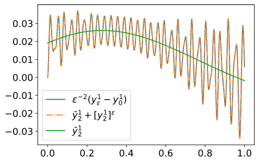
Refer to caption
(a) ε−2​(yε1​(t)−y01​(t))\varepsilon^{-2}(y_{\varepsilon}^{1}(t)-y_{0}^{1}(t)), y¯21​(t)+[y21]ε​(t)\bar{y}_{2}^{1}(t)+[y_{2}^{1}]^{\varepsilon}(t) and y¯21​(t)\bar{y}_{2}^{1}(t)
for t∈[0,1]t\in[0,1]
Refer to caption
(b) ε−2​(yε1​(t)−y01​(t))−(y¯21​(t)+[y21]ε​(t))\varepsilon^{-2}(y_{\varepsilon}^{1}(t)-y_{0}^{1}(t))-(\bar{y}_{2}^{1}(t)+[y_{2}^{1}]^{\varepsilon}(t))
for t∈[0,1]t\in[0,1]
Figure 2: Comparison of ε−2​(yε1​(t)−y01​(t))\varepsilon^{-2}(y_{\varepsilon}^{1}(t)-y_{0}^{1}(t)) and y¯21​(t)+[y21]ε​(t)\bar{y}_{2}^{1}(t)+[y_{2}^{1}]^{\varepsilon}(t) on a short time interval t∈[0,1]t\in[0,1], with yε1y_{\varepsilon}^{1}, y01y_{0}^{1} and y¯21\bar{y}_{2}^{1} as the solutions of (6a), (9) and (50), with ε=0.55\varepsilon=0.5^{5}. The function [y21]ε[y_{2}^{1}]^{\varepsilon} is given explicitly in Definition 5.1.

Although the error yε1−y01−ε2​[y¯21]εy_{\varepsilon}^{1}-y_{0}^{1}-\varepsilon^{2}[\bar{y}_{2}^{1}]^{\varepsilon} looks very accurate on short time intervals, the accuracy decreases, as Figure 2(b) suggest, for long time intervals. Figure 3 reveals how this error increases for long time intervals. Here, we integrated (6a), (9) and (50) for ε=0.53\varepsilon=0.5^{3}, where T=ε−2T=\varepsilon^{-2}.

Refer to caption
Figure 3: The second-order correction [y¯21]ε​(t)=y¯21​(t)+[y21]ε​(t)[\bar{y}_{2}^{1}]^{\varepsilon}(t)=\bar{y}_{2}^{1}(t)+[y_{2}^{1}]^{\varepsilon}(t) and its average motion y¯21​(t)\bar{y}_{2}^{1}(t) superimposed on y21​ε​(t)=ε−2​(yε1​(t)−y01​(t))y_{2}^{1\varepsilon}(t)=\varepsilon^{-2}(y_{\varepsilon}^{1}(t)-y_{0}^{1}(t)) for t∈[0,ε−2]t\in[0,\varepsilon^{-2}] where ε=0.53\varepsilon=0.5^{3}.

7.1 Comparison of the execution time

As mentioned earlier, the approximation of yε1y_{\varepsilon}^{1} by the homogenisation limit y01y_{0}^{1} comes with a trade-off. The simulation of y01y_{0}^{1} is faster than that of yε1y_{\varepsilon}^{1} but introduces an approximation error of order 𝒪⁡(ε2)\mathcal{O}(\varepsilon^{2}). This error can be reduced by approximating yε1y_{\varepsilon}^{1} by y01+ε2​[y¯21]εy_{0}^{1}+\varepsilon^{2}[\bar{y}_{2}^{1}]^{\varepsilon}, i.e., the second-order asymptotic expansion derived in Theorem 5.2. The leading-order and second-order errors are discussed in the previous section. We now discuss the computational costs of the simulations in this section.

Before comparing the total runtime for deriving yε1y_{\varepsilon}^{1}, y01y_{0}^{1} and y01+ε2​[y¯21]εy_{0}^{1}+\varepsilon^{2}[\bar{y}_{2}^{1}]^{\varepsilon}, we note that in [y¯21]ε=y¯21+[y21]ε[\bar{y}_{2}^{1}]^{\varepsilon}=\bar{y}_{2}^{1}+[y_{2}^{1}]^{\varepsilon}, the function y¯21\bar{y}_{2}^{1} traces the slow, average motion of the second-order correction term and is given as the solution to (50), while [y21]ε[y_{2}^{1}]^{\varepsilon} is the explicitly given rapidly oscillating term of the second-order correction. Moreover, we point out that the derivation of y01y_{0}^{1} and y¯21\bar{y}_{2}^{1} can be carried out in parallel. As such, there is little additional simulational overhead in computing the second-order asymptotic expansion [y¯21]ε[\bar{y}_{2}^{1}]^{\varepsilon}.

To analyse the execution time for simulating yε1y_{\varepsilon}^{1}, y01y_{0}^{1} and y01+ε2​[y¯21]εy_{0}^{1}+\varepsilon^{2}[\bar{y}_{2}^{1}]^{\varepsilon}, we determine the maximal step sizes such that certain convergence properties are still satisfied. More precisely, we determine the maximal step size d​t0,yε1maxdt_{0,y_{\varepsilon}^{1}}^{\max} to compute yε1y_{\varepsilon}^{1} and d​t0,y01maxdt_{0,y_{0}^{1}}^{\max} to compute y01y_{0}^{1} such that

(52) ‖yε1−y01‖L∞​([0,T])=𝒪⁡(ε2)\left\|y_{\varepsilon}^{1}-y_{0}^{1}\right\|_{L^{\infty}([0,T])}=\mathcal{O}(\varepsilon^{2})

and the maximal step size d​t2,yε1maxdt_{2,y_{\varepsilon}^{1}}^{\max} to compute yε1y_{\varepsilon}^{1} and d​t2,y01,y¯21maxdt_{2,y_{0}^{1},\bar{y}_{2}^{1}}^{\max} to compute y01y_{0}^{1} and y¯21\bar{y}_{2}^{1} such that

(53) ‖yε1−y01−ε2​[y¯21]ε‖L∞​([0,T])=𝒪⁡(ε3).\left\|y_{\varepsilon}^{1}-y_{0}^{1}-\varepsilon^{2}[\bar{y}^{1}_{2}]^{\varepsilon}\right\|_{L^{\infty}([0,T])}=\mathcal{O}(\varepsilon^{3}).

To determine, for instance, d​t2,yε1maxdt_{2,y_{\varepsilon}^{1}}^{\max}, we fix ε\varepsilon and derive y01y_{0}^{1} and y¯21\bar{y}_{2}^{1} with a small but fixed step size d​t2,y01,y¯21dt_{2,y_{0}^{1},\bar{y}_{2}^{1}}, and solve system (6a) for increasingly larger d​t2,yε1dt_{2,y_{\varepsilon}^{1}}. This process results in an error plot as shown in Figure 4. The error is constant for small step sizes d​t2,yε1dt_{2,y_{\varepsilon}^{1}} and increases after crossing an ε\varepsilon-dependent threshold value. This value expresses the maximal step size d​t2,yε1maxdt_{2,y_{\varepsilon}^{1}}^{\max} which still ensures that property (53) holds. A similar procedure was applied to determine the step size d​t0,yε1maxdt_{0,y_{\varepsilon}^{1}}^{\max} such that property (52) holds, and conversely to determine d​t0,y01maxdt_{0,y_{0}^{1}}^{\max} and d​t2,y01,y¯21maxdt_{2,y_{0}^{1},\bar{y}_{2}^{1}}^{\max}.

Refer to caption
Figure 4: Graphs of ‖y21​ε−[y¯21]ε‖L∞​([0,T])\left\|y_{2}^{1\varepsilon}-[\bar{y}_{2}^{1}]^{\varepsilon}\right\|_{L^{\infty}([0,T])} versus step-size d​t2,yε1dt_{2,y_{\varepsilon}^{1}} for different values of ε\varepsilon. The start of an upwards slope indicates the maximal step-size.

With this procedure, we find for ε=0.5k\varepsilon=0.5^{k} (k=2,…,7)(k=2,\ldots,7) the maximal step size such that the properties (52) and (53) are still satisfied. That is, for the leading-order error (52) we derive d0,yε1max=𝒪⁡(ε2)d_{0,y_{\varepsilon}^{1}}^{\max}=\mathcal{O}(\varepsilon^{2}) and d0,y01max=𝒪⁡(ε)d_{0,y_{0}^{1}}^{\max}=\mathcal{O}(\varepsilon), and for the second-order error (53) we obtain d​t2,yε1max=𝒪⁡(ε3)dt_{2,y_{\varepsilon}^{1}}^{\max}=\mathcal{O}(\varepsilon^{3}) and d​t2,y01,y¯21max=𝒪⁡(ε3/2)dt_{2,y_{0}^{1},\bar{y}_{2}^{1}}^{\max}=\mathcal{O}(\varepsilon^{3/2}). The exact maximal step sizes are listed in Tables 3 and 4 in Appendix B.

With these maximal step sizes, we can determine the average runtime for simulating yε1y_{\varepsilon}^{1}, y01y_{0}^{1} and y01+ε2​[y¯21]εy_{0}^{1}+\varepsilon^{2}[\bar{y}_{2}^{1}]^{\varepsilon} as depicted in Figures 5(a) and 5(b). Most significantly, we see that the derivation of the leading-order asymptotic expansion in Figure 5(a) and the second-order asymptotic expansion in Figure 5(b) are up to two orders of magnitude faster than the simulation of yε1y_{\varepsilon}^{1} via (6a). This directly reflects the differences in the maximal step sizes as explained above. Moreover, Figure 5(b) shows that the execution time for simulating y01y_{0}^{1} as the leading-order approximation and y¯21\bar{y}_{2}^{1} as the averaged second-order correction are comparable. The minimal difference can be explained by the evolution equation (50), which is more complicated than in (9), resulting in an increase of floating points operations per time-step.

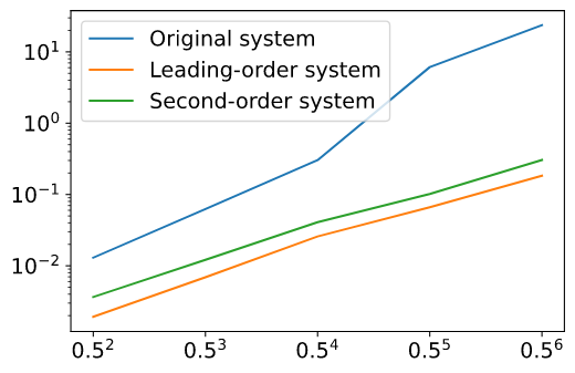
Refer to caption
(a) Average runtime in seconds to solve (6a) and (9) for different values of ε\varepsilon.
Refer to caption
(b) Average runtime in seconds to solve (6a), (9) and (50) for different values of ε\varepsilon.
Figure 5: Total runtime to simulate yε1y_{\varepsilon}^{1} from (6a), y01y_{0}^{1} from (9) and y¯21\bar{y}^{1}_{2} from (50). The exact computation times are given in Appendix B.

7.2 Details of the implementation

To compare the runtime of solving system (6a) for yεy_{\varepsilon} with an accuracy that describes its evolution up to second-order with both the leading-order approximation (Theorem 2.1) and second-order approximation (Theorem 5.2), one needs a numerical integration scheme that allows to solve each of the three systems of differential equations (6a), (9) and (50).

We note that system (6a) and (9) are given as two autonomous, second-order systems of differential equations. As such, a simple Velocity-Verlet algorithm, which is frequently used in the numerical integration of molecular dynamic systems, can be used to integrate these systems. However, system (50) is non-autonomous. Thus, a numerical integration scheme from the family of Runge–Kutta methods could be used to integrate each of the three systems of differential equations. We notice that system (50) resembles Hamilton’s canonical equations. In particular, the system is separable, which allows for the implementation of efficient partitioned Runge–Kutta methods. Furthermore, because of the Hamiltonian structure of systems (6a) and (9), it seems natural to apply a symplectic partitioned Runge–Kutta method as an integration scheme for solving the three systems. On that account, the simulations in this article were derived on the basis of a second-order symplectic partitioned Runge–Kutta method which combines the following Lobatto IIIA (Table 2) and Lobatto IIIB (Table 2) tableaux (taken from [10, Chapter IV.5]). Sun [28] proved (also see [12]), that this specific method is symplectic. A detailed description of the implementation can be found in [25, Chapter 8 and 14].

00 00 00
11 1/21/2 1/21/2
1/21/2 1/21/2
Table 1: Lobatto IIIA
00 1/21/2 00
11 1/21/2 00
1/21/2 1/21/2
Table 2: Lobatto IIIB

8 Conclusion

In this article, we studied a class of fast–slow Hamiltonian systems with energy functions given by

Eε=12​|y˙ε|2+12​|z˙ε|2+V⁡(yε)+12​ε−2​∑λ=1rωλ2​(yε)​(zελ)2,E_{\varepsilon}=\frac{1}{2}|\dot{y}_{\varepsilon}|^{2}+\frac{1}{2}|\dot{z}_{\varepsilon}|^{2}+V(y_{\varepsilon})+\frac{1}{2}\varepsilon^{-2}\sum_{\lambda=1}^{r}\omega_{\lambda}^{2}(y_{\varepsilon})(z_{\varepsilon}^{\lambda})^{2},

where yεjy_{\varepsilon}^{j} (j=1,…,n)(j=1,\ldots,n) are the slow and zελz_{\varepsilon}^{\lambda} (λ=1,…,r)(\lambda=1,\ldots,r) are the non-ergodic fast degrees of freedom and 0<ε<ε0<∞0<\varepsilon<\varepsilon_{0}<\infty is a parameter characterising their typical timescale ratio. A simplified version of one fast and one slow degree of freedom was already studied in [14].

In the first part of this article, we introduced a transformation of the fast degrees of freedom into action–angle variables (zε,z˙ε)↦(θε,ϕε)(z_{\varepsilon},\dot{z}_{\varepsilon})\mapsto(\theta_{\varepsilon},\phi_{\varepsilon}), which also required a transformation of the momenta y˙ε↦pε\dot{y}_{\varepsilon}\mapsto p_{\varepsilon}. We derived subsequently the second-order asymptotic expansion of the transformed degrees of freedom. Furthermore, we showed that these expansions can be decomposed into terms that oscillate rapidly around zero and slow terms that trace the average motion of the expansion. While the rapidly oscillating terms are given explicitly, the slow, average terms are given as solutions to an inhomogeneous linear system of differential equations.

In the second part of this article, we studied the fast subsystem characterised by the energy function

Eε⟂=12​|z˙ε|2+12​ε−2​∑λ=1rωλ2​(yε)​(zελ)2.E_{\varepsilon}^{\perp}=\frac{1}{2}|\dot{z}_{\varepsilon}|^{2}+\frac{1}{2}\varepsilon^{-2}\sum_{\lambda=1}^{r}\omega_{\lambda}^{2}(y_{\varepsilon})(z_{\varepsilon}^{\lambda})^{2}.

Guided by the thermodynamic theory for ergodic Hamiltonian systems described by Hertz, we regard the dynamics of the fast degrees of freedom zελz_{\varepsilon}^{\lambda} (λ=1,…,r)(\lambda=1,\ldots,r) as a system that is slowly perturbed by the interaction with the slow degrees of freedom yεjy_{\varepsilon}^{j} (j=1,…,n)(j=1,\ldots,n). Because the fast subsystem is not ergodic, we followed along the lines of [2] and replaced the time-average in classical statistical mechanics by an ensemble-average and defined otherwise, following Hertz, the temperature TεT_{\varepsilon}, the entropy SεS_{\varepsilon} and the external force FεF_{\varepsilon} of the fast subsystem.

Together with the second-order asymptotic expansion derived in the first part of this article, we expanded Eε⟂E_{\varepsilon}^{\perp}, TεT_{\varepsilon}, SεS_{\varepsilon} and FεF_{\varepsilon}. After analysing the leading-order asymptotic expansion of these terms, we found that they obey an energy relation akin to the first and second law of thermodynamics (in the sense of Carathéodory)

d​E0⟂=∑j=1nF0j​d​y0j+T0​d​S0.dE_{0}^{\perp}=\sum_{j=1}^{n}F_{0}^{j}dy_{0}^{j}+T_{0}dS_{0}.

In contrast to the case studied in [14], the entropy is not always constant. Indeed, the entropy is constant if and only if all weighted frequency ratios θ∗λ​ωλ​(y0)/ωμ​(y0)\theta_{\ast}^{\lambda}\omega_{\lambda}(y_{0})/\omega_{\mu}(y_{0}) (λ,μ=1,…,r)(\lambda,\mu=1,\ldots,r) are constant. In this case, the fast subsystem’s dynamics is a rigid (quasi-)periodic motion. We infer that, in the case of a constant entropy, the fast subsystem can be regarded as an adiabatic thermodynamic system, while in the case of a non-constant entropy, it can be interpreted as a non-adiabatic thermodynamic system.

Remarkably, for the second-order asymptotic expansion we find, for fixed (y0,p0)(y_{0},p_{0}), a thermodynamic energy relation of the form

d​E¯2⟂=∑j=1nF0j​d​y¯2j+T0​d​S¯2.d\bar{E}^{\perp}_{2}=\sum_{j=1}^{n}F_{0}^{j}d\bar{y}_{2}^{j}+T_{0}d\bar{S}_{2}.

With a second-order entropy expression S¯2\bar{S}_{2} that is not constant, we can interpret the averaged second-order asymptotic dynamics as a non-adiabatic thermodynamic process.

Finally, in the third part of this article, we analysed the model problem from a numerical point of view. In particular, we compared by means of a specific test model the quality of the short- and long-term approximation of yεy_{\varepsilon} by the leading-order asymptotic expansion y0y_{0} and by the second-order asymptotic expansion y0+ε2​[y¯2]εy_{0}+\varepsilon^{2}[\bar{y}_{2}]^{\varepsilon}. Most importantly we found that the time interval for which y0+ε2​[y¯2]εy_{0}+\varepsilon^{2}[\bar{y}_{2}]^{\varepsilon} ceases to be a viable approximation of yεy_{\varepsilon} is significantly longer than for an approximation by y0y_{0} alone. Moreover, we analysed in a series of tests how the total runtime of numerically computing yεy_{\varepsilon}, y0y_{0} and y¯2\bar{y}_{2} depends on the value of the scale parameter ε\varepsilon. We derived experimentally the largest step size so that certain convergence properties are still satisfied. In contrast to system (9) and (50), which only require the integration of slow degrees of freedom and thus allow for choosing a relatively large step size, the integration of system (6a) requires the choice of a relatively small step size to accurately replicate small-scale oscillations in the numerical solution. As a consequence, we found that the runtime for simulating y0y_{0} and y¯2\bar{y}_{2}, and thus for simulating the second-order asymptotic expansion y0+ε2​[y¯2]εy_{0}+\varepsilon^{2}[\bar{y}_{2}]^{\varepsilon}, is up to two orders of magnitude faster than the simulation of yεy_{\varepsilon} from the original system, for a similar accuracy.

The analysis of this article is restricted to a simple Hamiltonian. A significant limitation of the current analysis is the choice of the interaction potential UU in (4). The diagonal structure implies that fast modes interact only indirectly, through slow modes as intermediaries, via multiplicative coupling. Such a coupling appears in the Caldeira–Leggett Hamiltonian [5], with Lagrangian

ℒ⁡(y,z,y˙,z˙)=12​M​y˙2−V⁡(y)+12​∑λ=1rmλ​z˙λ2−12​∑λ=1rmλ​cλ​zλ2−y​∑λ=1rωλ​zλ\mathscr{L}(y,z,\dot{y},\dot{z})=\frac{1}{2}M\dot{y}^{2}-V(y)+\frac{1}{2}\sum_{\lambda=1}^{r}m_{\lambda}\dot{z}_{\lambda}^{2}-\frac{1}{2}\sum_{\lambda=1}^{r}m_{\lambda}c_{\lambda}z_{\lambda}^{2}-y\sum_{\lambda=1}^{r}\omega_{\lambda}z_{\lambda}

with cλ>0c_{\lambda}>0. (Note in the framework of this article, the small parameter would here not be the mass ratio mλ/Mm_{\lambda}/M, but the limit of increasing coupling ωλ\omega_{\lambda}.) For direct practical applications such as chemical reactions, for example, the evolution of the butane molecule, an extension of the results presented here to more complex potentials is required. One of the key insights of this paper is the existence of thermodynamic potentials far from equilibrium, albeit in the special situation of diagonal, or diagonalisable, interaction potentials UU. If this observation holds in greater generality, then this can lead to a better understanding and better computational approaches away from equilibrium, such as a chain of atoms linked to two reservoirs assigning the outer atoms different temperatures. This is a matter of future investigation.

Acknowledgements

We thank Ben Leimkuhler for stimulating discussions. MK is supported by a scholarship from the EPSRC Centre for Doctoral Training in Statistical Applied Mathematics at Bath (SAMBa), under the project EP/L015684/1. JZ gratefully acknowledges funding by a Royal Society Wolfson Research Merit Award. CR acknowledges support from NSF CAREER Award, United States, CMMI-2047506.

Appendix A Hertz’ approach to thermodynamics

As mentioned earlier, the authors in [14] analyse a simplified version of the model problem as presented in Section (2) from a thermodynamic point of view. More precisely, they focus on a system of one fast and one slow degree of freedom, i.e., n=r=1n=r=1, whose fast subsystem is by construction ergodic. That analysis builds on the thermodynamic theory described by Hertz as presented in [2]. Because of the similarity of the two models, we will focus on the differences in the derivation of the temperature, entropy and external force as given in (46) and refer the interested reader for a detailed discussion to [14].

A.1 Introduction to thermodynamics for non-ergodic systems

To illustrate the difference in the derivation of the thermodynamic quantities in [14] and here, we recall how the temperature is derived for the ergodic system studied in [14] and explain why the same approach fails for non-ergodic systems as studied in this article.

Let us start by analysing the dynamics of a generalised position zε∈ℝrz_{\varepsilon}\in\mathbb{R}^{r} and momentum ζε∈ℝr\zeta_{\varepsilon}\in\mathbb{R}^{r} governed by a Hamiltonian of the form

Hε⟂​(zε,ζε,yε)≔∑λ=1rHελ​(zε,ζε,yε),whereHελ​(zε,ζε,yε)≔12​(ζελ)2+12​ωλ2​(yε)​(zελ)2,λ=1,…,r,H_{\varepsilon}^{\perp}(z_{\varepsilon},\zeta_{\varepsilon};y_{\varepsilon})\coloneqq\sum_{\lambda=1}^{r}H_{\varepsilon}^{\lambda}(z_{\varepsilon},\zeta_{\varepsilon};y_{\varepsilon}),\qquad\text{where}\qquad H_{\varepsilon}^{\lambda}(z_{\varepsilon},\zeta_{\varepsilon};y_{\varepsilon})\coloneqq\frac{1}{2}(\zeta_{\varepsilon}^{\lambda})^{2}+\frac{1}{2}\omega_{\lambda}^{2}(y_{\varepsilon})(z_{\varepsilon}^{\lambda})^{2},\qquad\lambda=1,\ldots,r,

and yε​(t)=y⁡(ε​t)∈ℝny_{\varepsilon}(t)=y(\varepsilon t)\in\mathbb{R}^{n} are slow external parameters with y˙ε=𝒪⁡(ε)\dot{y}_{\varepsilon}=\mathcal{O}(\varepsilon). This setting of a Hamiltonian system which is slowly perturbed by an external parameter is fundamental in the thermodynamic formulation derived by Hertz. For ε=0\varepsilon=0, the unperturbed Hamiltonian is given by

H0⟂​(z0,ζ0,y0)=∑λ=1rH0λ​(z0,ζ0,y0),whereH0λ​(z0,ζ0,y0)=12​(ζ0λ)2+12​ωλ2​(y0)​(z0λ)2,λ=1,…,r,H_{0}^{\perp}(z_{0},\zeta_{0};y_{0})=\sum_{\lambda=1}^{r}H_{0}^{\lambda}(z_{0},\zeta_{0};y_{0}),\qquad\text{where}\qquad H_{0}^{\lambda}(z_{0},\zeta_{0};y_{0})=\frac{1}{2}(\zeta_{0}^{\lambda})^{2}+\frac{1}{2}\omega_{\lambda}^{2}(y_{0})(z_{0}^{\lambda})^{2},\qquad\lambda=1,\ldots,r,

and y0​(t)=y⁡(0)≡y∗y_{0}(t)=y(0)\equiv y_{\ast}. With initial values of the form z0λ​(0)=0z_{0}^{\lambda}(0)=0 and ζ0λ​(0)=2​E∗λ\zeta_{0}^{\lambda}(0)=\sqrt{2E_{\ast}^{\lambda}} the solutions to the corresponding Hamilton’s equations are then given for λ=1,…,r\lambda=1,\ldots,r by

(54) z0λ​(t)=2​E∗λωλ2​(y∗)​sin⁡(ωλ​(y∗)​t),ζ0λ​(t)=2​E∗λ​cos⁡(ωλ​(y∗)​t).z_{0}^{\lambda}(t)=\sqrt{\frac{2E^{\lambda}_{\ast}}{\omega^{2}_{\lambda}(y_{\ast})}}\sin\left(\omega_{\lambda}(y_{\ast})t\right),\qquad\zeta^{\lambda}_{0}(t)=\sqrt{2E^{\lambda}_{\ast}}\cos\left(\omega_{\lambda}(y_{\ast})t\right).

Moreover, we define the constant total energy

E∗⟂≔∑λ=1rE∗λ,whereE∗λ≔12​(ζ0λ)2+12​ωλ2​(y∗)​(z0λ)2,λ=1,…,r.E_{\ast}^{\perp}\coloneqq\sum_{\lambda=1}^{r}E_{\ast}^{\lambda},\qquad\text{where}\qquad E_{\ast}^{\lambda}\coloneqq\frac{1}{2}(\zeta_{0}^{\lambda})^{2}+\frac{1}{2}\omega_{\lambda}^{2}(y_{\ast})(z_{0}^{\lambda})^{2},\qquad\lambda=1,\ldots,r.

If r=1r=1, the trajectory of (z0,ζ0)(z_{0},\zeta_{0}) covers the entire energy surface {(z0,ζ0)∈ℝ2:H0⟂​(z0,ζ0,y0)=E∗⟂}\{(z_{0},\zeta_{0})\in\mathbb{R}^{2}\colon H_{0}^{\perp}(z_{0},\zeta_{0};y_{0})=E_{\ast}^{\perp}\}. Hence, the system is ergodic. In this case, which corresponds to the model studied in [14], the temperature in thermal equilibrium is defined via the time average, indicated by angle brackets ⟨⋅⟩\left\langle\cdot\right\rangle, of twice the kinetic energy. More precisely, we obtain

Tλ​(E∗λ,y∗)≔⟨ζ0λ​∂H0λ∂ζ0λ⟩=limθ→∞1θ​∫0θ2​E∗λ​cos2⁡(ωλ​(y∗)​t)​𝑑t=E∗λ,T_{\lambda}(E_{\ast}^{\lambda},y_{\ast})\coloneqq\left\langle\zeta_{0}^{\lambda}\frac{\partial H_{0}^{\lambda}}{\partial\zeta_{0}^{\lambda}}\right\rangle=\lim_{\theta\to\infty}\frac{1}{\theta}\int_{0}^{\theta}2E_{\ast}^{\lambda}\cos^{2}(\omega_{\lambda}(y_{\ast})t)\,\mathrm{d}t=E_{\ast}^{\lambda},

which is unique in the case r=1r=1.

However, if r>1r>1, the energies E∗λE_{\ast}^{\lambda} (λ=1,…,r)(\lambda=1,\ldots,r) form distinct integrals of motion. This implies that the system is non-ergodic. A naïve application of the definition of temperature above results in distinct temperature expressions that are unsuitable to describe the thermodynamic state of the whole system, because their values are in general path-dependent, i.e., Tλ=E∗λ≠E∗μ=TμT_{\lambda}=E_{\ast}^{\lambda}\neq E_{\ast}^{\mu}=T_{\mu} for λ≠μ\lambda\neq\mu (λ,μ=1,…,r)(\lambda,\mu=1,\ldots,r). Therefore, we define as in [2] the temperature for non-ergodic systems via the ensemble-average. This gives a unique measure for the thermodynamic state of the whole system.

A.1.1 The Birkhoff–Khinchin theorem for non-ergodic systems

A suitable expression for the temperature, which provides a unique measure for the whole system, can be derived if, in addition to averaging with respect to time, one averages with respect to all uniformly distributed initial values on the energy surface, making the temperature path-independent. This ensemble average allows us to define a temperature expression as a measure of the average kinetic motion of the whole system. We follow [2] for the definition of the ensemble average and its application to Hamiltonian systems. Let x=x⁡(t,x0)x=x(t,x_{0}) be the parametric form of the trajectory in phase-space starting at the point x0x_{0}. Then, the average value of some function ϕ\phi with respect to any phase trajectory x⁡(t)x(t), i.e.,

⟨ϕ⁡(x)⟩=limθ→∞1θ​∫0θϕ⁡(x⁡(t,x0))​𝑑t,\left\langle\phi(x)\right\rangle=\lim_{\theta\to\infty}\frac{1}{\theta}\int_{0}^{\theta}\phi(x(t,x_{0}))\,\mathrm{d}t,

depends, in general, on x0x_{0}. An ensemble of systems is given by varying initial data x0x_{0}, independent and identically distributed over the phase region E≤H⁡(x)≤E+Δ​EE\leq H(x)\leq E+\Delta E. The probability density of x0x_{0} in this region is constant and is equal to (Γ⁡(E+Δ​E)−Γ⁡(E))−1\left(\Gamma(E+\Delta E)-\Gamma(E)\right)^{-1}.

The ensemble average, E.A.⟨ϕ⟩E.A.\left\langle\phi\right\rangle, of the function ϕ\phi is defined by

E.A.⟨ϕ⟩≔limΔ​E→01Γ⁡(E+Δ​E)−Γ⁡(E)​∫E≤H⁡(x0)≤E+Δ​Elimθ→∞1θ​∫0θϕ⁡(x⁡(t,x0))​𝑑t​d​x0.E.A.\left\langle\phi\right\rangle\coloneqq\lim_{\Delta E\to 0}\frac{1}{\Gamma(E+\Delta E)-\Gamma(E)}\int_{E\leq H(x_{0})\leq E+\Delta E}\lim_{\theta\to\infty}\frac{1}{\theta}\int_{0}^{\theta}\phi(x(t,x_{0}))\,\mathrm{d}t\,\mathrm{d}x_{0}.

Suppose that the order of calculation of the integral over x0x_{0} and limθ→∞\lim_{\theta\to\infty} can be changed. Then

(55) E.A.⟨ϕ⟩=limΔ​E→01Γ⁡(E+Δ​E)−Γ⁡(E)​limθ→∞1θ​∫0θ∫E≤H⁡(x0)≤E+Δ​Eϕ⁡(x⁡(t,x0))​d​x0​𝑑t.E.A.\left\langle\phi\right\rangle=\lim_{\Delta E\to 0}\frac{1}{\Gamma(E+\Delta E)-\Gamma(E)}\lim_{\theta\to\infty}\frac{1}{\theta}\int_{0}^{\theta}\int_{E\leq H(x_{0})\leq E+\Delta E}\phi(x(t,x_{0}))\,\mathrm{d}x_{0}\,\mathrm{d}t.

The region E≤H⁡(x0)≤E+Δ​EE\leq H(x_{0})\leq E+\Delta E is invariant under the action of the phase flow x⁡(t,x0)x(t,x_{0}). Hence, in calculating the integral over x0x_{0} in (55), one can make a change of the variables x0↦xx_{0}\mapsto x. Since the determinant of this transformation is 11 by Liouville’s theorem, we can write

∫E≤H⁡(x0)≤E+Δ​Eϕ⁡(x⁡(t,x0))​d​x0=∫E≤H⁡(x)≤E+Δ​Eϕ⁡(x)​𝑑x.\int_{E\leq H(x_{0})\leq E+\Delta E}\phi(x(t,x_{0}))\,\mathrm{d}x_{0}=\int_{E\leq H(x)\leq E+\Delta E}\phi(x)\,\mathrm{d}x.

Thus, the integral does not depend on time. For small Δ​E\Delta E, this integral is given by

∫E≤H⁡(x)≤E+Δ​Eϕ⁡(x)​𝑑x≈Δ​E​∫ϕ⁡(x)​d​σ|∇H|.\int_{E\leq H(x)\leq E+\Delta E}\phi(x)\,\mathrm{d}x\approx\Delta E\int\phi(x)\frac{\,\mathrm{d}\sigma}{\left|\nabla H\right|}.

Therefore, we arrive at an “analogous” version of the Birkhoff–Khinchin theorem: for any Hamiltonian system

(56) E.A.⟨ϕ⟩=∫Σϕ⁡(x)​d​σ|∇H|∫Σd​σ|∇H|.E.A.\left\langle\phi\right\rangle=\frac{\int_{\Sigma}\phi(x)\frac{\,\mathrm{d}\sigma}{\left|\nabla H\right|}}{\int_{\Sigma}\frac{\,\mathrm{d}\sigma}{\left|\nabla H\right|}}.

This version of the Birkhoff–Khinchin theorem reflects the “average” (with respect to initial data) behaviour of non-ergodic Hamiltonian systems and is thus used to define the temperature in non-ergodic systems.

A.2 Derivation of thermodynamic relations in non-ergodic systems

As we saw in the previous section, the ensemble average of a function can be derived from the equality

E.A.⟨ϕ⟩=∫Σϕ⁡(x)​d​σ|∇H|∫Σd​σ|∇H|,E.A.\left\langle\phi\right\rangle=\frac{\int_{\Sigma}\phi(x)\frac{\,\mathrm{d}\sigma}{\left|\nabla H\right|}}{\int_{\Sigma}\frac{\,\mathrm{d}\sigma}{\left|\nabla H\right|}},

where Σ={(z0,ζ0)∈ℝ2​r:H0⟂​(z0,ζ0,y∗)=E∗⟂}\Sigma=\{(z_{0},\zeta_{0})\in\mathbb{R}^{2r}\colon H^{\perp}_{0}(z_{0},\zeta_{0};y_{\ast})=E^{\perp}_{\ast}\}, d​σ\,\mathrm{d}\sigma is a surface element on the energy surface and

|∇H0⟂|=[∑λ=1r(∂H0⟂∂ζ0λ)2+(∂H0⟂∂z0λ)2]1/2.|\nabla H^{\perp}_{0}|=\left[\sum_{\lambda=1}^{r}\left(\frac{\partial H^{\perp}_{0}}{\partial\zeta^{\lambda}_{0}}\right)^{2}+\left(\frac{\partial H^{\perp}_{0}}{\partial z^{\lambda}_{0}}\right)^{2}\right]^{1/2}.

The temperature for non-ergodic Hamiltonian systems is defined via the ensemble average by

(57) T⁡(E∗⟂,y∗)≔E.A.⟨ζ0λ​∂H0⟂​(z0,ζ0,y∗)∂ζ0λ⟩=∫Σζ0λ​∂H0⟂∂ζ0λ​d​σ|∇H0⟂|∫Σd​σ|∇H0⟂|.T(E^{\perp}_{\ast},y_{\ast})\coloneqq E.A.\left\langle\zeta^{\lambda}_{0}\frac{\partial H^{\perp}_{0}(z_{0},\zeta_{0};y_{\ast})}{\partial\zeta^{\lambda}_{0}}\right\rangle=\frac{\displaystyle\int_{\Sigma}\zeta^{\lambda}_{0}\frac{\partial H^{\perp}_{0}}{\partial\zeta^{\lambda}_{0}}\dfrac{\,\mathrm{d}\sigma}{|\nabla H^{\perp}_{0}|}}{\displaystyle\int_{\Sigma}\frac{\,\mathrm{d}\sigma}{|\nabla H^{\perp}_{0}|}}.

The numerator can be evaluated by noting that ∂H0⟂/∂ζ0λ\partial H^{\perp}_{0}/\partial\zeta^{\lambda}_{0} is the λ\lambdath component of the vector ∇H0⟂\nabla H^{\perp}_{0} and hence

nζλ≔∂H0⟂/∂ζ0λ|∇H0⟂|n^{\lambda}_{\zeta}\coloneqq\frac{\partial H^{\perp}_{0}/\partial\zeta^{\lambda}_{0}}{|\nabla H^{\perp}_{0}|}

is the λ\lambdath component of the outer unit vector n=∇H0⟂/|∇H0⟂|n=\nabla H^{\perp}_{0}/|\nabla H^{\perp}_{0}| on the energy surface. Therefore, we can write the numerator in the form

(58) ∫Σζ0λ​∂H0⟂∂ζ0λ​d​σ|∇H0⟂|=∫Σζ0λ​nζλ​𝑑σ=∫H0⟂​(z0,ζ0,y∗)≤E∗⟂dn​(z0,ζ0)≕Γ⁡(E∗⟂,y∗),\int_{\Sigma}\zeta^{\lambda}_{0}\frac{\partial H^{\perp}_{0}}{\partial\zeta^{\lambda}_{0}}\dfrac{\,\mathrm{d}\sigma}{|\nabla H^{\perp}_{0}|}=\int_{\Sigma}\zeta^{\lambda}_{0}n^{\lambda}_{\zeta}\,\mathrm{d}\sigma=\int_{H^{\perp}_{0}(z_{0},\zeta_{0};y_{\ast})\leq E^{\perp}_{\ast}}\,\mathrm{d}^{n}(z_{0},\zeta_{0})\eqqcolon\Gamma(E^{\perp}_{\ast},y_{\ast}),

which follows from Gauss’ theorem, where Γ⁡(E∗⟂,y∗)\Gamma(E^{\perp}_{\ast},y_{\ast}) is the phase-space volume enclosed by the trajectories of (54). To derive the denominator in (57), we calculate the derivative of Γ⁡(E∗⟂,y∗)\Gamma(E^{\perp}_{\ast},y_{\ast}) with respect to E∗⟂E^{\perp}_{\ast} and find

Γ⁡(E∗⟂+Δ​E∗⟂,y∗)−Γ⁡(E∗⟂,y∗)=∫E∗⟂≤H0⟂​(z0,ζ0,y∗)≤E∗⟂+Δ​E∗⟂dn​(z0,ζ0)≈∫H0⟂​(z0,ζ0,y∗)=E∗⟂Δ​n​𝑑σ,\Gamma(E^{\perp}_{\ast}+\Delta E^{\perp}_{\ast},y_{\ast})-\Gamma(E^{\perp}_{\ast},y_{\ast})=\int_{E^{\perp}_{\ast}\leq H^{\perp}_{0}(z_{0},\zeta_{0};y_{\ast})\leq E^{\perp}_{\ast}+\Delta E^{\perp}_{\ast}}\,\mathrm{d}^{n}(z_{0},\zeta_{0})\approx\int_{H^{\perp}_{0}(z_{0},\zeta_{0};y_{\ast})=E^{\perp}_{\ast}}\Delta n\,\mathrm{d}\sigma,

where Δ​n\Delta n is the distance between the energy surface H0⟂​(z0+nz​Δ​n,ζ0+nζ​Δ​n,y∗)=E∗⟂+Δ​E∗⟂H^{\perp}_{0}(z_{0}+n_{z}\Delta n,\zeta_{0}+n_{\zeta}\Delta n;y_{\ast})=E^{\perp}_{\ast}+\Delta E^{\perp}_{\ast} and H0⟂​(z0,ζ0,y∗)=E∗⟂H^{\perp}_{0}(z_{0},\zeta_{0};y_{\ast})=E^{\perp}_{\ast}. A Taylor expansion gives Δ​n=Δ​E∗⟂/|∇H0⟂|\Delta n=\Delta E^{\perp}_{\ast}/|\nabla H^{\perp}_{0}| and hence

(59) ∂Γ⁡(E∗⟂,y∗)∂E∗⟂=∫H0⟂​(z0,ζ0,y∗)=E∗⟂d​σ|∇H0⟂|.\frac{\partial\Gamma(E^{\perp}_{\ast},y_{\ast})}{\partial E^{\perp}_{\ast}}=\int_{H^{\perp}_{0}(z_{0},\zeta_{0};y_{\ast})=E^{\perp}_{\ast}}\frac{\,\mathrm{d}\sigma}{|\nabla H^{\perp}_{0}|}.

Combining Equations (57)–(59), the temperature TT can thus be expressed in terms of the phase-space volume Γ⁡(E∗⟂,y∗)\Gamma(E^{\perp}_{\ast},y_{\ast}):

(60) T⁡(E∗⟂,y∗)=Γ⁡(E∗⟂,y∗)∂Γ⁡(E∗⟂,y∗)/∂E∗⟂.T(E^{\perp}_{\ast},y_{\ast})=\frac{\Gamma(E^{\perp}_{\ast},y_{\ast})}{\partial\Gamma(E^{\perp}_{\ast},y_{\ast})/\partial E^{\perp}_{\ast}}.

Similar to [14] we integrate (60) with respect to E∗⟂E^{\perp}_{\ast} and obtain for the entropy

S⁡(E∗⟂,y∗)=log⁡(Γ⁡(E∗⟂,y∗))+f⁡(y∗),S(E^{\perp}_{\ast},y_{\ast})=\log\left(\Gamma(E^{\perp}_{\ast},y_{\ast})\right)+f(y_{\ast}),

where f⁡(y∗)f(y_{\ast}) is a constant of integration with respect to E∗⟂E_{\ast}^{\perp}. To find the dependence of SS on y∗y_{\ast} we follow again the derivation presented in [14]. Using (56), we calculate for j=1,…,nj=1,\ldots,n the external force

(61) Fj​(E∗⟂,y∗)=E.A.⟨∂H0⟂​(z0,ζ0,y∗)∂y∗j⟩=∫Σ∂H0⟂∂y∗j​d​σ|∇H0⟂|∫Σd​σ|∇H0⟂|.F_{j}(E^{\perp}_{\ast},y_{\ast})=E.A.\left\langle\frac{\partial H^{\perp}_{0}(z_{0},\zeta_{0};y_{\ast})}{\partial y^{j}_{\ast}}\right\rangle=\frac{\displaystyle\int_{\Sigma}\frac{\partial H^{\perp}_{0}}{\partial y^{j}_{\ast}}\dfrac{\,\mathrm{d}\sigma}{|\nabla H^{\perp}_{0}|}}{\displaystyle\int_{\Sigma}\frac{\,\mathrm{d}\sigma}{|\nabla H^{\perp}_{0}|}}.

For the numerator, we calculate the derivative of Γ⁡(E∗⟂,y∗)\Gamma(E^{\perp}_{\ast},y_{\ast}) with respect to y∗jy^{j}_{\ast}. Similarly to before, we have

Γ⁡(E∗⟂,y∗+Δ​y∗)−Γ⁡(E∗⟂,y∗)\displaystyle\Gamma(E^{\perp}_{\ast},y_{\ast}+\Delta y_{\ast})-\Gamma(E^{\perp}_{\ast},y_{\ast}) =\displaystyle= ∫H0⟂​(z0,ζ0,y∗+Δ​y∗)≤E∗⟂dn​(z0,ζ0)−∫H0⟂​(z0,ζ0,y∗)≤E∗⟂dn​(z0,ζ0)\displaystyle\int_{H^{\perp}_{0}(z_{0},\zeta_{0};y_{\ast}+\Delta y_{\ast})\leq E^{\perp}_{\ast}}\,\mathrm{d}^{n}(z_{0},\zeta_{0})-\int_{H^{\perp}_{0}(z_{0},\zeta_{0};y_{\ast})\leq E^{\perp}_{\ast}}\,\mathrm{d}^{n}(z_{0},\zeta_{0})
≈\displaystyle\approx ∫H0⟂​(z0,ζ0,y∗)=E∗⟂Δ​n​𝑑σ,\displaystyle\int_{H^{\perp}_{0}(z_{0},\zeta_{0};y_{\ast})=E^{\perp}_{\ast}}\Delta n\,\mathrm{d}\sigma,

where Δ​n\Delta n indicates the distance between the energy surface H0⟂​(z0+nz​Δ​n,ζ0+nζ​Δ​n,y∗j+Δ​y∗j)=E∗⟂H^{\perp}_{0}(z_{0}+n_{z}\Delta n,\zeta_{0}+n_{\zeta}\Delta n;y^{j}_{\ast}+\Delta y^{j}_{\ast})=E^{\perp}_{\ast} and H0⟂​(z0,ζ0,y∗)=E∗⟂H^{\perp}_{0}(z_{0},\zeta_{0};y_{\ast})=E^{\perp}_{\ast}. A Taylor expansion gives

Δ​n=−1|∇H0⟂|​∂H0⟂∂y∗j​Δ​y∗j\Delta n=-\frac{1}{|\nabla H^{\perp}_{0}|}\frac{\partial H^{\perp}_{0}}{\partial y^{j}_{\ast}}\Delta y^{j}_{\ast}

and we obtain

(62) ∂Γ⁡(E∗⟂,y∗)∂y∗j=−∫H0⟂​(z0,ζ0,y∗)=E∗⟂∂H0⟂∂y∗jd​σ|∇H0⟂|.\frac{\partial\Gamma(E^{\perp}_{\ast},y_{\ast})}{\partial y^{j}_{\ast}}=-\int_{H^{\perp}_{0}(z_{0},\zeta_{0};y_{\ast})=E^{\perp}_{\ast}}\frac{\partial H^{\perp}_{0}}{\partial y^{j}_{\ast}}\frac{\,\mathrm{d}\sigma}{|\nabla H^{\perp}_{0}|}.

Combining Equations (59), (61) and (62) we obtain

(63) Fj​(E∗⟂,y∗)=E.A.⟨∂H0⟂∂y∗j⟩=−∂Γ⁡(E∗⟂,y∗)/∂y∗j∂Γ⁡(E∗⟂,y∗)/∂E∗⟂.F_{j}(E^{\perp}_{\ast},y_{\ast})=E.A.\left\langle\frac{\partial H^{\perp}_{0}}{\partial y^{j}_{\ast}}\right\rangle=-\frac{\partial\Gamma(E^{\perp}_{\ast},y_{\ast})/\partial y^{j}_{\ast}}{\partial\Gamma(E^{\perp}_{\ast},y_{\ast})/\partial E^{\perp}_{\ast}}.

We thus find

(64) S⁡(E∗⟂,y∗)=log⁡(Γ⁡(E∗⟂,y∗))+C.S(E^{\perp}_{\ast},y_{\ast})=\log\left(\Gamma(E^{\perp}_{\ast},y_{\ast})\right)+C.

The constant CC is chosen such that the entropy is dimensionless. This is the key result of Hertz’ thermodynamic formulation: the explicit derivation of the entropy of a Hamiltonian system under the influence of a slowly varying parameter is (up to a constant) the logarithm of the phase-space volume.

A.3 Application to the model problem

The analysis of the previous section reveals that thermodynamic properties of Hamiltonian systems are intrinsically connected to the phase-space volume.

In general, the set {x∈ℝd:xT​Σ−1​x≤R2}\{x\in\mathbb{R}^{d}:x^{T}\Sigma^{-1}x\leq R^{2}\}, where Σ=diag⁡(a12,a22,…,ad2)\Sigma=\mathrm{diag}(a_{1}^{2},a_{2}^{2},\ldots,a_{d}^{2}) with a1,…,ad∈ℝa_{1},\ldots,a_{d}\in\mathbb{R}, describes a hyperellipsoid in ℝd\mathbb{R}^{d}. Its dd-dimensional volume is given by

(65) Γ=Γd​|Σ|1/2​Rd,\Gamma=\Gamma_{d}|\Sigma|^{1/2}R^{d},

where Γd\Gamma_{d} is the volume of the dd-dimensional hypersphere.

To calculate the phase-space volume for the model problem as presented in Section 2 note, that the set {(z0,ζ0)∈ℝ2​r:H0⟂​(z0,ζ0,y∗)=E∗⟂}\{(z_{0},\zeta_{0})\in\mathbb{R}^{2r}\colon H^{\perp}_{0}(z_{0},\zeta_{0};y_{\ast})=E^{\perp}_{\ast}\} with

(66) E∗⟂=∑λ=1rE∗λ=∑λ=1r12​(ζ0λ)2+12​ωλ2​(y∗)​(z0λ)2,E^{\perp}_{\ast}=\sum_{\lambda=1}^{r}E_{\ast}^{\lambda}=\sum_{\lambda=1}^{r}\frac{1}{2}(\zeta_{0}^{\lambda})^{2}+\frac{1}{2}\omega_{\lambda}^{2}(y_{\ast})(z_{0}^{\lambda})^{2},

describes a hyperellipsoid in ℝ2​r\mathbb{R}^{2r}. Equation (66) can be written in the form E∗⟂=xT​Σ−1​xE^{\perp}_{\ast}=x^{T}\Sigma^{-1}x with x=(z01,z02,…,z0r,ζ01,ζ02,…,ζ0r)x=(z_{0}^{1},z_{0}^{2},\ldots,z_{0}^{r},\zeta_{0}^{1},\zeta_{0}^{2},\ldots,\zeta_{0}^{r}) and

Σ=diag⁡(2,2,…,2,2ω12​(y∗),2ω22​(y∗),…,2ωr2​(y∗)).\Sigma=\mathrm{diag}\left(2,2,\ldots,2,\frac{2}{\omega^{2}_{1}(y_{\ast})},\frac{2}{\omega^{2}_{2}(y_{\ast})},\ldots,\frac{2}{\omega^{2}_{r}(y_{\ast})}\right).

Therefore, with d=2​rd=2r and R2=E∗⟂R^{2}=E_{\ast}^{\perp}, the volume of the hyperellipsoid (66) is according to (65) given by

Γ⁡(E∗⟂,y∗)=Γ2​r​(2​E∗⟂)r∏λ=1rωλ​(y∗).\Gamma(E_{\ast}^{\perp},y_{\ast})=\Gamma_{2r}\frac{\left(2E_{\ast}^{\perp}\right)^{r}}{\prod_{\lambda=1}^{r}\omega_{\lambda}(y_{\ast})}.

We reason by analogy that the ε\varepsilon-dependent phase-space volume, characterised by the energy of the fast subsystem

Eε⟂=∑λ=1rEελ=∑λ=1r12​(ζελ)2+12​ε−2​ωλ2​(yε)​(zελ)2,E_{\varepsilon}^{\perp}=\sum_{\lambda=1}^{r}E_{\varepsilon}^{\lambda}=\sum_{\lambda=1}^{r}\frac{1}{2}(\zeta_{\varepsilon}^{\lambda})^{2}+\frac{1}{2}{\varepsilon}^{-2}\omega_{\lambda}^{2}(y_{\varepsilon})(z_{\varepsilon}^{\lambda})^{2},

is given by

(67) Γε​(Eε⟂,yε)=εr​Γ2​r​(2​Eε⟂)r∏λ=1rωλ​(yε).\Gamma_{\varepsilon}(E_{\varepsilon}^{\perp},y_{\varepsilon})=\varepsilon^{r}\Gamma_{2r}\frac{\left(2E_{\varepsilon}^{\perp}\right)^{r}}{\prod_{\lambda=1}^{r}\omega_{\lambda}(y_{\varepsilon})}.

We therefore define, provided that Γε​(Eε⟂,yε)≠0\Gamma_{\varepsilon}(E^{\perp}_{\varepsilon},y_{\varepsilon})\neq 0, the temperature, normalised entropy and external force, in analogy to (60), (63) and (64), as

Tε​(Eε⟂,yε)≔Γε​(Eε⟂,yε)∂Γε​(Eε⟂,yε)/∂Eε⟂,Sε​(Eε⟂,yε)≔log⁡(Γε​(Eε⟂,yε))+Cε,Fεj​(Eε⟂,yε)≔−∂Γε​(Eε⟂,yε)/∂yεj∂Γε​(Eε⟂,yε)/∂Eε⟂,T_{\varepsilon}(E_{\varepsilon}^{\perp},y_{\varepsilon})\coloneqq\frac{\Gamma_{\varepsilon}(E^{\perp}_{\varepsilon},y_{\varepsilon})}{\partial\Gamma_{\varepsilon}(E^{\perp}_{\varepsilon},y_{\varepsilon})/\partial E^{\perp}_{\varepsilon}},\quad S_{\varepsilon}(E_{\varepsilon}^{\perp},y_{\varepsilon})\coloneqq\log\left(\Gamma_{\varepsilon}(E^{\perp}_{\varepsilon},y_{\varepsilon})\right)+C_{\varepsilon},\quad F_{\varepsilon}^{j}(E_{\varepsilon}^{\perp},y_{\varepsilon})\coloneqq-\frac{\partial\Gamma_{\varepsilon}(E^{\perp}_{\varepsilon},y_{\varepsilon})/\partial y^{j}_{\varepsilon}}{\partial\Gamma_{\varepsilon}(E^{\perp}_{\varepsilon},y_{\varepsilon})/\partial E^{\perp}_{\varepsilon}},

which become with (67) and Cε=−log⁡((2​ε)r​Γ2​r)C_{\varepsilon}=-\log((2\varepsilon)^{r}\Gamma_{2r}) for j=1,…,nj=1,\ldots,n

Tε=1r​∑λ=1rθελ​ωλ​(yε),Sε=∑λ=1rlog⁡(Eε⟂ωλ​(yε)),Fεj=Tε​∑λ=1rDj​Lελ.T_{\varepsilon}=\frac{1}{r}\sum_{\lambda=1}^{r}\theta_{\varepsilon}^{\lambda}\omega_{\lambda}(y_{\varepsilon}),\qquad S_{\varepsilon}=\sum_{\lambda=1}^{r}\log\left(\frac{E_{\varepsilon}^{\perp}}{\omega_{\lambda}(y_{\varepsilon})}\right),\qquad F_{\varepsilon}^{j}=T_{\varepsilon}\sum_{\lambda=1}^{r}D_{j}L_{\varepsilon}^{\lambda}.

Appendix B Computation times for numerical simulations

For completeness, we present in this section the total computation times corresponding to the maximal step sizes used in the simulations presented in this article. Tables 3 and 4 illustrate in column yε1y_{\varepsilon}^{1} the total runtime for simulations of system (6a) with respect to distinct values of ε\varepsilon and a corresponding maximal step size as discussed in Section 7.1. Similarly, the columns y01y_{0}^{1} and y¯21\bar{y}_{2}^{1} indicate the total runtime for simulating systems (9) and (50). We recall that the maximal step size as discussed in Section 7.1 is given for the leading-order approximation under the theoretical global error (52) by d​t0,yε1max=𝒪⁡(ε2)dt_{0,y_{\varepsilon}^{1}}^{\max}=\mathcal{O}(\varepsilon^{2}) and d​t0,y01max=𝒪⁡(ε)dt_{0,y_{0}^{1}}^{\max}=\mathcal{O}(\varepsilon), and for the second-order approximation under the theoretical global error (53) by d​t2,yε1max=𝒪⁡(ε3)dt_{2,y_{\varepsilon}^{1}}^{\max}=\mathcal{O}(\varepsilon^{3}) and d​t2,y01,y¯21max=𝒪⁡(ε3/2)dt_{2,y_{0}^{1},\bar{y}_{2}^{1}}^{\max}=\mathcal{O}(\varepsilon^{3/2}). Note that we always chose identical step sizes for the derivation of y01y_{0}^{1} and y¯21\bar{y}_{2}^{1}.

The source code for the numerical integration scheme was written in Python version 3.8.5. The simulations of the systems (6a), (9) and (50) as presented in Tables 3 and 4 were performed on a single core Intel® Core™ i5-8250U CPU.

Computation times (s) and maximal step-sizes
ε\varepsilon 00yε1y_{\varepsilon}^{1} 00d​t0,yε1maxdt_{0,y_{\varepsilon}^{1}}^{\max} 00y01y_{0}^{1} 00d​t0,y01maxdt_{0,y_{0}^{1}}^{\max}
0.520.5^{2} 000.0026 001×10−21\times 10^{-2} 000.00028 006×10−26\times 10^{-2}
0.530.5^{3} 000.0271 001×10−31\times 10^{-3} 000.00059 003×10−23\times 10^{-2}
0.540.5^{4} 000.0488 005×10−45\times 10^{-4} 000.00182 001×10−21\times 10^{-2}
0.550.5^{5} 000.2392 001×10−41\times 10^{-4} 000.00266 007×10−37\times 10^{-3}
0.560.5^{6} 000.7945 003×10−53\times 10^{-5} 000.00590 003×10−33\times 10^{-3}
Table 3: Computation times in seconds for yε1y_{\varepsilon}^{1} and its leading-order asymptotic expansion y01y_{0}^{1} for maximally viable step-sizes that satisfy the theoretical global error (52).
Computation times (s) and maximal step-sizes
ε\varepsilon yε1y_{\varepsilon}^{1} d​t2,yε1maxdt_{2,y_{\varepsilon}^{1}}^{\max} y01y_{0}^{1} y¯21\bar{y}_{2}^{1} d​t2,y01,y¯21maxdt_{2,y_{0}^{1},\bar{y}_{2}^{1}}^{\max}
0.520.5^{2} 00.013 2×10⁻³²\times 10^{-3} 0.0019 0.0037 1×10⁻²¹\times 10^{-2}
0.530.5^{3} 00.062 4×10−44\times 10^{-4} 0.0069 0.0121 3×10⁻³³\times 10^{-3}
0.540.5^{4} 00.303 8×10−58\times 10^{-5} 0.0258 0.0408 8×10−48\times 10^{-4}
0.550.5^{5} 06.122 4×10−64\times 10^{-6} 0.0663 0.1017 3×10−43\times 10^{-4}
0.560.5^{6} 23.670 1×10−61\times 10^{-6} 0.1838 0.3041 1×10−41\times 10^{-4}
Table 4: Computation times in seconds for yε1y_{\varepsilon}^{1}, its leading-order asymptotic expansion y01y_{0}^{1} and averaged second-order correction y¯21\bar{y}_{2}^{1} for maximally viable step-sizes that satisfy the theoretical global error (53). The step-sizes for deriving y01y_{0}^{1} and y¯21\bar{y}_{2}^{1} are chosen the same.

References

  • [1] V.. Arnol’d “Mathematical methods of classical mechanics” Translated from the 1974 Russian original by K. Vogtmann and A. Weinstein, Corrected reprint of the second (1989) edition 60, Graduate Texts in Mathematics Springer-Verlag, New York, 1989
  • [2] Victor. Berdichevsky “Thermodynamics of chaos and order” 90, Pitman Monographs and Surveys in Pure and Applied Mathematics Longman, Harlow, 1997
  • [3] Folkmar Bornemann “Homogenization in time of singularly perturbed mechanical systems” Revised version as of Aug 1998. http://www-m3.ma.tum.de/foswiki/pub/M3/Allgemeines/FolkmarBornemannPublications/Habil.pdf 1687, Lecture Notes in Mathematics Springer-Verlag, Berlin, 1998
  • [4] Folkmar. Bornemann and Christof Schütte “Homogenization of Hamiltonian systems with a strong constraining potential” In Physica D. Nonlinear Phenomena 102.1-2, 1997, pp. 57–77
  • [5] A.. Caldeira and A.. Leggett “Influence of Dissipation on Quantum Tunneling in Macroscopic Systems” In Physical Review Letters 46.4 American Physical Society (APS), 1981, pp. 211–214 DOI: 10.1103/physrevlett.46.211
  • [6] Sabyasachi Chatterjee, Amit Acharya and Zvi Artstein “Computing singularly perturbed differential equations” In Journal of Computational Physics 354, 2018, pp. 417–446 DOI: 10.1016/j.jcp.2017.10.025
  • [7] Sabyasachi Chatterjee et al. “Plasticity without phenomenology: A first step” In Journal of the Mechanics and Physics of Solids 143, 2020 DOI: 10.1016/j.jmps.2020.104059
  • [8] J.W. Gibbs “Elementary Principles in Statistical Mechanics: Developed with Especial Reference to the Rational Foundations of Thermodynamics” C. Scribner’s sons, 1902
  • [9] David Gilbarg and Neil. Trudinger “Elliptic partial differential equations of second order” Reprint of the 1998 edition, Classics in Mathematics Springer-Verlag, Berlin, 1983
  • [10] E. Hairer and G. Wanner “Solving ordinary differential equations. II” Stiff and differential-algebraic problems 14, Springer Series in Computational Mathematics Springer-Verlag, Berlin, 1991
  • [11] Paul Hertz “Über die mechanischen Grundlagen der Thermodynamik” In Annalen der Physik 338.12 Wiley, 1910, pp. 225–274537–552
  • [12] Laurent Jay “Symplectic partitioned Runge-Kutta methods for constrained Hamiltonian systems” In SIAM Journal on Numerical Analysis 33.1 Society for Industrial & Applied Mathematics (SIAM), 1996, pp. 368–387
  • [13] Zhidong Jia and Benedict. Leimkuhler “A projective thermostatting dynamics technique” In Multiscale Modeling & Simulation 4.2, 2005, pp. 563–583 DOI: 10.1137/040603863
  • [14] Matthias Klar, Karsten Matthies and Johannes Zimmer “Emergence of a nonconstant entropy for a fast-slow Hamiltonian system in its second-order asymptotic expansion”, 2020 arXiv:2010.10971 [math-ph]
  • [15] Christian Kuehn “Multiple time scale dynamics” 191, Applied Mathematical Sciences Springer, Cham, 2015 DOI: 10.1007/978-3-319-12316-5
  • [16] L.. Lerman and E.. Yakovlev “Geometry of slow-fast Hamiltonian systems and Painlevé equations” In Indagationes Mathematicae. New Series 27.5, 2016, pp. 1219–1244 DOI: 10.1016/j.indag.2016.09.003
  • [17] Xiaoguai Li and Celia Reina “Simultaneous spatial and temporal coarse-graining: from atomistic models to continuum elastodynamics” In Journal of the Mechanics and Physics of Solids 130 Elsevier BV, 2019, pp. 118–140
  • [18] D.. Mitrinović, J.. Pečarić and A.. Fink “Inequalities involving functions and their integrals and derivatives” 53, Mathematics and its Applications (East European Series) Kluwer Academic Publishers Group, Dordrecht, 1991
  • [19] Anatoly Neishtadt “Averaging method for systems with separatrix crossing” In Nonlinearity 30.7, 2017, pp. 2871–2917 DOI: 10.1088/1361-6544/aa712f
  • [20] Anatoly Neishtadt “On mechanisms of destruction of adiabatic invariance in slow-fast Hamiltonian systems” In Nonlinearity 32.11, 2019, pp. R53–R76 DOI: 10.1088/1361-6544/ab2a2c
  • [21] Grigorios. Pavliotis and Andrew. Stuart “Multiscale methods” Averaging and homogenization 53, Texts in Applied Mathematics Springer, New York, 2008, pp. xviii+307
  • [22] Sebastian Reich “Dynamical Systems, Numerical Integration, and Exponentially Small Estimates” Habilitationsschrift, Freie Universitat Berlin, ZIB-Report SC-98-19, 1998
  • [23] Sebastian Reich “Smoothed Langevin dynamics of highly oscillatory systems” In Physica D. Nonlinear Phenomena 138.3-4, 2000, pp. 210–224 DOI: 10.1016/S0167-2789(99)00200-6
  • [24] J.. Sanders, F. Verhulst and J. Murdock “Averaging methods in nonlinear dynamical systems” 59, Applied Mathematical Sciences Springer, New York, 2007
  • [25] J.. Sanz-Serna and M.. Calvo “Numerical Hamiltonian problems” 7, Applied Mathematics and Mathematical Computation Chapman & Hall, London, 1994
  • [26] Kushal Shah, Dmitry Turaev, Vassili Gelfreich and Vered Rom-Kedar “Equilibration of energy in slow–fast systems” Proceedings of the National Academy of Sciences, 2017 DOI: 10.1073/pnas.1706341114
  • [27] Elias. Stein “Harmonic analysis: real-variable methods, orthogonality, and oscillatory integrals” With the assistance of Timothy S. Murphy, Monographs in Harmonic Analysis, III 43, Princeton Mathematical Series Princeton University Press, Princeton, NJ, 1993
  • [28] Geng Sun “Symplectic partitioned Runge-Kutta methods” In Journal of Computational Mathematics 11.4, 1993, pp. 365–372
  • [29] Gerald Teschl “Ordinary differential equations and dynamical systems” 140, Graduate Studies in Mathematics American Mathematical Society, Providence, RI, 2012
  • [30] J.. Weiner “Statistical Mechanics of Elasticity” Dover Publications, 2002
  • [31] Stephen Wiggins “Introduction to applied nonlinear dynamical systems and chaos” 2, Texts in Applied Mathematics Springer-Verlag, New York, 2003