Collective excitations of superfluid Fermi gases near the transition temperature
Abstract
Studying the collective pairing phenomena in a two-component Fermi gas, we predict the appearance near the transition temperature of a well-resolved collective mode of quadratic dispersion. The mode is visible both above and below in the system’s response to a driving pairing field. When approaching from below, the phononic and pair-breaking branches, characteristic of the zero temperature behavior, reduce to a relatively low energy-momentum region, where they are replaced by the quadratically-dispersed pairing resonance, which thus acts as a precursor of the phase transition. In the strong-coupling and Bose-Einstein Condensate regime, this mode is a weakly-damped propagating mode associated to a Lorentzian resonance. Conversely, in the BCS limit it is a relaxation mode of pure imaginary eigenenergy. At large momenta, the resonance disappears when it is reabsorbed by the lower-edge of the pairing continuum. At intermediate temperatures between 0 and , we unify the newly found collective phenomena near with the phononic and pair-breaking branches predicted from previous studies, and we exhaustively classify the roots of the analytically continued dispersion equation, and show that they provided a very good summary of the pair spectral functions.
I Introduction
The present theoretical investigation is devoted to oscillation-like and relaxation-like collective excitations of atomic Fermi superfluids (see, for review, Ref. Strinati2018; Turlapov) in the crossover between the Bardeen-Cooper-Schrieffer (BCS) pairing regime and the opposite limit of the Bose-Einstein condensation (BEC) of molecules. An increasing interest to collective excitations in condensed Fermi gases has been recently inspired by experimental achievements Bartenstein; Kinast; Altmeyer; Tey; Sidorenkov; Hoinka; Kuhn2020. Particularly, in Refs. Hoinka; Kuhn2020, the spectral function of the density response of a Fermi gas has been experimentally investigated at finite momentum and temperature.
The state-of the art of the theory of collective excitations in atomic Fermi gases shows that there are still unexplored areas, in particular away from the low-temperature, low-momentum regime. Combescot et al. Combescot2006 and Diener et al. Diener2008 analyzed the dispersion of phononic (Anderson-Bogoliubov) collective excitations in a wide range of momentum at zero temperature. An analytic study of the dispersion of phonons has been performed in Ref. Kurkjian2016, still at . Ohashi and Griffin Ohashi2003 studied the order-parameter response functions at and identified a resonance interpreted as a damped phononic collective mode. Last, the nonzero-temperature phonon lifetime has been calculated using the perturbation scheme Kurkjian2017-2 at low temperature, and beyond the perturbative regime using the analytic continuation of the Gaussian pair fluctuation (GPF) propagator Klimin2019 at higher temperature, in particular near .
Besides phononic modes, superconductors and Fermi superfluids also support a pair-breaking (sometimes called “Higgs”) collective branch. This branch, which is intrinsically related to the existence of a pair-breaking continuum Engelbrecht; Andrianov1976 in the quasiparticle spectrum, has been analytically investigated for atomic Fermi gases in the BCS–BEC crossover at zero temperature Kurkjian2019. At , Ref. Scirep predicted that a pair-breaking mode very similar to the zero-temperature one exists as long as the wavelength is much larger than the size of the Cooper pairs.
Near the transition temperature (where, according to BCS theory, the pair correlation length diverges as , and the order parameter vanishes in the ordered phase as ), the region where phononic and pair-breaking modes exist reduces to energies and momenta . The question of whether collective excitations characteristic of the onset of a superfluid phase are still visible near at wavevectors low or comparable to the Fermi wavevector , is thus still open.
Here, we show that the dispersion equation supports a collective branch of quadratic start at and near . This mode is a weakly-damped propagating mode at strong coupling (it is even undamped in the BEC regime) and a relaxation mode (of a purely imaginary frequency) in the BCS limit. It generates a well-resolved resonance in the pair spectral function in the whole BEC-BCS crossover. Observable also at provided one can drive the formation of pairs in the system (for example by coupling it to a reservoir of superfluid pairs) this modes acts as a precursor of the superfluid phase transition. Above , it signals that Cooper pairs injected into the system subsist longer as the temperature approaches , just like ice subsists longer in liquid water whose temperature approaches C. After its quadratic depart, the resonance disappears at wavevectors when it is absorbed by the rising lower edge of the pairing continuum.
At intermediate temperatures between and , we supplement existing studies by performing an exhaustive cartography of the roots of the dispersion equation at all momenta, exploring all possible windows of analytic continuation. The eigenfrequencies and damping factors are determined here mutually consistently, i. e., beyond the perturbative approximation for damping. A key advantage of our exhaustive study is that all collective excitation branches are brought together within a unified approach. In particular, we explain that the newly found collective pairing mode at differs in nature from the phononic and pair-breaking branches: its emergence when is caused by distinct poles of the analytic continuation. Finally, we compare the spectral function to its estimate based on the poles (and associated residues) found in the analytic continuation, finding a very good agreement between the two.
II Method
We consider here a superfluid Fermi gas with -wave pairing. Both equilibrium and response properties can be determined from the partition function of the fermionic system. Within the path integral formalism deMelo1993; Engelbrecht; Diener2008, the partition function is a path integral over Grassmann variables , which replace the second quantization operators. The model fermionic action is given by:
| (1) |
where we have set . Here is the inverse to temperature, is the chemical potential, and is the bare coupling strength of the model -wave contact interaction. This coupling constant is renormalized at fixed the scattering length by the relation: deMelo1993:
| (2) |
where is the cutoff momentum. Further on, we appply the limit , which leads to the contact interaction constant .
The Hubbard-Stratonovich transformation introducing the bosonic pair field with the subsequent integration over the fermion fields results in an effective bosonic action Diener2008; Klimin2019. Within the Gaussian pair fluctuation (GPF) approximation, collective modes for a superfluid Fermi gas appear as fluctuations of this bosonic action on top of the uniform background saddle-point value of the pair field. In the present work, background values of the gap and the chemical potential are calculated within the mean-field approximation. This gives us a qualitatively adequate description of the collective excitations. For a better quantitative description, a equation of state beyond the mean-field approximation should be applied but this is beyond the scope of the present treatment.
We determine the spectra of collective excitations within GPF using the method of the analytic continuation of the GPF matrix elements through their branch cuts, as proposed by Nozières Nozieres. Because the formalism remains the same as in our preceding works on collective excitations Klimin2019; Kurkjian2019, the scheme of the calculation is reproduced here only briefly. The complex eigenfrequencies of collective excitations are determined as the roots of the determinant of the inverse GPF propagator,
| (3) |
The matrix elements of , derived in Refs. Engelbrecht; Kurkjian2017-2; Klimin2019 (see e.g. Eqs. (10) and (11) in Klimin2019), have a branch cut all along the real axis, such that roots of (3) are found only in the matrix analytically continued to the lower-half complex plane.
Whereas describes the fluctuations of the order-parameter in the cartesian basis , it is often easier to deal with fluctuations in the phase-modulus (or phase-amplitude by a misuse of language we allow ourselves here) basis (this is particularly the case at low-temperature and momentum where phase and modulus fluctuations are well decoupled). The fluctuation matrix in this basis is
| (4) |
where is the hermitian matrix . The matrix elements of ( and correspond to the amplitude and phase fluctuations, respectively, and describe mixing of amplitude and phase fluctuations) are given in appendix A.
Strictly speaking, complex poles of Green’s functions in a condensed matter theory can be reliably interpreted as eigenfrequencies and damping factors of collective excitations or quasiparticles when the damping factors are relatively small with respect to eigenfrequencies. Nevertheless, they have a heuristic value even when damping is not small, as long as they bring significant contributions to the pair field and density spectral functions. Complex poles of the GPF propagator can reveal the analytic structure and the physical origin of the shape of the spectral functions, even when this shape is not a simple Lorentzian peak. In fact, we will show in Sec. IV.4 that the poles found in the analytic continuation (together with their associated residues) often constitute an excellent summary of the spectral function, even when their imaginary part is comparatively large. This makes the present study relevant for an explanation of experiments on response properties of cold gases.
III Collective mode near the transition temperature
In this section, we concentrate on the collective phenomena at temperatures close to . In Ref. Andrianov1976, it was found that a collective mode whose eigenenergy is purely imaginary and behaves quadratically in at low momenta ( with the Fermi wavevector in terms of the total density ) exists at and near in the BCS limit (). Such collective phenomenon where an initial perturbation damps out without propagating is sometimes called a relaxation mode. On the other side of the crossover, in the BEC regime () at , Ref. Engelbrecht predicted a propagating collective mode, with a purely real eigenenergy but still a quadratic dispersion. Here, we perform a complete study of this collective mode: we show how it evolves from a purely imaginary to a purely real mode in the BCS-BEC crossover, how its eigenenergy varies beyond the long-wavelength regime and how it is affected by small temperature deviations , both below and above .
III.1 Effective mass at
Exactly at , the order-parameter vanishes () and the fluctuation matrix becomes diagonal such that the eigenenergy of the collective mode solves simply
| (5) |
with the inverse temperature , the free-fermion energy counted from the chemical potential , and the function . At , the interaction regime can be measured by (with ) as an alternative to . The BCS and BEC limit then correspond to and respectively. In the long wavelength limit (), the only solution of this equation varies as and is thus characterized by an effective mass :
| (6) |
This effective mass, shown on Fig. 1 in the BEC-BCS crossover, is found by expanding at low and low :
| (7) |
with
| (8) | ||||
| (9) |
In the BEC regime (), the effective mass is real because the fermionic continuum is gapped (it is bounded from below by its value in ) and does not damp the collective mode deMelo1993. When going to the BEC limit ( or ), tends to the fermion mass : the collective mode there is nothing else than the dispersion relation of free bosonic dimers of mass . Higher order bosonic effects not captured by our GPF approach (such as Landau-Beliaev couplings between collective modes) may provide additional damping channels for the collective mode, as this is the case in an atomic BECs.
In the BCS regime (), the fermionic continuum does reach 0, the solution is found in the analytic continuation11 1 The analytic continuation is here trivial: if is the volume of the gas, one has and thus . of and the effective mass acquires an imaginary part. We note the remarkable value at the threshold of the BEC regime when and the squareroot growth of the damping coefficient . At unitary (), the real and imaginary part are comparable: . Finally, in the BCS limit ( or ), the imaginary part diverges as
| (10) |
as found in Ref. Andrianov1976. The imaginary part thus largely dominates over the real part which diverges only logarithmically.
III.2 Long wavelength behavior in the vicinity of
Above
Remarkably, the collective mode found here at , still persists in the normal phase as a precursor of the phase transition:
| (11) |
This equation is valid for . It introduces the additional coefficient
| (12) |
In the BCS limit the shift of the eigenenergy from its value is purely imaginary and leads to the expression obtained in Andrianov1976. Physically, this means that Cooper pairs injected in the system have a shorter lifetime when the temperature rises above . Correspondingly, the visibility of the collective mode fades away as one moves away from the phase transition. Conversely, in the BEC regime, the shift is real positive and acts as a gap of the collective mode. In both BEC and BCS case, this shift ensures that does not vanish in the normal phase, in accordance with the condition of Nozières – Schmitt-Rink Nozieres1985 and Goldstone theorem.
Although exciting the pair spectral function above is not possible using usual density-coupled probes, this can achieved experimentally by coupling through a tunneling barrier Klimin2019 the sampled gas prepared at to a reservoir of Cooper pairs at , as was done for superconductors by Carlson-Goldman Goldman1976 (we note in passing the formal analogy between Eq. (11) and Eq. (18–20) in Goldman1976, although the spectrum of the mode of Carlson-Goldman is calculated in a charged fermion gas and with impurities limiting the quasiparticle lifetime).
Below
The detailed evolution of collective modes from to is the subject of the an in-depth numerical study in the next section, but expression (6) of the collective mode can already be extended to temperatures slightly below . The picture here is complexified by the presence of a small number of condensed pairs. Near (and as long as is positive) the typical size of those pairs diverges, eventually becoming much larger than . This opens a regime where the physics of collective modes is similar to what exists at zero temperature (with phononic modes below Klimin2019 and pair-breaking “Higgs” modes above Scirep).
We focus here on the intermediate regime . Let us first remark that ignoring the presence of a gap and solving the equation (which applies in the normal phase) leads to an unstable solution , with a positive imaginary part . This proves the instability of the normal phase below . Instead, taking into account the deviation as well as the non-vanishing off-diagonal element , one obtains the quadratic equation:
| (13) |
Details on the derivation of this equation are given in Appendix B. Away from the BCS limit, the two solutions of this equation are not physically distinct with
| (14) |
Here, we have neglected in the discriminant of Eq. (13) terms of order . It is worth noting that although this equation is valid only for (that is for ), it predicts a transition from a phononic low-velocity regime to a quadratic regime when extrapolated outside its validity regime to . However, we will show in section IV that in the general case (and unlike what was found in Ref. Andrianov1976 for the BCS limit) the phononic branch appearing in the regime is supported by a distinct collective branch as the one supporting the quadratic branch .
In the BCS limit, the coefficient vanishes, and we must reincorporate the term to the discriminant. We then obtain the two physically distinct solutions of Ref. Andrianov1976:
| (15) | |||||
| (16) |
We note that below , irrespective of the interaction regime, there exists a solution which tends to 0 with , in accordance again with the criterion of Nozières Schmitt-Rink Nozieres1985.
III.3 Pair spectral function at arbitrary momentum
Pair-response and spectral functions
To conclude on the observability of the collective mode, we study its manifestations in pair-field response matrix . This response matrix quantifies the susceptibility of the system to an external complex pairing field , i.e. its facility to form pairs. Generally, we expect the collective modes to manifest themselves as peaks in the spectral functions. Since the off-diagonal elements of (in the Cartesian basis) vanish in the limit (see Appendix A), we focus here on the diagonal element:
| (17) |
We also focus on the imaginary part of the response function (the spectral weight), which quantifies the capacity of the system to absorb energy injected at frequency .
At , the matrix element can be expressed as the momentum integral:
| (18) |
Note that the expression above is no longer limited to long wavelengths but applies also to . The denominator of the integrand vanishes (such that is nonzero) as soon as is above the continuum threshold . In this interval, the spectral function can be expressed analytically and thus easily extended to . The analytic continuation of through the interval of the real axis is then:
| (19) |
where is the Heaviside step function. This last expression allows us to find numerically the complex roots of (5) beyond the long-wavelength quadratic regime.

Strong-coupling regime
On Fig. 2, we show in function of and as a color plot, together with the eigenenergy [in green (light grey in grayscale)] and damping rate (lower panel) found in the analytic continuation. Notice that at low the quadratic variation of the maximum of the spectral function (white curve) is very well predicted by . As increases the peak initially broadens and shifts to higher energy (see the dashed curve in Fig. 3). At some point ( on Fig. 2) encounters the rising lower-edge of the continuum after which the damping rate falls sharply to . In the spectral function this is associated with the appearance of a very intense peak pinned at the lower edge of the continuum. However, unlike at low , this peak of has a large skewness, with a sharp lower edge and a broad upper tail (dotted curve on Fig. 3). It cannot be directly related to a pole in the analytic continuation and thus interpreted as a collective mode22 2 We note that a solution of (3) still exists at where the red and green solid lines of Fig. 2 stop. Having a negative damping rate , this solution is not in the “physical sector” (defined in the introduction of section IV) and can hardly be interpreted as a collective mode..

BCS regime
When going to the BCS regime (Fig. 4), the low- damping of the collective mode increases (as prescribed by (10)) such that the resonance fades out quicker. The skewness of the resonance (which no longer fits to a Lorentzian function Kurkjian2019) is also larger, such that the peak maximum is displaced from . The sharp peak which appears at high near the continuum lower-edge is also much less intense than in the strong-coupling regime.
BEC regime
Fig. 5 shows the spectral function in the BEC regime ( and ). In this regime a Dirac peak corresponding to an undamped collective mode (green solid line) exists below the lower-edge of the continuum (dashed white line). The spectral function in the continuum is smooth with a shallow maximum near the continuum edge. At large , the eigenenergy tends from below to the threshold energy .

IV Collective excitations below the transition temperature
In this section we perform a complete study of the solutions of the dispersion equation (3), at arbitrary momentum, in the whole temperature range , and both below (Sec. IV.2) and above (Sec. IV.3) the pair-breaking continuum threshold. Generally, collective excitations can be reliably attributed to known types, such as Anderson-Bogoliubov (phase), pair-breaking (amplitude) modes, or the pairing mode found at only in limiting cases (such as , or ). At temperatures away from and , the spectral function may have a non-trivial structure with more than one maximum, and correspondingly two (or more) interfering poles Klimin2019 in the analytic continuation. This motivates an exhaustive cartography of all poles of the analytic continuation, as a basis of a rigorous classification of all collective phenomena.
The analytic continuation of the GPF propagator in the general case raises subtle questions, which require a careful analysis. As soon as several angular points appear on the real axis, they determine several analyticity intervals, which open distinct windows for the analytic continuation (see Fig. 6). A straightforward and “naive” way to determine complex roots of Eq. (3) would be to choose a piecewise rule for the analytic continuation, where the branch cut on the real axis is converted to vertical branches attached to each branching point and extending to the lower-half complex plane. However, other continuation schemes are possible, as described in Refs. Klimin2019; Kurkjian2019; Scirep; Castin. We can in particular extend the analytic continuation through a chosen window to the entire lower half of the complex plane (see, e. g., Fig. 2 of Ref. Kurkjian2019). As a result, each window can provide poles whose real part is outside the continued interval of analyticity.
Mathematically, the analytic continuation of is defined in infinite layers of Riemann sheets obtained by winding around the branching points between which the continuation is performed. Ref. Andrianov1976 showed for instance that a monodromic infinity of poles are obtained at by winding around the point . This being said, poles lying far away from the original branch cut have a smaller impact on the response function, and thus little physical significance. For this reason, we restrict our exploration of the analytic continuation to the “physical sector” defined as the fourth quadrant ( and ) of the first Riemann sheet33 3 Without loss of generality, we study the spectral functions only at .. However one should keep in mind that solutions initially belonging to “unphysical” sectors of the analytic continuation (such as e.g. the quadrant , ) may eventually enter the physical sector Castin; Klimin2019 as and vary. Or, vice-versa, poles of the physical sector may eventually leave it.
IV.1 Angular points and intervals for the analytic continuation
The analytic continuation is performed using the standard scheme. Consider a function of the complex variable having a branch cut on the real axis and introduce the associated spectral density,
| (20) |
The spectral density is in general analytic on the real axis except at most on a finite number of points. It can thus be analytically continued from any chosen interval between these points to the lower complex half-plane. The analytic continuation of from upper to lower complex half-plane and through the interval where is analytic then reads:
| (21) |
where is the analytic continuation of from the interval to the lower complex half-plane.
The angular points of the spectral density mark a change in the configuration (usually in the number of connected components) of the resonant wavevectors for one of the two resonance conditions:
| (22) |
where is the BCS excitation energy and the free-fermion energy (in this section we set , which is equivalent to working in Fermi units and respectively for energies and wavevectors), and we assume without loss of generality. The angular points obtained from the first resonance condition are essential for the analytic continuation both for zero and nonzero temperatures. They affect the “particle-particle” terms in the matrix elements. The angular points obtained from the second resonance condition affect the “particle-hole” terms and must be taken into account only when .
As described in Ref. Kurkjian2019, there exist three frequencies corresponding to angular points in the zero temperature case. The frequency is the boundary of the pair-breaking continuum,
| (23) |
The frequency is the energy of the BCS pair at . For , these frequencies coincide .
The other angular point frequencies correspond to local minima/maxima of the energies at , where is the angle between and . They are provided by solutions of the equations
| (24) | ||||
| (25) |
which lead to the equation for , unique for for both particle-particle and particle-hole angular points,
| (26) |
This equation provides up to four (restricted by the additional condition ) frequencies. They can be classified as which satisfy (24), and which satisfy (25). The ordering of the frequencies is chosen in such a way that and . The chosen ordering for coincides with the selection of the root for in Ref. Castin. In this classification, of the preceding work Kurkjian2019 coincides with . An example of these real solutions, together with and , is shown in Fig. 7 for , that corresponds to the inverse scattering length . The temperature is here .

After selecting physically reasonable roots from the aforesaid four ones, we find that two frequencies and correspond, respectively, to the particle-particle and particle-hole angular points. The particle-particle angular point frequency is important both at zero and nonzero temperatures and is described in Ref. Kurkjian2019. The particle-hole angular point frequency contributes only at . Particularly, the frequency behaves linearly at small momentum, thus affecting phononic modes. In the small-momentum limit, the particle-hole angular point frequency asymptotically tends to , where is the boundary sound velocity determined in Ref. Klimin2019 and corresponding to the opening/closing of a decay channel in the part of the BCS excitation branch at .
For any given , intervals between different angular-point frequencies determine windows for the analytic continuation. Consequently, they are described by the areas in Fig. 7 between different curves. The classification of the windows in the figure, performed by Roman numbers, extends their zero-temperature classification of Ref. Castin to nonzero temperatures due to the appearance of the particle-hole angular point frequency . Below the pair-breaking continuum, this leads to the subdivision of the interval I to two intervals Ia and Ib, respectively below and above . We introduce here several critical values of at which different angular-point frequencies cross or touch each other. The particle-hole angular point frequency may cross the pair-breaking continuum edge , as shown in the figure. In this case, also the interval II is subdivided to two intervals IIa and IIb, as shown in the figure, and we denote and the crossing points. Therefore at nonzero temperatures the angular point is important for both phononic and pair-breaking collective excitations. This is a non-trivial difference between the zero-temperature and nonzero-temperature cases. As can be seen from the figure, the particle-particle angular point frequency exists for smaller than a critical value , above which it coincides with . Finally, the pair-breaking continuum edge and become equal to each other at , where . In the following subsection, we index the obtained solutions of Eq. (3) according to the classification of intervals described in Fig. 7: for exemple will be the -th root of found in the analytic continuation through window IIb.
When analytic continuations through two adjacent intervals separated by an angular point have drastically different analytic structures, the shape of the spectral function abruptly changes at the angular point, with for instance the sudden termination of a resonance peak (see schematically the blue and red intervals in Fig. 6). At low temperature, the lower edge of the pair-breaking continuum is such a sharp angular point dividing the frequencies into low- and high-energy regions with much different physics. On the contrary, adjacent intervals may yield similar analytic structures, with poles in particular lying close to one another (as was the case in Ref. Klimin2019 for phononic poles computed from above or below , see schematically the green and red intervals in Fig. 6). In this case, the spectral function, despite a small kink at the angular point maintains an overall similar shape on both sides of it, and the poles in different windows can be attributed to the same physical phenomenon. In what follows, we consider poles belonging to different continuation windows to be physically equivalent when their energy separation is smaller than their inverse lifetime, making them nearly indistinguishable on the real axis.
The equivocality of the complex eigenfrequencies shows the limits to the concept of quasiparticle. In a system of interacting particle, this concept is an approximation used to grasp the most stringent features of a continuous spectrum. Whereas interpreting a single Lorentzian resonance in terms of a complex pole is straighforward, even for broad resonances, doing so in case of multiple resonances, or of an asymmetric, non Lorentzian, resonance is less obvious. In these cases, the knowledge of the analytic continuation can help distinguish between peaks that can be related to complex poles (although they may be distorted by the continuum background Kurkjian2019), and thus interpreted as resonances, and peaks which only correspond to a continuum edge.
IV.2 Phononic-like collective excitations
Frequencies and damping factors for phononic collective excitations in the long-wavelength limit at nonzero temperatures have been calculated in Ref. Klimin2019 using the analytic continuation of the inverse GPF propagator expanded at small . Contrary to a naive expectation of two branches for a complex field with a modulus and a phase, the spectrum of collective excitations at nonzero temperature can contain more than two branches, due to the additional degrees of freedom provided by the normal component. As shown in Ref. Klimin2019, the spectrum contains in particular two phononic branches, reminiscent of the first and second sound modes of the hydrodynamic theory of superfluids. Here, we extend the study of those two branches to finite momentum. We recall that at zero temperature the only phononic branch (identified as hydrodynamic first sound) tends to the pair-breaking continuum threshold, either at a finite wavevector in the BCS regime, or asymptotically in in the BEC regime. At temperatures low compared to Kurkjian2016, and in fact in a relatively wide temperature range below , the dispersion shows qualitatively the same features as in the zero-temperature case, and the damping rate behave as in Ref. Kurkjian2016 (falling off to 0 both when and when the branch approach the pair-breaking continuum threshold).
We are interested here rather in the regime of close to where the second branch enters the physical sector (coming from the third quadrant of the complex plane). We identify two remarkable phenomena in the finite behavior of the two branches. First, the mechanism which confines the phononic branch below the pair-breaking continuum at is lifted here because of the presence of the particle-hole scattering channel. One of the two branches thus enters the pair-breaking continuum at large (while the other leaves the physical sector). Second, in the BCS regime, the two branches exchange their high- behavior at some remarkable temperature: while at low , the “first branch” (the one which evolves from the first sound) reaches the continuum, at temperatures close to , it is instead the second branch. Separating the two scenarios is an exceptional temperature where the two branches exactly meet (both in real and imaginary part) at an exceptional momentum . We note that this section adopts a rather theoretical perspective on the collective modes, as the phenomena we describe are hardly observable on the spectral functions.

In Fig. 8, we consider44 4 We note that employing window Ia or Ib for the analytic continuation results a priori in distinct solutions. However, the energy mismatch introduced by the change of window remains small (in particular smaller than the imaginary part of the poles) at all momenta. For this reason, we show results only for the window which seems best adapted to follow the dispersion of the branch. In the case when , the interval Ia is restricted by the inequality , while the interval Ib is not restricted, see Fig. 7. In this case we show results only for window Ib. When , interval Ib disappears at , so interval Ia is preferable in this figure. Below, poles of the GPF propagator are used for an analytic simulation of spectral functions. The selection of appropriate poles is automatically determined by an interval between two neighboring angular points for the frequency argument of the spectral function. This completely resolves the question of a choice of a preferable interval for poles to reproduce the spectral function for a given . collective excitations at and two different temperatures to illustrate the changes taking place when approaching . Following the convention of Ref. Klimin2019, we call here the “first branch” () the one whose sound velocity continuously evolves to the velocity of first sound at . In the BCS regime (, see the discussion in section VI. B. 1. in Klimin2019), this first branch always has a larger sound velocity, i.e. when and for all . At , it is rather the imaginary part which distinguishes the two modes: the first branch always has (at all and this time also all ) a lower imaginary part: .
For larger momenta, the phononic branches behave strongly nonlinearly and non-monotonically. For , the second eigenfrequency passes a maximum and then goes down. The first eigenfrequency continues to increase after its linear start eventually crossing the pair-breaking continuum edge . When the branch reaches the pair-breaking continuum edge, its damping diminishes (as in the low temperature case Kurkjian2016), while the other solution becomes overdamped. Although the phononic branch no longer fullfills the piecewise rule when it is above , this penetration in the continuum suggests the presence of an observable resonance inside the pair-breaking continuum, whose lower tails extends to the phononic intervals Ia and Ib. We will show below that this resonance is nothing else than the developing pairing mode .
Remarkably, the high- behavior of the first and second poles is switched when temperature increases from to . While at the frequency of the second pole is always below that of the first pole, at its frequency is lower than that of fhe first pole at small momentum, but larger at higher , penetrating into the pair-breaking continuum. This demonstrates an avoided crossing of complex poles when varying temperature. We remind that an analogous phenomenon was observed in Ref. Klimin2019 for complex sound velocities. The two complex poles behave as repulsive particles in the complex plane with one of the parameters playing the role of time. In between the left and right panels of Fig. 8, there exists a specific temperature corresponding to a precise “head-on collision” of the two poles in an exceptional point , where crossing and anticrossing cannot be distinguished. At this exceptional point lies at and . When varying the interaction strength, both and increase towards the BCS regime (with in particular tending to when ). eventually vanishes at when the sound velocites show an exact crossing Klimin2019. Then, at the situation is simpler: the second root always has a larger imaginary part (at all and all temperature), and never penetrates the pair-breaking continuum. In this regime, the second root thus has little physical significance (even when its sound velocity is above that of the first root, as this happens above a crossing temperature).
We note the interesting mathematical properties of the exceptional point where the two roots are equal and thus indistinguishable. It constitutes a second order branching point of the functions and : close contours with a winding number of around exchange and . Anticipating on the discussion of section IV.4, we also note a divergence of the residues of both poles at the exceptional point.
IV.3 Collective excitations provided by intervals inside the pair-breaking continuum
IV.3.1 Pair-breaking branch
In this paragraph, a special attention is paid to the finite-temperature behavior of the pair-breaking collective excitations, treated previously at in Ref. Kurkjian2019. According to the classification of intervals for the analytic continuation in Fig. 7, there exist two windows relevant for the pair-breaking branch of collective excitations: IIa and IIb. Since the solutions in either continuation are never too far apart55 5 We show both solutions (a, b) only once in the inset of Fig. 9, to demonstrate that they are indeed close to each other within the linewidth determined by the damping factor. In other figures, we avoid duplication of physically equivalent solutions. (their frequency separation in particular is much lower than their damping rate, which makes them indistinguishable on the real axis), we always use window IIb which provides solutions at all momenta (whereas window IIa is limited to ).

In Fig. 9, the frequency and the damping factor are plotted as functions of momentum for different temperatures with the same value of the inverse scattering length as above in Fig. 7. This value of the inverse scattering length is in the BCS regime. For comparison, the results of the small-momentum expansion developed in Ref. Scirep have been added to the figures (short-dashed and dot-dashed curves). As can be seen from Fig. 9, the quadratic series expansion is close to the result of the full calculation for . It cannot capture however a non-monotonic behavior of the dispersion of pair-breaking modes at larger . Conversely, the damping factor monotonically rises when increasing . For , the pair-breaking mode frequency shifts to higher energy in the continuum, becoming strongly damped. This behavior is qualitatively common for the zero and non-zero temperatures.
For relatively low temperatures, the momentum dependence of the pair-breaking mode frequency and damping is qualitatively close to that at reported in Ref. Kurkjian2019. For higher temperatures, however, a qualitative difference appears. At sufficiently high temperatures, as we can see from Fig. 9 (a), the mode frequency exhibits oscillations just before moving to the overdamped regime. Those oscillations are not visible in the spectral functions, and their magnitude is relatively small with respect to damping. Hence they are not an observable phenomenon, rather a mathematical peculiarity of the analytic continuation.

At unitarity, the quadratic start of pair-breaking mode eigenfrequency is slower, as can be seen from Fig. 10. There (and for stronger couplings), the sign of the dispersion is negative at low , so that the frequency goes to the “forbidden” area , when using the analytic continuations through both window IIa and IIb. At large , the dispersion becomes non-monotonic. For sufficiently high momentum, the eigenfrequencies can therefore appear above the pair-breaking continuum, being however substantially damped. As found in Kurkjian2019, the damping of pair-breaking modes at unitarity is smaller than in the BCS regime.
Fig. 11 show the temperature dependence of the frequency and damping of pair-breaking collective excitations for at the particular value of momentum . Also has been plotted at the same graph. In panel (b) of the figure, we plot the inverse quality factor as a function of . The results of the full calculation within the present arbitrary-momentum method are compared with the results of the small-momentum expansion Scirep. As can be seen from Fig. 11, the low-momentum expansion agrees well with the full calculation at a relatively small momentum everywhere except in a temperature range close to the transition temperature, where the long-wavelength expansion (limited to ) is no longer valid for the selected value of . The small-momentum expansion exhibits a divergence for both the frequency and the damping factor when tends to . On the contrary, the full finite-momentum calculation predicts finite values for the frequency and the damping factor in the limit .

In the inset to Fig. 11, we plot the particle-particle and particle-hole angular-point frequencies. For , they cross each other at a temperature relatively close to . This explains the fast non-monotonic behavior of the eigenfrequency and the damping factor at close to in Fig. 11 (a) and the failure of the long-wave length expansion, limited near to , that is .
The temperature dependence of the eigenfrequency and the damping factor for a higher momentum is plotted in Fig. 12. The difference between the results of the full-momentum calculation and the small- expansion is here larger than in the case of smaller momentum, but the temperature dependence remains qualitatively the same although it is smoother. The inset to Fig. 12 shows plot the particle-particle and particle-hole angular-point frequencies. For , as compared with the result shown in Fig. 11, this crossing is relatively smooth and at a lower temperature, so that we do not observe a fast change of frequencies and damping factors in Fig. 12.

IV.3.2 Pole-doubling near and interplay with branches in windows III and IV
In this subsection, we consider the parallel evolution of all collective modes obtained using the analytic continuation through intervals IIa, IIb, III and IV. These intervals are positioned above the pair-breaking continuum such that the obtained solutions take into account both particle-particle and particle-hole scattering processes. In Fig. 13, we show their dispersion relations at unitarity and both and .

Remarkably, when is sufficiently close to a new pole (shown by the black dashed curves on Fig. 13) appears in the physical region ( and ) of the window IIa and/or IIb. This is quite reminiscent of the pole-doubling already observed (in section IV.2 and Ref. Klimin2019) in the phononic windows (Ia and Ib). At low-, the eigenfrequency of this pole tends to 0 (in contrast with the pair-breaking “Higgs” mode (black solid line), whose eigenfrequency tends to ) and at it lies in the interval such that it fulfills the piecewise rule (with a damping rate lower than that of the first pole). This second pole thus seems to correspond to a physically observable resonance when the momentum is sufficiently large. In fact we show on Fig. 14 that when , and for , this pole tends asymptotically to the eigenenergy of the pairing collective mode found in section III. This demonstrates that the collective phenomenon we described near proceeds neither from the Anderson-Bogoliubov sound branch, nor from the pair-breaking “Higgs” branch which are characteristic of the low-temperature collective response. The appearance of new poles in the analytic continuation, together with the change in the dispersion relation, suggests that we are dealing with a distinct physical phenomenon: whereas the phononic and pair-breaking branches describe the collective response of the pairs when they form a large fraction of the gas, the pairing mode describes the response of an unpaired, or almost unpaired gas, to externally driven pair formation.
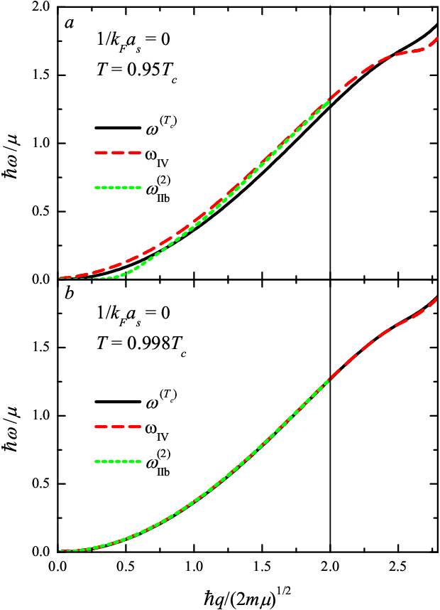
For completeness, we also show on Fig. 13 the poles found in window III (restricted to ) and IV. Both in frequency and damping and are close to the second pole of window II, (that is, as long as is much larger than ). Thus they also tend to when . In fact, they represent the same physical resonance: when , the pair-breaking continuum no longer exhibits the angular points , and (except for where coincides with ); this means that the analytic continuations through windows II to IV become simply equivalent.
At where only window IV remains, we note that lies above (thus fulfilling the piecewise rule and providing a sensible contribution to the pair field spectral function) in a wide range of values of . The eigenfrequency then shows a bump when it crosses the pair-breaking continuum edge. At very low , the solution is subsonic, as one of the solutions found by Ref. Castin at . However it develops the quadratic dispersion described in Sec. III.2 in the intermediate regime ().
IV.4 Visibility of the collective modes in spectral functions
Now that we have extracted the collective mode spectrum from the analytic continuations (both below (Sec. IV.2) and above (Sec. IV.3) the pair-breaking continuum), we study the manifestations of this spectrum in the spectral functions. Besides the pair response in the cartesian basis introduced in Eq. (17), we study here the modulus-modulus and phase-phase spectral functions:
| (27) | ||||
| (28) |
We note that , coincide when at fixed . Mathematically, this is because when can be neglected.
IV.4.1 Residues of the complex poles
Phononic branches
We first analyse the residues of different complex poles in and . Fig. 15.a shows the residues for the phonon-like branches and as functions of the relative temperature for a fixed momentum . The value of is chosen because it lies slightly below the exceptional-point value where the two poles undergo a head-on collision. Panel 15.a then illustrates the behavior of the residues near the exceptional point. The absolute values and of the residues of the two phononic modes show a resonant increase near (we checked numerically their divergence when ). However, because residues are complex and the phase of the residues are opposite at resonance, this does not result in a resonant enhancement of the spectral function when the temperature passes , as will be shown below in Fig. 16. The residues of the first and second modes remain close (in absolute value) in the whole considered interval of temperatures (both in the phase-phase and modulus-modulus channels). What determines the domination of over in the spectral functions at temperatures (and vice-versa the domination of over at ) is rather the crossing of the damping factors near (see panel 15.b).
The comparison of the phase and modulus residues also shows a clear domination of the phase channel (recall that in the long wavelength limit Klimin2019 one has ) except in the vicinity of where they converge to the same value, as expected.

Poles of window II
Panel c represents the residues of the two modes obtained using the analytic continuation through the window IIb: the pair-breaking “Higgs ” mode with the complex pole and the second mode of the same window, which tends to the pairing mode when . The eigenfrequencies and damping factors for these poles are shown in Fig. 15 d. This further illustrates how the pairing mode of Sec. III replaces the pair-breaking mode as approaches : in the cartesian spectral function , the residue of tends to 0 in the cartesian spectral function . Even in the modulus-modulus channel the residue of eventually dominates over that of . This effect adds up to a purely spectral effect (see panel d): the pair-breaking mode becomes overdamped near while the other mode exhibits the opposite trend, it is overdamped at lower temperatures, and its damping decreases when approaches .
IV.4.2 Analytic simulations of the spectral functions
We now wish to measure the amount of information on the spectral functions which is contained in the spectrum and residues found in the analytic continuation. For this, we define (as in Ref. Klimin2019) “analytic simulations” of the spectral functions using the poles and residues in each of the 5 continuation windows:
| (29) | ||||
| (30) |
where the index in a partial contribution indicates the interval used for the analytic continuation, and labels the complex poles of the GPF propagator continued through this interval. Here, are the angular-point frequencies as described above, completed by and and sorted in the ascending order as follows: , , , and . Particularly for , the interval between and shrinks to zero and does not contribute to . The Heaviside step function is used on the same reasoning as in Ref. Klimin2019: poles from an analytic continuation are relevant for the spectral function only in the interval through which the analytic continuation passed. It should be noted that the step function means the piecewise rule for the argument of the spectral function but not a piecewise rule for complex poles . For a fixed contribution , real parts of relevant poles may move beyond the interval , as discussed in the caption of Fig. 6.
In Fig. 16.a, b, c, the spectral function and its analytic simulation are shown for the same momentum as chosen in Fig. 15, for three temperatures: below, near and above the crossing-point temperature for damping factors. Also, partial contributions of different poles to are plotted. Fig. 16.d for and a larger wavevector () shows the spectral function and its analytic simulation when temperature moves closer to and the momentum is sufficiently large so that the resonance peak lies in the pair-breaking continuum. We note that since the residues are complex, the partial contributions to are not everywhere positive.

In all four panels of (16), we observe that the total analytic simulation is remarkably close to the spectral function . This indicates that the poles found in the analytic continuation are a good summary of the shape of the spectral function. When the frequency passes a bound between two neighboring intervals for the analytic continuation, the retained partial contributions abruptly change due to the Heaviside function in (29). In some cases, this leads to a well expressed discontinuity of at a “sharp” angular point, as on panels 16 a,b,c at . In other cases, the discontinuity of is much smaller than the average value of the function, such that the discontinuity at a “soft” angular point is hardly resolvable by eye. This happens either because two adjacent intervals have almost the same poles in their analytic continuation, and hence almost equal partial contributions (the case of panel 16 d at , and ), or, more subtly, because two partial contributions add up to almost the same value of , despite having an important discontinuity at the angular point (the case of panel 16 b at ). This distinction between the “sharp” angular point () and “soft” ones (, and ) has a physical origin: at the soft angular points only the configuration of resonant wavevectors changes, not the damping mechanism itself. On the contrary, separates regions where the damping channel by emission of broken pairs is either opened or closed. This being said, we note that the sharpness of decreases when at fixed (see panel 16 d). This is expected: at the quasiparticle-quasiparticle continuum is no longer distinguishable from the rest of the particle-hole continuum.
Having a comparable residue, the two phononic poles have overall comparable contributions. At the resonance of residues (Fig. 16 b) the two poles participate in the peak of almost equally. When , the broadening of the partial contribution of makes its contribution near the peak of comparatively smaller. It should be noted that the resonance of residues is not manifested in the temperature behavior of the total spectral function. Moreover, the change of a dominant partial contribution can hardly be distinguished in the total response, and can be extracted only using the analytic simulation.
When approaches (Fig. 16 d), the maximum of the pair field response enters the pair-breaking continuum. In windows IIa and IIb, the main peak almost entirely proceeds from , the contribution of the first pole (the pair-breaking “Higgs mode”) being negligible. The peak extends almost without discontinuity or angular points onto window III and IV. This does not surprises us since , and and all tend asymptotically to each other and to the pairing mode analyzed in Sec. III (recall Fig. 14). Near , the angular points separating those 4 intervals tend to disappear, which makes the analytic continuation through the 4 windows nearly equivalent. Although the discussion is purely formal since the intervals are equivalent, we note that the width of windows IIb and III tends to 0 as such that only intervals IIa and IV remain.

IV.4.3 Evolution of collective modes near
To better illustrate how the spectral function evolves from a phonon/Higgs mode regime at low temperature, to a regime dominated by the quadratic pairing mode, we show on Fig. 17 contour plots of the modulus-modulus and phase-phase spectral functions. On top of the contour plots, we indicate selected eigenfrequencies from roots of Eq.(3). Here, only the roots which give the most significant contributions to the spectral functions have been plotted66 6 Here, the choice between “a” and “b” windows needs an explanation. It depends on the fact whether the analytic simulation using this window is appropriate to reproduce the spectral function . More clearly, for , the “Higgs” mode lies above the angular-point frequency in the range of momenta where it is not overdamped. The sound-like mode frequencies at the same temperature are mainly lower than . Consequently, we plot here , , and , choosing the interval “a” for sound-like modes and “b” for modes in the continuum. Also, this explains a choice of representative intervals for the analytic continuation in Fig. 15. On the contrary, at , the angular-point frequency appears to be higher than in the range of where the mode is not overdamped. Therefore the window “a” is relevant for Fig. 17 (c, d).. As approaches , the region of energy-momentum where the influence of the phononic-like modes and pair-breaking mode shrinks to a small window and , corresponding to the region where the existence of condensed pairs still matters. Elsewhere, the spectral function is dominated by a resonance well summarized by (and the associated residue77 7 We note that and , the complex residue clearly shifts the peak of the resonance away from .). Fig. 17 thus illustrates the reduction of the phononic/pair-breaking regime when , and the corresponding growth of a regime dominated by the pairing collective mode . Again we note that and coincide when at fixed as is clearly visible on the lower panels of Fig. 17.
V Conclusions
We have investigated collective excitations in condensed Fermi gases in the whole range of the BCS-BEC crossover for finite temperatures below and beyond the small-momentum approximation. Eigenfrequencies and damping factors for different branches of collective excitations are calculated within the Gaussian pair fluctuation approach using a unified method of finding complex poles of the analytically continued GPF propagator. The real and imaginary parts of complex poles are calculated mutually consistently, beyond the perturbation theory for damping. This makes it possible to consider collective excitations also in cases when damping is not small.
At and near , we showed that a quadratically-dispersed collective mode, acting as a precursor of the phase transition, is observable in the response of the system to a driving pairing field. This mode was predicted by Andrianov and Popov in the BCS limit Andrianov1976 and appears in the dissipative time-dependent Ginzburg-Landau equation of Ref. deMelo1993. We computed analytically its effective mass and showed how it varies from purely imaginary values in the BCS limit to purely real in the BEC limit. Away from we computed (to leading order in ) the energy shift, which acts as a gap in the BEC regime and as an extra damping rate in the BCS limit. Last, we explained how the resonance disappears at large when it encounters the lower-edge of the pairing continuum.
We note that the drastic change in the dispersion of the collective modes is predicted here within GPF theory, which approximates the correlation length critical exponent to its BCS value , in a quantitative disagreement with the calculated value for the universality class of superfluid Fermi gases Wetterich2010; Dupuis2016 and with the result of the conformal bootstrap calculation Chester2020. Integrating this correction to the study of collective modes near the transition temperature would certainly make the prediction more accurate. This needs of course a calculation beyond the GPF approximation, which is not able to study the critical regime quantitatively. Our approach also assumes an infinite quasiparticle lifetime, which restricts us for the study of collective modes to the collisionless regime. Extending our analysis to the hydrodynamic regime, where excitations analogous to Carlson-Goldman modes are expected, will be an important step forward. This requires a precise estimate of the quasiparticle lifetime, which, in an ultracold Fermi gas weakly coupled to its environment, should be limited by intrinsic processes such as quasiparticle collisions.
Away from the limits and , our general study allows us to track the evolution of different branches of collective excitations, and to make clear genetic relations between them. Particularly, we show that the collective mode near the transition temperature is genetically distinct from both pair-breaking and phononic modes (whose visibility domain shrinks to a small window and near ) as it is caused by the appearance of new poles in the analytic continuation. At , eigenfrequencies and damping factors exhibit a nontrivial momentum and temperature dependence. Particularly, they can be non-monotonic as functions of . Moreover, different eigenfrequencies may cross each other and change their relative significance when varying momentum and temperature. The present study clarifies then some unexplored questions in the theory of collective excitations in superfluid Fermi gases. The applied method can be straightforwardly extended to more complicated condensed fermionic systems, e. g., multiband or color superfluids.
Appendix A Fluctuation matrix
We recall here the elements of the order-parameter fluctuation matrix in modulus-phase basis (for the matrix , in the cartesian basis see Eqs. (10) and (11) in Klimin2019).
| (31) |
| (32) |
| (33) |
| (34) |
where we use and is the BCS excitation energy, is the free-fermion energy, and is the function
| (35) |
These matrix elements coincide with those introduced in Refs. Engelbrecht.
Appendix B Details on the long wavelength calculation near
We give here more details on the calculation of the collective mode spectrum leading to expression (11) above and (13) below . Above , we add and subtract the sum to , leading to:
| (36) |
with
| (37) | |||||
| (38) |
Omitting terms of order , one can then approximate by its value in :
| (39) |
Below , one should take into account the non-vanishing off-diagonal matrix element as well as the deviation of the diagonal elements due to the non-zero value of the gap. We compute the latter quantity by setting before expanding for :
| (40) |
To recognize in the first sum of the right-hand-side of (40), we have used the gap equation in the form
| (41) |
For the second sum, we use the link between and obtained by expanding (41) for with :
| (42) |
We then approximate
| (43) |
To compute , we use the equality on the real axis before doing the analytic continuation
| (44) |
Finally, for the off-diagonal element , the value in , suffices to leading order in :
| (45) |
Acknowledgements.
We acknowledge financial support from the Research Foundation-Flanders (FWO-Vlaanderen) Grant No. G.0618.20.N, and from the research council of the University of Antwerp.References
- (1) G. C. Strinati, P. Pieri, G. Röpke, P. Schuck, and M. Urban, The BCS–BEC crossover: From ultra-cold Fermi gases to nuclear systems, Physics Reports 738, 1 (2018).
- (2) M. Yu. Kagan and A.V. Turlapov, BCS-BEC crossover, collective excitations and superfluid hydrodynamics in quantum fluids and gases, Physics-Uspekhi, 188, 225 (2019).
- (3) M. Bartenstein, A. Altmeyer, S. Riedl, S. Jochim, C. Chin, J. H. Denschlag, and R. Grimm, Collective Excitations of a Degenerate Gas at the BEC-BCS Crossover, Phys. Rev. Lett. 92, 203201 (2004).
- (4) J. Kinast, A. Turlapov, and J. E. Thomas, Damping of a Unitary Fermi Gas, Phys. Rev. Lett. 94, 170404 (2005).
- (5) A. Altmeyer, S. Riedl, C. Kohstall, M. J. Wright, R. Geursen, M. Bartenstein, C. Chin, J. Hecker Denschlag, and R. Grimm, Precision Measurements of Collective Oscillations in the BEC-BCS Crossover, Phys. Rev. Lett. 98, 040401 (2007).
- (6) M. K. Tey, L. A. Sidorenkov, E. R. S. Guajardo, R. Grimm, M. J. H. Ku, M. W. Zwierlein, Y.-H. Hou, L. Pitaevskii, and S. Stringari, Collective Modes in a Unitary Fermi Gas across the Superfluid Phase Transition, Phys. Rev. Lett. 110, 055303 (2013).
- (7) L. A. Sidorenkov, M. K. Tey, R. Grimm, Y.-H. Hou, L. Pitaevskii, and S. Stringari, Second sound and the superfluid fraction in a Fermi gas with resonant interactions, Nature (London) 498, 78 (2013).
- (8) S. Hoinka, P. Dyke, M. G. Lingham, J. J. Kinnunen, G. M. Bruun, and C. J. Vale, Goldstone mode and pair-breaking excitations in atomic Fermi superfluids, Nat. Phys. 13, 943 (2017).
- (9) C. C. N. Kuhn, S. Hoinka, I. Herrera, P. Dyke, J. J. Kinnunen, G. M. Bruun, and C. J. Vale, High-Frequency Sound in a Unitary Fermi Gas, Phys. Rev. Lett. 124, 150401 (2020).
- (10) R. Combescot, M. Yu. Kagan, and S. Stringari, Collective mode of homogeneous superfluid Fermi gases in the BEC-BCS crossover, Phys. Rev. A 74, 042717 (2006).
- (11) R. B. Diener, R. Sensarma, and M. Randeria, Quantum fluctuations in the superfluid state of the BCS-BEC crossover, Phys. Rev. A 77, 023626 (2008).
- (12) Y. Ohashi and A. Griffin, Superfluidity and collective modes in a uniform gas of Fermi atoms with a Feshbach resonance, Phys. Rev. A 67, 063612 (2003).
- (13) H. Kurkjian, Y. Castin, and A. Sinatra, Concavity of the collective excitation branch of a Fermi gas in the BEC-BCS crossover, Phys. Rev. A 93, 013623 (2016).
- (14) H. Kurkjian and J. Tempere, Absorption and emission of a collective excitation by a fermionic quasiparticle in a Fermi superfluid, New J. Phys. 19, 113045 (2017).
- (15) S. N. Klimin, J. Tempere, and H. Kurkjian, Phononic collective excitations in superfluid Fermi gases at nonzero temperatures, Phys. Rev. A 100, 063634 (2019).
- (16) J. R. Engelbrecht, M. Randeria, and C. A. R. Sá de Melo, BCS to Bose crossover: Broken-symmetry state, Phys. Rev. B 55, 15153 (1997).
- (17) H. Kurkjian, S. N. Klimin, J. Tempere, and Y. Castin, Pair-Breaking Collective Branch in BCS Superconductors and Superfluid Fermi Gases, Phys. Rev. Lett. 122, 093403 (2019).
- (18) H. Kurkjian, J. Tempere, and S. N. Klimin, Linear response of a superfluid Fermi gas inside its pair-breaking continuum, Sci. Rep. 10, 11591 (2020). https://doi.org/10.1038/s41598-020-65371-9.
- (19) Y. Castin and H. Kurkjian, Branche d’excitation collective du continuum dans les gaz de fermions condensés par paires: étude analytique et lois d’échelle,Comptes Rendus. Physique 21, 253 (2020).
- (20) C. A. R. Sá de Melo, M. Randeria, and J.R. Engelbrecht, Crossover from BCS to Bose superconductivity: Transition temperature and time-dependent Ginzburg-Landau theory, Phys. Rev. Lett. 71, 3202 (1993).
- (21) Philippe Nozières, Le problème à N corps: propriétés générales des gaz de fermions (Dunod, Paris, 1963).
- (22) V. A. Andrianov and V. N. Popov. Gidrodinamiceskoe dejstvie i Boze-spektr sverhtekucih Fermi-sistem. Teor. Mat. Fiz. 28, 341 (1976). [English translation: Theor. Math. Phys. 28, 829 (1976)].
- (23) P. Nozières and S. Schmitt-Rink, Bose condensation in an attractive fermion gas: From weak to strong coupling superconductivity, J. Low Temp. Phys. 59, 195 (1985).
- (24) R. V. Carlson and A. M. Goldman, Dynamics of the order parameter of superconducting aluminum films, J. Low Temp. Phys. 25, 67 (1976).
- (25) S. Diehl, S. Floerchinger, H. Gies, J. M. Pawlowkski, and C. Wetterich, Functional renormalization group approach to the BCS-BEC crossover, Annalen der Physik 522, 615 (2010).
- (26) T. Debelhoir and N. Dupuis, Critical region of the superfluid transition in the BCS-BEC crossover, Phys. Rev. A 93, 023642 (2016).
- (27) Shai M. Chester, Walter Landry, Junyu Liu, David Poland, David Simmons-Duffin, Ning Su, and Alessandro Vichi, Carving out OPE space and precise O(2) model critical exponents, J. High Energ. Phys. 2020, 142 (2020).