Risk-Averse RRT* Planning with Nonlinear Steering and Tracking Controllers for Nonlinear Robotic Systems Under Uncertainty
Abstract
We propose a two-phase risk-averse architecture for controlling stochastic nonlinear robotic systems. We present Risk-Averse Nonlinear Steering RRT* (RANS-RRT*) as an RRT* variant that incorporates nonlinear dynamics by solving a nonlinear program (NLP) and accounts for risk by approximating the state distribution and performing a distributionally robust (DR) collision check to promote safe planning. The generated plan is used as a reference for a low-level tracking controller. We demonstrate three controllers: finite horizon linear quadratic regulator (LQR) with linearized dynamics around the reference trajectory, LQR with robustness-promoting multiplicative noise terms, and a nonlinear model predictive control law (NMPC). We demonstrate the effectiveness of our algorithm using unicycle dynamics under heavy-tailed Laplace process noise in a cluttered environment.
Supplementary Material
Code supporting this project is available at https://github.com/TSummersLab/RANS-RRTStar.
I Introduction
Safe deployment of mobile robots in uncertain dynamic environments, such as urban streets and crowded airspaces, requires a systematic accounting of various risks, both within and across layers in an autonomy stack. These autonomy stacks are naturally partitioned into a hierarchy of i) a high-level planner which generates a reference trajectory (often) offline before system operation, and ii) a low-level controller whose purpose is to track the reference trajectory in an online fashion and incorporate feedback to mitigate the effect of disturbances. The survey [12] examines several approaches for motion planning and control of autonomous ground vehicles and suggests two additional upper layers in the hierarchy, namely route planning and behavioral decision-making. In this paper, we assume such route plans and behavioral decisions are encapsulated by the motion planning and control problems.
Many motion planning algorithms have been developed under deterministic settings and assume linear robot dynamics in order to simplify their analysis and design. However, in practice, robotic systems are inherently both nonlinear and stochastic in nature due to external disturbances and noisy onboard sensors. In the presence of model uncertainty or process noise, the resulting trajectory is only a nominal reference and there are no guarantees of its safety. To account for the stochastic components and to provide probabilistic guarantees, motion planning under uncertainty has been considered in several lines of recent research [2, 17]. Specifically, risk-aware motion planning algorithms for linear robot dynamics were developed recently using CVaR- [6] and Wasserstein metric- [8] based formulations.
A chance-constrained version of RRT and RRT* respectively were proposed in [9, 10], where chance constraints were used to encode the risk of constraint violation to provide probabilistic feasibility guarantees for robots with linear dynamics under additive uncertainties. On the other hand, these approaches made questionable assumptions of Gaussianity for system uncertainties ostensibly to maintain computational tractability. It was shown in [15] that such assumptions can lead to significant miscalculations of risk, and hence moment-based ambiguity sets were formulated to propose a distributionally robust variant of RRT called DR-RRT. This approach was extended in [13] to design an asymptotically optimal RRT* using output feedback with linear quadratic regulator and Kalman filter-based state estimation. Here we take a first step towards designing risk-aware nonlinear steering-based motion plans for nonlinear robotic systems. This is closely aligned with the problem addressed by authors in [7]. A low-level tracking controller is implemented to successfully track a given reference trajectory in the presence of uncertain process disturbances. In this work, we assume perfect state estimates are available and consider full-state feedback controllers. The linear-quadratic regulator (LQR) controller being the most common can be obtained through dynamic programming where a quadratic cost involving state deviation and control effort is minimized. The LQR controller can further be generalized to achieve robust stability under parametric model uncertainties by designing it to mean-square stabilize the system with the inclusion of multiplicative noises as described in [5] (LQRm). However, both LQR controllers cannot handle state and input constraints. On the other hand, NMPC explicitly considers both state and input constraints [11]. The authors in [4] used the nonlinear model-predictive control (NMPC) to track the LQR-RRT* trajectory to make up for linearization error. By contrast, we use NMPC to track a risk-averse RRT* trajectory generated by a nonlinear program (NLP)-based steering function which much more closely resembles the low-level NMPC controller.
Contributions:
- 1.
We present RANS-RRT*, a new sampling-based motion planner for nonlinear robotic systems which constructs dynamically feasible trajectories that satisfy distributionally robust state constraints to promote safety.
- 2.
We demonstrate our proposed approach on unicycle dynamics under heavy-tailed Laplace process noise in a cluttered environment. We provide a comparative study of the collision-avoidance rate, state deviation and control costs, and computational expense of three low-level reference tracking controllers i) LQR, ii) LQRm and iii) NMPC, across a range of disturbance strengths, through Monte Carlo simulations.
The rest of the paper is organized as follows. The notation, preliminaries and problem formulations are presented in §Notations, Preliminaries & Problem Formulation. The proposed nonlinear dynamics-based high level motion planner is elucidated in §II. Low-level tracking controllers are described in §III. Simulation results are reported and analyzed in §IV. Finally, the paper is closed in §V along with directions for future research.
Notations, Preliminaries & Problem Formulation
The set of real numbers and natural numbers are denoted by respectively. The subset of natural numbers between with is denoted by . The operator denotes set subtraction and denotes the cardinality of the set . An identity matrix in dimension is denoted by . The operator denotes the set complement.
I-A Environment and Obstacles Specification
Consider a robot in an environment with static obstacles. It is expected to navigate the environment while safely avoiding obstacles at all times. We denote the set of all obstacles by with . The environment and obstacles (assumed disjoint) are convex polytopes and hence can each be represented as a conjunction of halfspace constraints. The space occupied by the obstacle in is denoted . The union of the space occupied by all obstacles is . Hence the free space in the environment is given by
For a given deterministic state , the condition for collision avoidance with all obstacles is
where each individual obstacle avoidance constraint can be expressed as
and the condition for collision avoidance with the environment bounds is
where are the number of constraints for obstacle and are those of the environment. The total number of constraints is denoted .
I-B Robot System Dynamics
For all time instances , we model the robot as a discrete-time nonlinear dynamical system given by:
| (1) |
where are the system state, additive disturbance, and control input, respectively, at the time step indexed in the brackets, is the initial state, and is the robot dynamics that represents the nonlinear transformation. The disturbances are assumed independent and identically distributed according to some prescribed distribution .
I-C Unscented Transformation and Moment Estimation
The unscented transformation (UT) can be used to estimate the statistics of a random variable which undergoes a nonlinear transformation. An ensemble of samples called sigma points are generated deterministically [16] and propagated individually through the nonlinear transformation to yield an ensemble of transformed sigma points. The weighted statistics of the transformed sigma points approximate the statistics of the transformed random variable. Though parameters that generate the sigma points can be tailored for specific distributions, there is no pre-defined set of rules that work in general for all distributions. For a discrete-time nonlinear robot system as in (1), we can use the UT to estimate the mean and covariance of the next state given the current one. To do so, the ensemble of sigma points are obtained as follows
where is the row or column of the matrix obtained through Cholesky decomposition. Then, the weights below are used to scale in the estimation of the mean and covariance
| (2) | ||||
is a scaling parameter where are used to tune the unscented transformation. Usually is a good choice for Gaussian uncertainties, is a good choice for , and is an appropriate choice for , where a larger value for spreads the sigma points further from the mean. Using the above-obtained sigma points and the weights defined in (2), the estimated mean and covariance of the random variable under the dynamics (1), assuming Gaussian noise , are computed as follows.
I-D Moment-Based Ambiguity Set for The State Distribution
The state is a random vector. The state , under input and the noise , evolves to . Due to the difficulty in estimating the distribution of a random variable under a nonlinear transformation, we will assume that a state belongs to an unknown distribution . Since we can estimate its first two moments, we can consider a moment-based ambiguity set with the estimated moments. This will guarantee robustness to errors in propagating the state distribution due to the nonlinear dynamics. It can also provide robustness to moment estimation errors. The mean and covariance we consider for the ambiguity set are the ones we estimate through the UT and thus we get the following estimate for the ambiguity set:
For Gaussian inputs, the above moment estimates from UT are accurate up to the third-order approximation and for the case of non-Gaussian, the approximations are accurate to at least the second-order as described in [16].
I-E Nonlinear Motion Planning Problem
The planning problem provides a high-level solution that can then be used by low-level tracking controllers. This plan can be computed offline and requires finding an optimal reference trajectory that satisfies the robot dynamics, state and input constraints, and risk constraints. In this work, we consider the following planning problem.
Definition 1 (Optimal Risk-Based Path Planning Problem).
Given an initial state and a set of final goal locations , find a measurable state-and-input-history-dependent control policy with that minimizes the finite-horizon additive cost function subject to constraints:
| (3) | ||||
| s.t. | (1) | |||
| (4) | ||||
| (5) | ||||
| (6) | ||||
| (7) |
Here, is a stage cost function, (5) is the inputs constraint, (6) is the states risk constraint that ensures that the state, under the worst-case distribution, is in the free space with high probability specified through the stage risk bound , and (7) is the goal constraint requiring the final state to be in the goal region.
Remark 1.
The risk constraint (6) is infinite dimensional and generally non-convex which makes solving this problem a challenge.
To understand the stage risk constraints (6) in the context of trajectory safety, let denote the event that plan succeeds and be the complementary event (i.e. failure). Consider the specification that a plan succeeds with high probability or equivalently that it fails with low probability . Failure requires at least one stage risk constraints to be violated. Using the fact that
and applying Boole’s law, the probability of the success event can be lower bounded as follows:
If the stage risks are equal, meaning , then . Furthermore, if the stage risk is equally distributed over all constraints, then, the risk bound for a single constraint is and the risk bound for a single obstacle (or the environment ) is (or ) (this will be discussed more in §II-C).
Remark 2.
In general, may not be known ahead of time. For sampling-based planners, depends on the random nodes sampled. In such cases, an upper bound can be used . The choices of , the risk bound on the plan’s failure , and the risk budget allocation across time steps and constraints are design parameters. Alternatively, it is also possible to build up the risk bounds from the individual constraints into a risk bound on the whole plan [14].
I-F Nonlinear Reference Trajectory Tracking Problem
Given a reference trajectory for generated by the high-level motion planner, the reference tracking problem involves minimizing deviations of the state from the reference state subject to the nonlinear dynamics and realizations of all system uncertainties. This problem is formally presented below.
Definition 2 (Optimal reference trajectory tracking problem).
Given reference trajectory for such that and , find a measurable state-and-input-history-dependent control policy with that minimizes the finite-horizon additive cost function subject to constraints:
| s.t. |
where is a stage cost function that penalizes the control effort and deviations of the robot state from those of the reference trajectory at each time step.
II High Level Planner: RANS-RRT*
The high-level planner finds an optimal (or approximately optimal) plan for the low-level controller to execute. If the plan gets close to obstacles, tracking might fail due to process noise. By incorporating uncertainty in the high-level planner, a more conservative, but safe, trajectory is designed. In this work, we present an approximate solution to the problem in Definition 1 using rapidly exploring random trees. We propose RANS-RRT*: a Risk-Averse, Nonlinear Steering RRT* planner. Below, we discuss: 1) the NLP problem used to steer between tree nodes, 2) the mean and covariance propagation along such a trajectory segment, 3) the treatment of uncertainty and risk, 4) the RANS-RRT* algorithm, and 5) a trajectory shortening post-processing step.
II-A NLP Steering
Our RANS-RRT* algorithm employs a nonlinear steering law to compute a trajectory of length consisting of state and input pairs that drive an initial state to a final one . The first state belongs to the RANS-RRT* tree and the other is either a sampled state or another tree state. NLP steering is defined below.
Definition 3 (NLP Steering).
Given an initial state , a desired state , and a steering horizon , the NLP steering solution is the set of states and controls to the following deterministic optimization problem without any risk constraints.
| (8) | ||||
| s.t | ||||
II-B Mean and Covariance Propagation
NLP steering returns the trajectory . To use this in the RANS-RRT* tree , as a trajectory between two nodes, we need the mean state, covariance of the state, and control law. Since the dynamics are nonlinear and the NMPC control policy is the solution of a constrained optimization problem without an explicit form as a function of the state, it is extremely challenging to incorporate the NMPC feedback law into the RANS-RRT* trajectories. As such, we use the open-loop controls of the NLP trajectory . As a byproduct, we also require the mean states in the RANS-RRT* trajectory to match the states of the NLP trajectory . With the mean states and inputs fixed according to , we only need to estimate the covariance at the mean states. To do so, we use the UT with the NLP controls and match the UT mean states with the NLP states. This returns covariances associated with every state that are used in enforcing risk bounds. Thus, for every computed NLP trajectory we obtain a RANS-RRT* trajectory of the form where and for all .
II-C Risk Treatment
Consider a mean state and covariance pair in the RANS-RRT* trajectories . The risk constraint associate with this time step has the form
Since is a union of the obstacle sets, we use Boole’s law to get:
We allocate the risk bound equally among the constraints by setting the risk bound for being in to and that of not being in the environment to . Thus:
and hence, the desired risk constraint is enforced. Now we turn our attention to satisfying:
| (9) | ||||
| (10) |
As for (10), we have the following:
and
| (11) |
where (11) follows from the Fréchet-Boole lower bound. We then have the following result:
which holds as , i.e. by enforcing the left-hand-side, the right-hand-side (desired constraint) is guaranteed. Therefore, (6) is satisfied if
Using [3, Theorem 3.1] these are equivalent to:
| (12) | ||||
| (13) |
II-D Algorithm
RANS-RRT* is presented in Algorithm 1. The free space is first sampled and the tree is initialized with the initial state (the root of the tree) and the initial covariance of zero (lines 1-1). Then the sampled states are traversed. For every state , the nearest node in the tree is found (line 1). If the distance between and is larger than some threshold, a closer state is returned along the same direction (line 1). In line 1, NLP steering is performed to find a trajectory from to within the steering horizon . If steering fails, the sample is skipped. Else, a RANS-RRT* trajectory (mean states, covariances, and inputs) is returned. In line 1, the trajectory is checked for collisions. A collision is detected if any of the risk-tightened constraints ((12), (13)) are violated at any of the mean states, in which case the sample is skipped. If safe, the trajectory may be added to the tree after checking nearby nodes for a more optimal trajectory as done in RRT* (line 1). Then, the trajectory is added to the tree (line 1) and undergoes the RRT* rewiring set (line 1). Note that the rewire step also uses the same steering and collision check functions described before. When an optimal trajectory is queried, the trajectory with the smallest total NLP steering cost (output cost of Definition 3) is returned.
Remark 3.
RANS-RRT* only approximately solves the problem in Definition 1 because 1) the risk treatment step approximately solves the infinite-dimensional constraint (6), 2) the covariance estimation step using UT is imperfect for non-Gaussian distributions, and 3) the covariance propagation assumes the estimated means and NLP means coincide, which is used to keep the problem tractable. Hence, we do not make any formal risk-bound guarantees. Nonetheless, as we will see in the experimental results section, the padding added to obstacles through the DR collision check step makes the algorithm significantly robust to disturbances.
II-E Post-Processing: Trajectory Shortening
In the RANS-RRT* algorithm, the horizon used for solving the NLP steering problem is fixed. This is done to obtaining a decision on whether a trajectory exists between two nodes after solving one NLP problem. Ideally, we would want to solve the NLP steering problem with the shortest steering horizon. However, this is not trivial and might involve solving the steering problem with an increasing horizon after each failure (up to a certain upper bound). Since the NLP steering problem is computationally expensive, repeating the process would quickly make the problem intractable. To that end, we set the NLP steering horizon to a constant value during RANS-RRT* but perform a post-processing trajectory-shortening step to the optimal trajectory.
The post-processing step considers each trajectory between two RANS-RRT* nodes and obtains a new NLP steering trajectory by solving the problem in Definition 3 for a different steering horizon . is initially set to a small estimated value (which we assign based on the trajectory length and the robot dynamics). If NLP steering fails, is incremented and the process is repeated while (at which point the original trajectory is used). If a trajectory is found, the same covariance propagation and DR collision-avoidance steps as done in RANS-RRT* are performed. If the DR checks fail, is incremented and the process continues. If they succeed, the RANS-RRT* trajectory is updated with the shorter one.
We observed significantly shorter trajectories after performing this step. Furthermore, since the trajectory time is fixed based on the trajectory steering horizon ( where is the discrete-time step), RANS-RRT* trajectories have fixed duration regardless of the distance between nodes (causing slow and fast trajectories) whereas the shortened trajectories have different times leading to smoother trajectories.
III Tracking Controllers
The low-level problem in Definition 2 was specified as the evaluation criterion of performance of the tracking controllers. However, our tracking controllers do not exactly solve the low-level problem in Definition 2, but instead approximately solve it using established control design methodologies. Compared with Definition 2, the proposed tracking controllers make the following approximations. The LQR and LQRm controllers assume dynamics are linearized about the reference trajectory (so (1) only holds approximately), and the input constraint (5) is ignored. LQRm attempts to mitigate the effects of linearization error by treating the model errors as multiplicative noise. NMPC solves an optimal control problem more similar to the one in Definition 2, but the finite horizon is generally shorter and the effect of the process noise (4) is ignored by replacing the stochastic dynamics (1) with their expectation. Furthermore, we chose to add a state constraint that requires the nominal state to be in the environment . Details of the control design techniques are given throughout the remainder of this section for completeness.
In all low-level controllers we use identical low-level cost functions. This facilitates a fair comparison between controllers, as the same objective is approximately optimized. We use stage costs which are quadratic in the state deviation and input:
where and the penalty matrices and are symmetric positive definite for all .
III-A Robot dynamics
We consider the problem of navigating a robot with unicycle dynamics from an initial state to a final set of states. The discrete-time unicycle nonlinear dynamics obtained through forward-Euler discretization of the corresponding continuous-time dynamics are given by:
| (14) | ||||
where are the horizontal and vertical positions of the robot, is the heading of the robot relative to the -axis of an assigned world frame, are the linear and angular velocity control inputs, and are the disturbances affecting each state, all expressed at timestamp . The quantity is the sampling time in seconds between any two timestamps . With short-hand notations
the dynamics in (III-A) and corresponding Jacobians can be written in the compact form as
III-B Generalized linear-quadratic control
In this subsection we propose and derive the solution to a generalized linear-quadratic control problem (LQP), which will be useful in the sequel. Consider the following finite-horizon stochastic dynamic game:
| (15) | ||||
| subject to |
with linear dynamics and quadratic stage costs
where
where the expectation is with respect to the random variables
which are distributed as
where is any distribution with mean zero and covariance , and the random variables are assumed statistically independent. The variables have the following meanings: is the state, is a control input, is an adversarial input, is an exogenous signal, and is a disturbance. This formulation allows the policies to be shaped by the exogenous signal and its interaction with the state and inputs and ; specifically, in the sequel we will choose to be the concatenated reference state and input trajectory. The stochastic system matrices , , and are decomposed into the mean system matrices , , and and multiplicative noise terms, which are further decomposed into the pattern matrices , , and the scalar mutually independent random variables , , which are distributed according to distributions , , which have mean zero and variances , , . The matrices specify how the additive disturbance enters the dynamics. The matrices are assumed to satisfy block semidefiniteness conditions that make the stage costs convex in the state , control input , and exogenous signal , and concave in the adversarial input . The matrices specify quadratic cost weights for each state, control input, adversarial input, and exogenous signal. Notice that the stage costs and dynamics in the LQP are different from those used in the high-level planner, i.e. and .
Optimal policies can be computed from optimal cost functions via dynamic programming backwards in time. The initial cost function is
where
i.e. a convex quadratic polynomial of . The subsequent cost functions are found via the dynamic programming equation:
where is the state-action cost function
where expectation is with respect to . We will show that if the current cost function is quadratic in , i.e. has the form
then the prior cost function is also quadratic in , i.e.
and we will provide the explicit relation between , , and , , , which will also be needed to compute the optimal policies. Then, arguing by induction and noting that by assumption the terminal cost function is quadratic in , all cost functions until are quadratic in with the same form.
We begin by evaluating the state-action cost function using the assumption that is quadratic in :
To ease notation, for the following development we will drop the indices and , so
where the last step follows by the zero mean and independence assumptions on the relevant random variables. Since is convex in , the minimum with respect to is found when the gradient with respect to is equal to 0:
rearranging,
| (16) |
Likewise, since is concave in , the maximum with respect to is found when the gradient with respect to is equal to 0:
rearranging
| (17) |
Rewrite the expressions for and as
| (18) | ||||
| (19) |
where
Now we decouple the expressions for and . First substitute (19) into (18) to obtain
rearranging
rearranging
where the gains are defined as
An analogous calculation for yields
where the gains are defined as
Substituting the optimal input into the state-action cost function, we obtain the optimal cost function
Grouping terms in quadratic, linear, and constant quantities of the state, we find indeed that is a convex quadratic of the state, i.e.
with
Notice that the control policies do not depend on the scalar part of the cost or the noise covariance , so it is not strictly necessary to compute or require specification of , for the purpose of control.
| Dynamics matrix sequences | , , , |
| Multiplicative noise pattern matrices | , , |
| Multiplicative noise variances | , , |
| Additive noise covariance matrix sequence | |
| Penalty matrix sequence | |
| Exogenous signal |
At runtime, the solution from Algorithm 2 is used to generate control inputs at each time according to
Notice that these control actions are the summation of a state-feedback term and a feedforward term which can be computed before running the system. Notice also that the adversary gains , , are not needed explicitly, but rather promote robustness of the controller implicitly via their effect on the control gains , , .
III-C Tracking with Linear Controller
In order to apply optimal linear control, we linearize the discrete-time nonlinear dynamics about various operating points in the joint state-input space. From this section on, we notate . A first-order Taylor series approximation of evaluated at the operating point () is
The low-level controller receives a reference trajectory, a sequence of states, inputs and disturbances, from the high-level planner, denoted as . The low-level controller will use these as the operating points about which to linearize the dynamics, i.e. will assume the dynamics
| (20) |
We will also assume that the reference trajectory satisfies the nonlinear dynamics constraint, i.e.
Using this assumption, the dynamics in (20) simplify to
Defining the state-, input-, and disturbance-deviation variables
the dynamics in (20) can be rewritten as
| (21) |
with
which is clearly seen as linear time-varying dynamics in the deviation variables.
We now define general stage costs which are quadratic in the state, input, deviation of state from reference state, and deviation of input from reference input:
| (22) |
where are positive semidefinite matrices which penalize deviation of the state and input from the origin and are positive semidefinite matrices which penalize the deviation of the state and input from the reference. We provide equations in this level of generality, but practically the most meaningful thing to do is set and ; the former because keeping the robot near the (absolute) origin in state-space is contrary to our goals, and the latter because we really only care about the total control effort expended, which can be smaller than that used by the reference open-loop input sequence in the event that serendipitous disturbance realizations drive the robot towards the reference states “for free.” Choosing the particular values for and is a somewhat subjective task, but we will use diagonal and time-invariant matrices with “reasonable” values chosen that empirically give a good balance between reference tracking and control effort. We also make the assumption that the disturbance-deviations are independent, zero-mean and have covariance , i.e.
| (23) |
Using the linearized dynamics in (21), the time-additive quadratic stage-costs in (22), and the disturbance distribution assumption in (23), we obtain the linear-quadratic optimal tracking problem
| minimize | |||
| subject to | |||
We now show how to bring this tracking problem into the form of the generalized linear quadratic problem in (15). First, it is clear that the dynamics and disturbance distribution have the required form already. Next, rewrite the state and input in terms of the deviations and references as
so the stage cost can be expressed as
Treating the concatenated reference state and input trajectory as an exogenous signal, i.e.
the stage cost can be expressed as
where
At this point we re-introduce the additional terms which promote robustness of the linearized controller, as discussed in Section III-B. We assume an additive adversary disturbance affects the state-deviation dynamics directly, as well as state-deviation- and input-deviation- and adversary-input-multiplicative noises. We will only consider a quadratic penalty on the adversary input characterized by symmetric positive definite matrix . Thus, the robustified linear-quadratic tracking problem becomes
| minimize | |||
| subject to | |||
where
where
which matches the required form of the stage costs in (15). Thus, we can apply Algorithm 2 to compute the optimal policies. At runtime, the control inputs are computed as
which can again be interpreted as the summation of a closed-loop feedback term of the state-deviation and an open-loop feedforward term. As long as the state of the system remains close to the reference trajectory, the linearized dynamics will remain a good approximation and the linear controller will yield good reference tracking.
III-D LQR
For vanilla LQR, we do not include any robustness-inducing terms, i.e. set and .
III-E Robust LQR
We seek to promote robustness against errors in the state-space matrices due to linearization about states other than the reference trajectory, which occurs due to the process disturbance. Observing the Jacobians, only mis-specifications in heading change the entries. We assume that the heading deviation from reference is uniformly upper bounded as
For the unicycle model, it is straightforward to construct appropriate 2D bounding boxes in the space of A and B matrices that fully contain every possible Jacobian. Consider the - and -entries of the matrix
Through trigonometric relations depicted by Figure 1, we obtain the robustness regions
determined by directions
where and where the scales are bounded as
where

Note that the robustness region is conservative as it extends in the and directions twice as far as strictly necessary. This is done merely as a matter of convenience so that the center of the robustness region remains at (, ) regardless of . It has been proved in [5] that, in the infinite-horizon time-invariant setting, the inclusion of (fictitious) multiplicative noise in the control design induces robustness to static model perturbations in the same directions as the multiplicative noise. This inspires the inclusion of such multiplicative noises with variance and directions related to the desired robustness region over which we desire to minimize quadratic cost. We include the robust LQR in our comparison to demonstrate the benefit of our NMPC controller over a simpler robust control method.
III-F NMPC
NMPC can be used to approximate the nonlinear optimal trajectory tracking problem. NMPC accomplishes that by reducing the problem into a sequence of open-loop optimization problems over a horizon where after solving an NLP to track a reference trajectory, only the first input is applied and the horizon is shifted back. The NMPC tracking NLP is given below.
Definition 4 (NMPC Tracking NLP).
Given an reference trajectory for and a planning horizon , find a control sequence at time step that minimizes the -horizon additive cost function subject to constraints:
| (5) | |||
After solving this problem at step , only the first input is applied and the horizon is shifted to for the problem to be solved again. The final set of control inputs is thus .
IV Numerical Results
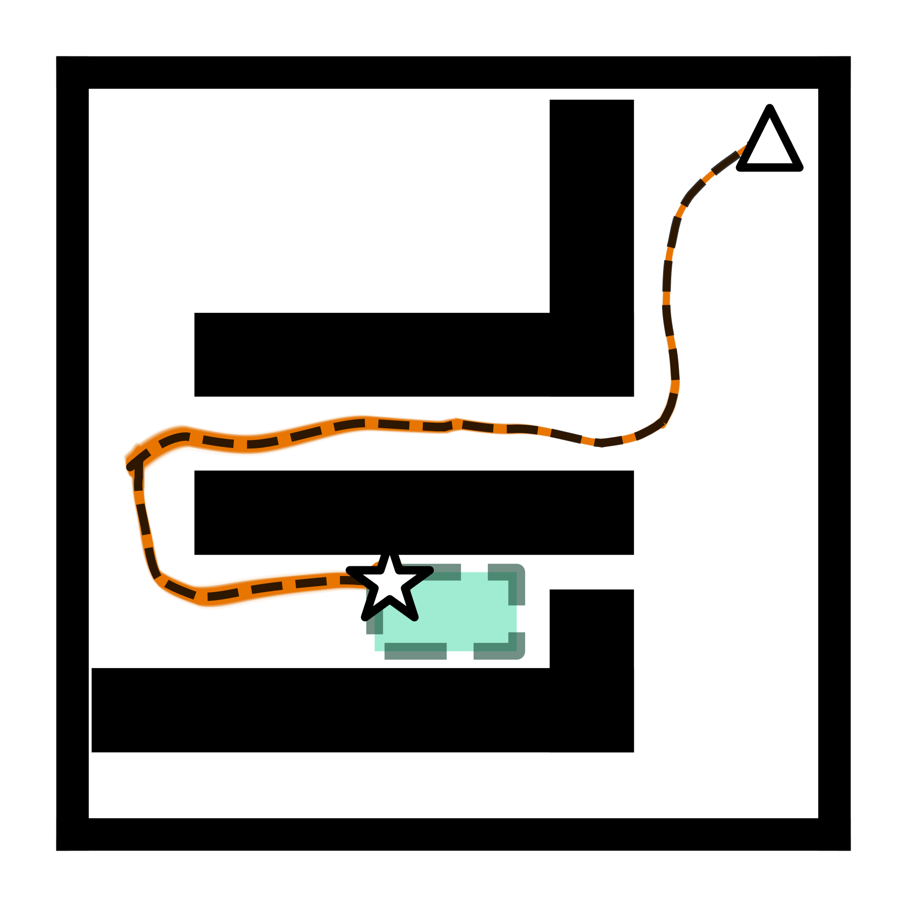
RANS-RRT* plans were generated on a machine with an Intel Core i7 6700K CPU and 16 of RAM. The low-level Monte Carlo simulations were performed on a machine with a Ryzen 7 2700X and 64GB of RAM. The NLP is modeled with CasADi Opti and solved with IPOPT [1]. We showcase RANS-RRT* in action in three different environments. Each environment consisted of a root node (white triangle), a goal area (dashed green rectangle), and a environment with 4 rectangular obstacles for its sides (black boundary). Environments 1 and 3 (Figures 4(a) and 4(c)) have 5 rectangular obstacles (black rectangles) while environment 2 (Figure 4(b)) has only 3 such obstacles. The robot is assumed to occupy a single point. Its controls bounds are units/sec for linear velocity and rad/sec for angular velocity. The RANS-RRT* steering horizon is and the NMPC planning horizon is . The discrete-time step was sec. The planner control cost matrix was . The tracking (LQR, robust LQR, and NMPC) cost matrices were and for all , and .
We used a high-level plan risk bound of . It is divided equally across the time steps and among the obstacle constraints. The process noise distribution was taken as a multivariate Laplace distribution with zero mean and covariance . The same variance was used for all states and is denoted by . We also refer to this as the noise level. In the tracking step, we evaluated performance under different (greater) noise levels.
IV-A RANS-RRT* Results
Constructing the RANS-RRT* trees in Figures 4(a)-4(c) took 36, 23, and 28 minutes respectively. Each tree started with randomly sampled nodes but only , , and nodes were deemed feasible and safe and added to the trees, respectively. The RANS-RRT* trajectories were conservative in the sense that they avoided getting too close to obstacles. Small gaps, such as to the right of the goal in Figure 4(c) or on the right side of the environment in Figure 4(b), were implicitly deemed too risky and avoided. On the other hand, a tree grown using the standard RRT* in the same environment in Figure 4(d) discovered such risky gaps and thereby returned an unsafe (risky) trajectory. In fact, it is easy to see that the optimal path to the goal in Figure 4(d) scrapes by an obstacle and hence would result in a collisions even for small process noise.
IV-B Low-Level Tracking Results
We used open-loop control and three low-level closed-loop controllers 1) LQR, 2) robust LQR, and 3) NMPC, to track a high-level trajectory in the environment shown in Figure 4(c) under realization of the Laplace noise. For each noise level, Monte Carlo simulations were performed. The resulting trajectories are plotted in Figure 2. As expected, the noise level assumed for the high-level plan was insignificant: even open-loop control succeeded. However, as the noise level increased, open-loop control began to fail. At around , the open-loop control almost always failed, while the other controllers almost always succeeded. From there, the feedback controllers began failing more frequently. Robust LQR did slightly better than LQR with fewer collisions for each noise level. Both were outperformed by NMPC which was better able to reject the more aggressive noise, leading to notably fewer collisions. The largest noise levels tested for which the plan failure risk bound of percent was satisfied were for LQR and robust LQR and for NMPC. These are, respectively, and folds larger than the assumed noise covariance .
For comparison, we ran the same experiment, but with the distributionally robust obstacle padding disabled. The planner returned trajectories which passed near obstacle boundaries, as shown in the tree in Figure 4(d), with realized trajectories plotted in Figures 8 and 7. Consequently, the reference trajectory itself was extremely unsafe, as evidenced by the high failure rates exhibited in Figure 3. Only at an extremely low noise level was NMPC able to reliably avoid collisions, while the LQR and LQRm controllers failed to do so. However with slightly more noise at the level , all control schemes led to significant probability of collision (greater than ). By contrast, the RANS-RRT* reference trajectory was so safe that even open-loop control led to a low probability of collision (less than ) at this noise level . This trend continued all the way up through the noise level with the probability of collision along the non-robust reference trajectory continuing to degrade, while the robust reference trajectory remained nearly perfectly safe with any of the low-level feedback controllers, thus demonstrating the clear benefit of RANS-RRT* over vanilla RRT*. Eventually the noise became too powerful and collisions became a near certainty regardless of the planner or controller used.
In Figure 6 the realized trajectories obtained through the Monte Carlo simulations are plotted for . The performance metrics for and are tabulated in Tables I and II respectively. We use the following metrics to evaluate the effectiveness of each tracking controller:
- 1.
The number of collisions: the number of Monte Carlo trials in which the realized trajectory collided with an obstacle.
- 2.
The average and costs: the realized state-deviation cost and control cost , conditionally averaged across all collision-free trajectories.
- 3.
The average run time: the time taken to run the entire Monte Carlo trial, conditionally averaged across all collision-free trajectories, which is necessary as simulations terminate immediately upon collision.
With , the trajectory was short enough so that collisions did not occur even with purely open-loop control, although the trajectories began to diverge from the reference. The closed-loop controllers exhibited minimal state deviations, as reflected in the significantly lower average cost. The difference in and costs between each closed-loop controller was insignificant; since the state remained extremely close to the reference, the inputs generated by each controller were very similar.
However with as shown in Figure 6, the following observations were made. Almost all open-loop trajectories ended with collisions as shown in Figure 6(a). Compared to the standard LQR, robust LQR led to a lower number of collisions and state-deviation cost as shown in Figures 6(b), 6(c) but both were significantly outperformed by NMPC. NMPC trajectories generally remained closer to the reference than LQR or robust LQR along with lower number of collision as the robot moved through the corridor as shown in Figure 6(d). However, NMPC’s closer reference tracking and collision-avoidance came at a price, as it used more control effort than LQR and robust LQR. Likewise, the more sophisticated computations involved in solving the NLPs in NMPC led to a longer average run time. It is evident that under both the noise settings, the NMPC outperforms other controllers in tracking the given reference trajectory to reach the goal with low failure rate and a better cost.
| Controller | Num. collisions | cost | cost | Run time (s) |
| Open-loop | 0 | 30.869 | 54.989 | 0.0103 |
| LQR | 0 | 3.403 | 43.267 | 0.1867 |
| LQRm | 0 | 2.911 | 44.351 | 0.2833 |
| NMPC | 0 | 3.522 | 43.240 | 5.6234 |
| Controller | Num. collisions | cost | cost | Run time (s) |
| Open-loop | 999 | 5103.148 | 54.989 | 0.0018 |
| LQR | 160 | 827.949 | 110.016 | 0.1751 |
| LQRm | 138 | 820.916 | 114.646 | 0.2946 |
| NMPC | 75 | 732.646 | 131.059 | 6.9159 |
V Conclusion and Future Work
We proposed a risk-averse control architecture tailored for safely controlling stochastic nonlinear robotic systems, which combines a novel nonlinear steering-based variant of RRT* called RANS-RRT* that accounts for risk by performing DR collision checks with low-level reference tracking controllers. We performed thorough numerical experiments using unicycle dynamics, compared three controllers, and observed better performance from NMPC than LQR variants. We showed that the despite the usage of very small noise level assumptions in the high-level planner, the low-level controllers performed well under moderate and aggressive disturbance realizations. Future research involves considering a full nonlinear sensor model while incorporating the exact DR risk constraints in the optimization problems of both the levels of autonomy stack for accurate risk assessment. We will also seek to decrease the computation time of NMPC through the usage of code generation tools.
References
- [1] J. A. E. Andersson, J. Gillis, G. Horn, J. B. Rawlings, and M. Diehl, “CasADi – A software framework for nonlinear optimization and optimal control,” Mathematical Programming Computation, vol. 11, no. 1, pp. 1–36, 2019.
- [2] L. Blackmore, M. Ono, and B. C. Williams, “Chance-constrained optimal path planning with obstacles,” IEEE Transactions on Robotics, vol. 27, no. 6, pp. 1080–1094, 2011.
- [3] G. C. Calafiore and L. El Ghaoui, “On distributionally robust chance-constrained linear programs,” Journal of Optimization Theory and Applications, vol. 130, no. 1, pp. 1–22, 2006.
- [4] B. Doerr and R. Linares, “Motion planning and control for on-orbit assembly using LQR-RRT* and nonlinear MPC,” arXiv preprint arXiv:2008.02846, 2020.
- [5] B. Gravell, P. M. Esfahani, and T. Summers, “Robust control design for linear systems via multiplicative noise,” in Proceedings of the IFAC World Congress, Berlin, Germany, 13-17 July 2020, 2020.
- [6] A. Hakobyan, G. C. Kim, and I. Yang, “Risk-aware motion planning and control using CVaR-constrained optimization,” IEEE Robotics and Automation Letters, vol. 4, no. 4, pp. 3924–3931, 2019.
- [7] A. Hakobyan and I. Yang, “Wasserstein distributionally robust motion control for collision avoidance using conditional value-at-risk,” arXiv preprint arXiv:2001.04727, 2020.
- [8] ——, “Wasserstein distributionally robust motion planning and control with safety constraints using conditional value-at-risk,” in 2020 IEEE International Conference on Robotics and Automation (ICRA). IEEE, 2020, pp. 490–496.
- [9] B. Luders, M. Kothari, and J. How, “Chance constrained RRT for probabilistic robustness to environmental uncertainty,” in AIAA guidance, navigation, and control conference, 2010, p. 8160.
- [10] B. D. Luders, S. Karaman, and J. P. How, “Robust sampling-based motion planning with asymptotic optimality guarantees,” in AIAA Guidance, Navigation, and Control (GNC) Conference, 2013, p. 5097.
- [11] L. Magni, D. M. Raimondo, and F. Allgöwer, “Nonlinear model predictive control,” Lecture Notes in Control and Information Sciences, vol. 384, 2009.
- [12] B. Paden, M. Čáp, S. Z. Yong, D. Yershov, and E. Frazzoli, “A survey of motion planning and control techniques for self-driving urban vehicles,” IEEE Transactions on intelligent vehicles, vol. 1, no. 1, pp. 33–55, 2016.
- [13] V. Renganathan, I. Shames, and T. H. Summers, “Towards integrated perception and motion planning with distributionally robust risk constraints,” Proceedings of the IFAC World Congress, Berlin, Germany, 13-17 July 2020, 2020.
- [14] S. Safaoui, L. Lindemann, D. V. Dimarogonas, I. Shames, and T. H. Summers, “Control design for risk-based signal temporal logic specifications,” IEEE Control Systems Letters, vol. 4, no. 4, pp. 1000–1005, 2020.
- [15] T. Summers, “Distributionally robust sampling-based motion planning under uncertainty,” in 2018 IEEE/RSJ International Conference on Intelligent Robots and Systems (IROS). IEEE, 2018, pp. 6518–6523.
- [16] E. A. Wan and R. Van Der Merwe, “The unscented Kalman filter for nonlinear estimation,” in Proceedings of the IEEE 2000 Adaptive Systems for Signal Processing, Communications, and Control Symposium (Cat. No. 00EX373). Ieee, 2000, pp. 153–158.
- [17] H. Zhu and J. Alonso-Mora, “Chance-constrained collision avoidance for mavs in dynamic environments,” IEEE Robotics and Automation Letters, vol. 4, no. 2, pp. 776–783, 2019.