跳到论文正文
W Papers独立论文阅读器 arXiv:2103.05549 论文正文 计算阅读时间 · 0%
引用这篇论文根据当前论文元数据生成,正式投稿前建议核对。


License: CC BY 4.0
arXiv:2103.05549v1 [hep-ph] 09 Mar 2021

Are the CKM anomalies induced by vector-like quarks? Limits from flavor changing and Standard Model precision tests

B. Belfatto Affiliation: Dipartimento di Fisica “E. Fermi”, Università di Pisa,
Largo Bruno Pontecorvo 3, I-56127 Pisa, Italy
Affiliation: INFN, Sezione di Pisa,
Largo Bruno Pontecorvo 3, I-56127 Pisa, Italy
Email: benedetta.belfatto@gssi.it
   and Z. Berezhiani Affiliation: Dipartimento di Fisica e Chimica, Università di L’Aquila,
67100 Coppito, L’Aquila, Italy
Affiliation: INFN, Laboratori Nazionali del Gran Sasso,
67010 Assergi, L’Aquila, Italy
Email: zurab.berezhiani@lngs.infn.it
Abstract

Recent high precision determinations of Vu​sV_{us} and Vu​dV_{ud} indicate towards anomalies in the first row of the CKM matrix. Namely, determination of Vu​dV_{ud} from superallowed beta decays and of Vu​sV_{us} from kaon decays imply a violation of first row unitarity at about 4​σ4\sigma level. Moreover, there is tension between determinations of Vu​sV_{us} obtained from leptonic K​μ​2K\mu 2 and semileptonic K​ℓ​3K\ell 3 kaon decays. These discrepancies can be explained if there exist extra vector-like quarks at the TeV scale, which have large enough mixings with the lighter quarks. In particular, extra vector-like weak singlets quarks can be thought as a solution to the CKM unitarity problem and an extra vector-like weak doublet can in principle resolve all tensions. The implications of this kind of mixings are examined against the flavour changing phenomena and SM precision tests. We consider separately the effects of an extra down-type isosinglet, up-type isosinglet and an isodoublet containing extra quarks of both up and down type, and determine available parameter spaces for each case. We find that the experimental constraints on flavor changing phenomena become more stringent with larger masses, so that the extra species should have masses no more than few TeV. Moreover, only one type of extra multiplet cannot entirely explain all the discrepancies, and some their combination is required, e.g. two species of isodoublet, or one isodoublet and one (up or down type) isosinglet. We show that these scenarios are testable with future experiments. Namely, if extra vector-like quarks are responsible for CKM anomalies, then at least one of them should be found at scale of few TeV, and anomalous weak isospin violating ZZ-boson couplings with light quarks should be detected if the experimental precision on ZZ hadronic decay rate is improved by a factor of 22 or so.

1 Introduction

The Standard Model (SM) S​U​(3)×S​U​(2)×U⁡(1)SU(3)\times SU(2)\times U(1) contains three fermion families with left-handed (LH) components of quarks qL​i=(uL,dL)iq_{Li}=(u_{L},d_{L})_{i} and leptons ℓL​i=(νL,eL)i\ell_{Li}=(\nu_{L},e_{L})_{i}, i=1,2,3i=1,2,3, forming doublets and the right-handed (RH) components uR​iu_{Ri}, dR​id_{Ri}, eR​ie_{Ri} being singlets of isotopic symmetry S​U​(2)SU(2) of weak interactions. The charged current weak interactions in terms of the quark mass eigenstates, up quarks u,c,tu,c,t and down quarks d,s,bd,s,b, are described by the coupling

g2​2​Wμ+​(uct)¯​γμ​(1−γ5)​VCKM​(dsb)+h.c.\displaystyle\frac{g}{2\sqrt{2}}\,W_{\mu}^{+}\begin{array}[]{ccc}\overline{(u\penalty\ \penalty\ c\penalty\ \penalty\ t)}\end{array}\gamma^{\mu}(1-\gamma^{5})\,V_{\text{CKM}}\left(\begin{array}[]{c}d\\ s\\ b\end{array}\right)\penalty\ +\penalty\ \text{h.c.}

where VCKMV_{\text{CKM}} is the Cabibbo-Kobayashi-Maskawa (CKM) matrix:

VCKM=(Vu​dVu​sVu​bVc​dVc​sVc​bVt​dVt​sVt​b)\displaystyle V_{\text{CKM}}=\left(\begin{array}[]{ccc}V_{ud}&V_{us}&V_{ub}\\ V_{cd}&V_{cs}&V_{cb}\\ V_{td}&V_{ts}&V_{tb}\end{array}\right)

In the SM context VCKMV_{\text{CKM}} should be unitary. Any deviation from its unitarity can be a signal of new physics beyond the SM (BSM).

At present, the determinations of |Vu​s||V_{us}| and |Vu​d||V_{ud}| have reached high enough precision to test with high accuracy the unitarity of the first row in CKM matrix (1):

|Vu​d|2+|Vu​s|2+|Vu​b|2=1\displaystyle|V_{ud}|^{2}+|V_{us}|^{2}+|V_{ub}|^{2}=1 (8)

Namely, precision experimental data on kaon decays, in combination with the latest lattice QCD calculations of the decay constants and form-factors, provide accurate information about |Vu​s||V_{us}|. On the other hand, recent calculations of short-distance radiative corrections in β\beta-decays substantially improved the determination of |Vu​d||V_{ud}|. Since the contribution of |Vu​b|≃0.004|V_{ub}|\simeq 0.004 is very small and actually negligible, the test of the sum rule in eq. (8) is practically equivalent to a Cabibbo universality check.

In our previous paper ref. Belfatto:2019swo it was pointed out that there is a significant (about 4​σ4\sigma) anomaly in the first row unitarity (8), after using three types of independent determinations of |Vu​s||V_{us}| and |Vu​d||V_{ud}|, which were dubbed as determinations of type A, B and C. Specifically, determination A corresponds to the direct determination of |Vu​s||V_{us}| from the kaon semileptonic (K​ℓ​3K\ell 3) decays, B comes from the determination of the ratio |Vu​s/Vu​d||V_{us}/V_{ud}| obtained from charged kaon leptonic (K​μ​2K\mu 2) decays by comparing them with pion leptonic decays, and C corresponds to the direct determination of |Vu​d||V_{ud}| from superallowed 0+0^{+}–0+0^{+} nuclear transitions by employing the value of the Fermi constant obtained from the muon decay, GF=GμG_{F}=G_{\mu}.

For explaining this anomaly we proposed two possible BSM scenarios. One is related to a new physics in the lepton sector. Namely, we considered the horizontal gauge symmetry S​U​(3)ℓ×S​U​(3)eSU(3)_{\ell}\times SU(3)_{e} between the lepton families, with S​U​(3)ℓSU(3)_{\ell} acting between LH states ℓL​i=(νL,eL)i\ell_{Li}=(\nu_{L},e_{L})_{i} and S​U​(3)eSU(3)_{e} acting between RH ones eR​ie_{Ri}. We have shown that flavour changing gauge bosons of S​U​(3)ℓSU(3)_{\ell} induce an effective operator which contributes to the muon decay in positive interference with the SM contribution (WW-boson exchange). In this way, the muon decay constant GμG_{\mu} becomes different from the Fermi constant GFG_{F}: Gμ=GF​(1+δμ)G_{\mu}=G_{F}(1+\delta_{\mu}) with δμ=(vw/vF)2\delta_{\mu}=(v_{w}/v_{F})^{2}, where vwv_{w} and vFv_{F} respectively are the electroweak and horizontal symmetry breaking scales. Since the values of |Vu​s||V_{us}| and |Vu​d||V_{ud}| are normally extracted by assuming GF=GμG_{F}=G_{\mu}, in this scenario they are shifted by a factor 1+δμ1+\delta_{\mu} while their ratio is not affected. CKM unitarity is recovered with δμ≃7×10⁻⁴\delta_{\mu}\simeq 7\times 10^{-4} which corresponds to a horizontal breaking scale of about 66 TeV. Interesting point is that such a low mass scale for the horizontal gauge bosons is not in conflict with the stringent experimental limits on the lepton flavour changing processes as μ→3​e\mu\rightarrow 3e, τ→3​μ\tau\to 3\mu etc. Belfatto:2019swo. The breaking scale of S​U​(3)eSU(3)_{e} symmetry of the RH leptons can also be as small as few TeV without contradicting experimental limits B1.

Another (more straightforward) possibility discussed in ref. Belfatto:2019swo is to introduce extra vector-like quarks.11 1 After ref. Belfatto:2019swo the problem of the CKM unitarity anomaly was addressed with different approaches in several subsequent papers Grossman:2019bzp; Pagliara; Cheung:2020vqm; Endo:2020tkb; Capdevila:2020rrl; Crivellin:2020ebi; Kirk:2020wdk; Coutinho:2020xhc; Alok:2020jod; Crivellin:2021njn. In particular, with extra isosinglet quarks of down-type b′b^{\prime} or up-type t′t^{\prime} one can settle the CKM unitarity problem which results from the determination of Vu​dV_{ud} from superallowed beta decays (C) and Vu​sV_{us} from kaon decays (A and B), whereas by employing the extra quarks forming the weak isodoublet (t′,b′)(t^{\prime},b^{\prime}) all the tensions between the independent determinations A, B and C can in principle be explained.

However, large mixings with SM families induce flavour changing phenomena which can be in potential conflict with stringent experimental limits. In this work we give a detailed study of the effects on relevant flavour changing processes and electroweak observables and constrain the parameter space for each scenario (extra weak isosinglets of up-type or down-type or weak isodoublets).

As we will show, there still remains some available parameter space which can satisfy these stringent constraints but it is very limited and can be excluded with future experimental data. In particular, it can be excluded if the limits on masses of extra vector-like species will increase up to 33 TeV or so or the limits on some relevant flavour changing phenomena or ZZ boson physics will further strengthen. Therefore, all these scenarios can be falsified in close future.

The paper is organized as follows. Since after ref. Belfatto:2019swo some new data appeared, in section 2 we update the analysis of the CKM first row anomalies. In section 3 we discuss the generalities about the role of different types of vectorlike quarks in fixing the problem. In sections 4 and 5 we analyze separately the scenarios with extra weak isosinglet quarks of down-type (b′b^{\prime}) and up-type (t′t^{\prime}), by providing a detailed study of flavour changing phenomena induced in this scenarios and determining the available parameter space. In section 6 we perform the analysis in the case of additional extra weak isodoublet (t′,b′)(t^{\prime},b^{\prime}). In section 6.5 we discuss some combinations in case more families are introduced. At the end, in section 7 we give our conclusions.

2 Present situation in the determination of |Vu​s||V_{us}| and |Vu​d||V_{ud}|

As already stated, the precision of recent determinations of |Vu​s||V_{us}| and |Vu​d||V_{ud}| allows to test the first row unitarity (8) of CKM matrix. Deviation from unitarity can be parameterized as

|Vu​d|2+|Vu​s|2+|Vu​b|2=1−δCKM\displaystyle|V_{ud}|^{2}+|V_{us}|^{2}+|V_{ub}|^{2}=1-\delta_{\text{CKM}} (9)

Hence, the value δCKM\delta_{\text{CKM}} shows the measure of the unitarity deficit.

The element |Vu​s||V_{us}| can be directly determined from semileptonic K​ℓ​3K\ell 3 decays (KL​μ​3K_{L}\mu 3, KL​e​3K_{L}e3, K±​e​3K^{\pm}e3, etc.) which imply Moulson:

f+​(0)​|Vu​s|=0.21654±0.00041\displaystyle f_{+}(0)|V_{us}|=0.21654\pm 0.00041 (10)

where f+​(0)f_{+}(0) is the vector form factor at zero momentum transfer which can be computed in the lattice QCD simulations. The average of 4-flavor computations reported by FLAG 2019 is f+​(0)=0.9706​(27)f_{+}(0)=0.9706(27) FLAG2019. We combine it with the latest 4-flavor result f+​(0)=0.9696​(19)f_{+}(0)=0.9696(19) Bazavov (which was not included in FLAG 2019 FLAG2019) getting f+​(0)=0.9699​(15)f_{+}(0)=0.9699(15). In this way, from eq. (10) we obtain the value of |Vu​s||V_{us}| (determination A in the following) as:

A:|Vu​s|A=0.22326​(55)\displaystyle\text{A}:\qquad|V_{us}|_{\text{A}}=0.22326(55) (11)

An independent information (determination B in the following) stems from the ratio of the kaon and pion leptonic decay rates K→μ​ν​(γ)K\to\mu\nu(\gamma) and π→μ​ν​(γ)\pi\to\mu\nu(\gamma) which implies PDG18:

|Vu​s/Vu​d|×(fK±/fπ±)=0.27599±0.00038\displaystyle|V_{us}/V_{ud}|\times(f_{K^{\pm}}/f_{\pi^{\pm}})=0.27599\pm 0.00038 (12)

Then, by employing the 4-flavour average for the decay constants ratio fK±/fπ±=1.1932​(19)f_{K^{\pm}}/f_{\pi^{\pm}}=1.1932(19) reported in FLAG 2019 FLAG2019, we obtain:

B:|Vu​s|/|Vu​d|=0.23130​(49)\displaystyle\text{B}:\qquad|V_{us}|/|V_{ud}|=0.23130(49) (13)

As regards the element |Vu​d||V_{ud}|, its most precise determination is obtained from superallowed 0+0^{+}– 0+0^{+} nuclear β\beta-decays, which are pure Fermi transitions sensitive only to the vector coupling constant GV=GF​|Vu​d|G_{V}=G_{F}|V_{ud}|. The master formula reads Hardy; Hardy2:

|Vu​d|2=K2​GF2​ℱ​t​(1+ΔR)=0.97147​(20)1+ΔR\displaystyle|V_{ud}|^{2}=\frac{K}{2G_{F}^{2}\mathcal{F}t\,(1+\Delta_{R})}=\frac{0.97147(20)}{1+\Delta_{R}} (14)

where K=2​π3​ln⁡2/me5=8120.2776​(9)×10−10K=2\pi^{3}\ln 2/m_{e}^{5}=8120.2776(9)\times 10^{-10} s/GeV4, GF=Gμ=1.1663787​(6)×10−5G_{F}=G_{\mu}=1.1663787(6)\times 10^{-5} GeV-2 is the Fermi constant determined from the muon decay mulan and ℱ​t=3072.07​(72)​s\mathcal{F}t=3072.07(72)\,\text{s} is the nucleus independent value derived from f​tft-values of 1414 best determined superallowed 0+0^{+}– 0+0^{+} nuclear transitions by absorbing in the latter all transition-dependent (so called outer) corrections Hardy2. The major uncertainty is related to the transition independent short-distance (so called inner) radiative correction ΔR\Delta_{R} which in 2006 was computed by Marciano and Sirlin obtaining ΔR=0.02361​(38)\Delta_{R}=0.02361(38) Marciano.

However, a recent calculation with improved hadronic uncertainties brought to a drastically different value ΔR=0.02467​(22)\Delta_{R}=0.02467(22) Seng. A more conservative approach of ref. Marciano2 gives a slightly lower result with relatively larger uncertainty, ΔR=0.02426​(32)\Delta_{R}=0.02426(32). For our analysis we decided to use a democratic average of these two results, ΔR=0.02454​(27)\Delta_{R}=0.02454(27). This means that we ‘democratically’ take as uncertainty simply the arithmetical average of the error bars reported in original refs. Seng and Marciano2.22 2 If we would treat the errors as statistical fluctuations and combine the errors in the standard way, then we would have to reduce our ‘democratic’ error (27)(27) to (18)(18). However, since we deal with the results of theoretical calculations, we decided to be conservative in treating their uncertainties. Then, using this average, from eq. (14) we get the value of |Vu​d||V_{ud}| (determination C in the following):

C:|Vu​d|=0.97376​(16)\displaystyle\text{C}:\qquad|V_{ud}|=0.97376(16) (15)

The value of |Vu​d||V_{ud}| can be extracted also from the free neutron β\beta-decay:

|Vu​d|2=K/ln⁡2GF2​ℱn​τn​(1+3​gA2)​(1+ΔR)=5024.46​(30)​sτn​(1+3​gA2)​(1+ΔR)\displaystyle|V_{ud}|^{2}=\frac{K/\ln 2}{G_{F}^{2}\mathcal{F}_{n}\tau_{n}\,(1+3g_{A}^{2})(1+\Delta_{R})}=\frac{5024.46(30)\penalty\ {\rm s}}{\tau_{n}(1+3g_{A}^{2})(1+\Delta_{R})} (16)

where ℱn=fn​(1+δR′)\mathcal{F}_{n}=f_{n}(1+\delta^{\prime}_{R}) is the neutron ff-value fn=1.6887​(1)f_{n}=1.6887(1) corrected by the long-distance QED correction δR′=0.01402​(2)\delta^{\prime}_{R}=0.01402(2) Hardy3. However it is less precise due to limited accuracy in the experimental determination of the neutron lifetime τn\tau_{n} and the axial coupling constant gA=GA/GVg_{A}=G_{A}/G_{V}. Moreover, there is an apparent tension (4​σ4\sigma) between the neutron lifetime measurements using the bottle and beam experimental methods, origin of which requires more profound understanding and perhaps some new physics puzzle. E.g. by combining the recent determination of axial coupling gA=1.27625​(50)g_{A}=1.27625(50) and the “bottle" lifetime τnbottle=879.4​(0.6)\tau_{n}^{\rm bottle}=879.4(0.6) s as in ref. Belfatto:2019swo, one gets:

|Vu​d|=0.97333​(33)τn​(32)gA​(11)ΔR\displaystyle|V_{ud}|=0.97333(33)_{\tau_{n}}(32)_{g_{A}}(11)_{\Delta_{R}} (17)

which is compatible with our choice (15) but has about 3 times larger errors. (Interestingly, by comparing the determinations of |Vu​d||V_{ud}| from free neutron decays and superallowed 0+0^{+}– 0+0^{+} decays, the factor 1+ΔR1+\Delta_{R} cancels out and one obtains an accurate determination of the neutron lifetime τn=5172.0​(1.1)/(1+3​gA2)=878.7​(0.6)\tau_{n}=5172.0(1.1)/(1+3g_{A}^{2})=878.7(0.6) Czarnecki which well agrees with τnbottle\tau_{n}^{\rm bottle} but is in strong tension with τnbeam=888.0​(2.0)\tau_{n}^{\rm beam}=888.0(2.0) s puzzle.) The measurements of π+→π0​e+​ν\pi^{+}\rightarrow\pi^{0}e^{+}\nu branching ratio by PIBETA experiment Pocanic:2003pf lead to the independent result |Vu​d|=0.9728​(30)|V_{ud}|=0.9728(30) which however has about 20 times larger uncertainties as compared to (15). Therefore, we take in consideration only determination C obtained from superallowed 0+0^{+}– 0+0^{+} transitions.

Refer to caption
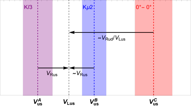
Figure 1: The purple, blue and red bands correspond respectively to the values of |Vu​s||V_{us}| from eq. (11), |Vu​s/Vu​d||V_{us}/V_{ud}| from eq. (13) and |Vu​d|=0.97376​(16)|V_{ud}|=0.97376(16) from eq. (15). The best fit point and 11, 22 and 3​σ3\sigma contours are shown (red cross and red circles) for these values. The black curve corresponds to the unitarity condition (8). The dashed black curve corresponds to eq. (9) with the deficit of unitarity δCKM=1.48⋅10−3\delta_{\text{CKM}}=1.48\cdot 10^{-3}. The green band correspond to the value |Vu​d|=0.97333​(47)|V_{ud}|=0.97333(47) obtained from neutron decay (17). The best fit point and 11 and 2​σ2\sigma contours (green cross and green circles) are obtained by fitting the latter determination with the other two determinations |Vu​s||V_{us}| from eq. (11), |Vu​s/Vu​d||V_{us}/V_{ud}| from eq. (13). The dashed gray curve corresponds to eq. (9) with the deficit of unitarity δCKM=2.6⋅10−3\delta_{\text{CKM}}=2.6\cdot 10^{-3}.

The tensions between determinations A, B and C are shown in figure 1, which presents the fit of the values (11), (13), (15), with Vu​sV_{us} and Vu​dV_{ud} considered as independent parameters, without imposing unitarity. The unitarity condition (8) is shown with the black continuous line. The best fit (minimum χ2\chi^{2}) corresponds to

|Vu​s|=0.22439​(36)|Vu​d|=0.97373​(16)\displaystyle|V_{us}|=0.22439(36)\qquad|V_{ud}|=0.97373(16) (18)

which is 3.6​σ3.6\sigma away from the unitarity curve. The χ2\chi^{2} value is rather large, χ2=7.4\chi^{2}=7.4, due to the tension between the two determinations A and B from kaon decays. For the deficit of CKM unitarity the best fit values (18) imply δCKM=1.48​(36)⋅10−3\delta_{\text{CKM}}=1.48(36)\cdot 10^{-3}.

The tensions can be manifested also in another way. We can take |Vu​s|A=0.22326​(55)|V_{us}|_{\text{A}}=0.22326(55) from the direct determination A while B and C can be also translated in |Vu​s||V_{us}| determinations by imposing the unitarity condition (8). Namely, the value of |Vu​s||V_{us}| obtained in this way from eq. (13) is:

|Vu​s|B=0.22535​(45)\displaystyle|V_{us}|_{\text{B}}=0.22535(45) (19)

which is compatible also with a theoretical result |Vu​s|=0.22567​(42)|V_{us}|=0.22567(42) from K​μ​2K\mu 2 decays obtained in ref. Martinelli.

From determination C (15) we get instead:

|Vu​s|C=0.22756​(70)\displaystyle|V_{us}|_{\text{C}}=0.22756(70) (20)

For completeness, in table 1 we show the values of |Vu​d||V_{ud}| and respective “unitarity” values of |Vu​s||V_{us}| corresponding to the choices of ΔR\Delta_{R} as reported in original refs. Marciano, Seng, Marciano2, indicated as C0, C1 and C2.

Figure 2 displays the values |Vu​s|A|V_{us}|_{\text{A}} (11), |Vu​s|B|V_{us}|_{\text{B}} (19) and |Vu​s|C|V_{us}|_{\text{C}} (20) with corresponding error bars (shaded areas). Between determinations obtained from kaon decays, A and B, there is 2.9​σ2.9\sigma tension, which maybe could disappear with more accurate lattice simulations.33 3 These determinations obtained from 3-flavor lattice computations FLAG2017 were in fact compatible because of larger error-bars, see figure 2. Therefore, we conservatively take a democratic average of |Vu​s|A|V_{us}|_{\text{A}} and |Vu​s|B|V_{us}|_{\text{B}} without reducing error bars (with the uncertainty taken as arithmetical average of two uncertainties):

A+B¯:|Vu​s|=0.22451​(50)\displaystyle\overline{\text{A+B}}\,:\qquad|V_{us}|=0.22451(50) (21)

We see that there is about 5​σ5\sigma tension between determination A and C and 3​σ3\sigma tension between B and C. The discrepancy of the average A+B¯\overline{\text{A+B}} from C results in 3.6​σ3.6\sigma. Let us notice that if we try to fit the incompatible determinations of Vu​sV_{us} AA (11), BB (19), CC (20), we would get the average value |Vu​s|=0.22511|V_{us}|=0.22511 but with a ugly large χ2\chi^{2} value, χ2=24\chi^{2}=24.

Determination    ΔR\Delta_{R}    |Vu​d||V_{ud}|    |Vu​s||V_{us}|
C0 Marciano    0.02361​(38)0.02361(38)    0.97420​(21)0.97420(21)    0.2257​(9)0.2257(9)
C1 Seng    0.02467​(22)0.02467(22)    0.97370​(14)0.97370(14)    0.22780​(60)0.22780(60)
C2 Marciano2    0.02426​(32)0.02426(32)    0.97389​(18)0.97389(18)    0.22699​(77)0.22699(77)
C (our choice)    0.02454​(27)0.02454(27)    0.97376​(16)0.97376(16)    0.22756​(70)0.22756(70)
Table 1: Values of ΔR\Delta_{R} reported in original references and corresponding values of |Vu​d||V_{ud}| obtained from eq. (14). Values of |Vu​s||V_{us}| are obtained assuming unitarity (8). C represents our ‘democratic’ average (see text).
Refer to caption
Figure 2: Shaded areas show the values of |Vu​s||V_{us}| obtained from determinations A (11), B (13) and C (15) by assuming CKM unitarity (8), while the black line corresponds to the democratic average of A and B (21) (see text). C0, C1, C2 are the values of |Vu​s||V_{us}| obtained from the values of ΔR\Delta_{R} reported by original references, as listed in table 1. For comparison we also show the values of |Vu​s||V_{us}| obtained using 33 flavours lattice QCD simulations as reported in FLAG 17 FLAG2017 and were adopted in Particle Data Group 2018. These determinations have practically no tension with the old determination C0 Marciano. Hence, this picture demonstrate that the CKM tensions in fact emerged due to improved precision of 44-flavours computations FLAG2019; Bazavov on one side, and due to the changes in inner radiative correction ΔR\Delta_{R} Seng; Marciano2 on the other side.
A: |Vu​s|=0.22326​(55)|V_{us}|\!=\!0.22326(55) B: |Vu​s|=0.23130​(49)​|Vu​d||V_{us}|\!=\!0.23130(49)|V_{ud}| Average∗
C1: |Vu​d|=0.97370​(14)|V_{ud}|\!=\!0.97370(14) 2.05​(37)⋅10−32.05(37)\cdot 10^{-3} 1.17​(35)⋅10−31.17(35)\cdot 10^{-3} 1.55​(36)⋅10−31.55(36)\cdot 10^{-3}
C2: |Vu​d|=0.97389​(18)|V_{ud}|\!=\!0.97389(18) 1.68​(43)⋅10−31.68(43)\cdot 10^{-3} 0.78​(41)⋅10−30.78(41)\cdot 10^{-3} 1.17​(42)⋅10−31.17(42)\cdot 10^{-3}
C:   |Vu​d|=0.97376​(16)|V_{ud}|\!=\!0.97376(16) 1.94​(40)⋅10−31.94(40)\cdot 10^{-3} 1.05​(38)⋅10−31.05(38)\cdot 10^{-3} 1.43​(39)⋅10−31.43(39)\cdot 10^{-3}
Table 2: Values of δCKM\delta_{\text{CKM}} obtained for different choices of the values of |Vu​s||V_{us}| and |Vu​d||V_{ud}|.
∗ We average the values of Vu​sV_{us} given in the columns A and B conservatively, taking its error bar as arithmetical average of their uncertainties.

In table 2 we show the landscape of possible values of the unitarity deficit δCKM\delta_{\text{CKM}}. We see that depending on the choice of the data this value spans from about 10−310^{-3} to about 2⋅10−32\cdot 10^{-3}.

In conclusion, it is clear that the CKM unitarity condition with three families (8) is inconsistent with the present determinations of |Vu​s||V_{us}| and |Vu​d||V_{ud}|. An immediate solution would be to introduce a fourth sequential family (t′,b′)(t^{\prime},b^{\prime}), analogous to the three SM families, with the LH components forming weak isodoublets and RH components being isosinglets. Then the 3×33\times 3 CKM matrix (1) should be extended to a unitary 4×44\times 4 matrix:

VCKM=(Vu​dVu​sVu​bVu​b′Vc​dVc​sVc​bVc​b′Vt​dVt​sVt​bVt​b′Vt′​dVt′​sVt′​bVt′​b′).\displaystyle V_{\text{CKM}}=\left(\begin{array}[]{cccc}V_{ud}&V_{us}&V_{ub}&V_{ub^{\prime}}\\ V_{cd}&V_{cs}&V_{cb}&V_{cb^{\prime}}\\ V_{td}&V_{ts}&V_{tb}&V_{tb^{\prime}}\\ V_{t^{\prime}d}&V_{t^{\prime}s}&V_{t^{\prime}b}&V_{t^{\prime}b^{\prime}}\end{array}\right).

and correspondingly the first row unitarity condition would be modified to:

|Vu​d|2+|Vu​s|2+|Vu​b|2+|Vu​b′|2=1\displaystyle|V_{ud}|^{2}+|V_{us}|^{2}+|V_{ub}|^{2}+|V_{ub^{\prime}}|^{2}=1 (26)

Comparing this equation with eq. (9) we see that the parameter δCKM\delta_{\text{CKM}} assumes the meaning of the mixing with the fourth family, δCKM=|Vu​b′|2\delta_{\text{CKM}}=|V_{ub^{\prime}}|^{2}. Therefore for typical values of δCKM\delta_{\text{CKM}} given in table 2 we get |Vu​b′|≈0.04|V_{ub^{\prime}}|\approx 0.04, which is comparable with |Vc​b||V_{cb}| and an order of magnitude larger than |Vu​b|≈0.004|V_{ub}|\approx 0.004. It looks not very natural that the mixing of the first family with fourth family is much stronger than its mixing with third family, but some models admit this possibility Bregar. Unfortunately, the existence of a fourth sequential family is excluded by the limits from electroweak precision data combined with the LHC data.

However, vector-like quarks can be introduced without any contradiction with SM precision tests. The LHC limits merely tell that their masses should be above 11 TeV or so.

In the rest of this paper we discuss how the anomalies in the first row of CKM matrix can be solved by introducing extra vector-like fermions. In particular we will consider the role of weak isosinglets of down-type or up-type and weak isodoublets.

In fact, two approaches to the problem can be considered. The incompatibility inside kaon physics may be attributed to some uncertainties which can disappear maybe soon with more precise determinations, focusing instead on the average of determinations from kaons. Then the problem consist in solving the lack of unitarity in the first row of VCKMV_{\text{CKM}}. The insertion of an extra vectorlike weak isosinglet, down-type or up-type, is on this line.

Otherwise the discrepancy inside kaon physics can be considered seriously by looking for a solution addressing the whole situation. However, the Vu​sV_{us} anomaly (discrepancy between Vu​sV_{us} determinations from the kaon semileptonic and leptonic decays) can be considered seriously, 44 4 In fact, a recent high precision determination of K​ℓ​3K\ell 3 radiative corretions Seng:2021boy indicates that the SM electroweak effects are not large enough to account for Vu​sV_{us} anomaly. and one has to look for a solution addressing the whole situation. As it will be shown, a weak isodoublet can in principle explain all the anomalies.

In these scenarios with extra vector-like families, the unitarity deficit δCKM\delta_{\text{CKM}} will be related to the mixing of the extra quarks with the SM families.

3 The SM with extra vector-like fermions

The Standard Model S​U​(3)×S​U​(2)×U⁡(1)SU(3)\times SU(2)\times U(1) contains, by definition, three chiral families of fermions, the LH quarks qL​i=(uL,dL)iq_{Li}=(u_{L},d_{L})_{i} and leptons ℓL​i=(νL,eL)i\ell_{Li}=(\nu_{L},e_{L})_{i} transforming as S​U​(2)SU(2) isodoublets and the RH components uR​iu_{Ri}, dR​id_{Ri}, eR​ie_{Ri} being isosinglets, with i=1,2,3i=1,2,3 being the family index. This set of fermions is free of gauge anomalies. Attractive property of the SM is that these fermions can acquire masses only via the Yukawa couplings with Higgs doublet φ\varphi:

ℒYukSM=Yui​j​φ~​qL​i¯​uR​j+Ydi​j​φ​qL​i¯​dR​j+Yei​j​φ​ℓL​i¯​eR​j+h.c.\displaystyle{\cal L}_{\rm Yuk}^{\rm SM}=Y_{u}^{ij}\tilde{\varphi}\,\overline{q_{Li}}u_{Rj}+Y_{d}^{ij}\varphi\,\overline{q_{Li}}d_{Rj}+Y_{e}^{ij}\varphi\,\overline{\ell_{Li}}e_{Rj}\penalty\ +\penalty\ {\rm h.c.} (27)

where Yu,d,ei​jY_{u,d,e}^{ij} are the Yukawa constant matrices, and φ~=i​τ2​φ∗\tilde{\varphi}=i\tau_{2}\varphi^{\ast}. The known species of quarks and leptons are eigenstates of mass matrices Mu,d,e=Yu,d,e​vwM_{u,d,e}=Y_{u,d,e}v_{w} where ⟨φ0⟩=vw\langle\varphi^{0}\rangle=v_{w} is the Higgs VEV. In other words, in the SM the quark and lepton masses are induced only after the electroweak symmetry breaking, and their values are proportional to the electroweak scale vwv_{w}.

The quark mass matrices can be diagonalized by bi-unitary transformations

VL​u†​Mu​VR​u=M~u=diag⁡(mu,mc,mt),VL​d†​Md​VR​d=M~d=diag⁡(md,ms,mb)\displaystyle V_{Lu}^{\dagger}M_{u}V_{Ru}=\widetilde{M}_{u}={\rm diag}(m_{u},m_{c},m_{t}),\quad V_{Ld}^{\dagger}M_{d}V_{Rd}=\widetilde{M}_{d}={\rm diag}(m_{d},m_{s},m_{b}) (28)

and the weak eigenstates in terms of mass eigenstates are:

(uL​1uL​2uL​3)=VL​u​(uLcLtL);\displaystyle\left(\begin{array}[]{c}u_{L1}\\ u_{L2}\\ u_{L3}\end{array}\right)=V_{Lu}\left(\begin{array}[]{c}u_{L}\\ c_{L}\\ t_{L}\end{array}\right); (dL​1dL​2dL​3)=VL​d​(dLsLbL)\displaystyle\left(\begin{array}[]{c}d_{L1}\\ d_{L2}\\ d_{L3}\end{array}\right)=V_{Ld}\left(\begin{array}[]{c}d_{L}\\ s_{L}\\ b_{L}\end{array}\right)

The CKM mixing matrix in WW boson charged current couplings (1) emerges as a combination of the ‘left’ unitary transformations, VCKM=VL​u†​VL​dV_{\rm CKM}=V_{Lu}^{\dagger}V_{Ld}, and thus it should be unitary. As for the ‘right’ matrices VR​uV_{Ru} and VR​dV_{Rd}, in the SM frames they have no physical significance. Without loss of generality, one can choose a fermion basis in which one of the Yukawa matrices YuY_{u} or YdY_{d} is diagonal in which cases we would have respectively VCKM=VL​dV_{\rm CKM}=V_{Ld} or VCKM=VL​u†V_{\rm CKM}=V_{Lu}^{\dagger}.

The SM exhibits a remarkable feature of natural suppression of flavor-changing neutral currents (FCNC) Glashow; Paschos: no flavor mixing emerges in neutral currents coupled to ZZ boson and Higgs boson. In particular, this means that ZZ boson tree level couplings with the fermion mass eigenstates remain diagonal after rotations (3). On the other hand, the Yukawa matrices Yu,d,eY_{u,d,e} and mass matrices Mu,d,eM_{u,d,e} are proportional and thus by transformations (28) they are diagonalized simultaneously, so that the Yukawa couplings of the Higgs boson HH with the fermion mass eigenstates are diagonal. Hence, all FCNC phenomena are suppressed at tree level and emerge exclusively from radiative corrections. At present, the majority of experimental data on flavor changing and CP violating processes are in good agreement with the SM predictions.

Clearly, in the SM framework the unitarity of the CKM matrix as well as the natural flavor conservation in neutral currents are direct consequences following from the fact that the three families are in identical representations of S​U​(3)×S​U​(2)×U⁡(1)SU(3)\times SU(2)\times U(1).

However, in addition to three chiral families of quarks and leptons, there can exist extra vector-like species, with the LH and RH in the same representations of the SM. In particular, one can consider the extra fermion species in the same representations of S​U​(3)×S​U​(2)×U⁡(1)SU(3)\times SU(2)\times U(1) as standard quarks and leptons, namely in the form of weak isosinglets of down quark type DL,RD_{L,R}, up quark type UL,RU_{L,R} and charged lepton type EL,RE_{L,R}, and weak isodoublets QL,R=(𝒰,𝒟)L,RQ_{L,R}=({\cal U},{\cal D})_{L,R} and LL,R=(𝒩,ℰ)L,RL_{L,R}=({\cal N},{\cal E})_{L,R} of quark and lepton types.55 5 Such vector-like species are predicted in some extensions of the Standard Model. For example, DD and LL type species emerge (per each family) in the context of minimal E6E_{6} Gursey; Achiman or S​U​(6)SU(6) Dvali grand unifications. In addition, the specifics of the latter model in which Higgs emerges as pseudo-Goldstone particle, requires at least one copy of QQ, UU and EE type species for inducing the fermion masses and in particular the top quark mass Barbieri; su6. (Extra vector-like fermions can be introduced also in other representations as e.g. S​U​(2)SU(2) isotriplets which can contain quark or lepton type fragments but also some fragments with exotic electric charges but here we do not address these cases.) The mass terms of these species are not protected by the SM gauge symmetries and hence their masses can be (or must be) considerably larger than the electroweak scale.

In the following we shall concentrate on the quark sector. Namely, we consider a theory which, besides the three chiral families of standard quarks uR​iu_{Ri}, dR​id_{Ri} and qL​i=(uL,dL)iq_{Li}=(u_{L},d_{L})_{i} (i=1,2,3i=1,2,3), includes some extra vector-like quark species UL,RU_{L,R}, DL,RD_{L,R} and QL,R=(𝒰,𝒟)L,RQ_{L,R}=({\cal U},{\cal D})_{L,R} which in principle can be introduced in different amounts. Therefore, along with the standard Yukawa terms for the three chiral families:66 6 Hereafter indices i=1,2,3i=1,2,3 of normal families as well as indices of extra species are suppressed.

ℒYuk=Yu​φ~​qL¯​uR+Yd​φ​qL¯​dR+h.c.\displaystyle{\cal L}_{\rm Yuk}=Y_{u}\tilde{\varphi}\,\overline{q_{L}}u_{R}+Y_{d}\varphi\,\overline{q_{L}}d_{R}\penalty\ +\penalty\ {\rm h.c.} (41)

the most general Lagrangian of this system must include the mixed Yukawa terms between the standard and extra species:

ℒYukmix=hU​φ~​qL¯​UR+hD​φ​qL¯​DR+h𝒰​φ~​QL¯​uR+h𝒟​φ​QL¯​dR+h.c.\displaystyle{\cal L}_{\rm Yuk}^{\rm mix}=h_{U}\tilde{\varphi}\,\overline{q_{L}}U_{R}+h_{D}\varphi\,\overline{q_{L}}D_{R}+h_{\cal U}\tilde{\varphi}\,\overline{Q_{L}}u_{R}+h_{\cal D}\varphi\,\overline{Q_{L}}d_{R}\penalty\ +\penalty\ {\rm h.c.} (42)

and the mass terms

ℒmass=MU​UL¯​UR+MD​DL¯​DR+MQ​QL¯​QR+μu​UL¯​uR+μd​DL¯​dR+μq​qL¯​QR+h.c.\displaystyle{\cal L}_{\rm mass}=M_{U}\overline{{U}_{L}}{U}_{R}+M_{D}\overline{{D}_{L}}{D}_{R}+M_{Q}\overline{Q_{L}}Q_{R}+\mu_{u}\overline{{U}_{L}}u_{R}+\mu_{d}\overline{{D}_{L}}d_{R}+\mu_{q}\overline{q_{L}}Q_{R}\penalty\ +\penalty\ {\rm h.c.} (43)

where hU,Dh_{U,D} and hu,dh_{u,d} in the Yukawa terms (42) and MU,D,QM_{U,D,Q} and μu,d,q\mu_{u,d,q} in mass terms (43) are the matrices of proper dimensions depending on the amounts of extra species. One could introduce also the Yukawa couplings between extra species:

ℒYukextra=λU​φ~​QL¯​UR+λ𝒰​φ~​QR¯​UL+λD​φ​QL¯​DR+λ𝒟​φ​QR¯​DL+h.c.\displaystyle{\cal L}_{\rm Yuk}^{\rm extra}=\lambda_{U}\tilde{\varphi}\,\overline{Q_{L}}U_{R}+\lambda_{\cal U}\tilde{\varphi}\,\overline{Q_{R}}U_{L}+\lambda_{D}\varphi\,\overline{Q_{L}}D_{R}+\lambda_{\cal D}\varphi\,\overline{Q_{R}}D_{L}\penalty\ +\penalty\ {\rm h.c.} (44)

However, they play no relevant role in further discussions and for simplicity we neglect them.

The vector-like quarks are key players in models with horizontal inter-family symmetries PLB83; Dimopoulos; PLB85; Bagger; Khlopov1; Khlopov2; King; so10, in some models of the axion Kim; Shifman; Khlopov; Zphys; Sakharov as well as in axionless (Nelson-Barr type) models for solving the strong CP problem via spontaneous CP or P violation Nelson; Barr; Babu; MPL; Senjanovic. In these models the values MU,D,QM_{U,D,Q} and μu,d,q\mu_{u,d,q} in mass terms (43) are related to the breaking scales of respective symmetries, and in some models e.g. Babu; Senjanovic; Berezhiani:1990 they can be as low as few TeV.

Interestingly, some of these symmetries (e.g. flavor symmetry or Peccei-Quinn symmetry) may forbid the direct Yukawa terms (41) but allow the mixed ones (42) while mass terms μ\mu and MM in (42) can be originated from some physical scales.77 7 E.g. in the ‘seesaw’ model of ref. PLB83 the values of μu,d\mu_{u,d} and MU,DM_{U,D} are respectively determined by the breaking scales of left-right symmetry and family symmetry, i.e. by the VEV of the ‘right’ Higgs doublet and VEVs of flavon scalars which break the horizontal symmetry. Nevertheless, despite that the original constants Yu,dY_{u,d} in (41) are vanishing, the SM Yukawa terms (27) for normal fermions will be induced after integrating out the heavy states. In particular, provided that mixing mass terms μu,d,q\mu_{u,d,q} are smaller than MU,D,QM_{U,D,Q}, we obtain

Yu≃hU​MU−1​μu+μq​MQ−1​h𝒰,Yd≃hD​MD−1​μd+μq​MQ−1​h𝒟\displaystyle Y_{u}\simeq h_{U}M_{U}^{-1}\mu_{u}+\mu_{q}M_{Q}^{-1}h_{\cal U},\quad Y_{d}\simeq h_{D}M_{D}^{-1}\mu_{d}+\mu_{q}M_{Q}^{-1}h_{\cal D} (45)

In other words, the non-zero quark masses are induced via the mixings with the extra vector-like species. Such a scenario known as ‘universal’ seesaw mechanism PLB83; Rajpoot; Davidson; Rattazzi is commonly used in predictive model building for fermion masses and mixings as e.g. PLB83; Rattazzi; Rattazzi2; tanbeta; Anderson:1993fe; Berezhiani:1996bv; Koide1; Koide2; Nesti. In the context of supersymmetric models with flavor symmetry this mechanism can give a natural realization of the minimal flavor violation scenario via the alignment of soft supersymmetry breaking terms with the Yukawa terms MFV; MFV1; MFV2.

In the following we are not interested in the model details and in possible dynamical effects of the underlying symmetries broken at higher scales, but only in the effects of the mixing between the three normal (chiral) and extra (vector-like) quarks. Therefore, we can conveniently redefine the fermion basis. Namely, the species uRu_{R} and URU_{R}, dRd_{R} and DRD_{R}, and qLq_{L} and QLQ_{L}, are in the identical representations of S​U​(3)×S​U​(2)×U⁡(1)SU(3)\times SU(2)\times U(1). Thus, by redefining these species, one can eliminate mixed mass terms μu\mu_{u}, μd\mu_{d} and μq\mu_{q} in (43) by ‘absorbing’ them respectively in the mass terms MUM_{U}, MDM_{D} and MQM_{Q} (this means that e.g. from 3+n3+n RH species with quantum numbers of dRd_{R} we can always select nn their combinations which ‘marry’ nn species of LH fermions 𝒟L{\cal D}_{L} via mass terms while the remaining 33 combinations have no mass terms). In addition, without losing generality, the ‘heavy’ mass matrices MUM_{U}, MDM_{D} and MQM_{Q} can be taken to be diagonal and real.

In this basis the total mass matrices of up type (u,U,𝒰)L,R(u,U,{\cal U})_{L,R} and down type (d,D,𝒟)L,R(d,D,{\cal D})_{L,R} quarks, after substituting the Higgs VEV ⟨ϕ⟩=vw\langle\phi\rangle=v_{w}, read:

ℳup=(Yu​vwhU​vw00MU0h𝒰​vw0MQ),ℳdown=(Yd​vwhD​vw00MD0h𝒟​vw0MQ)\displaystyle{\cal M}_{\rm up}=\left(\begin{array}[]{ccc}Y_{u}v_{w}&h_{U}v_{w}&0\\ 0&M_{U}&0\\ h_{\cal U}v_{w}&0&M_{Q}\end{array}\right),\quad\quad{\cal M}_{\rm down}=\left(\begin{array}[]{ccc}Y_{d}v_{w}&h_{D}v_{w}&0\\ 0&M_{D}&0\\ h_{\cal D}v_{w}&0&M_{Q}\end{array}\right)

where the blocks Yu,dY_{u,d} are matrices of dimensions 3×33\times 3. Assuming that the numbers of extra species UU, DD and QQ are respectively pp, nn and mm, then blocks MUM_{U}, MDM_{D} and MQM_{Q} should be correspondingly of dimensions p×pp\times p, n×nn\times n and m×mm\times m. Thus, ℳup{\cal M}_{\rm up} and ℳdown{\cal M}_{\rm down} respectively are (3+p+m)×(3+p+m)(3+p+m)\times(3+p+m) and (3+n+m)×(3+n+m)(3+n+m)\times(3+n+m) matrices.

The mass matrices (3) can be brought to the diagonal forms via bi-unitary transformations (𝒱upL)†​ℳup​𝒱upR=ℳ~up({\cal V}^{L}_{\rm up})^{\dagger}{\cal M}_{\rm up}{\cal V}^{R}_{\rm up}=\widetilde{\cal M}_{\rm up} and (𝒱downL)†​ℳdown​𝒱downR=ℳ~down({\cal V}^{L}_{\rm down})^{\dagger}{\cal M}_{\rm down}{\cal V}^{R}_{\rm down}=\widetilde{\cal M}_{\rm down}. In this way, the initial states of e.g. down-type quarks are related to their physical states (mass eigenstates) as

(dD𝒟)L,R=𝒱downL,R​(d′D′𝒟′)L,R=(Vd​d′L,RVd​D′L,RVd​𝒟′L,RVD​d′L,RVD​D′L,RVD​𝒟′L,RV𝒟​d′L,RV𝒟​D′L,RV𝒟𝒟′L,R)​(d′D′𝒟′)L,R\displaystyle\left(\begin{array}[]{c}d\\ D\\ {\cal D}\end{array}\right)_{\!\!L,R}={\cal V}_{\rm down}^{L,R}\left(\begin{array}[]{c}d^{\prime}\\ D^{\prime}\\ {\cal D}^{\prime}\end{array}\right)_{\!\!L,R}=\left(\begin{array}[]{ccc}V_{dd^{\prime}}^{L,R}&V_{dD^{\prime}}^{L,R}&V_{d{\cal D}^{\prime}}^{L,R}\\ V_{Dd^{\prime}}^{L,R}&V_{DD^{\prime}}^{L,R}&V_{D{\cal D}^{\prime}}^{L,R}\\ V_{{\cal D}d^{\prime}}^{L,R}&V_{{\cal D}D^{\prime}}^{L,R}&V_{{\cal D}{\cal D}^{\prime}}^{L,R}\end{array}\right)\left(\begin{array}[]{c}d^{\prime}\\ D^{\prime}\\ {\cal D}^{\prime}\end{array}\right)_{\!\!L,R}

Here d=(d1,d2,d3)Td=(d_{1},d_{2},d_{3})^{T} are initial states and d′=(d,s,b)Td^{\prime}=(d,s,b)^{T} are the mass eigenstates, and similarly for heavy species DD and 𝒟{\cal D}. Analogously, unitary matrices 𝒱upL,R{\cal V}^{L,R}_{\rm up} connect the initial up-quark type states u,U,𝒰u,U,{\cal U} with their mass eigenstates u′,U′,𝒰′u^{\prime},U^{\prime},{\cal U}^{\prime}, where u=(u1,u2,u3)Tu=(u_{1},u_{2},u_{3})^{T} and u′=(u,c,t)Tu^{\prime}=(u,c,t)^{T}.

Since we have ℳ~down2=(𝒱downL)†​ℳdown​ℳdown†​𝒱downL=(𝒱downR)†​ℳdown†​ℳdown​𝒱downR\widetilde{\cal M}_{\rm down}^{2}=({\cal V}^{L}_{\rm down})^{\dagger}\,{\cal M}_{\rm down}{\cal M}_{\rm down}^{\dagger}\,{\cal V}^{L}_{\rm down}=({\cal V}^{R}_{\rm down})^{\dagger}\,{\cal M}_{\rm down}^{\dagger}{\cal M}_{\rm down}\,{\cal V}^{R}_{\rm down}, unitary matrices 𝒱downL{\cal V}^{L}_{\rm down} and 𝒱downR{\cal V}^{R}_{\rm down} can be determined by considering the hermitean squares of ℳdown{\cal M}_{\rm down}:

ℳdown​ℳdown†=(vw2​Yd​Yd†+vw2​hD​hD†vw​hD​MDvw2​Yd​h𝒟†vw​MD​hD†MD20vw2​h𝒟​Yd†0MQ2+vw2​h𝒟​h𝒟†),\displaystyle{\cal M}_{\rm down}{\cal M}_{\rm down}^{\dagger}=\left(\begin{array}[]{ccc}v_{w}^{2}Y_{d}Y_{d}^{\dagger}+v_{w}^{2}h_{D}h_{D}^{\dagger}&v_{w}h_{D}M_{D}&v_{w}^{2}Y_{d}h_{\cal D}^{\dagger}\\ v_{w}M_{D}h_{D}^{\dagger}&M_{D}^{2}&0\\ v_{w}^{2}h_{\cal D}Y_{d}^{\dagger}&0&M_{Q}^{2}+v_{w}^{2}h_{\cal D}h_{\cal D}^{\dagger}\end{array}\right),
ℳdown†​ℳdown=(vw2​Yd†​Yd+vw2​h𝒟†​h𝒟vw2​Yd†​hDvw​h𝒟†​MQvw2​hD†​YdMD2+vw2​hD†​hD0vw​MQ​h𝒟0MQ2).\displaystyle{\cal M}_{\rm down}^{\dagger}{\cal M}_{\rm down}=\left(\begin{array}[]{ccc}v_{w}^{2}Y_{d}^{\dagger}Y_{d}+v_{w}^{2}h_{\cal D}^{\dagger}h_{\cal D}&v^{2}_{w}Y_{d}^{\dagger}h_{D}&v_{w}h_{\cal D}^{\dagger}M_{Q}\\ v_{w}^{2}h_{D}^{\dagger}Y_{d}&M_{D}^{2}+v_{w}^{2}h_{D}^{\dagger}h_{D}&0\\ v_{w}M_{Q}h_{\cal D}&0&M_{Q}^{2}\end{array}\right)\,.

The off-diagonal entries of these matrices are fixed by the value vwv_{w}, so that the elements of the off-diagonal blocks Vd​D′V_{dD^{\prime}}, Vd​𝒟′V_{d{\cal D}^{\prime}} etc. in (3) are determined by the ratio of the electroweak scale to the masses of extra quark species. In the limit when the latter are very heavy they decouple and their mixings with light quarks become negligibly small. Thus, in this limit 3×33\times 3 block Vd​d′V_{dd^{\prime}} becomes unitary. The same is true for analogous Vu​u′V_{uu^{\prime}} block in up quark mixing. However, if the extra quarks are not that heavy and off-diagonal blocks are not negligible, then Vd​d′V_{dd^{\prime}} and Vu​u′V_{uu^{\prime}} blocks are no more unitary.

The present experimental limits on the extra quark masses are MU,D,Q>(1÷1.5)M_{U,D,Q}>(1\div 1.5) TeV, depending on their type and decay modes PDG18. Therefore, the ratios ϵu=vw/MU\epsilon_{u}=v_{w}/M_{U}, ϵd=vw/MD\epsilon_{d}=v_{w}/M_{D} and ϵq=vw/MQ\epsilon_{q}=v_{w}/M_{Q} can be considered as small parameters, ϵu,d,q≤0.1\epsilon_{u,d,q}\leq 0.1 or so. By inspecting the matrices (3), one can estimate the elements of the off-diagonal blocks in 𝒱L,Rdown{\cal V}_{L,R}^{\rm down} and 𝒱L,Rup{\cal V}_{L,R}^{\rm up} as

|Vd​D′L|∼ϵd,|Vu​U′L|∼ϵu,\displaystyle|V^{L}_{dD^{\prime}}|\sim\epsilon_{d},\quad|V^{L}_{uU^{\prime}}|\sim\epsilon_{u}, |Vd​𝒟′L|,|Vu​𝒰′L|∼ϵq2\displaystyle\qquad|V^{L}_{d{\cal D}^{\prime}}|,|V^{L}_{u{\cal U}^{\prime}}|\sim\epsilon_{q}^{2}\qquad
|Vd​𝒟′R|,|Vu​𝒰′R|∼ϵq,\displaystyle\qquad|V^{R}_{d{\cal D}^{\prime}}|,|V^{R}_{u{\cal U}^{\prime}}|\sim\epsilon_{q}, |Vd​D′R|∼ϵd2,|Vu​U′R|∼ϵu2\displaystyle|V^{R}_{dD^{\prime}}|\sim\epsilon_{d}^{2},\quad|V^{R}_{uU^{\prime}}|\sim\epsilon_{u}^{2}\qquad (70)

modulo the Yukawa constants which are assumed to be ≤1\leq 1 for perturbativity. Therefore, the deviation from unitarity of the “left" matrices Vd​d′LV_{dd^{\prime}}^{L} and Vu​u′LV_{uu^{\prime}}^{L} blocks are ∼ϵu,d2≤10−2\sim\epsilon^{2}_{u,d}\leq 10^{-2}. E.g. the first row unitarity of the matrix 𝒱downL{\cal V}^{L}_{\rm down} implies |V1​d|2+|V1​s|2+|V1​b|2=1−|V1​D′|2−|V1​𝒟′|2=1−δd|V_{1d}|^{2}+|V_{1s}|^{2}+|V_{1b}|^{2}=1-|V_{1D^{\prime}}|^{2}-|V_{1{\cal D}^{\prime}}|^{2}=1-\delta_{d}. Taking into account the above estimations, we see that the deviation can be as large as δd∼ϵd2∼10−2\delta_{d}\sim\epsilon_{d}^{2}\sim 10^{-2}. Let us recall that the CKM unitarity deficit δCKM\delta_{\rm CKM} estimated in previous section is about (1÷2)×10−3(1\div 2)\times 10^{-3}, see table 2. Thus, for accounting for the above values of δCKM\delta_{\rm CKM}, one would need ϵd=0.03−0.05\epsilon_{d}=0.03-0.05. As for ϵ4∼10−4\epsilon^{4}\sim 10^{-4} contributions, they are irrelevant and so order ϵ2\epsilon^{2} mixings as V1​𝒟′V_{1{\cal D}^{\prime}} etc. can be safely neglected.

Let us assume, for simplicity, that each of UU, DD and QQ type species is present in one copy, i.e. p=m=n=1p=m=n=1 (our discussion can be extended in a straightforward way for arbitrary number of extra species). In this case the off-diagonal blocks proportional to vwv_{w} in 5×55\times 5 matrices (3) become columns as e.g. hD=(h1​D,h2​D,h3​D)Th_{D}=(h_{1D},h_{2D},h_{3D})^{T} or rows as e.g. h𝒟=(h𝒟​1,h𝒟​2,h𝒟​3)h_{\cal D}=(h_{{\cal D}1},h_{{\cal D}2},h_{{\cal D}3}). The Yukawa couplings Yu,dY_{u,d} can be presented in the form Yu=VL​u​Y~u​VR​u†Y_{u}=V_{Lu}\widetilde{Y}_{u}V_{Ru}^{\dagger} and Yd=VL​d​Y~d​VR​d†Y_{d}=V_{Ld}\widetilde{Y}_{d}V_{Rd}^{\dagger} where Y~u,d\widetilde{Y}_{u,d} are diagonal 3×33\times 3 matrices, Y~u=diag⁡(yu,yc,yt)\widetilde{Y}_{u}={\rm diag}(y_{u},y_{c},y_{t}) and Y~d=diag⁡(yd,ys,yb)\widetilde{Y}_{d}={\rm diag}(y_{d},y_{s},y_{b}). Let us denote also hU=VL​u​h~Uh_{U}=V_{Lu}\widetilde{h}_{U}, hD=VL​d​h~Dh_{D}=V_{Ld}\widetilde{h}_{D}, h𝒰=h~𝒰​VR​u†h_{\cal U}=\widetilde{h}_{\cal U}V_{Ru}^{\dagger} and h𝒟=h~𝒟​VR​d†h_{\cal D}=\widetilde{h}_{\cal D}V_{Rd}^{\dagger}.

Then for 5×55\times 5 unitary matrix of ‘left’ rotations we obtain, with the precision up to ϵ2\epsilon^{2} terms:

𝒱downL=(VL​d00010001)​(1−SD​SD†SD0−SD†1−SD†​SD0001)​(1−S𝒟​S𝒟†0S𝒟010−S𝒟†01−S𝒟†​S𝒟)\displaystyle{\cal V}_{\rm down}^{L}=\left(\begin{array}[]{ccc}V_{Ld}&0&0\\ 0&1&0\\ 0&0&1\end{array}\right)\!\left(\begin{array}[]{ccc}\!\!\!\sqrt{1-S_{D}S_{D}^{\dagger}}&S_{D}&0\\ -S_{D}^{\dagger}&\!\!\sqrt{1-S_{D}^{\dagger}S_{D}}&0\\ 0&0&1\end{array}\right)\!\left(\begin{array}[]{ccc}\!\!\!\sqrt{1-S_{\cal D}S_{\cal D}^{\dagger}}&0&S_{\cal D}\\ 0&1&0\\ -S_{\cal D}^{\dagger}&0&\sqrt{1-S_{\cal D}^{\dagger}S_{\cal D}}\end{array}\right)
=(VL​d​[1−12​SD​SD†−12​S𝒟​S𝒟†+…]VL​d​SDVL​d​S𝒟−SD†1−12​SD†​SD+…O⁡(ϵd​ϵq2)−S𝒟†01−12​S𝒟†​S𝒟+…)\displaystyle\quad\quad\quad=\left(\begin{array}[]{ccc}V_{Ld}\big[1-\frac{1}{2}S_{D}S_{D}^{\dagger}-\frac{1}{2}S_{\cal D}S_{\cal D}^{\dagger}+\dots\big]&V_{Ld}S_{D}&V_{Ld}S_{\cal D}\\ -S_{D}^{\dagger}&1-\frac{1}{2}S_{D}^{\dagger}S_{D}+\dots&O(\epsilon_{d}\epsilon_{q}^{2})\\ -S_{\cal D}^{\dagger}&0&1-\frac{1}{2}S_{\cal D}^{\dagger}S_{\cal D}+\dots\end{array}\right)

where the column SD=ϵd​h~DS_{D}=\epsilon_{d}\widetilde{h}_{D} describes the light quark (d,s,bd,s,b) mixings with the extra isosinglet species DD. As for their mixings with 𝒟⊂Q{\cal D}\subset Q from extra isodoublet, S𝒟=ϵq2​Y~d​h~𝒟†S_{\cal D}=\epsilon_{q}^{2}\widetilde{Y}_{d}\widetilde{h}_{\cal D}^{\dagger}, it can be neglected since, apart of ϵ2\epsilon^{2} suppression, these are proportional to the small Yukawa constants yd,ys,yby_{d},y_{s},y_{b} in Y~d\widetilde{Y}_{d}. Clearly, the unitarity conditions for rows and columns of this matrix is fulfilled with the precision up to ∼ϵd4\sim\epsilon_{d}^{4} terms. The matrix 𝒱upL{\cal V}_{\rm up}^{L} can be presented in an analogous form.

Let us discuss now charged current interactions. Considering that qLq_{L} and QLQ_{L} are S​U​(2)SU(2) doublets while ULU_{L} and DLD_{L} are singlets, the LH charged current interacting with WW boson in terms of initial states and mass eigenstates reads:

g2​Wμ+​(uL​UL​𝒰L)¯​γμ​JL​(dLDL𝒟L)=g2​2​Wμ+​(u′U′𝒰′)¯​γμ​(1−γ5)​𝒱Lmix​(d′D′𝒟′)\displaystyle\frac{g}{\sqrt{2}}\,W^{+}_{\mu}\,\overline{(u_{L}\penalty\ U_{L}\penalty\ {\cal U}_{L})}\,\gamma^{\mu}\,J_{L}\left(\begin{array}[]{c}d_{L}\\ D_{L}\\ {\cal D}_{L}\end{array}\right)=\frac{g}{2\sqrt{2}}\,W^{+}_{\mu}\,\overline{(u^{\prime}\penalty\ \penalty\ U^{\prime}\penalty\ \penalty\ {\cal U}^{\prime})}\,\gamma^{\mu}(1-\gamma^{5})\,{\cal V}_{L}^{\rm mix}\left(\begin{array}[]{c}d^{\prime}\\ D^{\prime}\\ {\cal D}^{\prime}\end{array}\right)

where JL=diag⁡(1,1,1,0,1)J_{L}={\rm diag}(1,1,1,0,1) and 𝒱Lmix=(𝒱Lup)†​JL​𝒱Ldown{\cal V}_{L}^{\rm mix}=({\cal V}_{L}^{\rm up})^{\dagger}J_{L}{\cal V}_{L}^{\rm down}, or explicitly

𝒱Lmix=((1−12​ΔU)​V~​(1−12​ΔD)(1−12​ΔU)​V~​SDO⁡(ϵ2)SU†​V~​(1−12​ΔD)SU†​V~​SDO⁡(ϵ3)O⁡(ϵ2)O⁡(ϵ3)1),V~=VL​u†​VL​d\displaystyle{\cal V}^{\rm mix}_{L}=\left(\begin{array}[]{ccc}\!\!(1-\frac{1}{2}\Delta_{U})\widetilde{V}(1-\frac{1}{2}\Delta_{D})&(1-\frac{1}{2}\Delta_{U})\widetilde{V}S_{D}&O(\epsilon^{2})\\ S_{U}^{\dagger}\widetilde{V}(1-\frac{1}{2}\Delta_{D})&S_{U}^{\dagger}\widetilde{V}S_{D}&O(\epsilon^{3})\\ O(\epsilon^{2})&O(\epsilon^{3})&1\end{array}\right)\!,\quad\widetilde{V}=V_{Lu}^{\dagger}V_{Ld}

where ΔU=SU​SU†=ϵu2​h~U​h~U†\Delta_{U}=S_{U}S_{U}^{\dagger}=\epsilon_{u}^{2}\widetilde{h}_{U}\widetilde{h}_{U}^{\dagger} and ΔD=SD​SD†=ϵd2​h~D​h~D†\Delta_{D}=S_{D}S_{D}^{\dagger}=\epsilon_{d}^{2}\widetilde{h}_{D}\widetilde{h}_{D}^{\dagger} as far as O⁡(ϵq4)O(\epsilon_{q}^{4}) contributions S𝒰​S𝒰†S_{\cal U}S_{\cal U}^{\dagger} and S𝒟​S𝒟†S_{\cal D}S_{\cal D}^{\dagger} can be neglected.

We are interested in its 3×33\times 3 block which describes the transitions between the quark mass eigenstates u′=(u,c,t)u^{\prime}=(u,c,t) and d′=(d,s,b)d^{\prime}=(d,s,b) in charged current:

VCKM=(1−12​ΔU)​V~​(1−12​ΔD)=(Vu​dVu​sVu​bVc​dVc​sVc​bVt​dVt​sVt​b)\displaystyle V_{\text{CKM}}=\big(1-\frac{1}{2}\Delta_{U}\big)\,\widetilde{V}\,\big(1-\frac{1}{2}\Delta_{D}\big)=\left(\begin{array}[]{ccc}V_{ud}&V_{us}&V_{ub}\\ V_{cd}&V_{cs}&V_{cb}\\ V_{td}&V_{ts}&V_{tb}\end{array}\right)

While V~=VL​u†​VL​d\widetilde{V}=V_{Lu}^{\dagger}V_{Ld} is unitary 3×33\times 3 matrix, the ‘corrected’ matrix VCKMV_{\rm CKM} is not. In particular, deviation from the unitarity for its rows or columns read, up to order ϵ2\epsilon^{2} terms, respectively as88 8 Obviously, the ‘large’ mixing matrix 𝒱Lmix{\cal V}^{\rm mix}_{L} is not unitary in itself because of the non-unitary factor JLJ_{L} ‘sandwiched’ between the unitary matrices 𝒱Lup{\cal V}^{\rm up}_{L} and 𝒱Ldown{\cal V}^{\rm down}_{L}.

VCKM​VCKM†=1−ϵu2​h~U​h~U†−ϵd2​V~​h~D​h~D†​V~†,\displaystyle V_{\rm CKM}V_{\rm CKM}^{\dagger}=1-\epsilon_{u}^{2}\widetilde{h}_{U}\widetilde{h}_{U}^{\dagger}-\epsilon_{d}^{2}\widetilde{V}\widetilde{h}_{D}\widetilde{h}_{D}^{\dagger}\widetilde{V}^{\dagger},
VCKM†​VCKM=1−ϵd2​h~D​h~D†−ϵu2​V~​h~U​h~U†​V~†\displaystyle V_{\rm CKM}^{\dagger}V_{\rm CKM}=1-\epsilon_{d}^{2}\widetilde{h}_{D}\widetilde{h}_{D}^{\dagger}-\epsilon_{u}^{2}\widetilde{V}\widetilde{h}_{U}\widetilde{h}_{U}^{\dagger}\widetilde{V}^{\dagger} (95)

In particular, the unitarity deficit for first row (9) we obtain δC​K​M=1−|Vu​d|2+|Vu​s|2+|Vu​b|2≈ϵu2​|h~U​1|2+ϵd2​|h~D​1|2\delta_{CKM}=1-|V_{ud}|^{2}+|V_{us}|^{2}+|V_{ub}|^{2}\approx\epsilon_{u}^{2}|\widetilde{h}_{U1}|^{2}+\epsilon_{d}^{2}|\widetilde{h}_{D1}|^{2}, which can fall in the range of (1÷2)×10−3(1\div 2)\times 10^{-3} provided that ϵu\epsilon_{u} and/or ϵd\epsilon_{d} are ∼0.1\sim 0.1 and the Yukawa constants h~U​1\widetilde{h}_{U1} and h~D​1\widetilde{h}_{D1} are large enough.

Let us discuss the RH sector. Considering that QRQ_{R} is an S​U​(2)SU(2) doublet while uRu_{R}, dRd_{R}, URU_{R} and DRD_{R} are singlets, the RH charged current interacting with WW boson in terms of initial states and mass eigenstates reads:

g2​Wμ+​(uR​UR​𝒰R)¯​γμ​JR​(dRDR𝒟R)=g2​2​Wμ+​(u′U′𝒰′)¯​γμ​(1+γ5)​𝒱Rmix​(d′D′𝒟′)\displaystyle\frac{g}{\sqrt{2}}\,W^{+}_{\mu}\,\overline{(u_{R}\penalty\ U_{R}\penalty\ {\cal U}_{R})}\,\gamma^{\mu}\,J_{R}\left(\begin{array}[]{c}d_{R}\\ D_{R}\\ {\cal D}_{R}\end{array}\right)=\frac{g}{2\sqrt{2}}\,W^{+}_{\mu}\,\overline{(u^{\prime}\penalty\ \penalty\ U^{\prime}\penalty\ \penalty\ {\cal U}^{\prime})}\,\gamma^{\mu}(1+\gamma^{5})\,{\cal V}_{R}^{\rm mix}\left(\begin{array}[]{c}d^{\prime}\\ D^{\prime}\\ {\cal D}^{\prime}\end{array}\right)

where JR=diag⁡(0,0,0,0,1)J_{R}={\rm diag}(0,0,0,0,1) and 𝒱Rmix=(𝒱Rup)†​JR​𝒱Rdown{\cal V}_{R}^{\rm mix}=({\cal V}_{R}^{\rm up})^{\dagger}J_{R}{\cal V}_{R}^{\rm down}. Thus, presenting matrices 𝒱Rdown{\cal V}_{R}^{\rm down} which diagonalizes ℳdown†​ℳdown{\cal M}_{\rm down}^{\dagger}{\cal M}_{\rm down} (3) in the form similar to 𝒱Ldown{\cal V}_{L}^{\rm down} (3), and analogously doing for and 𝒱Rup{\cal V}_{R}^{\rm up}, we get up to O⁡(ϵ2)O(\epsilon^{2}) terms:

𝒱Rmix=(Su​Sd†0−Su​(1−12​Sd†​Sd)000−(1−12​Su†​Su)​Sd†0 1−12​Sd†​Sd−12​Su†​Su)\displaystyle{\cal V}^{\rm mix}_{R}=\left(\begin{array}[]{ccc}S_{u}S_{d}^{\dagger}&0&-S_{u}(1-\frac{1}{2}S_{d}^{\dagger}S_{d})\\ 0&0&0\\ -(1-\frac{1}{2}S_{u}^{\dagger}S_{u})S_{d}^{\dagger}&0&\;1-\frac{1}{2}S_{d}^{\dagger}S_{d}-\frac{1}{2}S_{u}^{\dagger}S_{u}\end{array}\right)

where Sd=ϵq​h~𝒟†S_{d}=\epsilon_{q}\widetilde{h}_{\cal D}^{\dagger} and Su=ϵq​h~𝒰†S_{u}=\epsilon_{q}\widetilde{h}_{\cal U}^{\dagger}. Thus, we see that the mixing with the weak isodoublet QQ-type species induces RH charged current interactions between the quark mass eigenstates u′=(u,c,t)u^{\prime}=(u,c,t) and d′=(d,s,b)d^{\prime}=(d,s,b), given by the (non-unitary) 3×33\times 3 matrix:

Δ=(Δu​dΔu​sΔu​bΔc​dΔc​sΔc​bΔt​dΔt​sΔt​b)=Su​Sd†=ϵq2​h~u†​h~d=ϵq2​(hu∗​hdhu∗​hshu∗​hbhc∗​hdhc∗​hshc∗​hbht∗​hdht∗​hsht∗​hb)\displaystyle\Delta=\left(\begin{array}[]{ccc}\Delta_{ud}&\Delta_{us}&\Delta_{ub}\\ \Delta_{cd}&\Delta_{cs}&\Delta_{cb}\\ \Delta_{td}&\Delta_{ts}&\Delta_{tb}\end{array}\right)=S_{u}S_{d}^{\dagger}=\epsilon_{q}^{2}\widetilde{h}_{u}^{\dagger}\widetilde{h}_{d}=\epsilon_{q}^{2}\left(\begin{array}[]{ccc}h_{u}^{\ast}{h}_{d}&h_{u}^{\ast}{h}_{s}&h_{u}^{\ast}{h}_{b}\\ h_{c}^{\ast}{h}_{d}&h_{c}^{\ast}{h}_{s}&h_{c}^{\ast}{h}_{b}\\ h_{t}^{\ast}{h}_{d}&h_{t}^{\ast}{h}_{s}&h_{t}^{\ast}{h}_{b}\end{array}\right)

where we denote the elements of row vectors h~𝒰,𝒟\widetilde{h}_{\cal U,D} in the light quark mass basis as h~𝒰=(hu,hc,ht)\widetilde{h}_{\cal U}=(h_{u},h_{c},h_{t}) and h~𝒟=(hd,hs,hb)\widetilde{h}_{\cal D}=(h_{d},h_{s},h_{b}). Therefore, mixing with QQ-type fermions violates pure V−AV-A character of the quark interactions with WW boson, and vector and axial couplings for each transition are not equal anymore but have a difference O⁡(ϵq2)O(\epsilon_{q}^{2}).

In fact, instead of purely V−AV-A couplings (1), now we have

g2​2​Wμ+​(uct)¯​[γμ​(VCKM+Δ)−γμ​γ5​(VCKM−Δ)]​(dsb)\displaystyle\frac{g}{2\sqrt{2}}\,W^{+}_{\mu}\,\overline{(u\penalty\ \penalty\ c\penalty\ \penalty\ t)}\,\big[\gamma^{\mu}(V_{\rm CKM}+\Delta)-\gamma^{\mu}\gamma^{5}(V_{\rm CKM}-\Delta)\big]\,\left(\begin{array}[]{c}d\\ s\\ b\end{array}\right)

The presence of RH couplings has a direct implications for our problem. In particular, determination C from purely Fermi 0+−0+0^{+}-0^{+} transitions now fixes the vector coupling constant GV=GF​|Vu​d+Δu​d|G_{V}=G_{F}|V_{ud}+\Delta_{ud}|, instead of GF​|Vu​d|G_{F}|V_{ud}|. Analogously, determination A from semileptonic decays K​ℓ​3K\ell 3, transforms in the determination of the vector coupling |Vu​s+Δu​s||V_{us}+\Delta_{us}|, instead of |Vu​s||V_{us}|. On the other hand, since the leptonic decays K​μ​2K\mu 2 and π​μ​2\pi\mu 2 are contributed only by axial current, determination B instead of the ratio |Vu​s/Vu​d||V_{us}/V_{ud}| fixes now the combination |Vu​s−Δu​s|/|Vu​d−Δu​d||V_{us}-\Delta_{us}|/|V_{ud}-\Delta_{ud}|.

Therefore, instead of (15), (11) and (13), now we have:

C:|Vu​d+Δu​d|=|Vu​d|​|1+δu​d|=0.97376​(16)\displaystyle\text{C}\,:\qquad|V_{ud}+\Delta_{ud}|=|V_{ud}|\,|1+\delta_{ud}|=0.97376(16) (114)
A:|Vu​s+Δu​s|=|Vu​s|​|1+δu​s|=0.22326​(55)\displaystyle\text{A}:\qquad|V_{us}+\Delta_{us}|=|V_{us}|\,|1+\delta_{us}|=0.22326(55) (115)
B:|Vu​s−Δu​sVu​d−Δu​d|=|Vu​sVu​d|​|1−δu​s1−δu​d|=0.23130​(49)\displaystyle\text{B}:\qquad\left|\frac{V_{us}-\Delta_{us}}{V_{ud}-\Delta_{ud}}\right|=\left|\frac{V_{us}}{V_{ud}}\right|\,\left|\frac{1-\delta_{us}}{1-\delta_{ud}}\right|=0.23130(49) (116)

where δu​d=Δu​d/Vu​d=ϵq2​hu∗​hd/Vu​d\delta_{ud}=\Delta_{ud}/V_{ud}=\epsilon_{q}^{2}\,h_{u}^{\ast}h_{d}/V_{ud} and δu​s=Δu​s/Vu​s=ϵq2​hu∗​hs/Vu​s\delta_{us}=\Delta_{us}/V_{us}=\epsilon_{q}^{2}\,h_{u}^{\ast}h_{s}/V_{us} are in general complex numbers. Hence, QQ-type extra fermion can have interesting implications and potentially it can resolve all tensions between A, B and C determinations.99 9 In principle, one can obtain the RH weak currents also from left-right symmetric models. However, strong limits on WRW_{R} mass imply that the mixing WLW_{L}-WRW_{R} is too small to give the RH contributions needed to explain the anomalies.

Figure 3: Anomolous flavour non-diagonal couplings of ZZ-boson with SM families, contributing to flavour changing processes at tree level.
Figure 4: Box diagrams induced by the presence of vector-like quarks.

However, mixing with extra vector-like species (with non-standard isosipin content) affects the natural flavor conservation of the SM. Namely, by integrating out the heavy isosinglet states DD and UU one induces the following effective operators for the quark couplings with ZZ-boson

gcos⁡θWqL​i¯γμ[(T3−QsinθW2)δi​j−T3hD​i​hD​j†​φ†​φMD2]qL​jZμ,\displaystyle\frac{g}{\cos\theta_{W}}\overline{q_{Li}}\gamma^{\mu}\left[(T_{3}-\text{Q}\sin\theta_{W}^{2})\delta_{ij}-T_{3}\frac{h_{Di}h_{Dj}^{\dagger}\varphi^{\dagger}\varphi}{M_{D}^{2}}\right]q_{Lj}Z_{\mu}\,,
gcos⁡θWqL​i¯γμ[(T3−QsinθW2)δi​j−T3hU​i​hU​j†​φ~†​φ~MU2]qL​jZμ,\displaystyle\frac{g}{\cos\theta_{W}}\overline{q_{Li}}\gamma^{\mu}\left[(T_{3}-\text{Q}\sin\theta_{W}^{2})\delta_{ij}-T_{3}\frac{h_{Ui}h_{Uj}^{\dagger}\tilde{\varphi}^{\dagger}\tilde{\varphi}}{M_{U}^{2}}\right]q_{Lj}Z_{\mu}, (117)

as it is shown in figure 3, where T3T_{3} is the weak isospin and Q the electric charge, while mixing with the extra doublet QQ induces anomalous isospin violating couplings with the RH states

gcos⁡θW[−12hd​i†​hd​j​φ†​φMQ2+13sinθW2δi​j]dR​i¯γμdR​jZμ,\displaystyle\frac{g}{\cos\theta_{W}}\left[-\frac{1}{2}\frac{h_{di}^{\dagger}h_{dj}\varphi^{\dagger}\varphi}{M_{Q}^{2}}+\frac{1}{3}\sin\theta_{W}^{2}\delta_{ij}\right]\overline{d_{Ri}}\gamma^{\mu}d_{Rj}Z_{\mu},
gcos⁡θW[12hu​i†​hu​j​φ~†​φ~MQ2−23sinθW2δi​j]uR​i¯γμuR​jZμ,\displaystyle\frac{g}{\cos\theta_{W}}\left[\frac{1}{2}\frac{h_{ui}^{\dagger}h_{uj}\tilde{\varphi}^{\dagger}\tilde{\varphi}}{M_{Q}^{2}}-\frac{2}{3}\sin\theta_{W}^{2}\delta_{ij}\right]\overline{u_{Ri}}\gamma^{\mu}u_{Rj}Z_{\mu}, (118)

Thus, such anomalous couplings, flavor-non-diagonal between the mass eigenstates, after substitution of the VEV ⟨ϕ⟩=vw\langle\phi\rangle=v_{w}, contribute at tree level in the flavor changing phenomena as K0−K¯0K^{0}-\overline{K}^{0} mixing etc. inducing four-fermion effective operators

−hD​i​hD​j†​hD​k​hD​m†​vw24​MD4​(dL​i¯​γμ​dL​j)​(dL​k¯​γμ​dL​m),−hU​i​hU​j†​hU​k​hU​m†​vw24​MU4​uL​i¯​γμ​uL​j​uL​k¯​γμ​uL​m\displaystyle-\frac{h_{Di}h_{Dj}^{\dagger}h_{Dk}h_{Dm}^{\dagger}v_{w}^{2}}{4\,M^{4}_{D}}(\overline{d_{Li}}\gamma^{\mu}d_{Lj})(\overline{d_{Lk}}\gamma_{\mu}d_{Lm}),\quad\quad-\frac{h_{Ui}h_{Uj}^{\dagger}h_{Uk}h_{Um}^{\dagger}v_{w}^{2}}{4\,M^{4}_{U}}\overline{u_{Li}}\gamma^{\mu}u_{Lj}\overline{u_{Lk}}\gamma^{\mu}u_{Lm} (119)

and analogously for RH states. These operators parametrically are order GF​(vw/M)4∼vw2/M4G_{F}(v_{w}/M)^{4}\sim v_{w}^{2}/M^{4}. On the other hand, box diagrams shown in the upper-left part of figure 4 (and analogously for up-type quarks) induce operators which parametrically are order 1/M21/M^{2}:

hD​i​hD​j†​hD​k​hD​m†128​π2​MD2​(dL​i¯​γμ​dL​j)​(dL​k¯​γμ​dL​m),hU​i​hU​j†​hU​k​hU​m†128​π2​MU4​uL​i¯​γμ​uL​j​uL​k¯​γμ​uL​m\displaystyle\frac{h_{Di}h_{Dj}^{\dagger}h_{Dk}h_{Dm}^{\dagger}}{128\pi^{2}\,M^{2}_{D}}(\overline{d_{Li}}\gamma^{\mu}d_{Lj})(\overline{d_{Lk}}\gamma_{\mu}d_{Lm}),\quad\quad\frac{h_{Ui}h_{Uj}^{\dagger}h_{Uk}h_{Um}^{\dagger}}{128\pi^{2}\,M^{4}_{U}}\overline{u_{Li}}\gamma^{\mu}u_{Lj}\overline{u_{Lk}}\gamma^{\mu}u_{Lm} (120)

but are suppressed by a loop factor. Regarding the RH sector, as in the upper-right part of figure 4 we have:

hd​i†​hd​j​hd​k†​hd​m64​π2​MD2​(dR​i¯​γμ​dR​j)​(dR​k¯​γμ​dR​m),hu​i†​hu​j​hu​k†​hu​m64​π2​MU4​uR​i¯​γμ​uR​j​uR​k¯​γμ​uR​m\displaystyle\frac{h_{di}^{\dagger}h_{dj}h_{dk}^{\dagger}h_{dm}}{64\pi^{2}\,M^{2}_{D}}(\overline{d_{Ri}}\gamma^{\mu}d_{Rj})(\overline{d_{Rk}}\gamma_{\mu}d_{Rm}),\quad\quad\frac{h_{ui}^{\dagger}h_{uj}h_{uk}^{\dagger}h_{um}}{64\pi^{2}\,M^{4}_{U}}\overline{u_{Ri}}\gamma^{\mu}u_{Rj}\overline{u_{Rk}}\gamma^{\mu}u_{Rm} (121)

In the presence of all type of fermions, also left-right operators can be induced, as shown in figure 4 (bottom).

In addition, extra vector-like leptons induce analogous contributions in lepton sector. However, in the following, for brevity, we shall concentrate only on quark sector, and study one by one implications of DD-type, UU-type and QQ-type extra fermions.

Namely, in each of these cases we put limits that emerge from flavour changing phenomena (K0K^{0}-K¯0\bar{K}^{0}, D0D^{0}-D¯0\bar{D}^{0}, B0B^{0}-B¯0\bar{B}^{0}, flavour changing leptonic and semileptonic meson decays) and flavour conserving observables (ZZ-boson physics, low energy electroweak observables). For down-type weak singlets these limits were first discussed in ref. Lavoura. However in that work contributions of box diagrams involving heavy states were not discussed, whereas, as we will show, these diagrams become dominant if heavy vector-like quarks have masses larger than ∼3\sim 3 TeV.

4 Extra down-type isosinglet

Let us examine in details the implications of the addition of a down-type vector-like weak isosinglet (D-type) couple of quarks DL=dL​4D_{L}=d_{L4} and DR=dR​4D_{R}=d_{R4} involved in the mixing with the SM three families qL​i=(uL​i,dL​i)Tq_{Li}=(u_{Li},d_{Li})^{T}, uR​iu_{Ri} and dR​id_{Ri}, i=1,2,3i=1,2,3. New Yukawa terms and Dirac mass terms should be added to the Lagrangian density besides the standard Yukawa terms: hd​j′​φ​qL​j¯​dR​i′+mi​dL​4¯​dR​i′+h.c.h_{dj}^{\prime}\varphi\overline{q_{Lj}}d_{Ri}^{\prime}+m_{i}\overline{d_{L4}}d_{Ri}^{\prime}+\text{h.c.}. Since the four species of right-handed singlets dR​i′d_{Ri}^{\prime} have identical quantum numbers, a unitary transformation can be applied on the four components dR​i′d_{Ri}^{\prime} so that mj=0m_{j}=0 for j=1,2,3j=1,2,3 and dR​4d_{R4} is identified with the combination making the Dirac mass term with the left handed singlet dL​4d_{L4}. Thus the Yukawa Lagrangian of this system can be written as:

yi​ju​φ~​qL​i¯​uR​j+yi​jd​φ​qL​i¯​dR​j+hd​j​φ​qL​j¯​dR​4+M4​dL​4¯​dR​4+h.c.\displaystyle y^{u}_{ij}\tilde{\varphi}\overline{q_{Li}}u_{Rj}+y^{d}_{ij}\varphi\overline{q_{Li}}d_{Rj}+h_{dj}\varphi\overline{q_{Lj}}d_{R4}+M_{4}\overline{d_{L4}}d_{R4}+\text{h.c.} (122)

where, without losing generality, the mass term M4M_{4} can be taken real and positive. Then the down-type quarks mass matrix looks like:

dL​i¯​𝐦i​j(d)​dR​j+h.c.=\displaystyle\overline{d_{Li}}\mathbf{m}^{(d)}_{ij}d_{Rj}+\text{h.c.}=
=\displaystyle= (dL​1¯,dL​2¯,dL​3¯,dL​4¯)​(hd​1​vw𝐲3×3(d)​vwhd​2​vwhd​3​vw000M4)​(dR​1dR​2dR​3dR​4)+h.c.\displaystyle(\overline{d_{L1}},\overline{d_{L2}},\overline{d_{L3}},\overline{d_{L4}})\left(\begin{array}[]{ccc|c}&&&h_{d1}v_{w}\\ &\mathbf{y}^{(d)}_{3\times 3}v_{w}&&h_{d2}v_{w}\\ &&&h_{d3}v_{w}\\ \hline\cr 0&0&0&M_{4}\end{array}\right)\left(\begin{array}[]{c}d_{R1}\\ d_{R2}\\ d_{R3}\\ d_{R4}\end{array}\right)+\text{h.c.}

where vw=174v_{w}=174 GeV is the SM Higgs vacuum expectation value (VEV) (for a convenience, we use this normalization of the Higgs VEV instead of the “standard" normalization ⟨ϕ⟩=v/2\langle\phi\rangle=v/\sqrt{2}, i.e. v=2​vwv=\sqrt{2}v_{\rm w}) and 𝐲3×3(d)\mathbf{y}^{(d)}_{3\times 3} is the 3×33\times 3 matrix of Yukawa couplings. The mass matrix 𝐦(d)\mathbf{m}^{(d)} can be diagonalized with positive eigenvalues by a biunitary transformation:

VL(d)†𝐦(d)VR(d)=𝐦diag(d)=diag(ydvw,ysvw,ybvw,Mb′)\displaystyle V_{L}^{(d)\dagger}\mathbf{m}^{(d)}V_{R}^{(d)}=\mathbf{m}^{(d)}_{\text{diag}}=\text{diag}(y_{d}v_{w},y_{s}v_{w},y_{b}v_{w},M_{b^{\prime}}) (131)

where VL,R(d)V^{(d)}_{L,R} are two unitary 4×44\times 4 matrices. 𝐦diag(d)\mathbf{m}^{(d)}_{\text{diag}} is the diagonal matrix of mass eigenvalues md,s,b=yd,s,b​vwm_{d,s,b}=y_{d,s,b}v_{w} and Mb′≈M4M_{b^{\prime}}\approx M_{4}. Weak eigenstates in terms of mass eigenstates are:

(dL​1dL​2dL​3dL​4)=VL(d)​(dLsLbLbL′),VL(d)=(VL​1​dVL​1​sVL​1​bVL​1​b′VL​2​dVL​2​sVL​2​bVL​2​b′VL​3​dVL​3​sVL​3​bVL​3​b′VL​4​dVL​4​sVL​4​bVL​4​b′)\displaystyle\left(\begin{array}[]{c}d_{L1}\\ d_{L2}\\ d_{L3}\\ d_{L4}\end{array}\right)=V_{L}^{(d)}\left(\begin{array}[]{c}d_{L}\\ s_{L}\\ b_{L}\\ b^{\prime}_{L}\end{array}\right)\,,\qquad V^{(d)}_{L}=\left(\begin{array}[]{cccc}V_{L1d}&V_{L1s}&V_{L1b}&V_{L1b^{\prime}}\\ V_{L2d}&V_{L2s}&V_{L2b}&V_{L2b^{\prime}}\\ V_{L3d}&V_{L3s}&V_{L3b}&V_{L3b^{\prime}}\\ V_{L4d}&V_{L4s}&V_{L4b}&V_{L4b^{\prime}}\end{array}\right)

As for up-type quarks, the up-quark Yukawa matrix can be taken diagonal, 𝐲u=diag​(yu,yc,yt)\mathbf{y}^{u}=\text{diag}(y_{u},y_{c},y_{t}), so that also the mass matrix 𝐦u=diag​(mu,mc,mt)=diag​(yu,yc,yt)×vw\mathbf{m}_{u}=\text{diag}(m_{u},m_{c},m_{t})=\text{diag}(y_{u},y_{c},y_{t})\times v_{w} is diagonal, and u1,u2,u3u_{1},u_{2},u_{3} correspond to the mass eigenstates u,c,tu,c,t. Since only the three down-type quarks dL​1,dL​2,dL​3d_{L1},d_{L2},d_{L3} couple with WW-bosons, the Lagrangian for the charged weak interactions expressed in terms of mass eigenstates become:

ℒcc\displaystyle\mathcal{L}_{\text{cc}} =g2​(uL​1¯uL​2¯uL​3¯)​γμ​(dL​1dL​2dL​3)​Wμ++h.c.=\displaystyle=\frac{g}{\sqrt{2}}\left(\begin{array}[]{ccc}\overline{u_{L1}}&\overline{u_{L2}}&\overline{u_{L3}}\end{array}\right)\gamma^{\mu}\left(\begin{array}[]{c}d_{L1}\\ d_{L2}\\ d_{L3}\end{array}\right)W_{\mu}^{+}+\text{h.c.}=
=g2​(uL¯cL¯tL¯)​γμ​V~CKM​(dLsLbLbL′)​Wμ++h.c.\displaystyle=\frac{g}{\sqrt{2}}\left(\begin{array}[]{ccc}\overline{u_{L}}&\overline{c_{L}}&\overline{t_{L}}\end{array}\right)\gamma^{\mu}\tilde{V}_{\text{CKM}}\left(\begin{array}[]{c}d_{L}\\ s_{L}\\ b_{L}\\ b^{\prime}_{L}\end{array}\right)W_{\mu}^{+}+\text{h.c.}

where

V~CKM=\displaystyle\tilde{V}_{\text{CKM}}= V~L(d)=(VL​1​dVL​1​sVL​1​bVL​1​b′VL​2​dVL​2​sVL​2​bVL​2​b′VL​3​dVL​3​sVL​3​bVL​3​b′)=(Vu​b′VCKMVc​b′Vt​b′)=(Vu​dVu​sVu​bVu​b′Vc​dVc​sVc​bVc​b′Vt​dVt​sVt​bVt​b′)\displaystyle\tilde{V}_{L}^{(d)}=\left(\begin{array}[]{cccc}V_{L1d}&V_{L1s}&V_{L1b}&V_{L1b^{\prime}}\\ V_{L2d}&V_{L2s}&V_{L2b}&V_{L2b^{\prime}}\\ V_{L3d}&V_{L3s}&V_{L3b}&V_{L3b^{\prime}}\end{array}\right)=\left(\begin{array}[]{ccc|c}&&&V_{ub^{\prime}}\\ &V_{\text{CKM}}&&V_{cb^{\prime}}\\ &&&V_{tb^{\prime}}\end{array}\right)=\left(\begin{array}[]{cccc}V_{ud}&V_{us}&V_{ub}&V_{ub^{\prime}}\\ V_{cd}&V_{cs}&V_{cb}&V_{cb^{\prime}}\\ V_{td}&V_{ts}&V_{tb}&V_{tb^{\prime}}\end{array}\right)

is the 3×43\times 4 submatrix of VL(d)V_{L}^{(d)} in eq. (4), obtained by cutting the last row. Obviously, V~CKM\tilde{V}_{\text{CKM}} is not unitary anymore. More precisely, although the unitarity condition is violated for columns, it still holds for rows: V~(d)LV~(d)†L=13×3\tilde{V}^{(d)}_{L}\tilde{V}^{(d){\dagger}}_{L}=1_{3\times 3}, with 13×31_{3\times 3} being the 3×33\times 3 identity matrix. In particular, the first row unitarity condition of CKM matrix is modified to

|Vu​d|2+|Vu​s|2+|Vu​b|2+|Vu​b′|2=1\displaystyle|V_{ud}|^{2}+|V_{us}|^{2}+|V_{ub}|^{2}+|V_{ub^{\prime}}|^{2}=1 (162)

which is the extended unitarity condition for the first row. The elements of the fourth column of V~CKM\tilde{V}_{\text{CKM}} determine the strength of the violation of SM CKM unitarity.

Refer to caption
Figure 5: Determinations of |Vu​s||V_{us}| obtained using eq. (162) with |Vu​b′|=0.038|V_{ub^{\prime}}|=0.038, with the dataset in eqs. (11), (13), (20), to be compared with figure 2.
Determination |Vu​s||V_{us}| value |Vu​b′|=0.038|V_{ub^{\prime}}|=0.038
A 0.22326​(55)0.22326(55) 0.22326​(55)0.22326(55)
B 0.22535​(45)0.22535(45) 0.22518​(45)0.22518(45)
C 0.22756​(70)0.22756(70) 0.22429​(71)0.22429(71)
A+B 0.22451​(35)0.22451(35) 0.22441​(35)0.22441(35)
A+B+C 0.22511​(31)0.22511(31) 0.22439​(31)0.22439(31)
Table 3: Values of Vu​sV_{us} obtained from the dataset in eqs. (11), (13), (20). In the first column the SM unitarity of CKM matrix is used, while in the second column the extended unitarity (162) is used with |Vu​b′|=0.038|V_{ub^{\prime}}|=0.038.

The dataset A, B, C from eqs. (11), (13), (15) can be fitted in this scenario by using the extended unitarity (162). The best fit point (χdof2=7.4\chi^{2}_{\text{dof}}=7.4) is obtained in |Vu​s|=0.22439​(36)|V_{us}|=0.22439(36), with:

|Vu​b′|2=1.48​(36)×10−3,|Vu​b′|=0.038​(5)\displaystyle|V_{ub^{\prime}}|^{2}=1.48(36)\times 10^{-3}\;,\qquad\quad|V_{ub^{\prime}}|=0.038(5) (163)

At 9595% C.L. the needed additional mixing is |Vu​b′|=0.038−0.011+0.008|V_{ub^{\prime}}|=0.038^{+0.008}_{-0.011}. In figure 5 it is shown how the present situation would look like by choosing |Vu​b′|=0.038|V_{ub^{\prime}}|=0.038. The data are listed in table 3. Determinations B and C are shifted with respect to the ones in figure 2, while A remains unchanged. Determination C, which is obtained from Vu​dV_{ud} from superallowed beta decays, becomes perfectly aligned with the average of the determinations of Vu​sV_{us} obtained from kaon decays, because of the extended unitarity relation (162). The χ2\chi^{2} is rather large χdof2=7.4\chi^{2}_{\text{dof}}=7.4, because of the remaining tension between the determinations of Vu​sV_{us} extracted from kaon physics (A and B).

However, the mixing VL(d)V^{(d)}_{L} induces non-standard couplings of ZZ-boson with the LH down quarks, since the normal families dL​id_{Li}, i=1,2,3i=1,2,3 reside in doublets while dL​4d_{L4} is a weak singlet (the mixing VR(d)V^{(d)}_{R} of the RH quarks does not give the same effect since all RH states dR​id_{Ri} are in identical representations of the SM). In fact, ZZ-boson couples to a fermion species ff (LH or RH) as Zμ​f¯​(T3+Q​sin2⁡θW)​fZ_{\mu}\overline{f}(T_{3}+Q\sin^{2}\theta_{W})f, where T3T_{3} is the weak isospin projection and QQ the electric charge. Therefore, QQ-dependent couplings remain diagonal between the mass eigenstates d,s,b,b′d,s,b,b^{\prime}, while the T3T_{3} dependent part gets non-diagonal couplings. The weak neutral current Lagrangian for down quarks reads:

ℒnc=\displaystyle\mathcal{L}_{\text{nc}}= gcos⁡θW​[−12​(dL​1¯dL​2¯dL​3¯)​γμ​(dL​1dL​2dL​3)+13​sin2⁡θW​(𝐝L¯​γμ​𝐝L+𝐝R¯​γμ​𝐝R)]​Zμ=\displaystyle\frac{g}{\cos\theta_{W}}\left[-\frac{1}{2}\left(\begin{array}[]{ccc}\overline{d_{L1}}&\overline{d_{L2}}&\overline{d_{L3}}\end{array}\right)\gamma^{\mu}\left(\begin{array}[]{c}d_{L1}\\ d_{L2}\\ d_{L3}\end{array}\right)+\frac{1}{3}\sin^{2}\theta_{W}\left(\overline{\mathbf{d}_{L}}\gamma^{\mu}\mathbf{d}_{L}+\overline{\mathbf{d}_{R}}\gamma^{\mu}\mathbf{d}_{R}\right)\right]Z_{\mu}=
=\displaystyle= gcos⁡θW​[−12​(dL¯sL¯bL¯bL′¯)​γμ​Vnc(d)​(dLsLbLbL′)+13​sin2⁡θW​(𝐝L¯​γμ​𝐝L+𝐝R¯​γμ​𝐝R)]​Zμ\displaystyle\frac{g}{\cos\theta_{W}}\left[-\frac{1}{2}\left(\begin{array}[]{cccc}\overline{d_{L}}&\overline{s_{L}}&\overline{b_{L}}&\overline{b^{\prime}_{L}}\end{array}\right)\gamma^{\mu}V^{(d)}_{\text{nc}}\left(\begin{array}[]{c}d_{L}\\ s_{L}\\ b_{L}\\ b^{\prime}_{L}\end{array}\right)+\frac{1}{3}\sin^{2}\theta_{W}\left(\overline{\mathbf{d}_{L}}\gamma^{\mu}\mathbf{d}_{L}+\overline{\mathbf{d}_{R}}\gamma^{\mu}\mathbf{d}_{R}\right)\right]Z_{\mu}
Vnc(d)=\displaystyle V^{(d)}_{\text{nc}}= VL(d)†diag(1,1,1,0)VL(d)=V~L(d)†V~L(d)\displaystyle V_{L}^{(d){\dagger}}\text{diag}(1,1,1,0)V_{L}^{(d)}=\tilde{V}_{L}^{(d){\dagger}}\tilde{V}_{L}^{(d)} (173)

where 𝐝\mathbf{d} is the column vector of the four down-type quarks d,s,b,b′d,s,b,b^{\prime}. As comes out from eq. (4), the non-unitarity of V~L(d)\tilde{V}^{(d)}_{L} is at the origin of non-diagonal couplings with ZZ boson, which means flavor changing neutral currents (FCNC) at tree level. Explicitly, the weak isospin dependent part of the ZZ coupling is given by:

Vnc(d)=VL(d)†diag(1,1,1,0)VL(d)=\displaystyle V_{\text{nc}}^{(d)}=V_{L}^{(d){\dagger}}\text{diag}(1,1,1,0)V_{L}^{(d)}=
=(1000010000100000)+(−|VL​4​d|2−VL​4​d∗​VL​4​s−VL​4​d∗​VL​4​b−VL​4​d∗​VL​4​b′−VL​4​s∗​VL​4​d−|VL​4​s|2−VL​4​s∗​VL​4​b−VL​4​s∗​VL​4​b′−VL​4​b∗​VL​4​d−VL​4​b∗​VL​4​s−|VL​4​b|2−VL​4​b∗​VL​4​b′−VL​4​b′∗​VL​4​d−VL​4​b′∗​VL​4​s−VL​4​b′∗​VL​4​b|VL​1​b′|2+|VL​2​b′|2+|VL​3​b′|2)\displaystyle=\!\left(\begin{array}[]{c@{\hspace{1\tabcolsep}}c@{\hspace{1\tabcolsep}}c@{\hspace{1\tabcolsep}}c}1\hfil\hskip 6.0pt&0\hfil\hskip 6.0pt&0\hfil\hskip 6.0pt&0\\ 0\hfil\hskip 6.0pt&1\hfil\hskip 6.0pt&0\hfil\hskip 6.0pt&0\\ 0\hfil\hskip 6.0pt&0\hfil\hskip 6.0pt&1\hfil\hskip 6.0pt&0\\ 0\hfil\hskip 6.0pt&0\hfil\hskip 6.0pt&0\hfil\hskip 6.0pt&0\end{array}\right)\!+\!\left(\begin{array}[]{c@{\hspace{1\tabcolsep}}c@{\hspace{1\tabcolsep}}c@{\hspace{1.5\tabcolsep}}c}-|V_{L4d}|^{2}\hfil\hskip 6.0pt&-V_{L4d}^{*}V_{L4s}\hfil\hskip 6.0pt&-V_{L4d}^{*}V_{L4b}\hfil\hskip 9.0pt&-V_{L4d}^{*}V_{L4b^{\prime}}\\ -V_{L4s}^{*}V_{L4d}\hfil\hskip 6.0pt&-|V_{L4s}|^{2}\hfil\hskip 6.0pt&-V_{L4s}^{*}V_{L4b}\hfil\hskip 9.0pt&-V_{L4s}^{*}V_{L4b^{\prime}}\\ -V_{L4b}^{*}V_{L4d}\hfil\hskip 6.0pt&-V_{L4b}^{*}V_{L4s}\hfil\hskip 6.0pt&-|V_{L4b}|^{2}\hfil\hskip 9.0pt&-V_{L4b}^{*}V_{L4b^{\prime}}\\ -V_{L4b^{\prime}}^{*}V_{L4d}\hfil\hskip 6.0pt&-V_{L4b^{\prime}}^{*}V_{L4s}\hfil\hskip 6.0pt&-V_{L4b^{\prime}}^{*}V_{L4b}\hfil\hskip 9.0pt&|V_{L1b^{\prime}}|^{2}\!+\!|V_{L2b^{\prime}}|^{2}\!+\!|V_{L3b^{\prime}}|^{2}\end{array}\right)

VL(d)V^{(d)}_{L} can be parameterized by 66 angles and 1010 phases. However, four phases can be eliminated by phase transformations of d,s,b,b′d,s,b,b^{\prime} states, so that VL(d)V^{(d)}_{L} can be presented as:

VL(d)=(VL​1​dVL​1​sVL​1​bVL​1​b′VL​2​dVL​2​sVL​2​bVL​2​b′VL​3​dVL​3​sVL​3​bVL​3​b′VL​4​dVL​4​sVL​4​bVL​4​b′)≃V3​L(d)​L(d)=\displaystyle V^{(d)}_{L}=\left(\begin{array}[]{cccc}V_{L1d}&V_{L1s}&V_{L1b}&V_{L1b^{\prime}}\\ V_{L2d}&V_{L2s}&V_{L2b}&V_{L2b^{\prime}}\\ V_{L3d}&V_{L3s}&V_{L3b}&V_{L3b^{\prime}}\\ V_{L4d}&V_{L4s}&V_{L4b}&V_{L4b^{\prime}}\end{array}\right)\simeq V_{3L}^{(d)}L^{(d)}=
=(0V3×3(d)000001)​(1000010000cL​3d−s~L​3d00s~d∗L​3cL​3d)​(10000cL​2d0−s~L​2d00100s~d∗L​20cL​2d)​(cL​1d00−s~L​1d01000010s~d∗L​100cL​1d)≈\displaystyle=\left(\begin{array}[]{c@{\hspace{0.5\tabcolsep}}c@{\hspace{0.5\tabcolsep}}c@{\hspace{1\tabcolsep}}c}\hfil\hskip 3.0pt&\hfil\hskip 3.0pt&\hfil\hskip 6.0pt&0\\ \hfil\hskip 3.0pt&V_{3\times 3}^{(d)}\hfil\hskip 3.0pt&\hfil\hskip 6.0pt&0\\ \hfil\hskip 3.0pt&\hfil\hskip 3.0pt&\hfil\hskip 6.0pt&0\\ 0\hfil\hskip 3.0pt&0\hfil\hskip 3.0pt&0\hfil\hskip 6.0pt&1\end{array}\right)\!\left(\begin{array}[]{cccc}1&0&0&0\\ 0&1&0&0\\ 0&0&c^{d}_{L3}&-\tilde{s}^{d}_{L3}\\ 0&0&\tilde{s}^{d*}_{L3}&c^{d}_{L3}\end{array}\right)\!\left(\begin{array}[]{cccc}1&0&0&0\\ 0&c^{d}_{L2}&0&-\tilde{s}^{d}_{L2}\\ 0&0&1&0\\ 0&\tilde{s}^{d*}_{L2}&0&c^{d}_{L2}\end{array}\right)\!\left(\begin{array}[]{cccc}c^{d}_{L1}&0&0&-\tilde{s}^{d}_{L1}\\ 0&1&0&0\\ 0&0&1&0\\ \tilde{s}^{d*}_{L1}&0&0&c^{d}_{L1}\end{array}\right)\!\approx
≈(0V3×3(d)000001)​(cL​1d00−s~L​1d−s~dL​2s~d∗L​1cL​2d0−s~L​2d−s~dL​3s~d∗L​1−s~d∗L​2s~dL​3cL​3d−s~L​3ds~d∗L​1s~d∗L​2s~d∗L​3cL​1d​cL​2d​cL​3d)\displaystyle\approx\left(\begin{array}[]{c@{\hspace{0.5\tabcolsep}}c@{\hspace{0.5\tabcolsep}}c@{\hspace{1\tabcolsep}}c}\hfil\hskip 3.0pt&\hfil\hskip 3.0pt&\hfil\hskip 6.0pt&0\\ \hfil\hskip 3.0pt&V_{3\times 3}^{(d)}\hfil\hskip 3.0pt&\hfil\hskip 6.0pt&0\\ \hfil\hskip 3.0pt&\hfil\hskip 3.0pt&\hfil\hskip 6.0pt&0\\ 0\hfil\hskip 3.0pt&0\hfil\hskip 3.0pt&0\hfil\hskip 6.0pt&1\end{array}\right)\left(\begin{array}[]{cccc}c^{d}_{L1}&0&0&-\tilde{s}^{d}_{L1}\\ -\tilde{s}^{d}_{L2}\tilde{s}^{d*}_{L1}&c^{d}_{L2}&0&-\tilde{s}^{d}_{L2}\\ -\tilde{s}^{d}_{L3}\tilde{s}^{d*}_{L1}&-\tilde{s}^{d*}_{L2}\tilde{s}^{d}_{L3}&c^{d}_{L3}&-\tilde{s}^{d}_{L3}\\ \tilde{s}^{d*}_{L1}&\tilde{s}^{d*}_{L2}&\tilde{s}^{d*}_{L3}&c^{d}_{L1}c^{d}_{L2}c^{d}_{L3}\end{array}\right)

cL​idc^{d}_{Li} are cosines and s~L​id\tilde{s}^{d}_{Li} are complex sines of angles in the 1 41\,4, 2 42\,4, 3 43\,4 family planes parameterizing the mixing of the first three families with the vector-like quark:

s~L​id=sin⁡θL​i​4d​ei​δL​id=sL​id​ei​δL​id,cL​id=cos⁡θL​i​4d\displaystyle\tilde{s}^{d}_{Li}=\sin\theta^{d}_{Li4}e^{i\delta^{d}_{Li}}=s^{d}_{Li}e^{i\delta^{d}_{Li}}\;,\qquad c^{d}_{Li}=\cos\theta^{d}_{Li4}
δL​i​jd=δL​id−δL​jd\displaystyle\delta^{d}_{Lij}=\delta^{d}_{Li}-\delta^{d}_{Lj} (210)

and corresponding to the elements of the last row:

VL​4​d≈s~L​1d∗,\displaystyle V_{L4d}\approx\tilde{s}_{L1}^{d*}\,, VL​4​s≈s~L​2d∗,\displaystyle V_{L4s}\approx\tilde{s}_{L2}^{d*}\,, VL​4​b=s~L​3d∗\displaystyle V_{L4b}=\tilde{s}_{L3}^{d*} (211)

Since it is the relative phase of the elements which will come into play, we also defined the relative phase of the elements in eq. (4). V3​L(d)V_{3L}^{(d)} contains 33 angles and 33 phases; it diagonalizes the 3×33\times 3 Yukawa matrix 𝐲3×3(d)\mathbf{y}^{(d)}_{3\times 3} in eq. (4). After applying this 3×33\times 3 diagonalization, since the elements in V3​L(d)V_{3L}^{(d)} are small, the mixing of the three SM families with the vector-like species is still described by the couplings: hd​i=VL​i​j(d)​h~d​j≈h~d​ih_{di}=V^{(d)}_{Lij}\tilde{h}_{dj}\approx\tilde{h}_{di}. Equation (4) is true at order O⁡(|hd​i|​(yi)2​vw3Mb′3+|hd​j|2​|hd​i|​vw3Mb′3)O(|h_{di}|(y_{i})^{2}\frac{v_{w}^{3}}{M_{b^{\prime}}^{3}}+|h_{dj}|^{2}|h_{di}|\frac{v_{w}^{3}}{M_{b^{\prime}}^{3}}), i,j=1,2,3i,j=1,2,3, yi=yd,s,by_{i}=y_{d,s,b}, with:

12​tan⁡(2​θL​i​4d)≈|hd​i|​vwMb′,δL​id=arg⁡(hd​i)−π\displaystyle\frac{1}{2}\tan(2\theta^{d}_{Li4})\approx\frac{|h_{di}|v_{w}}{M_{b^{\prime}}}\;,\qquad\quad\delta^{d}_{Li}=\arg(h_{di})-\pi (212)

that is:

s~L​id≈−hd​i​vwMb′\displaystyle\tilde{s}^{d}_{Li}\approx-\frac{h_{di}v_{w}}{M_{b^{\prime}}} (213)

Because of small mixing angles, V3×3(d)V_{3\times 3}^{(d)} is practically equal to the 3×33\times 3 submatrix of VL(d)V^{(d)}_{L} in (4). In fact, for example in the chosen parameterization (4), the main corrections regard the elements: VL​3​d≃V3×3 3​d−s~L​1d​s~L​3dV_{L3d}\simeq V_{3\times 3\,3d}-\tilde{s}^{d}_{L1}\tilde{s}^{d}_{L3}, VL​2​d≃V3×3 2​d−s~L​1d​s~L​2dV_{L2d}\simeq V_{3\times 3\,2d}-\tilde{s}^{d}_{L1}\tilde{s}^{d}_{L2}, VL​3​s≃V3×3 3​s−s~L​2d​s~L​3dV_{L3s}\simeq V_{3\times 3\,3s}-\tilde{s}^{d}_{L2}\tilde{s}^{d}_{L3}, VL​1​d≃V3×3 1​d​cL​1dV_{L1d}\simeq V_{3\times 3\,1d}\,c_{L1}^{d}. However, it will be shown that, in order to have sL​1d≈|VL​4​d|≈|Vu​b′|≈0.03s^{d}_{L1}\approx|V_{L4d}|\approx|V_{ub^{\prime}}|\approx 0.03, it should be that at most sL​3d=|VL​4​b|<7.4×10⁻³s^{d}_{L3}=|V_{L4b}|<7.4\times 10^{-3} and sL​2d≈|VL​4​s|<5.8×10⁻⁴s^{d}_{L2}\approx|V_{L4s}|<5.8\times 10^{-4}. Then:

[VL(d)]i​β≃[V3×3(d)]i​β\displaystyle[V_{L}^{(d)}]_{i\beta}\simeq[V^{(d)}_{3\times 3}]_{i\beta} (214)

As regards charged currents, V~CKM\tilde{V}_{\text{CKM}} in (4) can be described by 66 moduli and 99 phases, 66 of which can be absorbed into the quark fields. For the submatrix VCKMV_{\text{CKM}} in (4), it holds that:

[VCKM]α​β=∑i=13VL​i​α(u)∗VL​i​β(d)≃∑i=13VL​i​α(u)∗V3×3​i​β(d)\displaystyle[V_{\text{CKM}}]_{\alpha\beta}=\sum_{i=1}^{3}V^{(u)*}_{L\,i\alpha}V_{L\,i\beta}^{(d)}\simeq\sum_{i=1}^{3}V^{(u)*}_{L\,i\alpha}V_{3\times 3\,i\beta}^{(d)} (215)

Then, after rephasing the quark fields, VCKMV_{\text{CKM}} can be in the usual parameterization with 33 angles and one phase. Also another phase can be absorbed, so we can always choose δL​1d=0\delta^{d}_{L1}=0 without loss of generality. From (215), for the elements of the fourth column of V~CKM\tilde{V}_{\text{CKM}} in (4) it holds that:

Vu​b′≈−VL​4​d∗​Vu​d−VL​4​s∗​Vu​s−VL​4​b∗​Vu​b≈−VL​4​d∗\displaystyle V_{ub^{\prime}}\approx-V_{L4d}^{*}V_{ud}-V_{L4s}^{*}V_{us}-V_{L4b}^{*}V_{ub}\approx-V_{L4d}^{*} (216)
Vc​b′≈−VL​4​d∗​Vc​d−VL​4​s∗​Vc​s−VL​4​b∗​Vc​b\displaystyle V_{cb^{\prime}}\approx-V_{L4d}^{*}V_{cd}-V_{L4s}^{*}V_{cs}-V_{L4b}^{*}V_{cb} (217)
Vt​b′≈−VL​4​d∗​Vt​d−VL​4​s∗​Vt​s−VL​4​b∗​Vt​b≃−VL​4​b∗\displaystyle V_{tb^{\prime}}\approx-V_{L4d}^{*}V_{td}-V_{L4s}^{*}V_{ts}-V_{L4b}^{*}V_{tb}\simeq-V_{L4b}^{*} (218)

where the last approximations come from the mentioned constraints on the mixings.

It should be noted that also the couplings of quarks with the real Higgs are not diagonal if the vector-like species are added. In fact, the matrix of Yukawa couplings and the mass matrix (4) are not proportional anymore, and then they are not diagonalized by the same transformation. In particular, left-handed light quarks are coupled with bR′b^{\prime}_{R} with coupling constants which can be in principle of order O⁡(1)O(1). In fact, the Higgs couplings with quarks are:

(dL​1¯,dL​2¯,dL​3¯,dL​4¯)​(h~d​1𝐲3×3(d)h~d​2h~d​30000)​(dR​1dR​2dR​3dR​4)​H02+h.c.≈\displaystyle(\overline{d_{L1}},\overline{d_{L2}},\overline{d_{L3}},\overline{d_{L4}})\left(\begin{array}[]{ccc|c}&&&\tilde{h}_{d1}\\ &\mathbf{y}^{(d)}_{3\times 3}&&\tilde{h}_{d2}\\ &&&\tilde{h}_{d3}\\ \hline\cr 0&0&0&0\end{array}\right)\left(\begin{array}[]{c}d_{R1}\\ d_{R2}\\ d_{R3}\\ d_{R4}\end{array}\right)\frac{H^{0}}{\sqrt{2}}+\text{h.c.}\approx
≈\displaystyle\approx (dL¯,sL¯,bL¯,bL′¯)L(d)†(yd00hd​10ys0hd​200ybhd​30000)R(d)(dRsRbRbR′)H02+h.c.≈\displaystyle(\overline{d_{L}},\overline{s_{L}},\overline{b_{L}},\overline{b^{\prime}_{L}})L^{(d){\dagger}}\left(\begin{array}[]{ccc c}y_{d}&0&0&h_{d1}\\ 0&y_{s}&0&h_{d2}\\ 0&0&y_{b}&h_{d3}\\ 0&0&0&0\end{array}\right)R^{(d)}\left(\begin{array}[]{c}d_{R}\\ s_{R}\\ b_{R}\\ b^{\prime}_{R}\end{array}\right)\frac{H^{0}}{\sqrt{2}}+\text{h.c.}\approx
≈\displaystyle\approx (dL¯,sL¯,bL¯,bL′¯)​(cL​1d​yds~R​2d∗hd​1s~R​3d∗hd​1hd​1s~R​1d∗hd​2yss~R​3d∗hd​2hd​2s~R​1d∗hd​3s~R​2d∗hd​3ybhd​3−s~L​1d∗yd−s~L​2d∗ys−s~L​3d∗yb∑i=13(−s~L​id∗hd​i))​(dRsRbRbR′)​H02+h.c.\displaystyle(\overline{d_{L}},\overline{s_{L}},\overline{b_{L}},\overline{b^{\prime}_{L}})\left(\begin{array}[]{ccc c}c_{L1}^{d}y_{d}&\tilde{s}_{R2}^{d*}h_{d1}&\tilde{s}_{R3}^{d*}h_{d1}&h_{d1}\\ \tilde{s}_{R1}^{d*}h_{d2}&y_{s}&\tilde{s}_{R3}^{d*}h_{d2}&h_{d2}\\ \tilde{s}_{R1}^{d*}h_{d3}&\tilde{s}_{R2}^{d*}h_{d3}&y_{b}&h_{d3}\\ -\tilde{s}_{L1}^{d*}y_{d}&-\tilde{s}_{L2}^{d*}y_{s}&-\tilde{s}_{L3}^{d*}y_{b}&\sum_{i=1}^{3}(-\tilde{s}_{Li}^{d*}h_{di})\end{array}\right)\left(\begin{array}[]{c}d_{R}\\ s_{R}\\ b_{R}\\ b^{\prime}_{R}\end{array}\right)\frac{H^{0}}{\sqrt{2}}+\text{h.c.}

where L(d)L^{(d)} is defined in (4) and R(d)R^{(d)} is analogously defined. Then in principle FC couplings between light quarks emerge at tree level. However the mixing angles of the SM right-handed quarks with bR′b^{\prime}_{R} are much smaller than angles in the left-handed sector, sR​id≈yi​|hd​i|​vw2Mb′2s_{Ri}^{d}\approx\frac{y_{i}|h_{di}|v_{w}^{2}}{M^{2}_{b^{\prime}}}, where sR​ids_{Ri}^{d} is defined in the same way as sL​ids_{Li}^{d} in eqs. (4), (4).

It should also be noticed that, because of the large mixing with the first family, the extra quark b′b^{\prime} would mainly decay into uu or dd quark via the couplings with WW, ZZ, HH. The CMS experiment put lower limits on the mass of vector-like quarks coupling to light quarks, which in our scenario imply Mb′≳700M_{b^{\prime}}\gtrsim 700 GeV CMS. It should be noticed that, with this constraint, |Vu​b′|≃0.03|V_{ub^{\prime}}|\simeq 0.03 can be obtained if |hd​1|≳0.1|h_{d1}|\gtrsim 0.1, much larger than the Yukawa constant of the bottom quark yby_{b}. In turn, by taking |Vu​b′|>0.03|V_{ub^{\prime}}|>0.03 in Mb′=|hd​1|​vw/|Vu​b′|M_{b^{\prime}}=|h_{d1}|v_{w}/|V_{ub^{\prime}}|, and assuming (for the perturbativity) |hd​1|<1|h_{d1}|<1, there is an upper limit on the extra quark mass, Mb′<5.8M_{b^{\prime}}<5.8 TeV.

In the following sections experimental limits from FCNC and electroweak observables are examined. The results are summarized in section 4.5, in table 6 and figures 13, 14.

Table 4 displays the values used in computations. Since the effects of new physics on effective operators generated at the tree-level within the SM can in general be neglected, the experimental determinations of the CKM matrix quantities derived by tree level processes can be used in our BSM scenarios.

Quantity Value    Quantity Value
|Vc​d||V_{cd}| 0.221​(4)0.221(4)    MtM_{t}[GeV] 172.76​(30)172.76(30)
|Vc​b||V_{cb}| 0.0410​(14)0.0410(14)    mc​(mc)m_{c}(m_{c})[GeV] 1.27​(2)1.27(2)
|Vt​s||V_{ts}| 0.0388​(11)0.0388(11)    ms​(2​GeV)m_{s}(2\text{GeV})[MeV] 93.12​(69)93.12(69) FLAG2019
|Vt​d||V_{td}| 0.0080​(3)0.0080(3)    mb​(mb)m_{b}(m_{b})[GeV] 4.18​(3)4.18(3)
|Vu​b||V_{ub}| 0.00382​(24)0.00382(24)    mK0m_{K^{0}}[MeV] 497.611​(13)497.611(13)
|Vu​s||V_{us}| 0.2245​(8)0.2245(8)    τKL\tau_{K_{L}}[s] 5.116​(21)⋅10−85.116(21)\cdot 10^{-8}
|Vc​s||V_{cs}| 0.987​(11)0.987(11)    τKS\tau_{K_{S}}[s] 8.954​(4)⋅10−118.954(4)\cdot 10^{-11}
λ\lambda 0.22653​(48)0.22653(48)    MK+M_{K^{+}}[MeV] 493.677​(16)493.677(16)
ρ¯\bar{\rho} 0.123​(32)0.123(32)    τK+\tau_{K^{+}}[s] 1.2380​(20)⋅10−81.2380(20)\cdot 10^{-8}
AA 0.799​(28)0.799(28)    mμm_{\mu}[MeV] 105.6583745​(24)105.6583745(24)
η¯\bar{\eta} 0.382​(29)0.382(29)    τD+\tau_{D^{+}}[s] 1.040​(7)⋅10−121.040(7)\cdot 10^{-12}
αs​(MZ)\alpha_{s}(M_{Z}) 0.1185​(16)0.1185(16)    MD+M_{D^{+}}[MeV] 1869.65​(5)1869.65(5)
α​(MZ)−1\alpha(M_{Z})^{-1} 127.952​(9)127.952(9)    τD0\tau_{D^{0}}[s] 4.101​(15)⋅10−134.101(15)\cdot 10^{-13}
sin2⁡θW​(MZ)\sin^{2}\theta_{W}(M_{Z}) 0.23121​(4)0.23121(4)    mD0m_{D^{0}}[MeV] 1864.83​(5)1864.83(5)
GF​[GeV−2]G_{F}[\text{GeV}^{-2}] 1.1663787​(6)⋅10−51.1663787(6)\cdot 10^{-5}    τBd0\tau_{B^{0}_{d}}[s] 1.519​(4)⋅10−121.519(4)\cdot 10^{-12}
mWm_{W}[GeV] 80.379​(12)80.379(12)    MBd0M_{B^{0}_{d}}[MeV] 5279.65​(12)5279.65(12)
mZm_{Z}[GeV] 91.1876​(21)91.1876(21)    τBs​H0\tau_{B^{0}_{sH}}[s] 1.620​(7)⋅10−121.620(7)\cdot 10^{-12}
mHm_{H}[GeV] 125.10​(14)125.10(14)    MBs0M_{B^{0}_{s}}[MeV] 5366.88​(14)5366.88(14)
Table 4: The central values are employed in the computations. All values are taken from ref. PDG18, except ms​(2​GeV)=93.12​(69)m_{s}(2\text{GeV})=93.12(69) MeV from ref. FLAG2019. The adopted values of λ\lambda, AA, ρ¯\bar{\rho} and η¯\bar{\eta} are those received using only tree-level inputs in the global fit PDG18.

4.1 Limits from rare kaon decays

4.1.1 K+→π+​ν​ν¯K^{+}\rightarrow\pi^{+}\nu\bar{\nu}

The decay K+→π+​ν​ν¯K^{+}\rightarrow\pi^{+}\nu\bar{\nu} is one of the golden modes for testing the SM, since long-distance contributions are negligibly small. The effective Lagrangian comes from a combination of ZZ-penguin and box-diagram and it is given by Buchalla:1995vs:

ℒSM\displaystyle\mathcal{L}_{\text{SM}} =−4​GF2α⁡(MZ)2​π​sin2⁡θW∑ℓ=e,μ,τ[Vc​s∗Vc​dXℓ(xc)+Vt​s∗Vt​dXℓ(xt)](sL¯γμdL)(νℓ​L¯γμνℓ​L)+h.c.\displaystyle=-\frac{4G_{F}}{\sqrt{2}}\frac{\alpha(M_{Z})}{2\pi\sin^{2}\theta_{\text{W}}}\sum_{\ell=e,\mu,\tau}[V_{cs}^{*}V_{cd}X^{\ell}(x_{c})+V_{ts}^{*}V_{td}X^{\ell}(x_{t})](\overline{s_{L}}\gamma^{\mu}d_{L})(\overline{\nu_{\ell L}}\gamma_{\mu}\nu_{\ell L})+\text{h.c.} (243)

X⁡(xa)X(x_{a}) are the Inami-Lim function including QCD and electroweak corrections, with xa=ma2/MW2x_{a}=m^{2}_{a}/M^{2}_{W}, a=c,ta=c,t. The index ℓ\ell denotes the lepton flavor. The dependence on the charged lepton mass is negligible for the top contribution due to mt≫mℓm_{t}\gg m_{\ell}, Xℓ​(xt)=X⁡(xt)X^{\ell}(x_{t})=X(x_{t}), whereas, being mτm_{\tau} comparable with mcm_{c}, for the c-quark contribution the box with ℓ=τ\ell=\tau gives somewhat different contribution from ℓ=e,μ\ell=e,\mu Buchalla:1995vs, Xe​(xc)=Xe​(xc)≠Xτ​(xc)X^{e}(x_{c})=X^{e}(x_{c})\neq X^{\tau}(x_{c}). Therefore, it is used an averaged value X¯=13​(Xe​(xc)+Xμ​(xc)+Xτ​(xc))\bar{X}=\frac{1}{3}\left(X^{e}(x_{c})+X^{\mu}(x_{c})+X^{\tau}(x_{c})\right). Then the effective Lagrangian (243) can also be written as:

ℒSM\displaystyle\mathcal{L}_{\text{SM}} =−4​GF2ℱK(sL¯γμdL)∑e,μ,τ(νℓ​L¯γμνℓ​L)\displaystyle=-\frac{4G_{F}}{\sqrt{2}}\mathcal{F}_{K}(\overline{s_{L}}\gamma^{\mu}d_{L})\sum_{e,\mu,\tau}(\overline{\nu_{\ell L}}\gamma_{\mu}\nu_{\ell L})
ℱK\displaystyle\mathcal{F}_{K} =α⁡(MZ)2​π​sin2⁡θW​(Vt​s∗​Vt​d​X​(xt)+(Vc​s∗​Vc​d)​X¯​(xc))=\displaystyle=\frac{\alpha(M_{Z})}{2\pi\sin^{2}\theta_{\text{W}}}\Big(V_{ts}^{*}V_{td}X(x_{t})+(V_{cs}^{*}V_{cd})\bar{X}(x_{c})\Big)=
=−α⁡(MZ)2​π​sin2⁡θW​λ5​(A2​(1−ρ−i​η)​X​(xt)+(1−λ22)​Pc​(X))\displaystyle=-\frac{\alpha(M_{Z})}{2\pi\sin^{2}\theta_{\text{W}}}\lambda^{5}\Big(A^{2}(1-\rho-i\eta)X(x_{t})+(1-\frac{\lambda^{2}}{2})P_{c}(X)\Big) (244)

where Pc​(X)=1λ4​X¯P_{c}(X)=\frac{1}{\lambda^{4}}\bar{X}, and we used the Wolfenstein parameterization:

Re​(Vc​s∗​Vc​d)=−λ⁡(1−λ22),\displaystyle\text{Re}(V_{cs}^{*}V_{cd})=-\lambda(1-\frac{\lambda^{2}}{2})\,, Re​(Vt​s∗​Vt​d)=−(1−λ22)​A2​λ5​(1−ρ),\displaystyle\text{Re}(V_{ts}^{*}V_{td})=-(1-\frac{\lambda^{2}}{2})A^{2}\lambda^{5}(1-\rho)\,, Im​(Vt​s∗​Vt​d)=A2​λ5​η.\displaystyle\text{Im}(V_{ts}^{*}V_{td})=A^{2}\lambda^{5}\eta\,. (245)

The top contribution gives X⁡(xt)=1.481X(x_{t})=1.481 Buras15 (central value). For the charm contribution, using the values in table 4, from the formula in ref. Brod1 we obtain Pc​(X)≈0.351P_{c}(X)\approx 0.351. By using ρ=0.126\rho=0.126, η=0.392\eta=0.392 and the central values in table 4 we have ℱK≈(−3.7+i​ 1.2)×10−6\mathcal{F}_{K}\approx(-3.7+i\,1.2)\times 10^{-6}, |ℱK|≈3.9×10⁻⁶|\mathcal{F}_{K}|\approx 3.9\times 10^{-6}. The predicted SM contribution for the branching ratio can be written as:

Br​(K+→π+​ν​ν¯)SM≈kK+​|ℱK|2,\displaystyle\text{Br}(K^{+}\rightarrow\pi^{+}\nu\bar{\nu})_{\text{SM}}\approx k_{K^{+}}|\mathcal{F}_{K}|^{2}\>, kK+=GF2​τK+​MK+5​f+2​(0)​ℐν+64​π3≈5.43\displaystyle k_{K^{+}}=\frac{G_{F}^{2}\tau_{K^{+}}M^{5}_{K^{+}}f^{2}_{+}(0)\mathcal{I}_{\nu}^{+}}{64\pi^{3}}\approx 5.43 (246)

where f+​(0)=0.9699​(15)f_{+}(0)=0.9699(15) is the form factor, ℐν+=0.15269\mathcal{I}_{\nu}^{+}=0.15269 is the phase space integral Mescia:2007kn and we have used the values in table 4 for the kaon mass and mean life,. In this way, we obtain our benchmark value Br​(K+→π+​ν​ν¯)SM≈0.82⋅10−10\text{Br}(K^{+}\rightarrow\pi^{+}\nu\bar{\nu})_{\text{SM}}\approx 0.82\cdot 10^{-10}, which is within the range of the estimate reported by PDG Br(K+→π+​ν​ν¯)SM=(0.85±0.05)⋅10−10(K^{+}\rightarrow\pi^{+}\nu\bar{\nu})_{\text{SM}}=(0.85\pm 0.05)\cdot 10^{-10} PDG18. The SM expectation is compatible with the experimental branching ratio PDG18:

Br​(K+→π+​ν​ν¯)exp=(1.7±1.1)⋅10−10\displaystyle\text{Br}(K^{+}\rightarrow\pi^{+}\nu\bar{\nu})_{\text{exp}}=(1.7\pm 1.1)\cdot 10^{-10} (247)

With future experimental precision, any deviation from the SM prediction of this golden mode branching ratio would indicate towards new physics.

Figure 6: Tree level contribution to the rare kaon decays K+→π+​ν​ν¯K^{+}\rightarrow\pi^{+}\nu\bar{\nu}, K0→π0​ν​ν¯K^{0}\rightarrow\pi^{0}\nu\bar{\nu} arising from the mixing of the SM families with the extra downtype vectorlike quark.

In our BSM scenario with extra vectorlike b′b^{\prime} quark, the non-diagonal couplings of ZZ-boson with light quarks in eqs. (4) induce at tree level the operator with the same structure as the SM one (243), as shown in the diagram in figure 6:

ℒnew=\displaystyle\mathcal{L}_{\text{new}}= −g2MZ2​cos2⁡θW(12VL​4​s∗VL​4​d)(sL¯γμdL)12∑e,μ,τ(νℓ​L¯γμνℓ​L)=\displaystyle-\frac{g^{2}}{M^{2}_{Z}\cos^{2}\theta_{W}}\left(\frac{1}{2}V_{L4s}^{*}V_{L4d}\right)(\overline{s_{L}}\gamma^{\mu}d_{L})\frac{1}{2}\sum_{e,\mu,\tau}(\overline{\nu_{\ell\text{L}}}\gamma_{\mu}\nu_{\ell\text{L}})=
=\displaystyle= −4​GF212VL​4​s∗VL​4​d(sL¯γμdL)∑e,μ,τ(νℓ​L¯γμνℓ​L)\displaystyle-\frac{4G_{F}}{\sqrt{2}}\frac{1}{2}V_{L4s}^{*}V_{L4d}(\overline{s_{L}}\gamma^{\mu}d_{L})\sum_{e,\mu,\tau}(\overline{\nu_{\ell\text{L}}}\gamma_{\mu}\nu_{\ell\text{L}}) (248)

Thus, the new operator (4.1.1) contributes to the decay K+→π+​ν​ν¯K^{+}\rightarrow\pi^{+}\nu\bar{\nu}, in interference with the SM (243). The total branching ratio becomes:

Br​(K+→π+​ν​ν¯)tot≈kK+​|12​VL​4​s∗​VL​4​d+ℱK|2=\displaystyle\text{Br}(K^{+}\rightarrow\pi^{+}\nu\bar{\nu})_{\text{tot}}\approx\,k_{K^{+}}\left|\frac{1}{2}V_{L4s}^{*}V_{L4d}+\mathcal{F}_{K}\right|^{2}=
=Br​(K+→π+​ν​ν¯)SM​|12​VL​4​s∗​VL​4​dℱK+1|2\displaystyle=\text{Br}(K^{+}\rightarrow\pi^{+}\nu\bar{\nu})_{\text{SM}}\left|\frac{\frac{1}{2}V_{L4s}^{*}V_{L4d}}{\mathcal{F}_{K}}+1\right|^{2} (249)

The experimental result (247) implies, at 95%95\% C.L., the upper limit:

Br​(K+→π+​ν​ν¯)tot<3.9⋅10−10\displaystyle\text{Br}(K^{+}\rightarrow\pi^{+}\nu\bar{\nu})_{\text{tot}}<3.9\cdot 10^{-10} (250)

Then we have:

|12​VL​4​s∗​VL​4​dℱK+1|<2.2\displaystyle\left|\frac{\frac{1}{2}V_{L4s}^{*}V_{L4d}}{\mathcal{F}_{K}}+1\right|<2.2 (251)

figure 13 shows the constraint (251) in terms of the modulus and phase of the elements VL​4​dV_{L4d}, VL​4​sV_{L4s}, using VL​4​s∗​VL​4​d=|VL​4​s∗​VL​4​d|​ei​δL​21dV_{L4s}^{*}V_{L4d}=|V_{L4s}^{*}V_{L4d}|e^{i\delta^{d}_{L21}}, δL​21d=δL​2d−δL​1d\delta^{d}_{L21}=\delta^{d}_{L2}-\delta^{d}_{L1}, from eqs. (4) and (211). Depending on the unknown relative phase, the limit results in the constraint on the modulus:

|VL​4​s∗​VL​4​d|<(0.9÷2.5)⋅10−5\displaystyle|V_{L4s}^{*}V_{L4d}|<(0.9\div 2.5)\cdot 10^{-5} (252)

As can be seen, in the most conservative case of destructive interference, the new amplitude can be up to three times the SM amplitude:

|VL​4​s∗​VL​4​d|2​|ℱK|\displaystyle\frac{|V_{L4s}^{*}V_{L4d}|}{2|\mathcal{F}_{K}|} ≲ΔK+=3.2\displaystyle\lesssim\Delta_{K^{+}}=3.2 (253)

In this case we can express the experimental limit in terms of the ratio ΔK+\Delta_{K^{+}}:

|VL​4​s∗​VL​4​d|\displaystyle|V_{L4s}^{*}V_{L4d}| ≲2.5⋅10−5​[ΔK+3.2]​[|ℱK|3.9⋅10−6]\displaystyle\lesssim 2.5\cdot 10^{-5}\left[\frac{\Delta_{K^{+}}}{3.2}\right]\left[\frac{|\mathcal{F}_{K}|}{3.9\cdot 10^{-6}}\right] (254)

4.1.2 KL→π0​ν​ν¯K_{\text{L}}\rightarrow\pi^{0}\nu\bar{\nu}

The second golden mode is the decay KL→π0​ν​ν¯K_{\text{L}}\rightarrow\pi^{0}\nu\bar{\nu}. In the Standard Model it is described by the same Lagrangian as in (4.1.1). However this decay proceeds almost entirely through direct CP violation, hence it is completely dominated by short-distance loop diagrams with top quark exchanges and the charm contribution can be neglected Buras:1998raa. In fact, with the phase convention C⁡|K0⟩=|K¯0⟩C|K^{0}\rangle=|\bar{K}^{0}\rangle (or C​P​|K0⟩=−|K¯0⟩CP|K^{0}\rangle=-|\bar{K}^{0}\rangle) we have:

⟨π0|(d¯​s)V−A|K¯0⟩=−⟨π0|(s¯​d)V−A|K0⟩\displaystyle\langle\pi^{0}|(\bar{d}s)_{\text{V$-$A}}|\bar{K}^{0}\rangle=-\langle\pi^{0}|(\bar{s}d)_{\text{V$-$A}}|K^{0}\rangle (255)
KL=12​[(1+ϵ)​K0+(1−ϵ)​K¯0]\displaystyle K_{\text{L}}=\frac{1}{\sqrt{2}}[(1+\epsilon)K^{0}+(1-\epsilon)\bar{K}^{0}] (256)

However, the terms of indirect (Δ​S=2\Delta S=2) CP violation (proportional to ϵ\epsilon) can be neglected in this decay and the dominant contribution comes from the imaginary part of the operator (4.1.1):

⟨π0​ν​ν¯|ℒSM|K0+K¯02⟩\displaystyle\langle\pi^{0}\nu\bar{\nu}|\mathcal{L}_{\text{SM}}|\frac{K^{0}+\bar{K}^{0}}{\sqrt{2}}\rangle =−4​GF2i​ 2​Im​ℱK2⟨π0|(sL¯γμdL)|K0⟩∑ℓ=e,μ,τ⟨νℓ​L¯γμνℓ​L⟩\displaystyle=-\frac{4G_{F}}{\sqrt{2}}\frac{i\,2\text{Im}\mathcal{F}_{K}}{\sqrt{2}}\langle\pi^{0}|(\overline{s_{L}}\gamma^{\mu}d_{L})|K^{0}\rangle\sum_{\ell=e,\mu,\tau}\langle\overline{\nu_{\ell\text{L}}}\gamma_{\mu}\nu_{\ell\text{L}}\rangle (257)

The SM predicted branching ratio can be written as:

Br​(KL→π0​ν​ν¯)SM≈kKL​|ℱK|2,\displaystyle\text{Br}(K_{L}\rightarrow\pi^{0}\nu\bar{\nu})_{\text{SM}}\approx k_{K_{L}}|\mathcal{F}_{K}|^{2}\>, kKL=GF2​τKL​MK05​f+2​(0)​ℐνL64​π3\displaystyle k_{K_{L}}=\frac{G_{F}^{2}\tau_{K_{L}}M^{5}_{K^{0}}f^{2}_{+}(0)\mathcal{I}_{\nu}^{L}}{64\pi^{3}} (258)

where ℐν+=0.16043​(31)\mathcal{I}_{\nu}^{+}=0.16043(31) is the phase space integral Mescia:2007kn. Putting the values of kaon mass and lifetime (see table 4) we obtain Br​(K+→π+​ν​ν¯)SM≈3.5×10⁻¹¹\text{Br}(K^{+}\rightarrow\pi^{+}\nu\bar{\nu})_{\text{SM}}\approx 3.5\times 10^{-11}, which practically agrees with the estimate reported by PDG Br​(KL→π0​ν​ν¯)SM=(3.0±0.2)×10−11\text{Br}(K_{\text{L}}\rightarrow\pi^{0}\nu\bar{\nu})_{\text{SM}}=(3.0\pm 0.2)\times 10^{-11} PDG18.

On the other hand, the experimental limit on this decay is PDG18:

Br​(KL→π0​ν​ν¯)exp<3.0×10⁻⁹(90%​C.L.)\displaystyle\text{Br}(K_{\text{L}}\rightarrow\pi^{0}\nu\bar{\nu})_{\text{exp}}<3.0\times 10^{-9}\quad(90\%\,\text{C.L.}) (259)

which is two orders of magnitude larger than the SM expectation. Therefore, there is still much room for new physics.

In our BSM scenario with extra vectorlike b′b^{\prime} quark, the new contribution comes from the imaginary part of the Lagrangian in eq. (4.1.1) Since the interference term with the SM contribution can be neglected, the experimental limit can be directly applied to the new contribution:

Br​(KL→π0​ν​ν¯)new≈kKL​14​(Im​(VL​4​s∗​VL​4​d))2<Brexp\displaystyle\text{Br}(K_{\text{L}}\rightarrow\pi^{0}\nu\bar{\nu})_{\text{new}}\approx k_{K_{L}}\frac{1}{4}\big(\text{Im}(V_{L4s}^{*}V_{L4d})\big)^{2}<\text{Br}_{\text{exp}} (260)

So in the given parameterization (4), (211) we have:

|Im​(VL​4​s∗​VL​4​d)|=|VL​4​s∗​VL​4​d|​|sin⁡(δL​21d)|<2.2×10⁻⁵​[Brexp3.0×10−9]12\displaystyle|\text{Im}(V_{L4s}^{*}V_{L4d})|=|V_{L4s}^{*}V_{L4d}||\sin(\delta^{d}_{L21})|<2.2\times 10^{-5}\left[\frac{\text{Br}_{\text{exp}}}{3.0\times 10^{-9}}\right]^{\frac{1}{2}} (261)

This condition is shown in figure 13. Then, the present experimental limit allows the new contribution to be one order of magnitude larger than the SM contribution:

|Im​(VL​4​s∗​VL​4​d)|2​|Im​ℱK|<9.3​[Brexp3.0⋅10−9]12\displaystyle\frac{|\text{Im}(V_{L4s}^{*}V_{L4d})|}{2|\text{Im}\mathcal{F}_{K}|}<9.3\left[\frac{\text{Br}_{\text{exp}}}{3.0\cdot 10^{-9}}\right]^{\frac{1}{2}} (262)

So the discovery of the decay KL→π0​ν​ν¯K_{L}\rightarrow\pi^{0}\nu\bar{\nu} with branching ratio larger than the SM expectation can be a signal for BSM physics.

4.1.3 KL→π0​e+​e−K_{\text{L}}\rightarrow\pi^{0}e^{+}e^{-}

The decay KL→π0​e+​e−K_{\text{L}}\rightarrow\pi^{0}e^{+}e^{-} contains a direct CP violating contribution, indirect CP violating contribution, interference between them, and also a small CP conserving contribution PDG18. The CP conserving contribution to the amplitude is dominated by a two photon exchange KL→π0​γ​γ→π0​e+​e−K_{L}\rightarrow\pi^{0}\gamma\gamma\rightarrow\pi^{0}e^{+}e^{-}, with both an absorptive and a dispersive part. Using the the decay KL→π0​γ​γK_{L}\rightarrow\pi^{0}\gamma\gamma, it is estimated that the CP-conserving branching ratio is of order ∼O⁡(10−13)\sim O(10^{-13}) PDG18. The indirectly CP violating amplitude also derives from the coupling of leptons to photons, it is given by the long-distance dominated KS→π0​e+​e−K_{S}\rightarrow\pi^{0}e^{+}e^{-} amplitude times the CP parameter ϵK\epsilon_{K} Buchalla:1995vs. The complete CP-violating contribution to the rate assuming a positive sign for the interference term is estimated to be Br​(KL→π0​e+​e−)CPV≈(3.1±0.9)×10−11\text{Br}(K_{\text{L}}\rightarrow\pi^{0}e^{+}e^{-})_{\text{CPV}}\approx(3.1\pm 0.9)\times 10^{-11}, where the three contributions from indirect, interference and direct CP violation are (1.76, 0.9, 0.45)×10−11(1.76,\,0.9,\,0.45)\times 10^{-11} respectively PDG18.

Only the direct CP-violating amplitude can be calculated in detail within the SM, since it is short distance dominated. The relevant operator contains the vector part of the hadronic current and both axial and vector component of the leptonic current, and it is given by:

ℒSM,SD\displaystyle\mathcal{L}_{\text{SM,SD}} =−GF​α​(MZ)2​ 2​π​Vt​s∗​Vt​d​(s¯​γμ​d)​(y~V​(e¯​γμ​e)+y~A​(e¯​γμ​γ5​e))+h.c.\displaystyle=-\frac{G_{F}\alpha(M_{Z})}{\sqrt{2}\,2\pi}V_{ts}^{*}V_{td}(\overline{s}\gamma_{\mu}d)\left(\tilde{y}_{V}(\overline{e}\gamma^{\mu}e)+\tilde{y}_{A}(\overline{e}\gamma^{\mu}\gamma^{5}e)\right)+\text{h.c.} (263)

where y~V,A\tilde{y}_{V,A} are a combination of Inami-Lim functions of box and ZZ and γ\gamma penguin diagrams, as defined in ref. Buras:1997fb. The direct CP-violating branching ratio in the SM can be written as:

Br​(KL→π0​e+​e−)SM,SD=kK​e​(GF​α​(MZ)2​ 2​π)2​(2​Im​Vt​s∗​Vt​d2)2​(y~A2+y~V2)\displaystyle\text{Br}(K_{\text{L}}\rightarrow\pi^{0}e^{+}e^{-})_{\text{SM,SD}}=k_{Ke}\left(\frac{G_{F}\alpha(M_{Z})}{\sqrt{2}\,2\pi}\right)^{2}\left(\frac{2\text{Im}V_{ts}^{*}V_{td}}{\sqrt{2}}\right)^{2}(\tilde{y}_{A}^{2}+\tilde{y}_{V}^{2}) (264)
kK​e=12​MK05​τKL​f+2​(0)​ℐe192​π3\displaystyle k_{Ke}=\frac{1}{2}\frac{M^{5}_{K^{0}}\tau_{K_{L}}f^{2}_{+}(0)\mathcal{I}_{e}}{192\pi^{3}} (265)

where ℐe=0.16043​(31)\mathcal{I}_{e}=0.16043(31) Mescia:2007kn is the phase space integral.

Figure 7: Tree level contribution to the rare kaon decays K0→π0​ℓ+​ℓ−K^{0}\rightarrow\pi^{0}\ell^{+}\ell^{-}, K0→μ+​μ−K^{0}\rightarrow\mu^{+}\mu^{-} (ℓ=e,μ\ell=e,\mu) arising from the mixing of the SM families with the extra downtype vector-like quark.

The new effective Lagrangian contributing to this decay (as shown in figure 7) is:

ℒnew=\displaystyle\mathcal{L}_{\text{new}}= −GF2​VL​4​s∗​VL​4​d​(s¯​γμ​d)​[gV​e¯​γμ​e+gA​e¯​γμ​γ5​e]+h.c.\displaystyle-\frac{G_{F}}{\sqrt{2}}V_{L4s}^{*}V_{L4d}(\overline{s}\gamma^{\mu}d)\left[g_{V}\overline{e}\gamma_{\mu}e+g_{A}\overline{e}\gamma_{\mu}\gamma_{5}e\right]+\text{h.c.} (266)

where gA=12g_{A}=\frac{1}{2}, gV=−12+2​sin2⁡θW≈−0.038g_{V}=-\frac{1}{2}+2\sin^{2}\theta_{\text{W}}\approx-0.038. The experimental limit on this decay is PDG18:

Br​(KL→π0​e+​e−)exp<2.8×10⁻¹⁰(90%​C.L.)\displaystyle\text{Br}(K_{\text{L}}\rightarrow\pi^{0}e^{+}e^{-})_{\text{exp}}<2.8\times 10^{-10}\quad(90\%\,\text{C.L.}) (267)

which is one order of magnitude bigger than the SM expectation. Then, we can consider the SM contribution as negligible and let the new contribution to be the dominant one, imposing a limit directly on the new contribution:

Br​(KL→π0​e+​e−)new=kK​e​GF2​[Im​(VL​4​s​VL​4​d∗)]2​[gV2+gA2]<Brexp\displaystyle\text{Br}(K_{\text{L}}\rightarrow\pi^{0}e^{+}e^{-})_{\text{new}}=k_{Ke}G_{F}^{2}\,[\text{Im}(V_{L4s}V_{L4d}^{*})]^{2}\left[g_{V}^{2}+g_{A}^{2}\right]<\text{Br}_{\text{exp}} (268)

In the given parameterization (4), (211) then:

|Im​(VL​4​s​VL​4​d∗)|=|VL​4​s​VL​4​d∗|​|sin⁡(δL​12d)|<1.7×10⁻⁵​[Brexp2.8⋅10−10]12\displaystyle|\text{Im}(V_{L4s}V_{L4d}^{*})|=|V_{L4s}V_{L4d}^{*}||\sin(\delta^{d}_{L12})|<1.7\times 10^{-5}\left[\frac{\text{Br}_{\text{exp}}}{2.8\cdot 10^{-10}}\right]^{\frac{1}{2}} (269)

where the central values of all the quantities have been used. Also the decay KL→π0​μ+​μ−K_{L}\rightarrow\pi^{0}\mu^{+}\mu^{-} gives a comparable constraint, being the experimental limit Br​(KL→π0​μ+​μ−)exp<3.8×10⁻¹⁰(90%​C.L.)\text{Br}(K_{\text{L}}\rightarrow\pi^{0}\mu^{+}\mu^{-})_{\text{exp}}<3.8\times 10^{-10}\quad(90\%\,\text{C.L.}), to be compared with the SM expectation Br​(KL→π0​μ+​μ−)=(1.5±0.3)×10−11\text{Br}(K_{\text{L}}\rightarrow\pi^{0}\mu^{+}\mu^{-})=(1.5\pm 0.3)\times 10^{-11} (assuming positive interference between the direct- and indirect-CP violating components) PDG18.

4.1.4 KL→μ+​μ−K_{\text{L}}\rightarrow\mu^{+}\mu^{-}

The rare decay KL→μ+​μ−K_{\text{L}}\rightarrow\mu^{+}\mu^{-} is a CP conserving decay. Its short-distance part is given by ZZ-penguins and box diagrams. However, this decay is dominated by a long-distance contribution from a two-photon intermediate state. In fact, the full branching ratio can be written as Buchalla:1995vs:

Br​(KL→μ+​μ−)=|Re​A|2+|Im​A|2,\displaystyle\text{Br}(K_{\text{L}}\rightarrow\mu^{+}\mu^{-})=|\text{Re}A|^{2}+|\text{Im}A|^{2}\,, Re​A=ASD+ALD\displaystyle\text{Re}A=A_{\text{SD}}+A_{\text{LD}} (270)

with ReAA and ImAA denoting the dispersive and absorptive contributions, respectively. The absorptive (imaginary) part of the long-distance component is determined by the measured rate for KL→γ​γK_{L}\rightarrow\gamma\gamma to be Brabs​(KL→μ+​μ−)=(6.64±0.07)⋅10−9\text{Br}_{\text{abs}}(K_{L}\rightarrow\mu^{+}\mu^{-})=(6.64\pm 0.07)\cdot 10^{-9} and it almost completely saturates the observed rate Br(KL→μ+​μ−)exp=(6.84±0.11)⋅10−9(K_{\text{L}}\rightarrow\mu^{+}\mu^{-})_{\text{exp}}=(6.84\pm 0.11)\cdot 10^{-9} PDG18. The real part of the long-distance amplitude cannot be derived directly from experiment. However in ref. Isidori it is estimated an upper bound on the short distance contribution:

Br​(KL→μ+​μ−)SD<2.5⋅10−9\displaystyle\text{Br}(K_{\text{L}}\rightarrow\mu^{+}\mu^{-})_{\text{SD}}<2.5\cdot 10^{-9} (271)

As shown below, the SM prediction for the short distance contribution results: Br​(KL→μ+​μ−)SD,SM≈0.9⋅10−9\text{Br}(K_{\text{L}}\rightarrow\mu^{+}\mu^{-})_{\text{SD,SM}}\approx 0.9\cdot 10^{-9} Buras:1997fb. Then the condition (271) provides a constraint on new physics scenarios.

Since only the axial component of both hadronic and lepton current contributes to the decay, the effective Lagrangian describing the short distance contribution to the decay in the SM can be written as Buchalla:1995vs:

ℒSM,SD\displaystyle\mathcal{L}_{\text{SM,SD}} =GF2​α⁡(MZ)2​π​sin2⁡θW​(Vc​s∗​Vc​d​Y​(xc)+Vt​s∗​Vt​d​Y​(xt))​(s¯​γμ​γ5​d)​(μ¯​γμ​γ5​μ)+h.c.=\displaystyle=\frac{G_{F}}{\sqrt{2}}\frac{\alpha(M_{Z})}{2\pi\sin^{2}\theta_{\text{W}}}\big(V_{cs}^{*}V_{cd}Y(x_{c})+V_{ts}^{*}V_{td}Y(x_{t})\big)(\overline{s}\gamma^{\mu}\gamma_{5}d)(\overline{\mu}\gamma_{\mu}\gamma_{5}\mu)+\text{h.c.}=
=GF2​ℱL​2​(s¯​γμ​γ5​d)​(μ¯​γμ​γ5​μ)+h.c.\displaystyle=\frac{G_{F}}{\sqrt{2}}\mathcal{F}_{L2}(\overline{s}\gamma^{\mu}\gamma_{5}d)(\overline{\mu}\gamma_{\mu}\gamma_{5}\mu)+\text{h.c.} (272)

Y⁡(xa)Y(x_{a}), xa=ma2/MW2x_{a}=m^{2}_{a}/M^{2}_{W}, are the Inami-Lim functions including QCD and electroweak corrections, whose leading order term is a linear combination of the axial components of ZZ-penguins and box-diagrams. Numerically Y⁡(xc)≈3.3×10⁻⁴Y(x_{c})\approx 3.3\times 10^{-4}, Y⁡(xt)≈0.97Y(x_{t})\approx 0.97 Buchalla:1995vs. In eq. (272) we defined the constant ℱL​2≈(−2.1+i​ 0.78)×10−6\mathcal{F}_{L2}\approx(-2.1+i\,0.78)\times 10^{-6}.

In the scenario with extra isosinglet quark, the non-diagonal couplings of ZZ-boson with SM families due to the mixing of light quarks with the b′b^{\prime}-quark leads to the Lagrangian analogous to (266), contributing to the decay KL→μ+​μ−K_{\text{L}}\rightarrow\mu^{+}\mu^{-} at tree level (figure 7):

ℒnew\displaystyle\mathcal{L}_{\text{new}} =GF2​VL​4​s∗​VL​4​d​(s¯​γμ​γ5​d)​12​(μ¯​γμ​γ5​μ)+h.c.\displaystyle=\frac{G_{F}}{\sqrt{2}}V_{L4s}^{*}V_{L4d}(\overline{s}\gamma_{\mu}\gamma_{5}d)\frac{1}{2}(\overline{\mu}\gamma^{\mu}\gamma_{5}\mu)+\text{h.c.} (273)

By using again the phase convention C⁡|K0⟩=+|K¯0⟩C|K^{0}\rangle=+|\bar{K}^{0}\rangle we have:

⟨0|d¯​γμ​γ5​s|K¯0⟩=+⟨0|s¯​γμ​γ5​d|K0⟩\displaystyle\langle 0|\bar{d}\gamma_{\mu}\gamma_{5}s|\bar{K}^{0}\rangle=+\langle 0|\bar{s}\gamma_{\mu}\gamma_{5}d|K^{0}\rangle (275)

and neglecting indirect CP violation:

KL≈K2=12​(K0+K¯0)\displaystyle K_{L}\approx K_{2}=\frac{1}{\sqrt{2}}(K^{0}+\bar{K}^{0}) (276)

Then we get:

⟨μ+​μ−|ℒSM,SD|KL⟩=GF2​2​Re​(ℱL​2)2​⟨0|s¯​γμ​γ5​d|K0⟩​[u¯​(p(μ))​γμ​γ5​v​(p(μ¯))]\displaystyle\langle\mu^{+}\mu^{-}|\mathcal{L}_{\text{SM,SD}}|K_{L}\rangle=\frac{G_{F}}{\sqrt{2}}\frac{2\text{Re}(\mathcal{F}_{L2})}{\sqrt{2}}\langle 0|\bar{s}\gamma_{\mu}\gamma_{5}d|K^{0}\rangle[\bar{u}(p^{(\mu)})\gamma^{\mu}\gamma_{5}v(p^{(\bar{\mu})})] (277)
⟨μ+​μ−|ℒnew|KL⟩=GF2​Re​(VL​4​s∗​VL​4​d)2​⟨0|s¯​γμ​γ5​d|K0⟩​[u¯​(p(μ))​γμ​γ5​v​(p(μ¯))]\displaystyle\langle\mu^{+}\mu^{-}|\mathcal{L}_{\text{new}}|K_{L}\rangle=\frac{G_{F}}{\sqrt{2}}\frac{\text{Re}(V_{L4s}^{*}V_{L4d})}{\sqrt{2}}\langle 0|\bar{s}\gamma_{\mu}\gamma_{5}d|K^{0}\rangle[\bar{u}(p^{(\mu)})\gamma^{\mu}\gamma_{5}v(p^{(\bar{\mu})})] (278)

Then we can define the branching ratio given by the amplitude of the short distance contribution:

Br​(KL→μ+​μ−)SD=k​[Re​(2​ℱL​2+VL​4​s∗​VL​4​d)]2,\displaystyle\text{Br}(K_{\text{L}}\rightarrow\mu^{+}\mu^{-})_{\text{SD}}\!=k\left[\text{Re}(2\mathcal{F}_{L2}+V_{L4s}^{*}V_{L4d})\right]^{2}, k=Br​(K+→μ+​νμ)​τKL​MK0​−4​mμ2MK02τ⁡(K+)​MK+​(−mμ2MK+2)2​|Vu​s|2\displaystyle k\!=\!\frac{\text{Br}(K^{+}\rightarrow\mu^{+}\nu_{\mu})\tau_{K_{L}}M_{K^{0}}\sqrt{1\!-\!4\frac{m^{2}_{\mu}}{M^{2}_{K^{0}}}}}{\tau(K^{+})M_{K^{+}}\left(1\!-\!\frac{m^{2}_{\mu}}{M^{2}_{K^{+}}}\right)^{2}|V_{us}|^{2}} (279)

where we have used ⟨0|s¯​γμ​γ5​d|K0⟩=i​pμ​fK\langle 0|\bar{s}\gamma_{\mu}\gamma_{5}d|K^{0}\rangle=ip_{\mu}f_{K}, Br​(K+→μ+​νμ)=0.6356​(11)\text{Br}(K^{+}\rightarrow\mu^{+}\nu_{\mu})=0.6356(11) and |Vu​s|=0.2252|V_{us}|=0.2252. In absence of new physics, the short distance contribution coincides with the SM expectation Br​(KL→μ+​μ−)SD,SM\text{Br}(K_{\text{L}}\rightarrow\mu^{+}\mu^{-})_{\text{SD,SM}}.

By using the upper bound in eq. (271) on the branching ratio (279) we have:

|Re​(2​ℱL​2+VL​4​s∗​VL​4​d)|\displaystyle\left|\text{Re}(2\mathcal{F}_{L2}+V_{L4s}^{*}V_{L4d})\right| <6.9×10⁻⁶\displaystyle<6.9\times 10^{-6} (280)

This constraint is shown in figure 13 in terms of the modulus |VL​4​s∗​VL​4​d||V_{L4s}^{*}V_{L4d}| and relative phase δL​21d\delta_{L21}^{d}, as parameterized in (4), (211). In terms of the ratio between the new amplitude (273) and the SM amplitude (272), eq. (280) implies:

|1+Re​(VL​4​s∗​VL​4​d)2​Re​(ℱL​2)|<1.7,0.7<|Re​(VL​4​s∗​VL​4​d)|2​|Re​ℱL​2|<2.7\displaystyle\left|1+\frac{\text{Re}(V_{L4s}^{*}V_{L4d})}{2\text{Re}(\mathcal{F}_{L2})}\right|<1.7\,,\qquad 0.7<\frac{|\text{Re}(V_{L4s}^{*}V_{L4d})|}{2|\text{Re}\mathcal{F}_{L2}|}<2.7 (281)

or, by using Re​(VL​4​s∗​VL​4​d)=|VL​4​s∗​VL​4​d|cos⁡δL​21d\text{Re}(V_{L4s}^{*}V_{L4d})=|V_{L4s}^{*}V_{L4d}|\cos\delta^{d}_{L21} we have:

−0.28×10⁻⁵<|VL​4​s∗VL​4​d|cosδdL​21<1.11×10⁻⁵.\displaystyle-0.28\times 10^{-5}<|V_{L4s}^{*}V_{L4d}|\cos\delta^{d}_{L21}<1.11\times 10^{-5}\,. (282)

where we used the Wolfenstein parameterization (245).

4.1.5 KS→μ+​μ−K_{\text{S}}\rightarrow\mu^{+}\mu^{-}

The effective Lagrangian (272) gives the short distance contribution to the decay KS→μ+​μ−K_{\text{S}}\rightarrow\mu^{+}\mu^{-}:

Br​(KS→μ+​μ−)SD,SM=4​kKS​[Im​(ℱL​2)]2\displaystyle\text{Br}(K_{\text{S}}\rightarrow\mu^{+}\mu^{-})_{\text{SD,SM}}=4k_{K_{S}}\left[\text{Im}(\mathcal{F}_{L2})\right]^{2} (283)

where kKSk_{K_{S}} is the same as kk in eq. (279) with the change τKL→τKS\tau_{K_{L}}\rightarrow\tau_{K_{S}}. It is obtained Br​(KS→μ+​μ−)SD≈0.2⋅10−12\text{Br}(K_{\text{S}}\rightarrow\mu^{+}\mu^{-})_{\text{SD}}\approx 0.2\cdot 10^{-12}. There are also long distance contributions arising from the two photon intermediate state which result in the rate Br​(KS→μ+​μ−)LD≈5.1⋅10−12\text{Br}(K_{\text{S}}\rightarrow\mu^{+}\mu^{-})_{\text{LD}}\approx 5.1\cdot 10^{-12} Cirigliano. The experimental upper limit for this decay was found by the LHCb collaboration LHCbmumupub:

Br​(KS→μ+​μ−)exp<1.0⋅10−9(95%​C.L.)\displaystyle\text{Br}(K_{\text{S}}\rightarrow\mu^{+}\mu^{-})_{\text{exp}}<1.0\cdot 10^{-9}\quad(95\%\,\text{C.L.}) (284)

Then, an extra contribution is allowed to be higher than both the short and long-distance contributions to the decay, so we can impose an upper limit on the new contribution arising in the scenario with the extra isosinglet. The new decay channel is described by the effective Lagrangian (273) and gives the rate:

Br​(KS→μ+​μ−)new=kKS​[Im​(VL​4​s∗​VL​4​d)]2<Brexp\displaystyle\text{Br}(K_{\text{S}}\rightarrow\mu^{+}\mu^{-})_{\text{new}}=k_{K_{S}}\left[\text{Im}(V_{L4s}^{*}V_{L4d})\right]^{2}<\text{Br}_{\text{exp}} (285)

We have:

Br​(KS→μ+​μ−)new<1.0⋅10−9\displaystyle\text{Br}(K_{\text{S}}\rightarrow\mu^{+}\mu^{-})_{\text{new}}<1.0\cdot 10^{-9} (286)
|Im​(VL​4​s∗​VL​4​d)|=|VL​4​s∗​VL​4​d|​|sin⁡δL​21d|<1.0×10⁻⁴​[Brexp1.0⋅10−9]1/2\displaystyle|\text{Im}(V_{L4s}^{*}V_{L4d})|=|V_{L4s}^{*}V_{L4d}||\sin\delta^{d}_{L21}|<1.0\times 10^{-4}\left[\frac{\text{Br}_{\text{exp}}}{1.0\cdot 10^{-9}}\right]^{1/2} (287)

where we used the parameterization in eqs. (4), (211).

4.2 Limits from neutral mesons systems

4.2.1 K0K^{0}-K¯0\bar{K}^{0} mixing

Figure 8: Box diagram for the transition K0→K¯0K^{0}\rightarrow\bar{K}^{0} in the SM, qα,qβ=u,c,tq_{\alpha},q_{\beta}=u,c,t.

In the SM the short-distance contribution to the transition K0​(d​s¯)↔K¯0​(d¯​s)K^{0}(d\bar{s})\leftrightarrow\bar{K}^{0}(\bar{d}s) arises from weak box diagrams (figure 8). The effective Lagrangian describing this contribution is given by:

ℒΔ​S=2SM\displaystyle\mathcal{L}^{\text{SM}}_{\Delta S=2} =−GF2​mW24​π2​[λc2​S0​(xc)+λt2​S0​(xt)+2​λc​λt​S0​(xc,xt)]​(sL¯​γμ​dL)2+h.c.\displaystyle=-\frac{G^{2}_{F}m^{2}_{W}}{4\pi^{2}}\left[\lambda^{2}_{c}S_{0}(x_{c})+\lambda^{2}_{t}S_{0}(x_{t})+2\lambda_{c}\lambda_{t}S_{0}(x_{c},x_{t})\right](\overline{s_{L}}\gamma^{\mu}d_{L})^{2}+\text{h.c.} (288)

where λa=Va​s∗​Va​d\lambda_{a}=V_{as}^{*}V_{ad}, xa=ma2mW2x_{a}=\frac{m_{a}^{2}}{m_{W}^{2}} and S0​(xi)S_{0}(x_{i}) are the Inami-Lim functions Inami:1980fz:

S0​(x)=x\displaystyle S_{0}(x)=x (4−11​x+x24​(1−x)2−3​x2​ln⁡x2​(1−x)3)\displaystyle\left(\frac{4-11x+x^{2}}{4(1-x)^{2}}-\frac{3x^{2}\ln x}{2(1-x)^{3}}\right) (289)
S0​(xj,xk)=xj​xk\displaystyle S_{0}(x_{j},x_{k})=x_{j}x_{k} [(14−32​(xj−1)−34​(xj−1)2)log⁡xjxj−xk+\displaystyle\left[\left(\frac{1}{4}-\frac{3}{2(x_{j}-1)}-\frac{3}{4(x_{j}-1)^{2}}\right)\frac{\log x_{j}}{x_{j}-x_{k}}+\right.
(14−32​(xk−1)−34​(xk−1)2)​log⁡xkxk−xj\displaystyle\left.\left(\frac{1}{4}-\frac{3}{2(x_{k}-1)}-\frac{3}{4(x_{k}-1)^{2}}\right)\frac{\log x_{k}}{x_{k}-x_{j}}\right.
−34​(xj−1)​(xk−1)]\displaystyle\left.-\frac{3}{4(x_{j}-1)(x_{k}-1)}\right] (290)

which, being xc=mc2/mW2≪1x_{c}=m_{c}^{2}/m_{W}^{2}\ll 1, for the c-quark contribution reduce to:

S0​(xc)≈xc\displaystyle S_{0}(x_{c})\approx x_{c} (291)
S0​(xc,xt)≈xc​[ln⁡xtxc−3​xt4​(1−xt)−3​xt2​ln⁡xt4​(1−xt)2]\displaystyle S_{0}(x_{c},x_{t})\approx x_{c}\left[\ln\frac{x_{t}}{x_{c}}-\frac{3x_{t}}{4(1-x_{t})}-\frac{3x_{t}^{2}\ln x_{t}}{4(1-x_{t})^{2}}\right] (292)

keeping only linear terms in xcx_{c} Buchalla:1995vs.

The weak short-distance contribution to the mass splitting Δ​mK=mKL−mKS\Delta m_{K}=m_{K_{L}}-m_{K_{S}} and the CP-violating parameter ϵK\epsilon_{K} are described by the off-diagonal term M12M_{12} of the mass matrix of neutral kaons, which is given by:

M12=−12​mK0​⟨K0|ℒΔ​S=2|K¯0⟩\displaystyle M_{12}=-\frac{1}{2m_{K^{0}}}\langle K^{0}|\mathcal{L}_{\Delta S=2}|\bar{K}^{0}\rangle (293)

The hadronic matrix element in vacuum insertion approximation (VIA) is written as:

⟨K0|(dL¯​γμ​sL)2|K¯0⟩=23​fK2​mK02\displaystyle\langle K^{0}|(\overline{d_{L}}\gamma^{\mu}s_{L})^{2}|\bar{K}^{0}\rangle=\frac{2}{3}f^{2}_{K}m^{2}_{K^{0}} (294)

with the phase choice C​P​|K0⟩=−|K¯0⟩CP|K^{0}\rangle=-|\bar{K}^{0}\rangle Branco. fKf_{K} is the kaon decay constant, which can be estimated in lattice QCD to be fK=155.7​(0.7)f_{K}=155.7(0.7) MeV FLAG2019, and mK0m_{K^{0}} is the neutral kaons mass. Then, the SM Lagrangian gives:

M12SM\displaystyle M_{12}^{\text{SM}} =GF2​mW212​π2​(η1​λc∗2​S0​(xc)+η2​λt∗2​S0​(xt)+2​η3​λc∗​λt∗​S0​(xc,xt))​fK2​mK0​BK\displaystyle=\frac{G^{2}_{F}m^{2}_{W}}{12\pi^{2}}(\eta_{1}\lambda^{*2}_{c}S_{0}(x_{c})+\eta_{2}\lambda^{*2}_{t}S_{0}(x_{t})+2\eta_{3}\lambda^{*}_{c}\lambda^{*}_{t}S_{0}(x_{c},x_{t}))f^{2}_{K}m_{K^{0}}B_{K} (295)

where we also added the factors η1=1.38±0.20\eta_{1}=1.38\pm 0.20, η2=0.57±0.01\eta_{2}=0.57\pm 0.01, η3=0.47±0.04\eta_{3}=0.47\pm 0.04 which describe short-distance QCD effects Buchalla:1995vs. The factor BKB_{K} is the correction to the VIA which is estimated from lattice QCD calculations, giving BK=0.7625​(97)B_{K}=0.7625(97) FLAG2019.

The modulus |M12||M_{12}| and the imaginary part Im​M12\text{Im}M_{12} respectively describe short-distance contributions in the mass splitting and CP-violation in K¯0→K0\bar{K}^{0}\rightarrow K^{0} transition. In the SM, in the standard parameterization of VCKMV_{\text{CKM}} we have:

|M12SM|≈|Re​M12SM|≈GF2​mW212​π2​η1\displaystyle|M_{12}^{\text{SM}}|\,\approx\,|\text{Re}M_{12}^{\text{SM}}|\,\approx\frac{G^{2}_{F}m^{2}_{W}}{12\pi^{2}}\eta_{1} |λc2|​S0​(xc)≈GF212​π2​η1​|λc2|​mc2​fK2​mK0​BK\displaystyle|\lambda^{2}_{c}|S_{0}(x_{c})\approx\frac{G^{2}_{F}}{12\pi^{2}}\eta_{1}|\lambda^{2}_{c}|m^{2}_{c}f^{2}_{K}m_{K^{0}}B_{K} (296)
Im​M12SM=−GF2​mW26​π2​fK2​mK0​BK\displaystyle\text{Im}M_{12}^{\text{SM}}=-\frac{G_{F}^{2}m_{W}^{2}}{6\pi^{2}}f^{2}_{K}m_{K^{0}}B_{K} [η1Re(λc)Im(λc)S0(xc)+\displaystyle\left[\eta_{1}\text{Re}(\lambda_{c})\text{Im}(\lambda_{c})S_{0}(x_{c})+\right.
+(η2Re(λt)S0(xt)+η3Re(λc)S0(xc,xt))Im(λt)]\displaystyle\left.+\big(\eta_{2}\text{Re}(\lambda_{t})S_{0}(x_{t})+\eta_{3}\text{Re}(\lambda_{c})S_{0}(x_{c},x_{t})\big)\text{Im}(\lambda_{t})\right] (297)

The mass difference between mass eigenstates is given by Buchalla:1995vs:

Δ​mK≈2​|M12|+Δ​mLD\displaystyle\Delta m_{K}\approx 2|M_{12}|+\Delta m_{\text{LD}} (298)

where Δ​mLD\Delta m_{\text{LD}} is the long-distance contribution, which is difficult to evaluate. Nevertheless, the short distance contribution Δ​mK≈2​|M12SM|≃2.2⋅10−15​GeV\Delta m_{K}\approx 2|M_{12}^{\text{SM}}|\simeq 2.2\cdot 10^{-15}\,\text{GeV} gives a dominant contribution to the experimentally measured value PDG18:

Δ​MK=(3.484±0.006)×10−15​GeV\displaystyle\Delta M_{K}=(3.484\pm 0.006)\times 10^{-15}\,\text{GeV} (299)

The CP violation is parameterized by ϵK\epsilon_{K}, which, with the phase choice C​P​|K0⟩=−|K¯0⟩CP|K^{0}\rangle=-|\bar{K}^{0}\rangle, is almost determined by short distance physics Branco:

|ϵK|≈|Im​[M12]|2​Δ​mK\displaystyle|\epsilon_{K}|\approx\frac{|\text{Im}[M_{12}]|}{\sqrt{2}\Delta m_{K}} (300)

in the standard parameterization of VCKMV_{\text{CKM}}. From experimental data it is obtained PDG18:

|ϵK|=(2.228±0.011)×10−3\displaystyle|\epsilon_{K}|=(2.228\pm 0.011)\times 10^{-3} (301)
Figure 9: Contributions to K¯0\bar{K}^{0}-K0K^{0} transition due to the insertion of the additional vectorlike down-type weak isosinglet couple bL′,bR′b^{\prime}_{L},b^{\prime}_{R} in quark mixing.

In our BSM scenario with extra vectorlike b′b^{\prime} quark, the non-diagonal couplings of ZZ and Higgs bosons with light quarks in eqs. (4), (4) induce the same operator as in (288), both at tree level and loop level, interfering with the SM in the transition K¯0↔K0\bar{K}^{0}\leftrightarrow K^{0}, as shown in figure 9.

The new tree level contribution translates into the effective Lagrangian:

ℒΔ​S=2tree=\displaystyle\mathcal{L}^{\text{tree}}_{\Delta S=2}= −GF2​(VL​4​d∗​VL​4​s)2​(dL¯​γμ​sL)2+h.c.\displaystyle-\frac{G_{F}}{\sqrt{2}}(V_{L4d}^{*}V_{L4s})^{2}(\overline{d_{L}}\gamma^{\mu}s_{L})^{2}+\text{h.c.} (302)

However if Mb′M_{b^{\prime}} is of order few TeV, the loop contribution to K¯0\bar{K}^{0}-K0K^{0} mixing becomes important. In particular, for Mb′=3.1M_{b^{\prime}}=3.1 TeV the effective operator for the box diagram with Higgs and ZZ bosons exchange in figure 9 gives the same contribution as the effective operator describing the tree level diagram. Moreover the box diagram contribution grows as ∝Mb′2\propto M^{2}_{b^{\prime}}. In fact, the effective Lagrangian describing the loop contribution in figure 9 is:

ℒΔ​S=2box≈\displaystyle\mathcal{L}^{\text{box}}_{\Delta S=2}\approx −(hd​1​hd​2∗)2128​π2​Mb′2​(dL¯​γμ​sL)2+h.c.\displaystyle-\frac{(h_{d1}h_{d2}^{*})^{2}}{128\pi^{2}M^{2}_{b^{\prime}}}(\overline{d_{L}}\gamma^{\mu}s_{L})^{2}+\text{h.c.} (303)

where hd​ih_{di} are the Yukawa couplings defined in eq. (122). However, we are interested in fixing a value for the elements of the mixing matrix rather than setting the Yukawas hd​ih_{di}. Then, it is convenient to express the Lagrangian explicitly in terms of the mixing elements. From eqs. (211), (213), we have:

hd​1≈−VL​4​d∗​Mb′vw,hd​2≈−VL​4​s∗​Mb′vw.\displaystyle h_{d1}\approx-V_{L4d}^{*}\frac{M_{b^{\prime}}}{v_{w}}\,,\qquad h_{d2}\approx-V_{L4s}^{*}\frac{M_{b^{\prime}}}{v_{w}}\,. (304)

Then, using GF/2=1/4​vw2G_{F}/\sqrt{2}=1/4v_{w}^{2}, the Lagrangian can be written as:

ℒΔ​S=2box≈−GF2​Mb′216​π2​(VL​4​d∗​VL​4​s)2​(dL¯​γμ​sL)2+h.c.\displaystyle\mathcal{L}^{\text{box}}_{\Delta S=2}\approx-\frac{G^{2}_{F}\,M^{2}_{b^{\prime}}}{16\pi^{2}}(V_{L4d}^{*}V_{L4s})^{2}(\overline{d_{L}}\gamma^{\mu}s_{L})^{2}+\text{h.c.} (305)

Hence, the complete new contribution is:

ℒΔ​S=2new\displaystyle\mathcal{L}^{\text{new}}_{\Delta S=2} =ℒΔ​S=2tree+ℒΔ​S=2box≈\displaystyle=\mathcal{L}^{\text{tree}}_{\Delta S=2}+\mathcal{L}^{\text{box}}_{\Delta S=2}\approx
≈−GF2​(VL​4​d∗​VL​4​s)2​(1+GF​Mb′28​2​π2)​(dL¯​γμ​sL)2+h.c.=\displaystyle\approx-\frac{G_{F}}{\sqrt{2}}(V_{L4d}^{*}V_{L4s})^{2}\left(1+\frac{G_{F}M^{2}_{b^{\prime}}}{8\sqrt{2}\pi^{2}}\right)(\overline{d_{L}}\gamma^{\mu}s_{L})^{2}+\text{h.c.}=
=−GF2​(VL​4​d∗​VL​4​s)2​f​(Mb′)​(dL¯​γμ​sL)2+h.c.\displaystyle=-\frac{G_{F}}{\sqrt{2}}(V_{L4d}^{*}V_{L4s})^{2}f(M_{b^{\prime}})(\overline{d_{L}}\gamma^{\mu}s_{L})^{2}+\text{h.c.} (306)
f⁡(Mb′)\displaystyle f(M_{b^{\prime}}) =1+(Mb′3.1​TeV)2\displaystyle=1+\left(\frac{M_{b^{\prime}}}{3.1\,\text{TeV}}\right)^{2} (307)

where we defined the function f⁡(Mb′)f(M_{b^{\prime}}) of the mass of the extra quark b′b^{\prime}. From the Lagrangian (4.2.1), there is an additive contribution M12newM_{12}^{\text{new}} to the mixing mass M12M_{12} (see eq. (293)), participating both in the mass splitting and CP-violating effects. Then, the new contribution is constrained by both CP-conserving and CP-violating observables.

Regarding the CP-conserving part, which originates the mass splitting Δ​mK\Delta m_{K}, we can confront the moduli of the two components of the mixing mass and impose that the new contribution |M12new||M_{12}^{\text{new}}| is less than a fraction ΔK\Delta_{K} of the short-distance SM contribution |M12SM||M_{12}^{\text{SM}}|:

|M12new|<|M12SM|​ΔK\displaystyle|M_{12}^{\text{new}}|<|M_{12}^{\text{SM}}|\,\Delta_{K} (308)

where we defined real and positive ΔK\Delta_{K}. This is analogous to comparing the modulus of the coefficients of the effective operators in eqs. (288) and (4.2.1). We evaluate the constraint at leading order of both SM and new physics contributions, neglecting QCD corrections. Hence, eq. (308) corresponds to:

GF2​f​(Mb′)​|VL​4​d∗​VL​4​s|2<GF2​mc24​π2​|λc2|​ΔK\displaystyle\frac{G_{F}}{\sqrt{2}}f(M_{b^{\prime}})\left|V_{L4d}^{*}V_{L4s}\right|^{2}<\,\frac{G^{2}_{F}m^{2}_{c}}{4\pi^{2}}|\lambda^{2}_{c}|\,\Delta_{K} (309)

eq. (308) can also be translated into a constraint on the scale of the new contribution:

GF2​f​(Mb′)​|(VL​4​d∗​VL​4​s)2|<1Λs​d2,ΔK=(1.9⋅103​TeVΛd​s)2\displaystyle\frac{G_{F}}{\sqrt{2}}f(M_{b^{\prime}})\left|(V_{L4d}^{*}V_{L4s})^{2}\right|<\frac{1}{\>\Lambda_{sd}^{2}}\,,\qquad\Delta_{K}=\left(\frac{1.9\cdot 10^{3}\,\text{TeV}}{\Lambda_{ds}}\right)^{2} (310)

where we defined the minimum allowed equivalent scale Λs​d2\Lambda_{sd}^{2} of the new contribution. We estimate the constraint with ΔK=1\Delta_{K}=1, that is by imposing the condition |M12new|<|M12SM||M_{12}^{\text{new}}|<|M_{12}^{\text{SM}}|, meaning that the additional processes contribute to Δ​mK\Delta m_{K} at most as the SM short-distance contribution. Anyway, we leave ΔK\Delta_{K} as free parameter in next equations so to allow to reevaluate the results with a different constraint. Then, using eqs. (4), (211), from the condition (309) we have:

|VL​4​d∗​VL​4​s|<1.7×10⁻⁴​[f⁡(1​TeV)f⁡(Mb′)]1/2​[ΔK]1/2\displaystyle|V_{L4d}^{*}V_{L4s}|<1.7\times 10^{-4}\left[\frac{f(1\,\text{TeV})}{f(M_{b^{\prime}})}\right]^{1/2}\left[\Delta_{K}\right]^{1/2} (311)

where we evaluated the constraint for the benchmark value Mb′=1M_{b^{\prime}}=1 TeV.

Regarding the contribution to the CP-violating parameter ϵK\epsilon_{K}, the imaginary part of the new contribution to the mixing mass Im​M12new\text{Im}M_{12}^{\text{new}} can be constrained to be a fraction ΔϵK\Delta_{\epsilon_{K}} of the SM contribution:

|Im​M12new|<|Im​M12SM|​ΔϵK,\displaystyle|\text{Im}M_{12}^{\text{new}}|<|\text{Im}M_{12}^{\text{SM}}|\,\Delta_{\epsilon_{K}}\,, (312)

where we defined real and positive ΔϵK\Delta_{\epsilon_{K}}. At leading order of the new physics contribution, eq. (312) is equivalent to comparing the magnitude of the imaginary part of operators (288) and (4.2.1):

GF2​f​(Mb′)​|Im​[(VL​4​d∗​VL​4​s)2]|<\displaystyle\frac{G_{F}}{\sqrt{2}}f(M_{b^{\prime}})|\text{Im}[(V_{L4d}^{*}V_{L4s})^{2}]|< GF2​mW24​π22|η1Re(λc)Im(λc)S0(xc)+\displaystyle\,\frac{G_{F}^{2}m^{2}_{W}}{4\pi^{2}}2\left|\eta_{1}\text{Re}(\lambda_{c})\text{Im}(\lambda_{c})S_{0}(x_{c})+\right.
+(η2Re(λt)S0(xt)+η3Re(λc)S0(xc,xt))Im(λt)|ΔϵK\displaystyle\left.+\big(\eta_{2}\text{Re}(\lambda_{t})S_{0}(x_{t})+\eta_{3}\text{Re}(\lambda_{c})S_{0}(x_{c},x_{t})\big)\text{Im}(\lambda_{t})\right|\,\Delta_{\epsilon_{K}} (313)

eq. (313) can also be translated into a constraint on the scale of the new contribution:

GF2​f​(Mb′)​|Im​[(VL​4​d∗​VL​4​s)2]|<1Λs​d,Im2,ΔϵK=(1.6⋅104​TeVΛd​s,Im)2\displaystyle\frac{G_{F}}{\sqrt{2}}f(M_{b^{\prime}})\left|\text{Im}[(V_{L4d}^{*}V_{L4s})^{2}]\right|<\frac{1}{\>\Lambda_{sd,\text{Im}}^{2}}\,,\qquad\Delta_{\epsilon_{K}}=\left(\frac{1.6\cdot 10^{4}\,\text{TeV}}{\Lambda_{ds,\text{Im}}}\right)^{2} (314)

where we defined the minimum allowed equivalent scale Λs​d,Im2\Lambda_{sd,\text{Im}}^{2} of the new contribution. The numerical value is obtained by using the Wolfenstein parameterization as in eq. (245), with Im​(Vc​s∗​Vc​d)=−A2​λ5​η\text{Im}(V_{cs}^{*}V_{cd})=-A^{2}\lambda^{5}\eta. We make an estimation choosing ΔϵK=0.4\Delta_{\epsilon_{K}}=0.4, corresponding to Λd​s,Im=2.5⋅104​TeV\Lambda_{ds,\text{Im}}=2.5\cdot 10^{4}\,\text{TeV}. Using eqs. (4) and (211), from the condition (313) we have:

|VL​4​d∗​VL​4​s|​|sin⁡[2​(δL​12d)]|<1.3⋅10−5​[f⁡(1​TeV)f⁡(Mb′)]1/2​[ΔϵK0.4]1/2\displaystyle|V_{L4d}^{*}V_{L4s}|\sqrt{|\sin[2(\delta^{d}_{L12})]|}<1.3\cdot 10^{-5}\left[\frac{f(1\,\text{TeV})}{f(M_{b^{\prime}})}\right]^{1/2}\left[\frac{\Delta_{\epsilon_{K}}}{0.4}\right]^{1/2} (315)

where we evaluated the constraint for the benchmark value Mb′=1M_{b^{\prime}}=1 TeV. The constraints are also shown in figure 13 for Mb′=1M_{b^{\prime}}=1 TeV, in terms of the modulus and relative phase of the elements VL​4​d∗​VL​4​sV_{L4d}^{*}V_{L4s}.

Let us elaborate a little more about the two contributions to ℒΔ​S=2new\mathcal{L}^{\text{new}}_{\Delta S=2} from the tree and box diagrams. The tree level operator (4.2.1) can be written in terms of the Yukawa constants hd​ih_{di}, in order to be compared with the operator (303). Using GF/2=1/4​vw2G_{F}/\sqrt{2}=1/4v_{w}^{2} and eq. (304), we have:

ℒΔ​S=2tree=−(hd​1​hd​2∗)24​vw2Mb′4​(dL¯​γμ​sL)2+h.c.\displaystyle\mathcal{L}^{\text{tree}}_{\Delta S=2}=-\frac{(h_{d1}h_{d2}^{*})^{2}}{4}\frac{v_{w}^{2}}{M_{b^{\prime}}^{4}}(\overline{d_{L}}\gamma^{\mu}s_{L})^{2}+\text{h.c.} (316)

which parametrically is a factor vw2/Mb′2v_{w}^{2}/M_{b^{\prime}}^{2} less than the box operator (303). That is why, after compensating the loop factor, for Mb′>3.1M_{b^{\prime}}>3.1 TeV the box contribution becomes comparable or more important than the tree level contribution.

4.2.2 Bd,s0B^{0}_{d,s}-B¯d,s0\bar{B}_{d,s}^{0} mixing

Figure 10: Box diagram for the transition B0→B¯0B^{0}\rightarrow\bar{B}^{0} in the SM.

In the SM the dominant contribution to Bd0​(b¯​d)B^{0}_{d}(\bar{b}d)-B¯d0​(d¯​b)\bar{B}_{d}^{0}(\bar{d}b) and Bs0​(b¯​s)B^{0}_{s}(\bar{b}s)-B¯s0​(s¯​b)\bar{B}_{s}^{0}(\bar{s}b) mixings comes from box-diagrams with internal top-quark, as shown in figure 10, while the charm quark and the mixed top-charm contributions are entirely negligible. The effective Lagrangians for Bd,s0B^{0}_{d,s}-B¯d,s0\bar{B}_{d,s}^{0} mixings are Buchalla:1995vs:

ℒΔ​B​(d)=2SM=−GF24​π2​mW2​S0​(xt)​(Vt​b∗​Vt​d)2​(bL¯​γμ​dL)2+h.c.\displaystyle\mathcal{L}^{\text{SM}}_{\Delta B(d)=2}=-\frac{G_{F}^{2}}{4\pi^{2}}m^{2}_{W}S_{0}(x_{t})(V_{tb}^{*}V_{td})^{2}(\overline{b_{L}}\gamma_{\mu}d_{L})^{2}+\text{h.c.} (317)
ℒΔ​B​(s)=2SM=−GF24​π2​mW2​S0​(xt)​(Vt​b∗​Vt​s)2​(bL¯​γμ​sL)2+h.c.\displaystyle\mathcal{L}^{\text{SM}}_{\Delta B(s)=2}=-\frac{G_{F}^{2}}{4\pi^{2}}m^{2}_{W}S_{0}(x_{t})(V_{tb}^{*}V_{ts})^{2}(\overline{b_{L}}\gamma_{\mu}s_{L})^{2}+\text{h.c.} (318)

where S0​(x)S_{0}(x) is the function in eq. (289). Then, analogously to the kaons system, in VIA:

⟨B¯d,s0|(bL¯​γμ​qL)2|Bd,s0⟩=23​fBd,s2​MBd,s02\displaystyle\langle\bar{B}_{d,s}^{0}|(\overline{b_{L}}\gamma^{\mu}q_{L})^{2}|B^{0}_{d,s}\rangle=\frac{2}{3}f^{2}_{B_{d,s}}M^{2}_{B^{0}_{d,s}} (319)

and

2MBd,s0M12(d,s)∗=⟨B¯d,s0|−ℒΔ​B​(d,s)=2|Bd,s0⟩\displaystyle 2M_{B^{0}_{d,s}}M_{12}^{(d,s)*}=\langle\bar{B}_{d,s}^{0}|-\mathcal{L}_{\Delta B(d,s)=2}|B^{0}_{d,s}\rangle (320)
Δ​Md,s=2​|M12(d,s)|\displaystyle\Delta M_{d,s}=2|M_{12}^{(d,s)}| (321)

Putting together (319), (320), (321), in the SM:

Δ​Md,sSM=GF2​mW26​π2​fBd,s2​mBd,s​BBd,s​|(Vt​b​Vt​d/s∗)2|​ηB​S0​(xt)\displaystyle\Delta M_{d,s}^{\text{SM}}=\frac{G_{F}^{2}m_{W}^{2}}{6\pi^{2}}f^{2}_{B_{d,s}}m_{B_{d,s}}B_{B_{d,s}}|(V_{tb}V_{td/s}^{*})^{2}|\eta_{B}S_{0}(x_{t}) (322)

where ηB\eta_{B} is the QCD factor, ηB=0.551\eta_{B}=0.551 Buchalla:1995vs, and the factors BBd,sB_{B_{d,s}} are correcting the VIA. From lattice QCD calculations: fBd​BBd=225​(9)f_{B_{d}}\sqrt{B_{B_{d}}}=225(9) MeV, fBs​BBs=274​(8)f_{B_{s}}\sqrt{B_{B_{s}}}=274(8) MeV FLAG2019. In contrast to Δ​mK\Delta m_{K}, long distance contributions are estimated to be very small in neutral B meson systems. and Δ​Md,s\Delta M_{d,s} is very well approximated by the relevant box diagrams Buchalla:1995vs. The experimental results are PDG18:

Δ​Md​exp=(3.334±0.013)⋅10−13​GeV\displaystyle\Delta M_{d\,\text{exp}}=(3.334\pm 0.013)\cdot 10^{-13}\,\text{GeV} (323)
Δ​Ms​exp=(1.1683±0.0013)⋅10−11​GeV\displaystyle\Delta M_{s\,\text{exp}}=(1.1683\pm 0.0013)\cdot 10^{-11}\,\text{GeV} (324)
Figure 11: Contributions to B0B^{0}-B¯0\bar{B}^{0} transition due to the insertion of the additional vectorlike down-type weak isosinglet couple bL′,bR′b^{\prime}_{L},b^{\prime}_{R} in quark mixing.

In our BSM scenario with extra vectorlike b′b^{\prime} quark, the non-diagonal couplings of ZZ-boson and Higgs boson with light quarks in eqs. (4), (4) induce the operator with the same structure as in (317), interfering with the SM in the transition B¯d,s0↔Bd,s0\bar{B}^{0}_{d,s}\leftrightarrow B^{0}_{d,s}. The new contributions at tree level and loop level are analogous to the operators giving K0K^{0} mixing (302), (305), as shown in diagrams in figure 11. Then, analogously to the neutral kaons system, the new contribution to neutral B-mesons mixing is:

ℒΔ​B​(d)=2new≈−GF2​(VL​4​d∗​VL​4​b)2​f​(Mb′)​(dL¯​γμ​bL)2+h.c.\displaystyle\mathcal{L}^{\text{new}}_{\Delta B(d)=2}\approx-\frac{G_{F}}{\sqrt{2}}(V_{L4d}^{*}V_{L4b})^{2}f(M_{b^{\prime}})(\overline{d_{L}}\gamma^{\mu}b_{L})^{2}+\text{h.c.} (325)
ℒΔ​B​(s)=2new≈−GF2​(VL​4​s∗​VL​4​b)2​f​(Mb′)​(sL¯​γμ​bL)2+h.c.\displaystyle\mathcal{L}^{\text{new}}_{\Delta B(s)=2}\approx-\frac{G_{F}}{\sqrt{2}}(V_{L4s}^{*}V_{L4b})^{2}f(M_{b^{\prime}})(\overline{s_{L}}\gamma^{\mu}b_{L})^{2}+\text{h.c.} (326)
f⁡(Mb′)=1+(Mb′3.1​TeV)2\displaystyle f(M_{b^{\prime}})=1+\left(\frac{M_{b^{\prime}}}{3.1\,\text{TeV}}\right)^{2} (327)

From the Lagrangians (325), (326), there is an additive contribution M12newM_{12}^{\text{new}} to the mixing mass M12(d,s)M_{12}^{(d,s)} (320), and thus to the mass difference Δ​Md,s\Delta M_{d,s} (321). We can constrain the new contribution to be less than a fraction ΔB(d,s)\Delta_{B_{(d,s)}} of the SM contribution Δ​Md,sSM=2​|M12(d,s)​SM|\Delta M_{d,s}^{\text{SM}}=2|M_{12}^{(d,s)\text{SM}}| given in eq. (322). This is analogous to comparing the coefficients of the effective operators in eqs. (325), (326) with the SM ones (317), (318):

GF2​f​(Mb′)​|VL​4​d∗​VL​4​b|2<GF24​π2​mW2​|Vt​d|2​S​(xt)⋅ΔBd=1Λb​d2\displaystyle\frac{G_{F}}{\sqrt{2}}f(M_{b^{\prime}})|V_{L4d}^{*}V_{L4b}|^{2}<\frac{G_{F}^{2}}{4\pi^{2}}m^{2}_{W}|V_{td}|^{2}S(x_{t})\cdot\Delta_{B_{d}}=\frac{1}{\Lambda_{bd}^{2}} (328)
GF2​f​(Mb′)​|VL​4​s∗​VL​4​b|2<GF24​π2​mW2​|Vt​s|2​S​(xt)⋅ΔBs=1Λb​s2\displaystyle\frac{G_{F}}{\sqrt{2}}f(M_{b^{\prime}})|V_{L4s}^{*}V_{L4b}|^{2}<\frac{G_{F}^{2}}{4\pi^{2}}m^{2}_{W}|V_{ts}|^{2}S(x_{t})\cdot\Delta_{B_{s}}=\frac{1}{\Lambda_{bs}^{2}} (329)

where we evaluate the constraint at leading order of both SM and new physics contributions, neglecting QCD corrections. We use ΔB(d,s)=0.3\Delta_{B_{(d,s)}}=0.3 as a benchmark value, corresponding to the scales Λb​d=1.0⋅103​TeV\Lambda_{bd}=1.0\cdot 10^{3}\,\text{TeV}, Λb​s=2.1⋅102​TeV\Lambda_{bs}=2.1\cdot 10^{2}\,\text{TeV}. Then we obtain (with mt​(mt)=163m_{t}(m_{t})=163 GeV):

|VL​4​d∗​VL​4​b|<3.3×10⁻⁴​[f⁡(1​TeV)f⁡(Mb′)]1/2​[ΔBd0.3]1/2\displaystyle|V_{L4d}^{*}V_{L4b}|<3.3\times 10^{-4}\left[\frac{f(1\,\text{TeV})}{f(M_{b^{\prime}})}\right]^{1/2}\left[\frac{\Delta_{B_{d}}}{0.3}\right]^{1/2} (330)
|VL​4​s∗​VL​4​b|<1.6×10⁻³​[f⁡(1​TeV)f⁡(Mb′)]1/2​[ΔBs0.3]1/2\displaystyle|V_{L4s}^{*}V_{L4b}|<1.6\times 10^{-3}\left[\frac{f(1\,\text{TeV})}{f(M_{b^{\prime}})}\right]^{1/2}\left[\frac{\Delta_{B_{s}}}{0.3}\right]^{1/2} (331)

4.2.3 D0D^{0}-D¯0\bar{D}^{0} mixing

In the SM D0​(c​u¯)D^{0}(c\bar{u})-D¯0​(c¯​u)\bar{D}^{0}(\bar{c}u) mixing receives contributions from box diagrams, dipenguin diagrams and from long-distance effects Branco. In box diagrams only the internal strange and down quarks contribute effectively. Differently from the case of kaons and B-mesons, the masses of ss and dd are small compared to the mass of the external cc quarks, which then cannot be neglected and an extra operator appears in the effective Lagrangian. In VIA approximation, the box contribution results |M12|∼10−17÷10−16|M_{12}|\sim 10^{-17}\div 10^{-16} GeV Branco. Also dipenguin diagrams can give a contribution not much smaller than box diagrams Petrov. Long-distance effects are expected to be large Branco. However, since their contribution is non-perturbative and cannot be computed reliably, there is room for new physics, which in principle can be the dominant contribution to the mass difference Δ​mD\Delta m_{D} in D0D^{0} system. In fact, the experimental value of the mass difference in the D0D^{0} mesons system is PDG18:

Δ​mD​exp=(6.25−2.90+2.70)×10−15​GeV\displaystyle\Delta m_{D\,\text{exp}}=(6.25^{+2.70}_{-2.90})\times 10^{-15}\text{GeV} (332)

which at 95%95\% C.L. allows values two orders of magnitude bigger than the SM short-distance expectation.

Figure 12: New contribution to D0−D0¯D^{0}-\bar{D^{0}} mixing, q=d,s,b,b′q=d,s,b,b^{\prime}.

In the scenario with extra down-type quark, the additional box diagrams with internal b′b^{\prime} quarks contribute to DD mesons mixing, as shown in figure (12). The corresponding effective Lagrangian is:

ℒΔ​C=2new≈\displaystyle\mathcal{L}^{\text{new}}_{\Delta C=2}\approx −GF2​mW24​π2​(Vu​b′​Vc​b′∗)2​S0​(xb′)​(uL¯​γμ​cL)2+h.c.\displaystyle-\frac{G^{2}_{F}m^{2}_{W}}{4\pi^{2}}(V_{ub^{\prime}}V_{cb^{\prime}}^{*})^{2}S_{0}(x_{b^{\prime}})(\overline{u_{L}}\gamma^{\mu}c_{L})^{2}+\text{h.c.} (333)

with xb′=Mb′2mW2x_{b^{\prime}}=\frac{M_{b^{\prime}}^{2}}{m_{W}^{2}} (taking Mb′≃1M_{b^{\prime}}\simeq 1 TeV, the two mixed contributions would be competitive only if |Vu​b′​Vc​b′∗|<2⋅10−7|V_{ub^{\prime}}V_{cb^{\prime}}^{*}|<2\cdot 10^{-7}, but we are considering scenarios with larger mixings). Since the new effective operator (333) originates from charged currents, this process involves directly the elements Vu​b′V_{ub^{\prime}}, Vc​b′V_{cb^{\prime}} of the enlarged CKM matrix V~CKM\tilde{V}_{\text{CKM}} (4). This operator gives an additional contribution M12​newDM^{D}_{12\,\text{new}} to the mixing mass and thus contributes to the mass difference Δ​mD\Delta m_{D}:

Δ​mD​new=2​|M12​newD|≃GF2​mW26​π2​(Vu​b′​Vc​b′∗)2​S0​(xb′)​fD2​mD0\displaystyle\Delta m_{D\text{new}}=2|M^{D}_{12\,\text{new}}|\simeq\frac{G^{2}_{F}m^{2}_{W}}{6\pi^{2}}(V_{ub^{\prime}}V_{cb^{\prime}}^{*})^{2}S_{0}(x_{b^{\prime}})f^{2}_{D}m_{D^{0}} (334)

where fD=212.0±0.7f_{D}=212.0\pm 0.7 MeV FLAG2019 is the decay constant. Since the new contribution can be regarded as the dominant one, we can think that the new operator can account up to the entire mass difference in D-mesons system. Then we can set a constraint directly on the new contribution. We can constrain Δ​mD​new\Delta m_{D\,\text{new}} by using use the 95%95\% C.L. experimental limit obtained from eq. (332):

Δ​mD​new<Δ​mD​exp=1.2×10⁻¹⁴​GeV\displaystyle\Delta m_{D\text{new}}<\Delta m_{D\,\text{exp}}=1.2\times 10^{-14}\,\text{GeV} (335)
|Vu​b′​Vc​b′∗|<4.6×10⁻⁴​[Δ​mD​exp1.2⋅10−14]1/2​[1​TeVMb′]\displaystyle|V_{ub^{\prime}}V_{cb^{\prime}}^{*}|<4.6\times 10^{-4}\left[\frac{\Delta m_{D\,\text{exp}}}{1.2\cdot 10^{-14}}\right]^{1/2}\left[\frac{1\,\text{TeV}}{M_{b^{\prime}}}\right] (336)

The last scaling in eq. (336) holds since S0​(xb′)∼14​xb′S_{0}(x_{b^{\prime}})\sim\frac{1}{4}x_{b^{\prime}} for Mb′≳2M_{b^{\prime}}\gtrsim 2 TeV.

4.3 Limits from rare BB mesons decays

4.3.1 Rare semileptonic B decays

Results on rare B-decays can constrain mixings of the extra vector-like quark with SM families because of the new contributions to FCNC processes involving b→s⁡(d)b\rightarrow s(d) originated at tree level by non-diagonal couplings of ZZ-boson with SM quarks.

The new effective Lagrangian contributing to b→s⁡(d)​ℓ+​ℓ−b\rightarrow s(d)\ell^{+}\ell^{-} decays are:

ℒnew=\displaystyle\mathcal{L}_{\text{new}}= −4​GF2​VL​4​d​VL​4​b∗​(bL¯​γμ​dL)​[(−12+sin2⁡θW)​(ℓL¯​γμ​ℓL)+sin2⁡θW​(ℓR¯​γμ​ℓR)]\displaystyle-\frac{4G_{F}}{\sqrt{2}}V_{L4d}V_{L4b}^{*}(\overline{b_{L}}\gamma^{\mu}d_{L})\left[(-\frac{1}{2}+\sin^{2}\theta_{W})(\overline{\ell_{L}}\gamma_{\mu}\ell_{L})+\sin^{2}\theta_{W}(\overline{\ell_{R}}\gamma_{\mu}\ell_{R})\right] (337)
ℒnew=\displaystyle\mathcal{L}_{\text{new}}= −4​GF2​VL​4​b∗​VL​4​s​(bL¯​γμ​sL)​[(−12+sin2⁡θW)​(ℓL¯​γμ​ℓL)+sin2⁡θW​(ℓR¯​γμ​ℓR)]\displaystyle-\frac{4G_{F}}{\sqrt{2}}V_{L4b}^{*}V_{L4s}(\overline{b_{L}}\gamma^{\mu}s_{L})\left[(-\frac{1}{2}+\sin^{2}\theta_{W})(\overline{\ell_{L}}\gamma_{\mu}\ell_{L})+\sin^{2}\theta_{W}(\overline{\ell_{R}}\gamma_{\mu}\ell_{R})\right] (338)

giving both exclusive decays, such as B→π​ℓ+​ℓ−B\rightarrow\pi\ell^{+}\ell^{-} and B→K​ℓ+​ℓ−B\rightarrow K\ell^{+}\ell^{-}, and inclusive decays B→Xs⁡(d)​ℓ+​ℓ−B\rightarrow X_{s(d)}\ell^{+}\ell^{-}, where Xs⁡(d)X_{s(d)} stands for anything with a s⁡(d)s(d) quark.

As regards exclusive decays, experimental branching fractions are below SM predictions PDG18. The decays B0→K0∗ℓ+ℓ−B^{0}\rightarrow K^{0*}\ell^{+}\ell^{-} and B+→K+​ℓ+​ℓ−B^{+}\rightarrow K^{+}\ell^{+}\ell^{-} are the best studied and tensions with SM were found related to the quantity P5′P^{\prime}_{5} and to lepton universality test PDG18 (and references therein).

Inclusive decays are also studied in order to avoid hadronic form factors. As regards B→Xs​ℓ+​ℓ−B\rightarrow X_{s}\ell^{+}\ell^{-}, branching fractions can be analyzed both from a theoretical and experimental point of view in low and high dilepton invariant mass regions, that is 1​GeV2<q2<6​GeV21\,\text{GeV}^{2}<q^{2}<6\,\text{GeV}^{2} and q2>14.4​GeV2q^{2}>14.4\text{GeV}^{2} regions (the intermediate region is dominated by charmonia resonances). Experimental measurements of the inclusive decay were made by both Belle Belle and BaBar BaBar. Their data are consistent with SM expectations at 95%95\% C.L. Huber:2015sra. In order to have a rough estimate on the constraint for the mixings |VL​4​d​VL​4​b∗||V_{L4d}V_{L4b}^{*}|, |VL​4​s​VL​4​b∗||V_{L4s}V_{L4b}^{*}|, we can consider the total branching fraction averaged between electrons and muons, which experimentally results PDG18:

Br​(B→Xs​ℓ+​ℓ−)exp=(5.8±1.3)×10−6\displaystyle\text{Br}(B\rightarrow X_{s}\ell^{+}\ell^{-})_{\text{exp}}=(5.8\pm 1.3)\times 10^{-6} (339)

SM calculations predict Br​(B→Xs​ℓ+​ℓ−)SM=(4.6±0.8)×10−6\text{Br}(B\rightarrow X_{s}\ell^{+}\ell^{-})_{\text{SM}}=(4.6\pm 0.8)\times 10^{-6} Ghinculov:2003qd. Let us define the branching ratio which would be given only by the new contribution:

|Anew|2=Br​(B→Xs​ℓ+​ℓ−)new≃\displaystyle|A_{\text{new}}|^{2}=\text{Br}(B\rightarrow X_{s}\ell^{+}\ell^{-})_{\text{new}}\simeq
≃Br​(B→Xc​ℓ+​νℓ)​|VL​4​b∗​VL​4​s|2​[(−12+sin2⁡θW)2+sin4⁡θW]|Vc​b|2<Br​(B→Xs​ℓ+​ℓ−)max\displaystyle\simeq\text{Br}(B\rightarrow X_{c}\ell^{+}\nu_{\ell})\frac{|V_{L4b}^{*}V_{L4s}|^{2}[(-\frac{1}{2}+\sin^{2}\theta_{W})^{2}+\sin^{4}\theta_{W}]}{|V_{cb}|^{2}}<\text{Br}(B\rightarrow X_{s}\ell^{+}\ell^{-})_{\text{max}} (340)

Br​(B→Xs​ℓ+​ℓ−)max\text{Br}(B\rightarrow X_{s}\ell^{+}\ell^{-})_{\text{max}} is defined here as the maximal allowed value for the branching ratio generated by the amplitude of the new contribution alone and we use the experimental branching ratio Br​(B→Xc​ℓ+​νℓ)=0.1065​(16)\text{Br}(B\rightarrow X_{c}\ell^{+}\nu_{\ell})=0.1065(16) PDG18. Similarly |ASM|2=Br​(B→Xs​ℓ+​ℓ−)SM|A_{\text{SM}}|^{2}=\text{Br}(B\rightarrow X_{s}\ell^{+}\ell^{-})_{\text{SM}}. Then, at 95%95\% C.L. of the experimental result (339), we should have:

3.25×10⁻⁶<|Anew+ASM|2<8.35×10⁻⁶\displaystyle 3.25\times 10^{-6}<|A_{\text{new}}+A_{\text{SM}}|^{2}<8.35\times 10^{-6} (341)

Then, in order to set the least stringent constraint, we can consider the case of destructive interference:

|Anew|<8.35×10⁻⁶​(1+|ASM|8.35×10⁻⁶)\displaystyle|A_{\text{new}}|<\sqrt{8.35\times 10^{-6}}\left(1+\frac{|A_{\text{SM}}|}{\sqrt{8.35\times 10^{-6}}}\right) (342)

By using the 95%95\% C.L. interval also for the SM branching ratio, |ASM|2=6.2×10⁻⁶|A_{\text{SM}}|^{2}=6.2\times 10^{-6}, the resulting constraint is:

|VL​4​b∗​VL​4​s|<1.9×10⁻³​[Br​(B→Xs​ℓ+​ℓ−)max2.9×10−5]12\displaystyle|V_{L4b}^{*}V_{L4s}|<1.9\times 10^{-3}\left[\frac{\text{Br}(B\rightarrow X_{s}\ell^{+}\ell^{-})_{\text{max}}}{2.9\times 10^{-5}}\right]^{\frac{1}{2}} (343)

and, for this case of destructive interference, |VL​4​b∗​VL​4​s|>1.5⋅10−3|V_{L4b}^{*}V_{L4s}|>1.5\cdot 10^{-3}.

As regards b→d​ℓ+​ℓ−b\rightarrow d\ell^{+}\ell^{-} transitions, the LHCb collaboration measured the branching ratio for the decay B+→π+​μ+​μ−B^{+}\rightarrow\pi^{+}\mu^{+}\mu^{-} PDG18, LHCbpi0:

Br​(B+→π+​μ+​μ−)exp=(1.75±0.22)⋅10−8\displaystyle\text{Br}(B^{+}\rightarrow\pi^{+}\mu^{+}\mu^{-})_{\text{exp}}=(1.75\pm 0.22)\cdot 10^{-8} (344)

which agrees with SM predictions, for example Br​(B+→π+​μ+​μ−)SM=1.88−0.21+0.32⋅10−8\text{Br}(B^{+}\rightarrow\pi^{+}\mu^{+}\mu^{-})_{\text{SM}}=1.88^{+0.32}_{-0.21}\cdot 10^{-8} Ali:2013zfa Br​(B+→π+​μ+​μ−)SM=(2.04±0.21)⋅10−8\text{Br}(B^{+}\rightarrow\pi^{+}\mu^{+}\mu^{-})_{\text{SM}}=(2.04\pm 0.21)\cdot 10^{-8} Bailey:2015nbd. Other than that, upper limits on exclusive decays include Belle constraint Br​(B+→π+​ℓ+​ℓ−)<4.9⋅10−8\text{Br}(B^{+}\rightarrow\pi^{+}\ell^{+}\ell^{-})<4.9\cdot 10^{-8} (90%90\% C.L.) Belle3 and BaBar result BaBar3:

Br​(B0→π0​ℓ+​ℓ−)exp<5.3⋅10−890%​C.L.\displaystyle\text{Br}(B^{0}\rightarrow\pi^{0}\ell^{+}\ell^{-})_{\text{exp}}<5.3\cdot 10^{-8}\qquad 90\%\,\text{C.L.} (345)

ℓ=e\ell=e or μ\mu. The SM expectation for the B0B^{0} decay can be obtained from the predictions of B+B^{+} branching ratios by multiplying by the factor (τB0/τB+)/2(\tau_{B^{0}}/\tau_{B^{+}})/2, where τB0/τB+=1.076​(4)\tau_{B^{0}}/\tau_{B^{+}}=1.076(4) PDG18. Let us define as before the decay rate which would arise only from the new contribution:

|AB±→π±​ℓ+​ℓ−new|2=Br​(B±→π±​ℓ+​ℓ−)new≃kB±​|VL​4​d​VL​4​b∗|2\displaystyle|A^{\text{new}}_{B^{\pm}\rightarrow\pi^{\pm}\ell^{+}\ell^{-}}|^{2}=\text{Br}(B^{\pm}\rightarrow\pi^{\pm}\ell^{+}\ell^{-})_{\text{new}}\simeq k_{B^{\pm}}|V_{L4d}V_{L4b}^{*}|^{2} (346)
|AB0→π0​ℓ+​ℓ−new|2=Br​(B0→π0​ℓ+​ℓ−)new≃kB0​|VL​4​d​VL​4​b∗|2\displaystyle|A^{\text{new}}_{B^{0}\rightarrow\pi^{0}\ell^{+}\ell^{-}}|^{2}=\text{Br}(B^{0}\rightarrow\pi^{0}\ell^{+}\ell^{-})_{\text{new}}\simeq k_{B^{0}}|V_{L4d}V_{L4b}^{*}|^{2} (347)

with

kB±=2​Br​(B±→π0​ℓ+​νℓ)​[(−12+sin2⁡θW)2+sin4⁡θW]|Vu​b|2\displaystyle k_{B^{\pm}}=2\frac{\text{Br}(B^{\pm}\rightarrow\pi^{0}\ell^{+}\nu_{\ell})[(-\frac{1}{2}+\sin^{2}\theta_{W})^{2}+\sin^{4}\theta_{W}]}{|V_{ub}|^{2}} (348)
kB0=12​Br​(B0→π−​ℓ+​νℓ)​[(−12+sin2⁡θW)2+sin4⁡θW]|Vu​b|2\displaystyle k_{B^{0}}=\frac{1}{2}\frac{\text{Br}(B^{0}\rightarrow\pi^{-}\ell^{+}\nu_{\ell})[(-\frac{1}{2}+\sin^{2}\theta_{W})^{2}+\sin^{4}\theta_{W}]}{|V_{ub}|^{2}} (349)

The factors of 22 take into account the isospin symmetry relation. We also take advantage of the results in PDG18 Br​(B0→π−​ℓ+​νℓ)=(1.50±0.06)⋅10−4\text{Br}(B^{0}\rightarrow\pi^{-}\ell^{+}\nu_{\ell})=(1.50\pm 0.06)\cdot 10^{-4}, Br​(B±→π0​ℓ+​νℓ)=(7.80±0.27)⋅10−5\text{Br}(B^{\pm}\rightarrow\pi^{0}\ell^{+}\nu_{\ell})=(7.80\pm 0.27)\cdot 10^{-5}, ℓ=e\ell=e or μ\mu. Then we should have:

1.3×10⁻⁸<\displaystyle 1.3\times 10^{-8}<\, |AB±→π±​ℓ+​ℓ−new+AB±→π±​ℓ+​ℓ−SM|2<2.2×10⁻⁸\displaystyle|A_{B^{\pm}\rightarrow\pi^{\pm}\ell^{+}\ell^{-}}^{\text{new}}+A_{B^{\pm}\rightarrow\pi^{\pm}\ell^{+}\ell^{-}}^{\text{SM}}|^{2}<2.2\times 10^{-8} (350)
|AB0→π0​ℓ+​ℓ−new+AB0→π0​ℓ+​ℓ−SM|2<5.3⋅10−8\displaystyle|A_{B^{0}\rightarrow\pi^{0}\ell^{+}\ell^{-}}^{\text{new}}+A_{B^{0}\rightarrow\pi^{0}\ell^{+}\ell^{-}}^{\text{SM}}|^{2}<5.3\cdot 10^{-8} (351)

where we defined |ASM|2=BrSM|A_{\text{SM}}|^{2}=\text{Br}_{\text{SM}}. We used the 95%95\% C.L. of the experimental result (344) and the upper limit (345). In order to set the constraint, we can consider the case of destructive interference between the new contribution and the SM one:

|VL​4​d​VL​4​b∗|<|AB±→π±​ℓ+​ℓ−SM|kB±​(1+2.2×10⁻⁸|AB±→π±​ℓ+​ℓ−SM|)\displaystyle|V_{L4d}V_{L4b}^{*}|<\frac{|A_{B^{\pm}\rightarrow\pi^{\pm}\ell^{+}\ell^{-}}^{\text{SM}}|}{\sqrt{k_{B^{\pm}}}}\left(1+\frac{\sqrt{2.2\times 10^{-8}}}{|A_{B^{\pm}\rightarrow\pi^{\pm}\ell^{+}\ell^{-}}^{\text{SM}}|}\right) (352)
|VL​4​d​VL​4​b∗|<5.3×10−8kB0​(1+|AB0→π0​ℓ+​ℓ−SM|5.3×10⁻⁸)\displaystyle|V_{L4d}V_{L4b}^{*}|<\sqrt{\frac{5.3\times 10^{-8}}{k_{B^{0}}}}\left(1+\frac{|A_{B^{0}\rightarrow\pi^{0}\ell^{+}\ell^{-}}^{\text{SM}}|}{\sqrt{5.3\times 10^{-8}}}\right) (353)

In order to have the least stringent constraint, we can use the 95%95\% C.L. interval of the SM expectations, |AB±→π±​ℓ+​ℓ−SM|2=2.5×10⁻⁸|A_{B^{\pm}\rightarrow\pi^{\pm}\ell^{+}\ell^{-}}^{\text{SM}}|^{2}=2.5\times 10^{-8} and |AB0→π0​ℓ+​ℓ−SM|2=1.3×10⁻⁸|A_{B^{0}\rightarrow\pi^{0}\ell^{+}\ell^{-}}^{\text{SM}}|^{2}=1.3\times 10^{-8}. Then, we obtain:

|VL​4​d​VL​4​b∗|<2.6×10⁻⁴​[Br​(B±→π±​ℓ+​ℓ−)max9.3⋅10−8]12\displaystyle|V_{L4d}V_{L4b}^{*}|<2.6\times 10^{-4}\left[\frac{\text{Br}(B^{\pm}\rightarrow\pi^{\pm}\ell^{+}\ell^{-})_{\text{max}}}{9.3\cdot 10^{-8}}\right]^{\frac{1}{2}} (354)
|VL​4​d​VL​4​b∗|<4.3⋅10−4​[Br​(B0→π0​ℓ+​ℓ−)max1.2⋅10−7]12\displaystyle|V_{L4d}V_{L4b}^{*}|<4.3\cdot 10^{-4}\left[\frac{\text{Br}(B^{0}\rightarrow\pi^{0}\ell^{+}\ell^{-})_{\text{max}}}{1.2\cdot 10^{-7}}\right]^{\frac{1}{2}} (355)

where Brmax\text{Br}_{\text{max}} is defined as in eq. (4.3.1) as the maximal allowed value for the branching ratio generated by the amplitude of the new contribution alone. Regarding the measured decay B±→π±​ℓ+​ℓ−B^{\pm}\rightarrow\pi^{\pm}\ell^{+}\ell^{-}, in this case of destructive interference, we should also have |VL​4​b∗​VL​4​d|>2.3⋅10−4|V_{L4b}^{*}V_{L4d}|>2.3\cdot 10^{-4}.

4.3.2 Bd,s0→μ+​μ−B^{0}_{d,s}\rightarrow\mu^{+}\mu^{-}

The decays Bd,s0→ℓ+​ℓ−B^{0}_{d,s}\rightarrow\ell^{+}\ell^{-}, ℓ=e,μ,τ\ell=e,\mu,\tau, are dominated by the ZZ-penguin and box diagrams involving top quark exchanges. The charm contributions are fully negligible here and the effective Lagrangian in the SM is Buras:1997fb:

ℒSM=GF2​mW22​π2​Vt​b∗​Vt​q​Y​(xt)​(b¯​γμ​γ5​q)​(ℓ¯​γμ​γ5​ℓ)\displaystyle\mathcal{L}_{\text{SM}}=\frac{G^{2}_{F}m^{2}_{W}}{2\pi^{2}}V_{tb}^{*}V_{tq}Y(x_{t})(\overline{b}\gamma^{\mu}\gamma^{5}q)(\bar{\ell}\gamma_{\mu}\gamma_{5}\ell) (356)

with q=d,sq=d,s. Y⁡(xt)Y(x_{t}) is the Inami-Lim function, including QCD and electroweak corrections, which at leading order is a linear combination of Z-penguin and box diagrams, the same as in eq. (272). Here we use Y⁡(xt)=0.935Y(x_{t})=0.935 from ref. Bobeth:2013uxa, inserting the values in table 4.

The non-diagonal couplings of ZZ-boson with SM families lead to the same extra tree level contributions as in eqs. (337), (338). In this case only the axial part of both quark and leptons is involved:

ℒnew=GF2​12​VL​4​b∗​VL​4​q​(b¯​γμ​γ5​q)​(ℓ¯​γμ​γ5​ℓ)\displaystyle\mathcal{L}_{\text{new}}=\frac{G_{F}}{\sqrt{2}}\frac{1}{2}V_{L4b}^{*}V_{L4q}(\overline{b}\gamma^{\mu}\gamma^{5}q)(\bar{\ell}\gamma_{\mu}\gamma_{5}\ell) (357)

for q=d,sq=d,s. Considering the case ℓ=μ\ell=\mu, the branching ratios of the decays Bd,s0→μ+​μ−B^{0}_{d,s}\rightarrow\mu^{+}\mu^{-} would be:

Br​(Bd0→μ+​μ−)tot=kd​GF22​|α2​π​sin2⁡θW​Y​(xt)​Vt​b∗​Vt​d+12​VL​4​b∗​VL​4​d|2\displaystyle\text{Br}(B^{0}_{d}\rightarrow\mu^{+}\mu^{-})_{\text{tot}}=k_{d}\frac{G_{F}^{2}}{2}\left|\frac{\alpha}{2\pi\sin^{2}\theta_{W}}Y(x_{t})V_{tb}^{*}V_{td}+\frac{1}{2}V_{L4b}^{*}V_{L4d}\right|^{2} (358)
Br​(Bs0→μ+​μ−)tot=ks​GF22​|α2​π​sin2⁡θW​Y​(xt)​Vt​b∗​Vt​s+12​VL​4​b∗​VL​4​s|2\displaystyle\text{Br}(B^{0}_{s}\rightarrow\mu^{+}\mu^{-})_{\text{tot}}=k_{s}\frac{G_{F}^{2}}{2}\left|\frac{\alpha}{2\pi\sin^{2}\theta_{W}}Y(x_{t})V_{tb}^{*}V_{ts}+\frac{1}{2}V_{L4b}^{*}V_{L4s}\right|^{2} (359)

where BqB_{q} is the flavour eigenstate (b¯​q)(\bar{b}q), fBs=230.3​(1.3)f_{B_{s}}=230.3(1.3) MeV, fBd=190.0​(1.3)f_{B_{d}}=190.0(1.3) MeV FLAG2019 are the decay constants defined by ⟨0​|b¯​γμ​γ5​q|​Bq0​(p)⟩=i​pμ​fBq\langle 0|\bar{b}\gamma_{\mu}\gamma_{5}q|B^{0}_{q}(p)\rangle=ip_{\mu}f_{B_{q}}, and:

kd=τBd0​12​π​fBd2​mμ2​MBd0​1−4​mμ2/MBd02,\displaystyle k_{d}=\tau_{B^{0}_{d}}\frac{1}{2\pi}f^{2}_{B_{d}}m^{2}_{\mu}M_{B^{0}_{d}}\sqrt{1-4m_{\mu}^{2}/M^{2}_{B^{0}_{d}}}\>, ks=τBs​H0​12​π​fBs2​mμ2​MBs0​1−4​mμ2/MBs02\displaystyle k_{s}=\tau_{B^{0}_{sH}}\frac{1}{2\pi}f^{2}_{B_{s}}m^{2}_{\mu}M_{B^{0}_{s}}\sqrt{1-4m_{\mu}^{2}/M^{2}_{B^{0}_{s}}} (360)

In absence of new physics, the branching ratios (359), (358) give the SM expectations which are respectively: Br​(Bd0→μ+​μ−)SM≈8.6×10⁻¹¹\text{Br}(B^{0}_{d}\rightarrow\mu^{+}\mu^{-})_{\text{SM}}\approx 8.6\times 10^{-11}, Br​(Bs0→μ+​μ−)SM≈3.2×10⁻⁹\text{Br}(B^{0}_{s}\rightarrow\mu^{+}\mu^{-})_{\text{SM}}\approx 3.2\times 10^{-9}, obtained using the central values of the quantities in table 4.

The experimental branching ratio of the decay Bs0→μ+​μ−B^{0}_{s}\rightarrow\mu^{+}\mu^{-} is PDG18:

Br​(Bs0→μ+​μ−)exp=(3.0±0.4)×10−9\displaystyle\text{Br}(B^{0}_{s}\rightarrow\mu^{+}\mu^{-})_{\text{exp}}=(3.0\pm 0.4)\times 10^{-9} (361)

which is in agreement with the SM expectation. Regerding the decay Bd0→μ+​μ−B^{0}_{d}\rightarrow\mu^{+}\mu^{-}, the experimental limit is Atlas:

Br​(Bd0→μ+​μ−)exp<2.1×10−1095%​C.L.\displaystyle\text{Br}(B^{0}_{d}\rightarrow\mu^{+}\mu^{-})_{\text{exp}}<2.1\times 10^{-10}\qquad 95\%\,\text{C.L.} (362)

Then, we should set a limit on the decay rates (358), (), in order to not contradict experimental results. At 95%95\% C.L. we can take:

Br​(Bd0→μ+​μ−)tot<2.1×10⁻¹⁰\displaystyle\text{Br}(B^{0}_{d}\rightarrow\mu^{+}\mu^{-})_{\text{tot}}<2.1\times 10^{-10} (363)
2.2×10⁻⁹<\displaystyle 2.2\times 10^{-9}<\; Br​(Bs0→μ+​μ−)tot<3.8×10⁻⁹\displaystyle\text{Br}(B^{0}_{s}\rightarrow\mu^{+}\mu^{-})_{\text{tot}}<3.8\times 10^{-9} (364)

Depending on the relative unknown phase of the mixing elements VL​4​bV_{L4b}, VL​4​d/sV_{L4d/s}, the above upper limits correspond to:

|VL​4​b∗​VL​4​d|<(0.4÷2.2)×10−4\displaystyle|V_{L4b}^{*}V_{L4d}|<(0.4\div 2.2)\times 10^{-4} (365)
|VL​4​b∗​VL​4​s|<(0.3÷8.1)×10−4\displaystyle|V_{L4b}^{*}V_{L4s}|<(0.3\div 8.1)\times 10^{-4} (366)

For the decay Bs0→μ+​μ−B^{0}_{s}\rightarrow\mu^{+}\mu^{-}, depending on the relative phase, there is also a lower limit for −1<cos⁡(δL​32d)<−0.56-1<\cos(\delta^{d}_{L32})<-0.56, where δL​32d\delta^{d}_{L32} is the relative phase of the mixing elements VL​4​bV_{L4b}, VL​4​sV_{L4s} in terms of the parameterization (4), (211). in case of negative interference We can express the limits (363), (364) in terms of comparison between the new amplitude and the SM amplitude. By defining:

ℱBq0=α2​π​sin2⁡θW​Y​(xt)​Vt​b∗​Vt​q\displaystyle\mathcal{F}_{B^{0}_{q}}=\frac{\alpha}{2\pi\sin^{2}\theta_{W}}Y(x_{t})V_{tb}^{*}V_{tq} (367)

we can constrain the ratio between the magnitude of the two effective operators (356) and (357):

|VL​4​b∗​VL​4​q|2​|ℱBq0|<ΔBq0\displaystyle\frac{|V_{L4b}^{*}V_{L4q}|}{2|\mathcal{F}_{B^{0}_{q}}|}<\Delta_{B^{0}_{q}} (368)

In the case of destructive interference for both the decays, the limits (365), (366) correspond to:

|VL​4​b∗​VL​4​d|<2.2×10⁻⁴​[ΔBd02.7]​[ℱBd04.1×10−5]\displaystyle|V_{L4b}^{*}V_{L4d}|<2.2\times 10^{-4}\left[\frac{\Delta_{B^{0}_{d}}}{2.7}\right]\left[\frac{\mathcal{F}_{B^{0}_{d}}}{4.1\times 10^{-5}}\right] (369)
[ΔBs01.8]​7.1×10⁻⁴<\displaystyle\left[\frac{\Delta_{B^{0}_{s}}}{1.8}\right]7.1\times 10^{-4}<\> |VL​4​b∗​VL​4​s|<8.1×10⁻⁴​[ΔBs02.1]​[ℱBs02.0×10−4]\displaystyle|V_{L4b}^{*}V_{L4s}|<8.1\times 10^{-4}\left[\frac{\Delta_{B^{0}_{s}}}{2.1}\right]\left[\frac{\mathcal{F}_{B^{0}_{s}}}{2.0\times 10^{-4}}\right] (370)

for δL​31d=2.72\delta^{d}_{L31}=2.72, δL​32d=π\delta^{d}_{L32}=\pi respectively.

4.4 Limits from ZZ-boson physics

Quantity Experimental value SM prediction
ΓZ\Gamma_{Z} 2.4952±0.00232.4952\pm 0.0023 GeV 2.4942±0.00092.4942\pm 0.0009 GeV
Γ⁡(had)\Gamma(\text{had}) 1.7444±0.00201.7444\pm 0.0020 GeV 1.7411±0.00081.7411\pm 0.0008 GeV
RbR_{b} 0.21629±0.000660.21629\pm 0.00066 0.21581±0.000020.21581\pm 0.00002
RcR_{c} 0.1721±0.00300.1721\pm 0.0030 0.17221±0.000030.17221\pm 0.00003
AF​B(0,b)A_{FB}^{(0,b)} 0.0992±0.00160.0992\pm 0.0016 0.1030±0.00020.1030\pm 0.0002
AF​B(0,c)A_{FB}^{(0,c)} 0.0707±0.00350.0707\pm 0.0035 0.0736±0.00020.0736\pm 0.0002
AF​B(0,s)A_{FB}^{(0,s)} 0.0976±0.01140.0976\pm 0.0114 0.1031±0.00020.1031\pm 0.0002
AbA_{b} 0.923±0.0200.923\pm 0.020 0.93470.9347
AcA_{c} 0.670±0.0270.670\pm 0.027 0.6677±0.00010.6677\pm 0.0001
AsA_{s} 0.895±0.0910.895\pm 0.091 0.93560.9356
gA​Ve​ug^{eu}_{AV} −0.1888-0.1888
gA​Ve​dg^{ed}_{AV} 0.34190.3419
QW​(C​s)Q_{W}(Cs) −72.82±0.42-72.82\pm 0.42 −73.23±0.01-73.23\pm 0.01
QW​(T​ℓ)Q_{W}(T\ell) −116.4±3.6-116.4\pm 3.6 −116.87±0.02-116.87\pm 0.02
gA​Ve​pg^{ep}_{AV} −0.0356±0.0023-0.0356\pm 0.0023 −0.0357-0.0357
gA​Ve​ng^{en}_{AV} 0.4927±0.00310.4927\pm 0.0031 0.49500.4950
2​gA​Ve​u−gA​Ve​d2g^{eu}_{AV}-g^{ed}_{AV} −0.7165±0.0068-0.7165\pm 0.0068 −0.7195-0.7195
Table 5: Values of interest from Particle Data Group PDG18.

The presence of additional vector-like quarks also affects the diagonal couplings of Z-boson with standard quarks, changing the prediction of many observables related to the ZZ-boson physics e.g. the ZZ total width ΓZ\Gamma_{Z}, the partial decay width into hadrons Γ⁡(Z→had)\Gamma(Z\rightarrow\text{had}), the partial decay widths Rc=Γ⁡(c​c¯)/Γ⁡(Z→had)R_{c}=\Gamma(c\bar{c})/\Gamma(Z\rightarrow\text{had}), Rb=Γ⁡(b​b¯)/Γ⁡(Z→had)R_{b}=\Gamma(b\bar{b})/\Gamma(Z\rightarrow\text{had}), Γ⁡(Z→q​q¯)\Gamma(Z\rightarrow q\bar{q}), q=u,d,s,c,bq=u,d,s,c,b. Constraints obtained from these quantities are analyzed in the following sections. Experimental values and SM predictions are taken from Particle Data Group PDG18, as reported in table 5.

The predicted partial decay width of Z-boson decaying into b​b¯b\bar{b} is Γ​(Z→b​b¯)SM≈375.75∓0.18\Gamma(Z\rightarrow b\bar{b})_{\text{SM}}\approx 375.75\mp 0.18 MeV, which should be compared to the experimental value Γ​(Z→b​b¯)exp≃377.3∓1.2\Gamma(Z\rightarrow b\bar{b})_{\text{exp}}\simeq 377.3\mp 1.2 MeV, where data from PDG PDG18 are used, as reported in table 5. The SM prediction of the partial decay rate of Z→b​b¯Z\rightarrow b\bar{b} at tree level is given by:

Γ​(Z→b​b¯)SM=GF​MZ32​π​[(−12+13​sin2⁡θW)2+(13​sin2⁡θW)2]\displaystyle\Gamma(Z\rightarrow b\bar{b})_{\text{SM}}=\frac{G_{F}M^{3}_{Z}}{\sqrt{2}\pi}\left[\left(-\frac{1}{2}+\frac{1}{3}\sin^{2}\theta_{W}\right)^{2}+\left(\frac{1}{3}\sin^{2}\theta_{W}\right)^{2}\right] (371)

In order to compare with the experimental result, we should include QCD corrections, which are given by a multiplicative factor ≈1.021\approx 1.021 PDG18. By inserting the vector-like isosinglet down-quark, the decay rate at tree level changes in:

Γ⁡(Z→b​b¯)=GF​MZ32​π​[(−12​(1−|VL​4​b|2)+13​sin2⁡θW)2+(13​sin2⁡θW)2]\displaystyle\Gamma(Z\rightarrow b\bar{b})=\frac{G_{F}M^{3}_{Z}}{\sqrt{2}\pi}\left[\left(-\frac{1}{2}(1-|V_{L4b}|^{2})+\frac{1}{3}\sin^{2}\theta_{W}\right)^{2}+\left(\frac{1}{3}\sin^{2}\theta_{W}\right)^{2}\right] (372)

which means:

Γ⁡(Z→b​b¯)−Γ​(Z→b​b¯)SM≈GF​MZ32​π​(−12+13​sin2⁡θW)​|VL​4​b|2<0\displaystyle\Gamma(Z\rightarrow b\bar{b})-\Gamma(Z\rightarrow b\bar{b})_{\text{SM}}\approx\frac{G_{F}M^{3}_{Z}}{\sqrt{2}\pi}\left(-\frac{1}{2}+\frac{1}{3}\sin^{2}\theta_{W}\right)|V_{L4b}|^{2}<0 (373)

So the prediction for the decay rate is lowered, not going towards the direction of a better agreement with the experimental value. Then, the extra contribution to the rate should be constrained:

|Γ⁡(Z→b​b¯)−Γ​(Z→b​b¯)SM|<Δ​ΓZ​b​b\displaystyle\left|\Gamma(Z\rightarrow b\bar{b})-\Gamma(Z\rightarrow b\bar{b})_{\text{SM}}\right|<\Delta\Gamma_{Zbb} (374)

We may choose Δ​ΓZ​b​b\Delta\Gamma_{Zbb} so that Γ​(Z→b​b¯)tot\Gamma(Z\rightarrow b\bar{b})_{\text{tot}} lays in the 95%95\% C.L. interval of the experimental value, which implies:

|Γ⁡(Z→b​b¯)−Γ​(Z→b​b¯)SM|<8.6×10⁻⁴​GeV\displaystyle\left|\Gamma(Z\rightarrow b\bar{b})-\Gamma(Z\rightarrow b\bar{b})_{\text{SM}}\right|<8.6\times 10^{-4}\,\text{GeV} (375)
|VL​4​b|<3.2⋅10−2​[Δ​ΓZ​b​b8.6×10−4​GeV]1/2\displaystyle|V_{L4b}|<3.2\cdot 10^{-2}\left[\frac{\Delta\Gamma_{Zbb}}{8.6\times 10^{-4}\,\text{GeV}}\right]^{1/2} (376)

The SM predictions for the Z decay rate and partial decay rate into hadrons are PDG18:

Γ​(Z)SM=2.4942±0.0009​GeV,Γ​(Z→hadr)SM=1.7411±0.0008​GeV\displaystyle\Gamma(Z)_{\text{SM}}=2.4942\pm 0.0009\,\text{GeV}\,,\qquad\Gamma(Z\rightarrow\text{hadr})_{\text{SM}}=1.7411\pm 0.0008\,\text{GeV} (377)

to be compared with the experimental results PDG18:

Γ​(Z)exp=2.4952±0.0023​GeV,Γ​(Z→hadr)exp=1.7444±0.0020​GeV\displaystyle\Gamma(Z)_{\text{exp}}=2.4952\pm 0.0023\,\text{GeV}\,,\qquad\Gamma(Z\rightarrow\text{hadr})_{\text{exp}}=1.7444\pm 0.0020\,\text{GeV} (378)

In this BSM scenario, the deviation from the SM expectation of the new predicted ZZ partial decay rate into hadrons Γ⁡(Z→had)\Gamma(Z\rightarrow\text{had}) (which also corresponds to the deviation of the total ZZ decay rate Γ⁡(Z)\Gamma(Z), since there are not additional leptons) is:

Γ⁡(Z→had)−Γ​(Z→had)SM=Γ⁡(Z)−Γ​(Z)SM=\displaystyle\Gamma(Z\rightarrow\text{had})-\Gamma(Z\rightarrow\text{had})_{\text{SM}}=\Gamma(Z)-\Gamma(Z)_{\text{SM}}=
=GF​MZ32​π[∑i,j=d,s,b|−12∑k=13VL​k​i∗VL​k​j+13sin2θWδi​j|2−3(−12+13sin2θW)2]≈\displaystyle=\frac{G_{F}M^{3}_{Z}}{\sqrt{2}\pi}\left[\sum_{i,j=d,s,b}\left|-\frac{1}{2}\sum_{k=1}^{3}V_{Lki}^{*}V_{Lkj}+\frac{1}{3}\sin^{2}\theta_{W}\delta_{ij}\right|^{2}-3\left(-\frac{1}{2}+\frac{1}{3}\sin^{2}\theta_{W}\right)^{2}\right]\approx
≈GF​MZ32​π​(−12+13​sin2⁡θW)​(|VL​4​d|2+|VL​4​s|2+|VL​4​b|2)<0\displaystyle\approx\frac{G_{F}M^{3}_{Z}}{\sqrt{2}\pi}\left(-\frac{1}{2}+\frac{1}{3}\sin^{2}\theta_{W}\right)\left(|V_{L4d}|^{2}+|V_{L4s}|^{2}+|V_{L4b}|^{2}\right)<0 (379)

QCD corrections should also be included, which amount to a multiplicative factor ≈1.041\approx 1.041 for d,sd,s-quarks and ≈1.021\approx 1.021 for bb-quark PDG18. As shown in eq. (379), the prediction for the decay rate is lowered with respect to the SM expectation Γ​(Z→hadr)SM\Gamma(Z\rightarrow\text{hadr})_{\text{SM}}. Then, since the SM expectation (377) is below the experimental result (378), the contribution of the extra quarks is not leading towards a better agreement. Therefore, in order to set a constraint on the new expected decay rate, we can impose that the new expectation Γ⁡(Z→had)\Gamma(Z\rightarrow\text{had}) should be in the 95%95\% C.L. interval of the experimental value Γ​(Z→had)exp\Gamma(Z\rightarrow\text{had})_{\text{exp}}, assuming in eq. (379) the limit value for the SM prediction Γ​(Z→had)SM=1.7419\Gamma(Z\rightarrow\text{had})_{\text{SM}}=1.7419 GeV. That gives:

Γ​(Z→had)SM−Γ⁡(Z→had)<Δ​ΓZ\displaystyle\Gamma(Z\rightarrow\text{had})_{\text{SM}}-\Gamma(Z\rightarrow\text{had})<\Delta\Gamma_{Z}
|VL​4​d|2+|VL​4​s|2+|VL​4​b|2<1.7×10⁻³​[Δ​ΓZ1.4×10−3​GeV]\displaystyle|V_{L4d}|^{2}+|V_{L4s}|^{2}+|V_{L4b}|^{2}<1.7\times 10^{-3}\left[\frac{\Delta\Gamma_{Z}}{1.4\times 10^{-3}\,\text{GeV}}\right] (380)

With |VL​4​d|=0.03|V_{L4d}|=0.03, the constraint means |VL​4​s|2+|VL​4​b|2<0.0008|V_{L4s}|^{2}+|V_{L4b}|^{2}<0.0008, which is satisfied for example if both |VL​4​s|,|VL​4​b|<0.02|V_{L4s}|,|V_{L4b}|<0.02. If VL​4​s=VL​4​b=0V_{L4s}=V_{L4b}=0, this constraint implies:

|VL​4​d|2<1.7×10⁻³,|VL​4​d|<0.041\displaystyle|V_{L4d}|^{2}<1.7\times 10^{-3}\;,\qquad\quad|V_{L4d}|<0.041 (381)

which is extremely close to the value needed to solve the CKM unitarity problem (for example, at 95%95\% C.L. |VL​4​d|=0.038−0.011+0.008|V_{L4d}|=0.038^{+0.008}_{-0.011} (163) using our conservative averages for Vu​dV_{ud} and Vu​sV_{us} values (15), (20)). This means that an extra weak singlet could not completely explain the CKM unitarity anomaly with more extreme values of the determinations of CKM elements, as can be seen for example by comparing eq. (381) to the needed values |VL​4​d|2=δCKM|V_{L4d}|^{2}=\delta_{\text{CKM}} displayed in table 2.

Constraints are expected also from Z-pole asymmetry analyses of e+​e−→f​fe^{+}e^{-}\rightarrow ff processes. In particular, left-right asymmetries AL​RA_{LR}, forward-backward asymmetries AF​BA_{FB} and left-right forward-backward asymmetries AL​R​F​BA_{LRFB} ALEPH:2005ab were measured at LEP. Cross sections for ZZ-boson exchange are usually written in terms of the asymmetry parameters AfA_{f}, f=e,μ,τ,b,c,s,qf=e,\mu,\tau,b,c,s,q, which contain final-state couplings. For example, they are related as AF​B(0,f)=34​Ae​AfA_{FB}^{(0,f)}=\frac{3}{4}A_{e}A_{f}, AL​R​F​B(0,f)=34​AfA_{LRFB}^{(0,f)}=\frac{3}{4}A_{f} (where the superscript 00 indicates the quantity corrected for radiative effects). The presence of an additional isosinglet changes the couplings of quarks with the ZZ boson as in eq. (4). Consequently the predictions for the asymmetries are also changed:

Aq=(1−|VL​4​q|2)2−4​|Qq|​s¯q2​(1−|VL​4​q|2)(1−|VL​4​q|2)2−4​|Qq|​s¯q2​(1−|VL​4​q|2)+8​Qq2​s¯q4\displaystyle A_{q}=\frac{(1-|V_{L4q}|^{2})^{2}-4|Q_{q}|\bar{s}^{2}_{q}(1-|V_{L4q}|^{2})}{(1-|V_{L4q}|^{2})^{2}-4|Q_{q}|\bar{s}^{2}_{q}(1-|V_{L4q}|^{2})+8Q_{q}^{2}\bar{s}^{4}_{q}} (382)

where s¯f2\bar{s}_{f}^{2} are the effective weak angles which take into account EW radiative corrections. Then, the mixing |VL​4​q||V_{L4q}| with the isosinglet quark makes the prediction for AqA_{q} lower than the SM one. The most precise result for quarks regards the asymmetry for b-quark final state. Taking the data from Particle Data Group PDG18 (also listed in table 5), in principle the mixing |VL​4​b||V_{L4b}| modifies the couplings in the “right” direction with respect to the experimental determinations of both AbA_{b} and AF​B(0,b)A_{FB}^{(0,b)}. However, considering the other constraints from ZZ decays, a mixing |VL​4​b|≲0.03|V_{L4b}|\lesssim 0.03 (376) would only give a relative change to AbA_{b} at most of ∼0.016%\sim 0.016\%, two orders of magnitude less than the relative experimental error.

4.5 Summary of experimental limits

Process Constraint
K+→π+​ν​ν¯K^{+}\rightarrow\pi^{+}\nu\bar{\nu} |VL​4​s∗​VL​4​d|<2.5×10⁻⁵|V_{L4s}^{*}V_{L4d}|<2.5\times 10^{-5} |VL​4​s|<8.2×10⁻⁴​[0.03|Vu​b′|]|V_{L4s}|<8.2\times 10^{-4}\left[\frac{0.03}{|V_{ub^{\prime}}|}\right]
KL→π0​ν​ν¯K_{\text{L}}\rightarrow\pi^{0}\nu\bar{\nu} |VL​4​s∗​VL​4​d|​|sin⁡δL​21d|<2.2×10⁻⁵|V_{L4s}^{*}V_{L4d}||\sin\delta^{d}_{L21}|<2.2\times 10^{-5} |VL​4​s|<7.4×10⁻⁴|sin⁡δL​21d|​[0.03|Vu​b′|]|V_{L4s}|<\frac{7.4\times 10^{-4}}{|\sin\delta^{d}_{L21}|}\left[\frac{0.03}{|V_{ub^{\prime}}|}\right]
KL→π0​e+​e−K_{\text{L}}\rightarrow\pi^{0}e^{+}e^{-} |VL​4​s∗​VL​4​d|​|sin⁡δL​21d|<1.7×10⁻⁵|V_{L4s}^{*}V_{L4d}||\sin\delta^{d}_{L21}|<1.7\times 10^{-5} |VL​4​s|<5.5×10⁻⁴|sin⁡δL​21d|​[0.03|Vu​b′|]|V_{L4s}|<\frac{5.5\times 10^{-4}}{|\sin\delta^{d}_{L21}|}\left[\frac{0.03}{|V_{ub^{\prime}}|}\right]
KL→μ+​μ−K_{\text{L}}\rightarrow\mu^{+}\mu^{-} −0.3×10⁻⁵<|VL​4​s∗VL​4​d|cosδdL​21<1.1×10⁻⁵-0.3\times 10^{-5}<|V_{L4s}^{*}V_{L4d}|\cos\delta^{d}_{L21}<1.1\times 10^{-5} |VL​4​s|<3.7×10⁻⁴|cos⁡δL​21d|​[0.03|Vu​b′|]|V_{L4s}|<\frac{3.7\times 10^{-4}}{|\cos\delta^{d}_{L21}|}\left[\frac{0.03}{|V_{ub^{\prime}}|}\right]
KS→μ+​μ−K_{S}\rightarrow\mu^{+}\mu^{-} |VL​4​s∗​VL​4​d|​|sin⁡δL​21d|<1.0×10⁻⁴|V_{L4s}^{*}V_{L4d}||\sin\delta^{d}_{L21}|<1.0\times 10^{-4} |VL​4​s|<3.5×10⁻³|sin⁡δL​21d|​[0.03|Vu​b′|]|V_{L4s}|<\frac{3.5\times 10^{-3}}{|\sin\delta^{d}_{L21}|}\left[\frac{0.03}{|V_{ub^{\prime}}|}\right]
K0K^{0}-K¯0\bar{K}^{0} |VL​4​s∗​VL​4​d|<1.7×10⁻⁴|V_{L4s}^{*}V_{L4d}|<1.7\times 10^{-4} |VL​4​s|<5.8×10⁻³​[0.03|Vu​b′|]|V_{L4s}|<5.8\times 10^{-3}\left[\frac{0.03}{|V_{ub^{\prime}}|}\right]
|VL​4​s∗​VL​4​d|​|sin⁡(2​δL​21d)|<1.3×10⁻⁵|V_{L4s}^{*}V_{L4d}|\sqrt{|\sin(2\delta^{d}_{L21})|}<1.3\times 10^{-5} |VL​4​s|<4.4×10⁻⁴|sin⁡(2​δL​21d)|​[0.03|Vu​b′|]|V_{L4s}|<\frac{4.4\times 10^{-4}}{\sqrt{|\sin(2\delta^{d}_{L21})|}}\left[\frac{0.03}{|V_{ub^{\prime}}|}\right]
B0B^{0}-B¯0\bar{B}^{0} |VL​4​b​VL​4​d∗|<3.3×10⁻⁴|V_{L4b}V_{L4d}^{*}|<3.3\times 10^{-4} |VL​4​b|<1.1×10⁻²​[0.03|Vu​b′|]|V_{L4b}|<1.1\times 10^{-2}\left[\frac{0.03}{|V_{ub^{\prime}}|}\right]
B0→π0​ℓ+​ℓ−B^{0}\rightarrow\pi^{0}\ell^{+}\ell^{-} |VL​4​b​VL​4​d∗|<4.3×10⁻⁴|V_{L4b}V_{L4d}^{*}|<4.3\times 10^{-4} |VL​4​b|<1.4×10⁻²​[0.03|Vu​b′|]|V_{L4b}|<1.4\times 10^{-2}\left[\frac{0.03}{|V_{ub^{\prime}}|}\right]
B±→π±​ℓ+​ℓ−B^{\pm}\rightarrow\pi^{\pm}\ell^{+}\ell^{-} |VL​4​b​VL​4​d∗|<2.6×10⁻⁴|V_{L4b}V_{L4d}^{*}|<2.6\times 10^{-4} |VL​4​b|<8.7×10⁻³​[0.03|Vu​b′|]|V_{L4b}|<8.7\times 10^{-3}\left[\frac{0.03}{|V_{ub^{\prime}}|}\right]
B0→μ+​μ−B^{0}\rightarrow\mu^{+}\mu^{-} |VL​4​b​VL​4​d∗|<2.2×10⁻⁴|V_{L4b}V_{L4d}^{*}|<2.2\times 10^{-4} |VL​4​b|<7.4×10⁻³​[0.03|Vu​b′|]|V_{L4b}|<7.4\times 10^{-3}\left[\frac{0.03}{|V_{ub^{\prime}}|}\right]
Bs0B^{0}_{s}-B¯s0\bar{B}_{s}^{0} |VL​4​b​VL​4​s∗|<1.6×10⁻³|V_{L4b}V_{L4s}^{*}|<1.6\times 10^{-3}
B→Xs​ℓ+​ℓ−B\rightarrow X_{s}\ell^{+}\ell^{-} |VL​4​b​VL​4​s∗|<1.9×10⁻³|V_{L4b}V_{L4s}^{*}|<1.9\times 10^{-3}
Bs0→μ+​μ−B^{0}_{s}\rightarrow\mu^{+}\mu^{-} |VL​4​b​VL​4​s∗|<8.1×10⁻⁴|V_{L4b}V_{L4s}^{*}|<8.1\times 10^{-4}
D0D^{0}-D¯0\bar{D}^{0} |Vu​b′​Vc​b′∗|<4.6×10⁻⁴​[1​TeVMb′]|V_{ub^{\prime}}V_{cb^{\prime}}^{*}|<4.6\times 10^{-4}\left[\frac{1\,\text{TeV}}{M_{b^{\prime}}}\right] |Vc​b′|<1.5×10⁻²​[0.03|Vu​b′|]|V_{cb^{\prime}}|<1.5\times 10^{-2}\left[\frac{0.03}{|V_{ub^{\prime}}|}\right]
Z→b​b¯Z\rightarrow b\bar{b} |VL​4​b|<3.2⋅10−2|V_{L4b}|<3.2\cdot 10^{-2}
ΓZ\Gamma_{Z}, Z→hadrZ\rightarrow\text{hadr} |VL​4​d|<0.041|V_{L4d}|<0.041
Table 6: Limits on the mixing of the SM three families with a fourth down-type vector-like isosinglet. As in eq. (4), (δL​id−δL​jd)=δL​i​jd(\delta^{d}_{Li}-\delta^{d}_{Lj})=\delta^{d}_{Lij}. Regarding the elements of CKM matrix, Vu​b′≈−VL​4​d∗V_{ub^{\prime}}\approx-V_{L4d}^{*}, Vc​b′≈−VL​4​d∗​Vc​d−VL​4​s∗​Vc​s−VL​4​b∗​Vc​bV_{cb^{\prime}}\approx-V_{L4d}^{*}V_{cd}-V_{L4s}^{*}V_{cs}-V_{L4b}^{*}V_{cb}, Vt​b′≈−VL​4​b∗V_{tb^{\prime}}\approx-V_{L4b}^{*} as in eqs (216), (217), (218). For details see the text.
Refer to caption
Figure 13: Upper limits obtained from kaon decays and neutral kaon mixing on the product |VL​4​s∗​VL​4​d||V_{L4s}^{*}V_{L4d}| of the elements of the mixing matrix VL(d)V_{L}^{(d)} (4), as a function of their relative phase δL​21d\delta^{d}_{L21}.
Refer to caption
Refer to caption
Figure 14: Constraints on |Vc​b′||V_{cb^{\prime}}| and |VL​4​s||V_{L4s}|. On the left, |Vu​b′|≈|VL​4​d|=0.03|V_{ub^{\prime}}|\approx|V_{L4d}|=0.03 is set as a benchmark value. The red area is excluded by the constraints on |Vc​b′||V_{cb^{\prime}}| from D0D^{0} systems, with Mb′=1M_{b^{\prime}}=1 TeV, as reported in table 6. The red lines show where the boundary shifts if the mass of the extra quark is taken as Mb′=2M_{b^{\prime}}=2 and 33 TeV. The blue area is excluded by flavour changing processes involving K-mesons, using the result |VL​4​s|<3.7⋅10−4|V_{L4s}|<3.7\cdot 10^{-4}, from figure 13, eq. (384), which is valid for 0≲δL​21d≲1.820\lesssim\delta^{d}_{L21}\lesssim 1.82, 4.46≲δL​21d≲2​π4.46\lesssim\delta^{d}_{L21}\lesssim 2\pi. The green region is excluded by the relation in eq. (4.5), for the considered values of the relative phase δL​21d\delta^{d}_{L21}. On the right, the same constraints are shown setting |Vu​b′|≈|VL​4​d|=0.04|V_{ub^{\prime}}|\approx|V_{L4d}|=0.04. The constraint on |Vc​b′||V_{cb^{\prime}}| from D-mesons mixing (red area) is lowered to the red line taking the mass of the extra quark as Mb′=1.5M_{b^{\prime}}=1.5 TeV.

As illustrated in section 2, the analysis of the latest determinations of Vu​sV_{us} obtained from kaon decays and the ones of Vu​dV_{ud} from beta decays results in a deviation from unitarity in the first row of the CKM matrix. The SM unitarity relation (8) can be modified into the relation in eq. (162) if an extra vector-like down-type quark dL​4,dR​4d_{L4},d_{R4} participates in the mixing of the SM families. In section 4 it was shown that a quite large mixing with the first family, |Vu​b′|≈|VL​4​d|≈0.038​(5)|V_{ub^{\prime}}|\approx|V_{L4d}|\approx 0.038(5) (163), is needed in order to explain the data (see also table 2, where in this case δCKM=|Vu​b′|2\delta_{\text{CKM}}=|V_{ub^{\prime}}|^{2}). Then, we need to verify if such large mixing is compatible with experimental constraints from flavour changing decays and electroweak observables.

In table 6 the relevant constraints extracted in this section are listed.

Limits from flavour changing kaon decays are summarized in figure 13, where VL​4​dV_{L4d} and VL​4​sV_{L4s} are elements of the mixing matrix VL(d)V_{L}^{(d)} (4). It results that, depending on the relative phase, the product |VL​4​d​VL​4​s∗||V_{L4d}V_{L4s}^{*}| cannot exceed the limit:

|VL​4​d​VL​4​s∗|≲(0.3÷1.7)×10−5\displaystyle|V_{L4d}V_{L4s}^{*}|\lesssim(0.3\div 1.7)\times 10^{-5} (383)

taking Mb′=1M_{b^{\prime}}=1 TeV. Using the parameterization in eqs. (4), (211), the maximum and minimum values are obtained for δL​21d≈5.0\delta^{d}_{L21}\approx 5.0 and δL​21d=π\delta^{d}_{L21}=\pi respectively. Taking into account the needed values to recover the unitarity of the CKM matrix in eq. (163), we use |Vu​b′|≈|VL​4​d|=0.03|V_{ub^{\prime}}|\approx|V_{L4d}|=0.03 as a conservative benchmark value. Then, from eq. (383) we have:

|VL​4​s|<(0.9÷5.8)×10−4​[0.03|Vu​b′|]\displaystyle|V_{L4s}|<(0.9\div 5.8)\times 10^{-4}\left[\frac{0.03}{|V_{ub^{\prime}}|}\right] (384)

Constraints on the value of |Vt​b′|≈|VL​4​b||V_{tb^{\prime}}|\approx|V_{L4b}| are obtained from flavour changing B-mesons decays, in particular from the decay B0→μ+​μ−B^{0}\rightarrow\mu^{+}\mu^{-} (365):

|VL​4​b∗​VL​4​d|<(0.4÷2.2)×10−4,|VL​4​b|<(1.4÷7.4)×10−3​[0.03|Vu​b′|]\displaystyle|V_{L4b}^{*}V_{L4d}|<(0.4\div 2.2)\times 10^{-4}\,,\qquad\quad|V_{L4b}|<(1.4\div 7.4)\times 10^{-3}\left[\frac{0.03}{|V_{ub^{\prime}}|}\right] (385)

depending on the relative phase δL​31d\delta^{d}_{L31}, where the maximum and minimum value are obtained respectively for δL​31d=2.72\delta^{d}_{L31}=2.72 and δL​31d=−0.42\delta^{d}_{L31}=-0.42. Then, taking into account that (211), (213):

VL​4​d≈−hd​1∗​vwMb′,VL​4​s≈−hd​2∗​vwMb′,VL​4​b≈−hd​3∗​vwMb′\displaystyle V_{L4d}\approx-\frac{h_{d1}^{*}v_{w}}{M_{b^{\prime}}}\;,\qquad V_{L4s}\approx-\frac{h_{d2}^{*}v_{w}}{M_{b^{\prime}}}\;,\qquad V_{L4b}\approx-\frac{h_{d3}^{*}v_{w}}{M_{b^{\prime}}} (386)

where hd​ih_{di} are the Yukawa couplings defined in eq. (122), from eqs. (384), (385) it follows that the Yukawa couplings hd​2h_{d2} and hd​3h_{d3} should be respectively at least 5050 times and 44 times smaller than the coupling of the first family hd​1h_{d1}.

As regards the new column of the enlarged CKM matrix (4), from eq. (217) we have:

|Vc​b′|≈\displaystyle|V_{cb^{\prime}}|\approx |−VL​4​d∗​Vc​d−VL​4​s∗​Vc​s−VL​4​b∗​Vc​b|=\displaystyle\,|-V_{L4d}^{*}V_{cd}-V_{L4s}^{*}V_{cs}-V_{L4b}^{*}V_{cb}|=
=\displaystyle= ||Vc​d​‖Vu​b′​|−|VL​4​s|​ei​δL​21d−|​Vc​b‖​VL​4​b|​ei​δL​31d|\displaystyle\,\Big||V_{cd}||V_{ub^{\prime}}|-|V_{L4s}|e^{i\delta^{d}_{L21}}-|V_{cb}||V_{L4b}|e^{i\delta^{d}_{L31}}\Big| (387)

Then, taking into account the constraints (384), (385), it is obtained:

|Vc​b′|≈|Vc​d|​|Vu​b′|\displaystyle|V_{cb^{\prime}}|\approx|V_{cd}||V_{ub^{\prime}}| (388)

This means that, considering the constraint from D0D^{0} mesons mixing (336):

|Vu​b′​Vc​b′∗|<4.6×10⁻⁴​[Δ​mD​exp1.2⋅10−14]1/2​[1​TeVMb′]\displaystyle|V_{ub^{\prime}}V_{cb^{\prime}}^{*}|<4.6\times 10^{-4}\left[\frac{\Delta m_{D\,\text{exp}}}{1.2\cdot 10^{-14}}\right]^{1/2}\left[\frac{1\,\text{TeV}}{M_{b^{\prime}}}\right] (389)

it should be that:

|Vu​b′|<0.046​[Δ​mD​exp1.2⋅10−14]1/4​[1​TeVMb′]1/2\displaystyle|V_{ub^{\prime}}|<0.046\left[\frac{\Delta m_{D\,\text{exp}}}{1.2\cdot 10^{-14}}\right]^{1/4}\left[\frac{1\,\text{TeV}}{M_{b^{\prime}}}\right]^{1/2} (390)

In fact, there is no much room in the parameter space to accommodate the relation (4.5) without contradicting experimental constraints from D0D^{0} mixing and flavour changing kaon decays. For |Vu​b′|≈0.03|V_{ub^{\prime}}|\approx 0.03 and Mb′≈1M_{b^{\prime}}\approx 1 TeV, we have:

|Vc​b′|≈(6.6±0.4)×10−3,|Vt​b′|<(1.4÷7.4)×10−3\displaystyle|V_{cb^{\prime}}|\approx(6.6\pm 0.4)\times 10^{-3}\,,\qquad|V_{tb^{\prime}}|<(1.4\div 7.4)\times 10^{-3} (391)

The first condition is shown in figure 14. There, the blue area is excluded by flavour changing processes involving K-mesons (384). We use the upper limit obtained for δL​21d=Arg​(VL​4​s∗​VL​4​d)=0\delta^{d}_{L21}=\text{Arg}(V_{L4s}^{*}V_{L4d})=0, |VL​4​s∗​VL​4​d|<1.1×10⁻⁵|V_{L4s}^{*}V_{L4d}|<1.1\times 10^{-5}, which is valid for 0<δL​21d<1.820<\delta^{d}_{L21}<1.82, 4.46<δL​21d<2​π4.46<\delta^{d}_{L21}<2\pi (for other values of the phase δL​21d\delta^{d}_{L21} the constraint should be more stringent, see figure 13). The green region is excluded by the relation in eq. (4.5), for any value of the relative phase δL​31d\delta^{d}_{L31} and for the considered values of the relative phase δL​21d\delta^{d}_{L21} (other values of δL​21d\delta^{d}_{L21} only allow a slightly larger opening angle of the allowed “cone” on the upper side, which does not widen the allowed range of values of Vc​b′V_{cb^{\prime}}, because the constraint from kaon physics is more stringent for those other values of the phase δL​21d\delta^{d}_{L21}). The red area is excluded by the constraints on |Vc​b′||V_{cb^{\prime}}| from D0D^{0} systems (336) with Mb′=1M_{b^{\prime}}=1 TeV:

|Vc​b′|<1.5⋅10−2​[0.03|Vu​b′|]​[1​TeVMb′]\displaystyle|V_{cb^{\prime}}|<1.5\cdot 10^{-2}\left[\frac{0.03}{|V_{ub^{\prime}}|}\right]\left[\frac{1\,\text{TeV}}{M_{b^{\prime}}}\right] (392)

As discussed in section 4.2.3, the constraint is obtained by allowing the new contribution to the mass difference in D0D^{0} mesons system to account for the experimental value Δ​mD​exp\Delta m_{D\,\text{exp}}, at 95%95\% C.L.. This means that the extra singlet quark can be thought as a way to explain the value of the mass difference in neutral D-mesons system.

As can be seen, a narrow allowed region (including VL​4​s=0V_{L4s}=0) can be found. However, the mass of the extra quark cannot exceed few TeV. In fact, with larger values of Mb′M_{b^{\prime}} the constraint from D0D^{0} mixing becomes more stringent. For example, as shown in figure 14, the allowed region vanishes if Mb′=3M_{b^{\prime}}=3 TeV with the choice |Vu​b′|=0.03|V_{ub^{\prime}}|=0.03, while Mb′=1.5M_{b^{\prime}}=1.5 TeV is large enough to make the allowed area disappear if |Vu​b′|=0.04|V_{ub^{\prime}}|=0.04 is needed. Also the constraint from flavour changing processes of kaons shifts towards lower values with larger values of the extra quark mass. Moreover, with |Vu​b′|=0.03|V_{ub^{\prime}}|=0.03, Mb′<5.8​TeVM_{b^{\prime}}<5.8\,\text{TeV} is needed for the perturbativity (|hd​ 1|<1|h_{d\,1}|<1). Anyway, also by taking Mb′=1M_{b^{\prime}}=1 TeV, the allowed parameter space vanishes with |Vu​b′|>0.046|V_{ub^{\prime}}|>0.046.

In addition to that, results on ZZ-boson decay rate into hadrons imply that (381):

|VL​4​d|2<1.7×10⁻³,|Vu​b′|≈|VL​4​d|<0.041\displaystyle|V_{L4d}|^{2}<1.7\times 10^{-3}\;,\qquad\quad|V_{ub^{\prime}}|\approx|V_{L4d}|<0.041 (393)

which is in the range of values needed to solve the CKM unitarity problem (for example, at 95%95\% C.L. |VL​4​d|=0.038−0.011+0.008|V_{L4d}|=0.038^{+0.008}_{-0.011} (163) using our conservative average for Vu​dV_{ud} (15)). This means that an extra weak singlet would not be a good solution of the CKM unitarity problem with the more extreme values of the determinations of CKM elements, as can also be seen by comparing eq. (381) to the needed values |VL​4​d|2=δCKM|V_{L4d}|^{2}=\delta_{\text{CKM}} displayed in table 2.

From eq. (391) we can notice that the mixing of b′b^{\prime} with c-quark and t-quark should be at least four times smaller than the mixing with the u-quark. Moreover, |Vu​b′|∼0.03|V_{ub^{\prime}}|\sim 0.03 is comparable to |Vc​b||V_{cb}| and ten times larger than |Vu​b||V_{ub}|. However, although it may seem unnatural to expect a larger mixing of the 4th state with the lightest family than with the heavier ones, it cannot be excluded.

5 Extra up-type isosinglet

The case of the addition of a up-type vector-like isosinglet couple of quarks (u4​L,u4​R)(u_{4L},u_{4R}) is examined in this section. Analogously to the case of the extra down-type quark, there is an additional piece in the Yukawa Lagrangian:

yi​ju​φ~​qL​i¯​uR​j+yi​jd​φ​qL​i¯​dR​j+hu​i​φ~​qL​i¯​uR​4+M4​u​uL​4¯​uR​4+h.c.\displaystyle y^{u}_{ij}\tilde{\varphi}\overline{q_{Li}}u_{Rj}+y^{d}_{ij}\varphi\overline{q_{Li}}d_{Rj}+h_{ui}\tilde{\varphi}\overline{q_{Li}}u_{R4}+M_{4u}\overline{u_{L4}}u_{R4}+\text{h.c.} (394)

with i,j=1,2,3i,j=1,2,3 and φ~=i​τ2​φ∗\tilde{\varphi}=i\tau_{2}\varphi^{*}. Then the up-type quarks mass matrix looks like:

uL​i¯​𝐦i​j(u)​uR​j+h.c.=\displaystyle\overline{u_{Li}}\mathbf{m}^{(u)}_{ij}u_{Rj}+\text{h.c.}=
=\displaystyle= (uL​1¯,uL​2¯,uL​3¯,uL​4¯)​(hu​1​vw𝐲3×3(u)​vwhu​2​vwhu​3​vw000M4​u)​(uR​1uR​2uR​3uR​4)+h.c.\displaystyle(\overline{u_{L1}},\overline{u_{L2}},\overline{u_{L3}},\overline{u_{L4}})\left(\begin{array}[]{ccc|c}&&&h_{u1}v_{w}\\ &\mathbf{y}^{(u)}_{3\times 3}v_{w}&&h_{u2}v_{w}\\ &&&h_{u3}v_{w}\\ \hline\cr 0&0&0&M_{4u}\end{array}\right)\left(\begin{array}[]{c}u_{R1}\\ u_{R2}\\ u_{R3}\\ u_{R4}\end{array}\right)+\text{h.c.}

where vw=174v_{w}=174 GeV is the SM Higgs vacuum expectation value (VEV) and 𝐲3×3(u)\mathbf{y}^{(u)}_{3\times 3} is the 3×33\times 3 matrix of Yukawa couplings. The mass matrix 𝐦(u)\mathbf{m}^{(u)} can be diagonalized with positive eigenvalues by a biunitary transformation:

VL(u)†𝐦(u)VR(u)=𝐦diag(u)=diag(yuvw,ycvw,ytvw,Mt′)\displaystyle V_{L}^{(u)\dagger}\mathbf{m}^{(u)}V_{R}^{(u)}=\mathbf{m}^{(u)}_{\text{diag}}=\text{diag}(y_{u}v_{w},y_{c}v_{w},y_{t}v_{w},M_{t^{\prime}}) (403)

where VL,R(u)V^{(u)}_{L,R} are two unitary 4×44\times 4 matrices. 𝐦diag(u)\mathbf{m}^{(u)}_{\text{diag}} is the diagonal matrix of mass eigenvalues mu,c,t=yu,c,t​vwm_{u,c,t}=y_{u,c,t}v_{w} and Mt′≈M4​uM_{t^{\prime}}\approx M_{4u}. The mass eigenstates are:

(uLcLtLtL′)=VL(u)†(uL​1uL​2uL​3uL​4),VL(u)=(VL​1​uVL​1​cVL​1​tVL​1​t′VL​2​uVL​2​cVL​2​tVL​2​t′VL​3​uVL​3​cVL​3​tVL​3​t′VL​4​uVL​4​cVL​4​tVL​4​t′)\displaystyle\left(\begin{array}[]{c}u_{L}\\ c_{L}\\ t_{L}\\ t^{\prime}_{L}\end{array}\right)=V_{L}^{(u){\dagger}}\left(\begin{array}[]{c}u_{L1}\\ u_{L2}\\ u_{L3}\\ u_{L4}\end{array}\right)\,,\qquad V^{(u)}_{L}=\left(\begin{array}[]{cccc}V_{L1u}&V_{L1c}&V_{L1t}&V_{L1t^{\prime}}\\ V_{L2u}&V_{L2c}&V_{L2t}&V_{L2t^{\prime}}\\ V_{L3u}&V_{L3c}&V_{L3t}&V_{L3t^{\prime}}\\ V_{L4u}&V_{L4c}&V_{L4t}&V_{L4t^{\prime}}\end{array}\right)

while the three up-type quarks involved in charged weak interactions expressed in terms of mass eigenstates are:

(uL​1uL​2uL​3)=V~L(u)​(uLcLtLtL′)L=(VL​1​uVL​1​cVL​1​tVL​1​t′VL​2​uVL​2​cVL​2​tVL​2​t′VL​3​uVL​3​cVL​3​tVL​3​t′)​(uLcLtLtL′)\displaystyle\left(\begin{array}[]{c}u_{L1}\\ u_{L2}\\ u_{L3}\end{array}\right)=\tilde{V}^{(u)}_{L}\left(\begin{array}[]{c}u_{L}\\ c_{L}\\ t_{L}\\ t^{\prime}_{L}\end{array}\right)_{L}=\left(\begin{array}[]{cccc}V_{L1u}&V_{L1c}&V_{L1t}&V_{L1t^{\prime}}\\ V_{L2u}&V_{L2c}&V_{L2t}&V_{L2t^{\prime}}\\ V_{L3u}&V_{L3c}&V_{L3t}&V_{L3t^{\prime}}\end{array}\right)\left(\begin{array}[]{c}u_{L}\\ c_{L}\\ t_{L}\\ t^{\prime}_{L}\end{array}\right)

where V~L(u)\tilde{V}^{(u)}_{L} is the 3×43\times 4 submatrix of VL(u)V^{(u)}_{L} without the last row. Although it still holds that V~(u)LV~(u)†L=13×3\tilde{V}^{(u)}_{L}\tilde{V}^{(u){\dagger}}_{L}=1_{3\times 3} (13×31_{3\times 3} being the 3×33\times 3 identity matrix), V~L(u)\tilde{V}^{(u)}_{L} is not unitary V~(u)†LV~(u)L≠13×3\tilde{V}^{(u){\dagger}}_{L}\tilde{V}^{(u)}_{L}\neq 1_{3\times 3}.

The Lagrangian for the charged current interaction is:

ℒcc\displaystyle\mathcal{L}_{\text{cc}} =g2​(uL​1¯uL​2¯uL​3¯)​γμ​(dL​1dL​2dL​3)​Wμ++h.c.=\displaystyle=\frac{g}{\sqrt{2}}\left(\begin{array}[]{ccc}\overline{u_{L1}}&\overline{u_{L2}}&\overline{u_{L3}}\end{array}\right)\gamma^{\mu}\left(\begin{array}[]{c}d_{L1}\\ d_{L2}\\ d_{L3}\end{array}\right)W_{\mu}^{+}+\text{h.c.}=
=g2​(uL¯cL¯tL¯tL′¯)​γμ​V~CKM​(dLsLbL)​Wμ++h.c.\displaystyle=\frac{g}{\sqrt{2}}\left(\begin{array}[]{cccc}\overline{u_{L}}&\overline{c_{L}}&\overline{t_{L}}&\overline{t^{\prime}_{L}}\end{array}\right)\gamma^{\mu}\tilde{V}_{\text{CKM}}\left(\begin{array}[]{c}d_{L}\\ s_{L}\\ b_{L}\end{array}\right)W_{\mu}^{+}+\text{h.c.}

where

V~CKM=V~L(u)†VL(d)=(Vu​dVu​sVu​bVc​dVc​sVc​bVt​dVt​sVt​bVt′​dVt′​sVt′​b)\displaystyle\tilde{V}_{\text{CKM}}=\tilde{V}^{(u){\dagger}}_{L}V_{L}^{(d)}=\left(\begin{array}[]{ccc}V_{ud}&V_{us}&V_{ub}\\ V_{cd}&V_{cs}&V_{cb}\\ V_{td}&V_{ts}&V_{tb}\\ V_{t^{\prime}d}&V_{t^{\prime}s}&V_{t^{\prime}b}\end{array}\right)

is a 4×34\times 3 matrix, VL(d)V^{(d)}_{L} being the unitary 3×33\times 3 matrix diagonalizing the down-type quark mass matrix from the left. Again V~CKM\tilde{V}_{\text{CKM}} is not unitary:

V~CKMV~CKM†=V~L(u)†V~L(u)≠𝟏\displaystyle\tilde{V}_{\text{CKM}}\tilde{V}_{\text{CKM}}^{\dagger}=\tilde{V}_{L}^{(u){\dagger}}\tilde{V}_{L}^{(u)}\neq\mathbf{1} (442)

In particular, for the first row it holds that

|Vu​d|2+|Vu​s|2+|Vu​b|2=[V~CKMV~CKM†]11=[V~L(u)†V~L(u)]11=1−|VL​4​u|2\displaystyle|V_{ud}|^{2}+|V_{us}|^{2}+|V_{ub}|^{2}=[\tilde{V}_{\text{CKM}}\tilde{V}_{\text{CKM}}^{\dagger}]_{11}=[\tilde{V}_{L}^{(u){\dagger}}\tilde{V}_{L}^{(u)}]_{11}=1-|V_{L4u}|^{2} (443)

which is the same extended unitarity condition as in eqs. (9) and (162), where δCKM=|VL​4​u|2\delta_{\text{CKM}}=|V_{L4u}|^{2} and |VL​4​u||V_{L4u}| has the same effect on the unitarity of the first row as |Vu​b′||V_{ub^{\prime}}|. Then, the analysis of the determinations of Vu​sV_{us} obtained from leptonic and semileptonic kaon decays and of Vu​dV_{ud} from beta decays gives the same result as in section 4, leading to the best fit point in eq. (163):

|VL​4​u|2=1.48​(36)×10−3,|VL​4​u|=0.038​(5)\displaystyle|V_{L4u}|^{2}=1.48(36)\times 10^{-3}\;,\qquad\quad|V_{L4u}|=0.038(5) (444)

which shifts the values of Vu​sV_{us} obtained from the three determinations as shown in figure 5.

The mixing matrix VL(u)V^{(u)}_{L} induces non-standard couplings of ZZ-boson with the LH up quarks, since uL​4u_{L4} is a weak singlet while the first three (SM) families act as weak doublets. In fact, ZZ-boson couples as Zμ​f¯​(T3+Q​sin2⁡θW)​fZ_{\mu}\overline{f}(T_{3}+Q\sin^{2}\theta_{W})f, where T3T_{3} is the weak isospin projection and QQ the electric charge. Therefore, QQ-dependent couplings remain diagonal between the mass eigenstates u,,t,t′u,,t,t^{\prime}, while the T3T_{3} dependent part gets non-diagonal couplings. The weak neutral current Lagrangian for up quarks reads:

ℒnc=gcos⁡θW​[12​(uL​1¯uL​2¯uL​3¯)​γμ​(uL​1uL​2uL​3)−23​sin2⁡θW​(𝐮L¯​γμ​𝐮L+𝐮R¯​γμ​𝐮R)]​Zμ=\displaystyle\mathcal{L}_{\text{nc}}=\frac{g}{\cos\theta_{W}}\left[\frac{1}{2}\left(\begin{array}[]{ccc}\overline{u_{L1}}&\overline{u_{L2}}&\overline{u_{L3}}\end{array}\right)\gamma^{\mu}\left(\begin{array}[]{c}u_{L1}\\ u_{L2}\\ u_{L3}\end{array}\right)-\frac{2}{3}\sin^{2}\theta_{W}\left(\overline{\mathbf{u}_{L}}\gamma^{\mu}\mathbf{u}_{L}+\overline{\mathbf{u}_{R}}\gamma^{\mu}\mathbf{u}_{R}\right)\right]Z_{\mu}=
=gcos⁡θW[12(uL¯cL¯tL¯tL′¯)γμV~L(u)†V~L(u)(uLcLtLtL′)−23sin2θW(𝐮L¯γμ𝐮L+𝐮R¯γμ𝐮R)]Zμ\displaystyle=\frac{g}{\cos\theta_{W}}\!\left[\frac{1}{2}\left(\begin{array}[]{cccc}\overline{u_{L}}&\overline{c_{L}}&\overline{t_{L}}&\overline{t^{\prime}_{L}}\end{array}\right)\gamma^{\mu}\tilde{V}_{L}^{(u){\dagger}}\tilde{V}_{L}^{(u)}\left(\begin{array}[]{c}u_{L}\\ c_{L}\\ t_{L}\\ t^{\prime}_{L}\end{array}\right)-\frac{2}{3}\sin^{2}\theta_{W}\left(\overline{\mathbf{u}_{L}}\gamma^{\mu}\mathbf{u}_{L}+\overline{\mathbf{u}_{R}}\gamma^{\mu}\mathbf{u}_{R}\right)\right]Z_{\mu}

where 𝐮\mathbf{u} is the column vector of the four up-type quarks u,c,t,t′u,c,t,t^{\prime}. Then, as shown in eq. (5), the non-unitarity of V~L(u)\tilde{V}^{(u)}_{L} is at the origin of non-diagonal couplings with ZZ boson, which means flavor changing neutral currents (FCNC) at tree level. Explicitly, the weak isospin dependent part of the ZZ coupling is given by:

Vnc(u)=V~L(u)†V~L(u)=VL(u)†diag(1,1,1,0)VL(u)=\displaystyle V_{\text{nc}}^{(u)}=\tilde{V}_{L}^{(u){\dagger}}\tilde{V}_{L}^{(u)}=V^{(u){\dagger}}_{L}\text{diag}(1,1,1,0)V^{(u)}_{L}=
=(1000010000100000)+(−|VL​4​u|2−VL​4​u∗​VL​4​c−VL​4​u∗​VL​4​t−VL​4​u∗​VL​4​t′−VL​4​c∗​VL​4​u−|VL​4​c|2−VL​4​c∗​VL​4​t−VL​4​c∗​VL​4​t′−VL​4​t∗​VL​4​u−VL​4​t∗​VL​4​c−|VL​4​t|2−VL​4​t∗​VL​4​t′−VL​4​t′∗​VL​4​u−VL​4​t′∗​VL​4​c−VL​4​t′∗​VL​4​t|VL​1​t′|2+|VL​2​t′|2+|VL​3​t′|2)\displaystyle=\!\left(\begin{array}[]{c@{\hspace{1\tabcolsep}}c@{\hspace{1\tabcolsep}}c@{\hspace{1\tabcolsep}}c}1\hfil\hskip 6.0pt&0\hfil\hskip 6.0pt&0\hfil\hskip 6.0pt&0\\ 0\hfil\hskip 6.0pt&1\hfil\hskip 6.0pt&0\hfil\hskip 6.0pt&0\\ 0\hfil\hskip 6.0pt&0\hfil\hskip 6.0pt&1\hfil\hskip 6.0pt&0\\ 0\hfil\hskip 6.0pt&0\hfil\hskip 6.0pt&0\hfil\hskip 6.0pt&0\end{array}\right)\!+\!\left(\begin{array}[]{c@{\hspace{1\tabcolsep}}c@{\hspace{1\tabcolsep}}c@{\hspace{1.5\tabcolsep}}c}-|V_{L4u}|^{2}\hfil\hskip 6.0pt&-V_{L4u}^{*}V_{L4c}\hfil\hskip 6.0pt&-V_{L4u}^{*}V_{L4t}\hfil\hskip 9.0pt&-V_{L4u}^{*}V_{L4t^{\prime}}\\ -V_{L4c}^{*}V_{L4u}\hfil\hskip 6.0pt&-|V_{L4c}|^{2}\hfil\hskip 6.0pt&-V_{L4c}^{*}V_{L4t}\hfil\hskip 9.0pt&-V_{L4c}^{*}V_{L4t^{\prime}}\\ -V_{L4t}^{*}V_{L4u}\hfil\hskip 6.0pt&-V_{L4t}^{*}V_{L4c}\hfil\hskip 6.0pt&-|V_{L4t}|^{2}\hfil\hskip 9.0pt&-V_{L4t}^{*}V_{L4t^{\prime}}\\ -V_{L4t^{\prime}}^{*}V_{L4u}\hfil\hskip 6.0pt&-V_{L4t^{\prime}}^{*}V_{L4c}\hfil\hskip 6.0pt&-V_{L4t^{\prime}}^{*}V_{L4t}\hfil\hskip 9.0pt&|V_{L1t^{\prime}}|^{2}\!+\!|V_{L2t^{\prime}}|^{2}\!+\!|V_{L3t^{\prime}}|^{2}\end{array}\right)

VL(u)V^{(u)}_{L} can be parameterized analogously to eqs. (4), (4):

VL(u)\displaystyle V_{L}^{(u)} ≃(0V3×3(u)000001)​(cL​1u−s~L​2us~L​1u∗−s~L​1u∗s~L​3us~L​1u∗0cL​2u−s~L​2u∗s~L​3us~L​2u∗00cL​3us~L​3u∗−s~L​1u−s~L​2u−s~L​3ucL​1u​cL​2u​cL​3u)\displaystyle\simeq\left(\begin{array}[]{cccc}&&&0\\ &V_{3\times 3}^{(u)}&&0\\ &&&0\\ 0&0&0&1\end{array}\right)\left(\begin{array}[]{cccc}c_{L1}^{u}&-\tilde{s}_{L2}^{u}\tilde{s}_{L1}^{u*}&-\tilde{s}_{L1}^{u*}\tilde{s}_{L3}^{u}&\tilde{s}_{L1}^{u*}\\ 0&c_{L2}^{u}&-\tilde{s}_{L2}^{u*}\tilde{s}_{L3}^{u}&\tilde{s}_{L2}^{u*}\\ 0&0&c_{L3}^{u}&\tilde{s}_{L3}^{u*}\\ -\tilde{s}_{L1}^{u}&-\tilde{s}_{L2}^{u}&-\tilde{s}_{L3}^{u}&c_{L1}^{u}c_{L2}^{u}c_{L3}^{u}\end{array}\right)

Then the elements of the last row correspond to:

VL​4​u=−s~L​1u,\displaystyle V_{L4u}=-\tilde{s}_{L1}^{u}\,, VL​4​c≈−s~L​2u,\displaystyle V_{L4c}\approx-\tilde{s}_{L2}^{u}\,, VL​4​t≈−s~L​3u\displaystyle V_{L4t}\approx-\tilde{s}_{L3}^{u} (470)

cL​iuc^{u}_{Li} are cosines and s~L​iu\tilde{s}^{u}_{Li} are complex sines (one of which can be made real) of angles in the 1 41\,4, 2 42\,4, 3 43\,4 family planes parameterizing the mixing of the first three families with the vector-like species:

s~L​iu=sin⁡θL​i​4u​ei​δL​iu=sL​iu​ei​δL​iu,cL​iu=cos⁡θL​i​4u\displaystyle\tilde{s}^{u}_{Li}=\sin\theta^{u}_{Li4}e^{i\delta^{u}_{Li}}=s^{u}_{Li}e^{i\delta^{u}_{Li}}\;,\qquad\quad c^{u}_{Li}=\cos\theta^{u}_{Li4}
δL​i​ju=δL​iu−δL​ju\displaystyle\delta^{u}_{Lij}=\delta^{u}_{Li}-\delta^{u}_{Lj} (471)

and

s~L​iu≈hu​i∗​vwMt′\displaystyle\tilde{s}_{Li}^{u}\approx\frac{h^{*}_{ui}v_{w}}{M_{t^{\prime}}} (472)

where we recalled hu​ih_{ui} the couplings after the diagonalization VL​i​j(u)​hu​j≈hu​iV^{(u)}_{Lij}h_{uj}\approx h_{ui}. VL(d)V^{(d)}_{L} can be naturally chosen with small mixings, so that, in the parameterization of eq. (5), V3×3(u)V_{3\times 3}^{(u)} is basically equal to the 3×33\times 3 submatrix of V~L(u)\tilde{V}_{L}^{(u)} and diagonalizes the 3×33\times 3 submatrix 𝐲3×3(u)\mathbf{y}^{(u)}_{3\times 3} in eq. (5). Moreover, as it will be shown, in order to have VL​4​u≈0.03V_{L4u}\approx 0.03 it should be |VL​4​c|<5×10⁻³|V_{L4c}|<5\times 10^{-3}, |Vt′​b|<8.5×10⁻²|V_{t^{\prime}b}|<8.5\times 10^{-2}. Then, V~CKM\tilde{V}_{\text{CKM}} can be parameterized as:

V~CKM\displaystyle\tilde{V}_{\text{CKM}} =(Vu​dVu​sVu​bVc​dVc​sVc​bVt​dVt​sVt​bVt′​dVt′​sVt′​b)≃(cL​1u00−s~L​2u∗s~L​1ucL​2u0−s~L​1us~L​3u∗−s~L​2us~L​3u∗cL​3us~L​1us~L​2us~L​3u)⋅(Vu​dVu​sVu​bVc​dVc​sVc​bVt​d′Vt​sVt​b)≃\displaystyle=\left(\begin{array}[]{ccc}V_{ud}&V_{us}&V_{ub}\\ V_{cd}&V_{cs}&V_{cb}\\ V_{td}&V_{ts}&V_{tb}\\ V_{t^{\prime}d}&V_{t^{\prime}s}&V_{t^{\prime}b}\end{array}\right)\simeq\left(\begin{array}[]{ccc}c_{L1}^{u}&0&0\\ -\tilde{s}_{L2}^{u*}\tilde{s}_{L1}^{u}&c_{L2}^{u}&0\\ -\tilde{s}_{L1}^{u}\tilde{s}_{L3}^{u*}&-\tilde{s}_{L2}^{u}\tilde{s}_{L3}^{u*}&c_{L3}^{u}\\ \tilde{s}_{L1}^{u}&\tilde{s}_{L2}^{u}&\tilde{s}_{L3}^{u}\end{array}\right)\cdot\left(\begin{array}[]{ccc}V_{ud}&V_{us}&V_{ub}\\ V_{cd}&V_{cs}&V_{cb}\\ V^{\prime}_{td}&V_{ts}&V_{tb}\end{array}\right)\simeq
≃(Vu​dVu​sVu​bVc​dVc​sVc​bVt​dVt​sVt​bs~L​1us~L​1u​Vu​s+s~L​2u​Vc​s+s~L​3u​Vt​ss~L​3u)\displaystyle\simeq\left(\begin{array}[]{ccc}V_{ud}&V_{us}&V_{ub}\\ V_{cd}&V_{cs}&V_{cb}\\ V_{td}&V_{ts}&V_{tb}\\ \tilde{s}_{L1}^{u}&\;\tilde{s}^{u}_{L1}V_{us}+\tilde{s}_{L2}^{u}V_{cs}+\tilde{s}_{L3}^{u}V_{ts}&\tilde{s}_{L3}^{u}\end{array}\right)

where in this parameterization the 3×33\times 3 submatrix (made of the first three rows) contains 33 angles and one phase. Also another phase can be absorbed, so we can always choose δL​1u=0\delta^{u}_{L1}=0 without loss of generality. Hence, for the elements of the fourth row of V~CKM\tilde{V}_{\text{CKM}} in (5) it holds that:

Vt′​d≈−VL​4​u\displaystyle V_{t^{\prime}d}\approx-V_{L4u}
Vt′​s≈−VL​4​u​Vu​s−VL​4​c​Vc​s−VL​4​t​Vt​s\displaystyle V_{t^{\prime}s}\approx-V_{L4u}V_{us}-V_{L4c}V_{cs}-V_{L4t}V_{ts} (488)
Vt′​b≈−VL​4​t\displaystyle V_{t^{\prime}b}\approx-V_{L4t}

Also the couplings of quarks with the real Higgs are not diagonal in presence of the vector-like up-quark. In fact, the matrix of Yukawa couplings and the mass matrix (5) are not proportional anymore, and then they are not diagonalized by the same transformation. In particular, similarly to eq. (4), left-handed SM quarks are coupled with tR′t^{\prime}_{R} with coupling constants which can be in principle of order O⁡(1)O(1):

(u1​L¯,u2​L¯,u3​L¯,u4​L¯)​(hu​1𝐲3×3(u)hu​2hu​30000)​(u1u2u3u4)R​H02+h.c.≈\displaystyle(\overline{u_{1L}},\overline{u_{2L}},\overline{u_{3L}},\overline{u_{4L}})\left(\begin{array}[]{ccc|c}&&&h_{u1}\\ &\mathbf{y}^{(u)}_{3\times 3}&&h_{u2}\\ &&&h_{u3}\\ \hline\cr 0&0&0&0\end{array}\right)\left(\begin{array}[]{c}u_{1}\\ u_{2}\\ u_{3}\\ u_{4}\end{array}\right)_{R}\frac{H^{0}}{\sqrt{2}}+\text{h.c.}\approx
(uL¯,cL¯,tL¯,tL′¯)​(y1u00hu​10y2u0hu​200y3uhu​3000∑i=13(s~L​iu​hu​i))​(uRcRtRtR′)​H02+h.c.\displaystyle(\overline{u_{L}},\overline{c_{L}},\overline{t_{L}},\overline{t^{\prime}_{L}})\left(\begin{array}[]{ccc c}y_{1}^{u}&0&0&h_{u1}\\ 0&y^{u}_{2}&0&h_{u2}\\ 0&0&y^{u}_{3}&h_{u3}\\ 0&0&0&\sum_{i=1}^{3}(\tilde{s}_{Li}^{u}h_{ui})\end{array}\right)\left(\begin{array}[]{c}u_{R}\\ c_{R}\\ t_{R}\\ t^{\prime}_{R}\end{array}\right)\frac{H^{0}}{\sqrt{2}}+\text{h.c.}

Let us also notice that, because of the large mixing with the first family, the extra quark t′t^{\prime} would mainly decay into uu or dd quark via the couplings with WW, ZZ, HH. The CMS experiment put a lower limit Mt′≳685M_{t^{\prime}}\gtrsim 685 GeV CMS, which implies that |Vt′​d|≃0.03|V_{t^{\prime}d}|\simeq 0.03 can be obtained if |hu​1|≳0.1|h_{u1}|\gtrsim 0.1, much larger than the Yukawa constant of the bottom quark. In turn, by taking |VL​4​u|>0.03|V_{L4u}|>0.03 in Mt′=|hu​1|​vw/|Vt′​d|M_{t^{\prime}}=|h_{u1}|v_{w}/|V_{t^{\prime}d}|, and assuming (for the perturbativity) hu​1≲1h_{u1}\lesssim 1, there is an upper limit on the extra quark mass, Mt′<5.8M_{t^{\prime}}<5.8 TeV.

In the following sections experimental limits from FCNC and electroweak observables are examined. The results are summarized in section 5.4, in table 7 and figures 16, 18.

5.1 Limits from rare DD mesons decays

Mixings of the standard quarks with the additional vector-like singlet up-quark t′t^{\prime} should be constrained by D-mesons rare decays. In fact, the non-diagonal couplings of ZZ-boson with light quarks in eqs. (5) induce at tree level flavour changing leptonic and semileptonic decays of D-mesons:

ℒnew=4​GF2​VL​4​u∗​VL​4​c​(uL¯​γμ​cL)​[(−12+sin2⁡θW)​(ℓL¯​γμ​ℓL)+sin2⁡θW​(ℓR¯​γμ​ℓR)]+h.c.\displaystyle\mathcal{L}_{\text{new}}=\frac{4G_{F}}{\sqrt{2}}V_{L4u}^{*}V_{L4c}(\overline{u_{L}}\gamma^{\mu}c_{L})\left[(-\frac{1}{2}+\sin^{2}\theta_{W})(\overline{\ell_{L}}\gamma_{\mu}\ell_{L})+\sin^{2}\theta_{W}(\overline{\ell_{R}}\gamma_{\mu}\ell_{R})\right]+\text{h.c.} (505)

The most stringent constraint from semileptonic decays comes from the experimental limit PDG18:

Br​(D+→π+​μ+​μ−)exp<7.3⋅10−890%​C.L.\displaystyle\text{Br}(D^{+}\rightarrow\pi^{+}\mu^{+}\mu^{-})_{\text{exp}}<7.3\cdot 10^{-8}\qquad 90\%\,\text{C.L.} (506)

Neglecting the SM contribution, we can impose the experimental limit on the new contribution:

Br​(D+→π+​μ+​μ−)new\displaystyle\text{Br}(D^{+}\rightarrow\pi^{+}\mu^{+}\mu^{-})_{\text{new}} ≃Br​(D+→π0​μ+​νμ)​2​|VL​4​u∗​VL​4​c|2​[(−12+sin2⁡θW)2+sin4⁡θW]|Vc​d|2\displaystyle\simeq\text{Br}(D^{+}\rightarrow\pi^{0}\mu^{+}\nu_{\mu})\frac{2|V_{L4u}^{*}V_{L4c}|^{2}[(-\frac{1}{2}+\sin^{2}\theta_{W})^{2}+\sin^{4}\theta_{W}]}{|V_{cd}|^{2}}
<7.3⋅10−8\displaystyle<7.3\cdot 10^{-8} (507)

from which

|VL​4​u∗​VL​4​c|<2.0⋅10−3​[Brmax7.3⋅10−8]12\displaystyle|V_{L4u}^{*}V_{L4c}|<2.0\cdot 10^{-3}\left[\frac{\text{Br}_{\text{max}}}{7.3\cdot 10^{-8}}\right]^{\frac{1}{2}} (508)

where we take advantage of the experimental branching ratio Br​(D+→π0​μ+​νμ)=(3.50±0.15)⋅10−3\text{Br}(D^{+}\rightarrow\pi^{0}\mu^{+}\nu_{\mu})=(3.50\pm 0.15)\cdot 10^{-3} PDG18. Brmax\text{Br}_{\text{max}} is defined as in eq. (250) as the chosen maximum value allowed for the rate which would be generated by the beyond SM amplitude alone.

The experimental constraint on the leptonic decay D0→μ+​μ−D^{0}\rightarrow\mu^{+}\mu^{-} is PDG18:

Br​(D0→μ+​μ−)exp<6.2⋅10−990%​C.L.\displaystyle\text{Br}(D^{0}\rightarrow\mu^{+}\mu^{-})_{\text{exp}}<6.2\cdot 10^{-9}\qquad 90\%\,\text{C.L.} (509)

Neglecting the SM short- and long- distance contribution, we can limit the new contribution obtained from the operator (505):

Br​(D0→μ+​μ−)new=Br​(D+→μ+​νμ)​12​τ⁡(D0)​MD0​1−4​mμ2MD02τ⁡(D+)​MD+​(1−mμ2MD+2)2​|VL​4​u∗​VL​4​c|2|Vc​d|2<6.2⋅10−9\displaystyle\text{Br}(D^{0}\rightarrow\mu^{+}\mu^{-})_{\text{new}}=\text{Br}(D^{+}\rightarrow\mu^{+}\nu_{\mu})\frac{1}{2}\frac{\tau(D^{0})M_{D^{0}}\sqrt{1-4\frac{m^{2}_{\mu}}{M^{2}_{D^{0}}}}}{\tau(D^{+})M_{D^{+}}\left(1-\frac{m^{2}_{\mu}}{M^{2}_{D^{+}}}\right)^{2}}\frac{|V_{L4u}^{*}V_{L4c}|^{2}}{|V_{cd}|^{2}}<6.2\cdot 10^{-9} (510)

It is obtained that:

|VL​4​u∗​VL​4​c|<2.0⋅10−3​[Brmax6.2⋅10−9]12\displaystyle|V_{L4u}^{*}V_{L4c}|<2.0\cdot 10^{-3}\left[\frac{\text{Br}_{\text{max}}}{6.2\cdot 10^{-9}}\right]^{\frac{1}{2}} (511)

using the values in table 4, with Br​(D+→μ+​νμ)=(3.74±0.17)⋅10−4\text{Br}(D^{+}\rightarrow\mu^{+}\nu_{\mu})=(3.74\pm 0.17)\cdot 10^{-4}. Brmax\text{Br}_{\text{max}} is the maximum value allowed for the rate which would be generated by the beyond SM amplitude alone.

5.2 Limits from neutral mesons systems

5.2.1 D0D^{0}-D¯0\bar{D}^{0} mixing

As described in Section 4.2.3, the experimental result (332) for the mass difference in the D0D^{0} system allows values which can be two orders of magnitude higher than the SM short-distance expectation, while long-distance effects cannot be computed reliably. Then, new physics scenarios can in principle account for the experimental mass difference Δ​mD​exp\Delta m_{D\,\text{exp}} in eq. (332).

The non-diagonal couplings of Higgs and ZZ bosons with quarks in eqs. (5), (5) bring additional contributions to the transition D¯0↔D0\bar{D}^{0}\leftrightarrow D^{0}, both at tree level and loop level. Analogously to eq. (4.2.1), the corresponding effective Lagrangian reads:

ℒΔ​C=2new\displaystyle\mathcal{L}^{\text{new}}_{\Delta C=2} ≈−GF2​(VL​4​u∗​VL​4​c)2​(1+GF​Mt′28​2​π2)​(uL¯​γμ​cL)2+h.c.=\displaystyle\approx-\frac{G_{F}}{\sqrt{2}}(V_{L4u}^{*}V_{L4c})^{2}\left(1+\frac{G_{F}M^{2}_{t^{\prime}}}{8\sqrt{2}\pi^{2}}\right)(\overline{u_{L}}\gamma^{\mu}c_{L})^{2}+\text{h.c.}=
=−GF2​(VL​4​u∗​VL​4​c)2​f​(Mt′)​(uL¯​γμ​cL)2+h.c.\displaystyle=-\frac{G_{F}}{\sqrt{2}}(V_{L4u}^{*}V_{L4c})^{2}f(M_{t^{\prime}})(\overline{u_{L}}\gamma^{\mu}c_{L})^{2}+\text{h.c.} (512)
f⁡(Mt′)\displaystyle f(M_{t^{\prime}}) =1+(Mt′3.1​TeV)2\displaystyle=1+\left(\frac{M_{t^{\prime}}}{3.1\,\text{TeV}}\right)^{2} (513)

Hence, analogously to the kaons case, the additional contribution to the mixing mass is:

2mD0M12​newD∗=−⟨D¯0|ℒΔ​C=2new|D0⟩\displaystyle 2m_{D^{0}}M_{12\,\text{new}}^{D*}=-\langle\bar{D}^{0}|\mathcal{L}^{\text{new}}_{\Delta C=2}|D^{0}\rangle (514)

where in VIA approximation:

⟨D¯0|(uL¯​γμ​cL)2|D0⟩=23​fD2​mD02.\displaystyle\langle\bar{D}^{0}|(\overline{u_{L}}\gamma^{\mu}c_{L})^{2}|D^{0}\rangle=\frac{2}{3}f^{2}_{D}m^{2}_{D^{0}}\,. (515)

Then, the new operator (5.2.1) can generate the mass difference:

Δ​mD​new≈2​|M12​newD|≃23​GF2​f​(Mt′)​|VL​4​u∗​VL​4​c|2​fD2​mD0\displaystyle\Delta m_{D\,\text{new}}\approx 2|M_{12\,\text{new}}^{D}|\simeq\frac{2}{3}\frac{G_{F}}{\sqrt{2}}f(M_{t^{\prime}})|V_{L4u}^{*}V_{L4c}|^{2}f^{2}_{D}m_{D^{0}} (516)

We can assume that Δ​mD​new\Delta m_{D\,\text{new}} is the dominant contribution to the mass difference. Then, by using the 95%95\% C.L. limit obtained from eq. (332) we have:

Δ​mD​new<1.2×10⁻¹⁴\displaystyle\Delta m_{D\,\text{new}}<1.2\times 10^{-14} (517)

leading to:

|VL​4​u∗​VL​4​c|<1.5×10⁻⁴​[f⁡(1​TeV)f⁡(Mt′)]1/2​[Δ​mD​max1.2⋅10−14]\displaystyle|V_{L4u}^{*}V_{L4c}|<1.5\times 10^{-4}\left[\frac{f(1\,\text{TeV})}{f(M_{t^{\prime}})}\right]^{1/2}\left[\frac{\Delta m_{D\text{max}}}{1.2\cdot 10^{-14}}\right] (518)

5.2.2 K0K^{0}-K¯0\bar{K}^{0} mixing

Figure 15: New contribution to K¯0→K0\bar{K}^{0}\rightarrow K^{0} mixing, q=u,c,t,t′q=u,c,t,t^{\prime}.

In the SM, the short-distance contribution to the transition K0​(d​s¯)↔K¯0​(d¯​s)K^{0}(d\bar{s})\leftrightarrow\bar{K}^{0}(\bar{d}s) arises from weak box diagrams (figure 8), which corresponds to the effective Lagrangian in eq. (288).

Refer to caption
Figure 16: Upper limits on the product |Vt′​s∗​Vt′​d||V_{t^{\prime}s}^{*}V_{t^{\prime}d}| from neutral kaon mixing, obtained from the constraint in eqs. eqs. (521), (524) with ΔK=1\Delta_{K}=1, ΔϵK=0.4\Delta_{\epsilon_{K}}=0.4, as a function of the relative phase δd​s=arg⁡(Vt′​s∗​Vt′​d)\delta_{ds}=\arg(V_{t^{\prime}s}^{*}V_{t^{\prime}d}). The blue and orange curves indicate where the upper limit shifts for Mt′=5M_{t^{\prime}}=5 TeV.

In the scenario with extra up-type quark, the mixing of the SM quarks with the t′t^{\prime}-quark in the charged current in eq. (5) gives additional contributions to the K0K^{0} mixing, in interference with the SM. In fact, the same operator as in (288) is originated by box diagrams with internal t′t^{\prime}-quark running in the loop, as shown in figure 15:

ℒΔ​S=2new=−GF2​mW24​π2\displaystyle\mathcal{L}^{\text{new}}_{\Delta S=2}=-\frac{G^{2}_{F}m^{2}_{W}}{4\pi^{2}} ((Vt′​s∗​Vt′​d)2​S​(xt′)+2​(Vt′​s∗​Vt′​d)​(Vc​s∗​Vc​d)​S​(xc,xt′)+CLOSE\displaystyle\Big((V_{t^{\prime}s}^{*}V_{t^{\prime}d})^{2}S(x_{t^{\prime}})+2(V_{t^{\prime}s}^{*}V_{t^{\prime}d})(V_{cs}^{*}V_{cd})S(x_{c},x_{t^{\prime}})+
OPEN+2​(Vt′​s∗​Vt′​d)​(Vt​s∗​Vt​d)​S​(xt,xt′))​(sL¯​γμ​dL)​(sL¯​γμ​dL)+h.c.\displaystyle\quad+2(V_{t^{\prime}s}^{*}V_{t^{\prime}d})(V_{ts}^{*}V_{td})S(x_{t},x_{t^{\prime}})\Big)(\overline{s_{L}}\gamma^{\mu}d_{L})(\overline{s_{L}}\gamma^{\mu}d_{L})+\text{h.c.} (519)

where xa=ma2mW2x_{a}=\frac{m_{a}^{2}}{m_{W}^{2}} and S0​(x,y)S_{0}(x,y) are the Inami-Lim functions Inami:1980fz in eqs. (289), (290).

As described in section 4.2.1, the mass splitting Δ​mK=mKL−mKS\Delta m_{K}=m_{K_{L}}-m_{K_{S}} and the CP-violating parameter ϵK\epsilon_{K} are dominated by the short distance contribution, which is given by the off-diagonal term M12M_{12} of the mass matrix of neutral kaons:

M12=−12​mK0​⟨K0|ℒΔ​S=2|K¯0⟩\displaystyle M_{12}=-\frac{1}{2m_{K^{0}}}\langle K^{0}|\mathcal{L}_{\Delta S=2}|\bar{K}^{0}\rangle
Δ​mK≈2​|M12|+Δ​mLD\displaystyle\Delta m_{K}\approx 2|M_{12}|+\Delta m_{\text{LD}}
|ϵK|≈|Im​[M12]|2​Δ​mK\displaystyle|\epsilon_{K}|\approx\frac{|\text{Im}[M_{12}]|}{\sqrt{2}\Delta m_{K}} (520)

where Δ​mLD\Delta m_{\text{LD}} is the unknown long distance contribution. Then, in order to not contradict experimental results, the new contribution (519), and in particular the mixing elements Vt′​s∗​Vt′​dV_{t^{\prime}s}^{*}V_{t^{\prime}d}, should be constrained.

The mixing mass in the SM M12SMM_{12}^{\text{SM}} is given in eq. (295). Regarding the CP-conserving part, as in section 4.2.1, in order to estimate the constraint on the new mixing elements we can impose:

|M12new|<|M12SM|​ΔK\displaystyle\left|M_{12}^{\text{new}}\right|<\left|M_{12}^{\text{SM}}\right|\,\Delta_{K} (521)

where ΔK\Delta_{K} is real and positive and we will evaluate for ΔK=1\Delta_{K}=1. This is analogous to comparing the coefficients of the effective operators in eqs. (288) and (519):

|(Vt′​s∗Vt′​d)2S0(xt′)+2(Vt′​s∗Vt′​d)(Vc​s∗Vc​d)S0(xc,xt′)+\displaystyle\Big|(V_{t^{\prime}s}^{*}V_{t^{\prime}d})^{2}S_{0}(x_{t^{\prime}})+2(V_{t^{\prime}s}^{*}V_{t^{\prime}d})(V_{cs}^{*}V_{cd})S_{0}(x_{c},x_{t^{\prime}})+
+2​(Vt′​s∗​Vt′​d)​(Vt​s∗​Vt​d)​S0​(xt,xt′)|<S0​(xc)​|Vc​s∗​Vc​d|2​ΔK\displaystyle\hskip 113.81102pt+2(V_{t^{\prime}s}^{*}V_{t^{\prime}d})(V_{ts}^{*}V_{td})S_{0}(x_{t},x_{t^{\prime}})\Big|<S_{0}(x_{c})|V_{cs}^{*}V_{cd}|^{2}\,\Delta_{K} (522)

In this case the upper bound is basically determined by constraining the contribution of the box diagram with t′t^{\prime} running in the loop:

|Vt′​s∗​Vt′​d|2​S0​(xt′)<S0​(xc)​(Vc​s∗​Vc​d)2​ΔK\displaystyle|V_{t^{\prime}s}^{*}V_{t^{\prime}d}|^{2}S_{0}(x_{t^{\prime}})<S_{0}(x_{c})(V_{cs}^{*}V_{cd})^{2}\,\Delta_{K}
|Vt′​s∗​Vt′​d|<5.2×10⁻⁴​[1​TeVMt′]​[ΔK]1/2\displaystyle|V_{t^{\prime}s}^{*}V_{t^{\prime}d}|<5.2\times 10^{-4}\left[\frac{1\,\text{TeV}}{M_{t^{\prime}}}\right]\left[\Delta_{K}\right]^{1/2} (523)

The scaling with t′t^{\prime} mass in eq. (523) holds since S0​(xt′)∼14​xt′S_{0}(x_{t^{\prime}})\sim\frac{1}{4}x_{t^{\prime}} for Mt′≳2M_{t^{\prime}}\gtrsim 2 TeV.

Regarding the contribution to the CP-violating parameter ϵK\epsilon_{K}, we can estimate the upper bound on the new operator by constraining the imaginary part of the new contribution to the mixing mass |Im​M12new||\text{Im}M_{12}^{\text{new}}| to be a fraction ΔϵK\Delta_{\epsilon_{K}} of the SM contribution, as in eq. (312):

|Im​M12new|<|Im​M12SM|​ΔϵK\displaystyle|\text{Im}M_{12}^{\text{new}}|<|\text{Im}M_{12}^{\text{SM}}|\,\Delta_{\epsilon_{K}} (524)

At leading order of the new physics contribution, eq. (524) is equivalent to comparing the magnitude of the imaginary part of operators (288) and (519), in the standard parameterization of CKM matrix:

|Im((Vt′​s∗Vt′​d)2S(xt′)+2(Vt′​s∗Vt′​d)(Vc​s∗Vc​d)S0(xc,xt′)+\displaystyle\left|\text{\large{Im}}\Big((V_{t^{\prime}s}^{*}V_{t^{\prime}d})^{2}S(x_{t^{\prime}})+2(V_{t^{\prime}s}^{*}V_{t^{\prime}d})(V_{cs}^{*}V_{cd})S_{0}(x_{c},x_{t^{\prime}})+\right.
+2(Vt′​s∗Vt′​d)(Vt​s∗Vt​d)S0(xt,xt′))|<|Im(𝒞SM)|ΔϵK\displaystyle\left.\hskip 142.26378pt+2(V_{t^{\prime}s}^{*}V_{t^{\prime}d})(V_{ts}^{*}V_{td})S_{0}(x_{t},x_{t^{\prime}})\Big)\right|<\left|\text{\large{Im}}(\mathcal{C}_{\text{SM}})\right|\,\Delta_{\epsilon_{K}} (525)

with

𝒞SM=η1​(Vc​s∗​Vc​d)2​S0​(xc)+η2​(Vt​s∗​Vt​d)2​S0​(xt)+2​η3​(Vc​s∗​Vc​d)​(Vt​s∗​Vt​d)​S0​(xc,xt)\displaystyle\mathcal{C}_{\text{SM}}=\eta_{1}(V_{cs}^{*}V_{cd})^{2}S_{0}(x_{c})+\eta_{2}(V_{ts}^{*}V_{td})^{2}S_{0}(x_{t})+2\eta_{3}(V_{cs}^{*}V_{cd})(V_{ts}^{*}V_{td})S_{0}(x_{c},x_{t}) (526)

This constraint also depends on the mass of the extra quark, since the first term of eq. (519) scales as S0​(xt′)∼14​Mt′2/mW2S_{0}(x_{t^{\prime}})\sim\frac{1}{4}M_{t^{\prime}}^{2}/m_{W}^{2} for Mt′≳2M_{t^{\prime}}\gtrsim 2 TeV. while the second and third components are logarithmically growing with t′t^{\prime} mass. We make an estimation choosing ΔϵK=0.4\Delta_{\epsilon_{K}}=0.4, corresponding to an equivalent scale of the new operator Λd​s,Im=2.5⋅104​TeV\Lambda_{ds,\text{Im}}=2.5\cdot 10^{4}\,\text{TeV}, as defined in eq. (314). The upper limit on the product Vt′​s∗​Vt′​dV_{t^{\prime}s}^{*}V_{t^{\prime}d} obtained from the conditions in eqs. (5.2.2), (525) with ΔK=1\Delta_{K}=1, ΔϵK=0.4\Delta_{\epsilon_{K}}=0.4 is shown in figure 16, where we used the Wolfenstein parameterization as in eq. (245) and δd​s=arg⁡(Vt′​s∗​Vt′​d)\delta_{ds}=\arg(V_{t^{\prime}s}^{*}V_{t^{\prime}d}). The excluded region is shown for Mt′=1M_{t^{\prime}}=1 TeV, while the lines show the lowered upper limit for Mt′=6M_{t^{\prime}}=6 TeV.

5.2.3 Bs,d0B_{s,d}^{0}-B¯s,d0\bar{B}_{s,d}^{0} mixing

As illustrated in section 4.2.2, in the SM the dominant contribution to Bd0​(b¯​d)B^{0}_{d}(\bar{b}d)-B¯d0​(d¯​b)\bar{B}_{d}^{0}(\bar{d}b) and Bs0​(b¯​s)B^{0}_{s}(\bar{b}s)-B¯s0​(s¯​b)\bar{B}_{s}^{0}(\bar{s}b) mixings comes from box-diagrams with internal top-quark, as shown in figure 10, with effective Lagrangian in eqs. (317), (318), and, analogously to the kaons system:

2MBd,s0M12(d,s)∗=⟨B¯d,s0|−ℒΔ​B​(d,s)=2|Bd,s0⟩\displaystyle 2M_{B^{0}_{d,s}}M_{12}^{(d,s)*}=\langle\bar{B}_{d,s}^{0}|-\mathcal{L}_{\Delta B(d,s)=2}|B^{0}_{d,s}\rangle
Δ​Md,s=2​|M12(d,s)|\displaystyle\Delta M_{d,s}=2|M_{12}^{(d,s)}| (527)

In the scenario with extra up-type quark, the mixing of the SM quarks with the t′t^{\prime}-quark in the charged current in eq. (5) contribute to neutral B-mesons mixing, in interference with the SM. In fact, the same operator as in (317) is originated by box diagrams with internal t′t^{\prime} and t,t′t,t^{\prime}-quarks:

ℒΔ​B​(d)=2new=−GF2​mW24​π2\displaystyle\mathcal{L}^{\text{new}}_{\Delta B(d)=2}=-\frac{G^{2}_{F}m^{2}_{W}}{4\pi^{2}} ((Vt′​b∗​Vt′​d)2​S0​(xt′)+2​(Vt′​b∗​Vt′​d)​(Vt​b∗​Vt​d)​S0​(xt,xt′))​(bL¯​γμ​dL)2+h.c.\displaystyle\left((V_{t^{\prime}b}^{*}V_{t^{\prime}d})^{2}S_{0}(x_{t^{\prime}})+2(V_{t^{\prime}b}^{*}V_{t^{\prime}d})(V_{tb}^{*}V_{td})S_{0}(x_{t},x_{t^{\prime}})\right)(\overline{b_{L}}\gamma^{\mu}d_{L})^{2}+\text{h.c. } (528)
ℒΔ​B​(s)=2new=−GF2​mW24​π2\displaystyle\mathcal{L}^{\text{new}}_{\Delta B(s)=2}=-\frac{G^{2}_{F}m^{2}_{W}}{4\pi^{2}} ((Vt′​b∗​Vt′​s)2​S0​(xt′)+2​(Vt′​b∗​Vt′​s)​(Vt​b∗​Vt​s)​S0​(xt,xt′))​(bL¯​γμ​sL)2+h.c.\displaystyle\left((V_{t^{\prime}b}^{*}V_{t^{\prime}s})^{2}S_{0}(x_{t^{\prime}})+2(V_{t^{\prime}b}^{*}V_{t^{\prime}s})(V_{tb}^{*}V_{ts})S_{0}(x_{t},x_{t^{\prime}})\right)(\overline{b_{L}}\gamma^{\mu}s_{L})^{2}+\text{h.c. } (529)

where xa=ma2mW2x_{a}=\frac{m_{a}^{2}}{m_{W}^{2}} and S⁡(xa)S(x_{a}) are the Inami-Lim functions Inami:1980fz given in eqs. (289), (290). The c-quark contribution is negligible.

We can constrain the new contribution to be less than a fraction ΔB(d,s)\Delta_{B_{(d,s)}} of the SM contribution Δ​Md,sSM=2​|M12(d,s)​SM|\Delta M_{d,s}^{\text{SM}}=2|M_{12}^{(d,s)\text{SM}}| given in eq. (322), as:

|M12(d,s)​new|<|M12(d,s)​SM|​ΔBd,s\displaystyle|M_{12}^{(d,s)\text{new}}|<|M_{12}^{(d,s)\text{SM}}|\,\Delta_{B_{d,s}} (530)

This is analogous to comparing the coefficients of the effective operators in eqs. (528), (529) with the SM ones (317), (318):

|(Vt′​b∗​Vt′​d/s)2​S0​(xt′)+2​(Vt′​b∗​Vt′​d/s)​(Vt​b∗​Vt​d/s)​S0​(xt,xt′)|<S⁡(xt)​|Vt​b∗​Vt​d/s|2​ΔBd,s\displaystyle\Big|(V_{t^{\prime}b}^{*}V_{t^{\prime}d/s})^{2}S_{0}(x_{t^{\prime}})+2(V_{t^{\prime}b}^{*}V_{t^{\prime}d/s})(V_{tb}^{*}V_{td/s})S_{0}(x_{t},x_{t^{\prime}})\Big|<S(x_{t})|V_{tb}^{*}V_{td/s}|^{2}\,\Delta_{B_{d,s}} (531)

where we evaluate the constraint at leading order of both SM and new physics contributions. As in section 4.2.2, we use ΔB(d,s)=0.3\Delta_{B_{(d,s)}}=0.3 as a benchmark value. Then, by taking Mt′=1M_{t^{\prime}}=1 TeV, we obtain (with mt​(mt)=163m_{t}(m_{t})=163 GeV):

|Vt′​b∗​Vt′​d|<0.4÷2.6×10⁻³\displaystyle|V_{t^{\prime}b}^{*}V_{t^{\prime}d}|<0.4\div 2.6\times 10^{-3} (532)
|Vt′​b∗​Vt′​s|<0.2÷1.2×10⁻²\displaystyle|V_{t^{\prime}b}^{*}V_{t^{\prime}s}|<0.2\div 1.2\times 10^{-2} (533)

depending on the relative phases δd​b=arg⁡(Vt′​b∗​Vt′​d)\delta_{db}=\arg(V_{t^{\prime}b}^{*}V_{t^{\prime}d}), δs​b=arg⁡(Vt′​b∗​Vt′​s)\delta_{sb}=\arg(V_{t^{\prime}b}^{*}V_{t^{\prime}s}). The constraints become more stringent for higher values of t′t^{\prime} mass. The contribution from the mixed box diagrams with t,t′t,t^{\prime} grows logarithmically with Mt′M_{t^{\prime}}, but the contribution from the box-diagram with t′t^{\prime} increases linearly with the mass for Mt′≳2M_{t^{\prime}}\gtrsim 2 TeV. Then, for Mt′≳3M_{t^{\prime}}\gtrsim 3 TeV the upper limits start to decrease as Mt′−1M_{t^{\prime}}^{-1}. The upper bound on the mixing elements |Vt′​b∗​Vt′​d||V_{t^{\prime}b}^{*}V_{t^{\prime}d}|, |Vt′​b∗​Vt′​d||V_{t^{\prime}b}^{*}V_{t^{\prime}d}| as a function of the relative phase of the elements is shown in figure 17 for increasing values of the extra quark t′t^{\prime} mass.

Figure 17: Upper limits on the products of the mixing elements |Vt′​s∗​Vt′​d||V_{t^{\prime}s}^{*}V_{t^{\prime}d}|, |Vt′​s∗​Vt′​d||V_{t^{\prime}s}^{*}V_{t^{\prime}d}| from neutral B-mesons mixing, obtained from the constraint in eqs. eqs. (531) with ΔBd,s=0.3\Delta_{B_{d,s}}=0.3, as a function of the relative phases δd​b=arg⁡(Vt′​b∗​Vt′​d)\delta_{db}=\arg(V_{t^{\prime}b}^{*}V_{t^{\prime}d}), δs​b=arg⁡(Vt′​b∗​Vt′​s)\delta_{sb}=\arg(V_{t^{\prime}b}^{*}V_{t^{\prime}s}), evaluated for the values of extra quark masses Mt′=1.5M_{t^{\prime}}=1.5, 22, 33, 66 TeV (blue, purple, orange and black curves respectively).

5.3 Γ⁡(Z→hadr)\Gamma(Z\rightarrow\text{hadr}), Γ⁡(Z)\Gamma(Z)

The presence of vector-like quarks affect both off-diagonal couplings and diagonal couplings of Z-boson with quarks, changing the prediction of the observables related to the ZZ boson physics.

The SM predictions for the Z decay rate and partial decay rate into hadrons are PDG18:

Γ​(Z)SM=2.4942±0.0009​GeV,Γ​(Z→hadr)SM=1.7411±0.0008​GeV\displaystyle\Gamma(Z)_{\text{SM}}=2.4942\pm 0.0009\,\text{GeV}\,,\qquad\Gamma(Z\rightarrow\text{hadr})_{\text{SM}}=1.7411\pm 0.0008\,\text{GeV} (534)

to be compared with the experimental results PDG18:

Γ​(Z)exp=2.4952±0.0023​GeV,Γ​(Z→hadr)exp=1.7444±0.0020​GeV\displaystyle\Gamma(Z)_{\text{exp}}=2.4952\pm 0.0023\,\text{GeV}\,,\qquad\Gamma(Z\rightarrow\text{hadr})_{\text{exp}}=1.7444\pm 0.0020\,\text{GeV} (535)

In this BSM scenario, the partial decay rate into hadrons Γ⁡(Z→had)\Gamma(Z\rightarrow\text{had}) (which also corresponds to the deviation of the total ZZ decay rate Γ⁡(Z)\Gamma(Z), since there are not additional leptons) would be changed with respect to the SM expectation by:

Γ⁡(had)−Γ​(had)SM=Γ⁡(Z)−Γ​(Z)SM=\displaystyle\Gamma(\text{had})-\Gamma(\text{had})_{\text{SM}}=\Gamma(Z)-\Gamma(Z)_{\text{SM}}=
=\displaystyle= GF​MZ32​π​[∑i,j=u,c|12​∑k=13VL​k​i∗​VL​k​j−23​sin2⁡θW​δi​j|2−2​(12−23​sin2⁡θW)2]=\displaystyle\frac{G_{F}M^{3}_{Z}}{\sqrt{2}\pi}\left[\sum_{i,j=u,c}\left|\frac{1}{2}\sum_{k=1}^{3}V_{Lki}^{*}V_{Lkj}-\frac{2}{3}\sin^{2}\theta_{W}\delta_{ij}\right|^{2}-2\left(\frac{1}{2}-\frac{2}{3}\sin^{2}\theta_{W}\right)^{2}\right]=
=\displaystyle= GF​MZ32​π​[∑q=u,c(12​(1−|VL​4​q|2)−23​sin2⁡θW)2+12​|VL​4​u∗​VL​4​c|2−2​(12−23​sin2⁡θW)2]≈\displaystyle\frac{G_{F}M^{3}_{Z}}{\sqrt{2}\pi}\left[\sum_{q=u,c}\left(\frac{1}{2}(1-|V_{L4q}|^{2})-\frac{2}{3}\sin^{2}\theta_{W}\right)^{2}+\frac{1}{2}|V_{L4u}^{*}V_{L4c}|^{2}-2\left(\frac{1}{2}-\frac{2}{3}\sin^{2}\theta_{W}\right)^{2}\right]\approx
≈\displaystyle\approx GF​MZ32​π​(−12+23​sin2⁡θW)​(|VL​4​u|2+|VL​4​c|2)<0\displaystyle\frac{G_{F}M^{3}_{Z}}{\sqrt{2}\pi}\left(-\frac{1}{2}+\frac{2}{3}\sin^{2}\theta_{W}\right)\left(|V_{L4u}|^{2}+|V_{L4c}|^{2}\right)<0 (536)

where the QCD corrections factor ≈1.050\approx 1.050 should be included. The extra contribution to the decay rate should be constrained:

|Γ⁡(Z→had)−Γ​(Z→had)SM|<Δ​ΓZ\displaystyle|\Gamma(Z\rightarrow\text{had})-\Gamma(Z\rightarrow\text{had})_{\text{SM}}|<\Delta\Gamma_{Z} (537)

As shown in eq. (536), the prediction for the decay rate is lowered with respect to the SM one. Since the SM expectation (534) is below the experimental result (535), we can choose to use the limit value of the SM prediction Γ​(Z→had)SM=1.7419\Gamma(Z\rightarrow\text{had})_{\text{SM}}=1.7419 GeV in eq. (536). Then we can impose that Γ⁡(Z→had)\Gamma(Z\rightarrow\text{had}) should stay in the 95%95\% C.L. interval of the experimental value Γ​(Z→had)exp\Gamma(Z\rightarrow\text{had})_{\text{exp}}, which means:

|VL​4​u|2+|VL​4​c|2<2.0⋅10−3​[Δ​ΓZ1.4×10−3​GeV]\displaystyle|V_{L4u}|^{2}+|V_{L4c}|^{2}<2.0\cdot 10^{-3}\left[\frac{\Delta\Gamma_{Z}}{1.4\times 10^{-3}\,\text{GeV}}\right] (538)

The last constraint is satisfied if both |VL​4​u,c|≲0.032|V_{L4u,c}|\lesssim 0.032. With |VL​4​u|=0.03|V_{L4u}|=0.03, it means |VL​4​c|<0.034|V_{L4c}|<0.034. With VL​4​c=0V_{L4c}=0, the constraint implies:

|VL​4​u|2<2.0⋅10−3,|VL​4​u|<0.044\displaystyle|V_{L4u}|^{2}<2.0\cdot 10^{-3}\;,\qquad\quad|V_{L4u}|<0.044 (539)

which is extremely close to the value needed to solve the CKM unitarity problem (for example, at 95%95\% C.L. |VL​4​u|=0.038−0.011+0.008|V_{L4u}|=0.038^{+0.008}_{-0.011} (163) using our conservative average for Vu​dV_{ud} (15)).

5.4 Summary of experimental limits

Process Constraint    
D+→π+​μ+​μ−D^{+}\rightarrow\pi^{+}\mu^{+}\mu^{-} |VL​4​c​VL​4​u∗|<2.0×10⁻³|V_{L4c}V_{L4u}^{*}|<2.0\times 10^{-3}     |VL​4​c|<6.7×10⁻²​[0.03|VL​4​u|]|V_{L4c}|<6.7\times 10^{-2}\left[\frac{0.03}{|V_{L4u}|}\right]
D0→π0​e+​e−D^{0}\rightarrow\pi^{0}e^{+}e^{-} |VL​4​c​VL​4​u∗|<3.3×10⁻²|V_{L4c}V_{L4u}^{*}|<3.3\times 10^{-2}    
D0→μ+​μ−D^{0}\rightarrow\mu^{+}\mu^{-} |VL​4​c​VL​4​u∗|<2.0×10⁻³|V_{L4c}V_{L4u}^{*}|<2.0\times 10^{-3}     |VL​4​c|<6.8×10⁻²​[0.03|VL​4​u|]|V_{L4c}|<6.8\times 10^{-2}\left[\frac{0.03}{|V_{L4u}|}\right]
D0D^{0}-D¯0\bar{D}^{0} |VL​4​c​VL​4​u∗|<1.5×10⁻⁴|V_{L4c}V_{L4u}^{*}|<1.5\times 10^{-4}     |VL​4​c|<5.0×10⁻³​[0.03|VL​4​u|]|V_{L4c}|<5.0\times 10^{-3}\left[\frac{0.03}{|V_{L4u}|}\right]
K0K^{0}-K¯0\bar{K}^{0} |Vt′​s∗​Vt′​d|<(0.1÷5.8)×10−4|V_{t^{\prime}s}^{*}V_{t^{\prime}d}|<(0.1\div 5.8)\times 10^{-4}     |Vt′​s|<1.9×10⁻²​[0.03|VL​4​u|]|V_{t^{\prime}s}|<1.9\times 10^{-2}\left[\frac{0.03}{|V_{L4u}|}\right]
B0B^{0}-B¯0\bar{B}^{0} |Vt′​b∗​Vt′​d|<(0.4÷2.6)×10−3|V_{t^{\prime}b}^{*}V_{t^{\prime}d}|<(0.4\div 2.6)\times 10^{-3}     |Vt′​b|<8.5×10⁻²​[0.03|VL​4​u|]|V_{t^{\prime}b}|<8.5\times 10^{-2}\left[\frac{0.03}{|V_{L4u}|}\right]
Bs0B^{0}_{s}-B¯s0\bar{B}_{s}^{0} |Vt′​b∗​Vt′​s|<(0.2÷1.2)×10−2|V_{t^{\prime}b}^{*}V_{t^{\prime}s}|<(0.2\div 1.2)\times 10^{-2}    
ΓZ\Gamma_{Z}, Γ→hadr\Gamma\rightarrow\text{hadr}\, |VL​4​u|2+|VL​4​c|2<2.0⋅10−3|V_{L4u}|^{2}+|V_{L4c}|^{2}<2.0\cdot 10^{-3}, |VL​4​u|<0.044|V_{L4u}|<0.044    
Table 7: Limits on the mixing of the SM three families with a vector-like up-type isosinglet t′t^{\prime}. The upper bounds obtained from neutral mesons mixing depend on the relative phases of the mixing elements and on the extra quark mass. Here the limits are computed for Mt′=1M_{t^{\prime}}=1 TeV (see the text for details). Regarding the elements of CKM matrix, Vt′​d≈−VL​4​uV_{t^{\prime}d}\approx-V_{L4u}, Vt′​s≈−VL​4​u​Vu​s−VL​4​c​Vc​s−VL​4​t​Vt​sV_{t^{\prime}s}\approx-V_{L4u}V_{us}-V_{L4c}V_{cs}-V_{L4t}V_{ts} and Vt′​b≈−VL​4​tV_{t^{\prime}b}\approx-V_{L4t}, as in eq. (216).
Refer to caption
Figure 18: Allowed area for |Vt′​s||V_{t^{\prime}s}| and |VL​4​c||V_{L4c}|. |Vt′​d|=0.03|V_{t^{\prime}d}|=0.03 is set as a conservative benchmark value. The red area is excluded by the constraints on |VL​4​c||V_{L4c}| from D0D^{0} systems with Mt′=1M_{t^{\prime}}=1 TeV, as reported in eq. (518). The red line shows where the boundary is shifted if the mass of the extra quark is taken as Mt′=5M_{t^{\prime}}=5 TeV. The blue area is excluded by neutral kaons mixing, using the result |Vt′​s|<1.9⋅10−2|V_{t^{\prime}s}|<1.9\cdot 10^{-2} from eq. (540). The blue line indicates where the forbidden region spread if the mass of the extra quark is taken as Mt′=5M_{t^{\prime}}=5 TeV. The green region is excluded by the relation in eq. (5.4), for any value of the relative phases, using the maximum value allowed for Vt′​bV_{t^{\prime}b} by the limit from the B-mesons system.
Refer to caption
Figure 19: Allowed area for |Vt′​s||V_{t^{\prime}s}| and |VL​4​c||V_{L4c}|, with |Vt′​d|=0.04|V_{t^{\prime}d}|=0.04. The red area is excluded by the constraints on |VL​4​c||V_{L4c}| from D0D^{0} systems with Mt′=1M_{t^{\prime}}=1 TeV. as reported in eq. (518). The red line shows where the boundary is shifted if the mass of the extra quark is taken as Mt′=2.5M_{t^{\prime}}=2.5 TeV. The blue area is excluded by neutral kaons mixing. using the result |Vt′​s|<1.4⋅10−2|V_{t^{\prime}s}|<1.4\cdot 10^{-2} from eq. (540). The blue line indicates where the forbidden region expands if the mass of the extra quark is taken as Mt′=2.5M_{t^{\prime}}=2.5 TeV. The green region is excluded by the relation in eq. (5.4), for any value of the relative phases, using the values for Vt′​bV_{t^{\prime}b} allowed by the limit from the B-mesons system in eq. (532), figure 17.

As illustrated in section 2, the analysis of the latest determinations of Vu​sV_{us} obtained from kaon decays and of Vu​dV_{ud} from beta decays results in a deviation from unitarity of the first row of the CKM matrix. The SM unitarity relation (8) can be modified into the relation in eq. (443) if an extra vector-like up-type quark uL​4,uR​4u_{L4},u_{R4} participates in the mixing of the SM families. A quite large mixing with the first family, |Vt′​d|≈|VL​4​u|≈0.038​(5)|V_{t^{\prime}d}|\approx|V_{L4u}|\approx 0.038(5) (444), is needed in order to explain the data, see eq. (444) (see also table 2, where in this scenario δCKM=|VL​4​u|2\delta_{\text{CKM}}=|V_{L4u}|^{2}). In this way, the values of Vu​sV_{us} obtained from the three determinations can be shifted as shown in figure 5, where |Vt′​d|≈|VL​4​u||V_{t^{\prime}d}|\approx|V_{L4u}| plays the same role as |Vu​b′||V_{ub^{\prime}}|. Then, we need to verify if such large mixing is compatible with experimental constraints from flavour changing decays and electroweak observables.

In table 7 constraints obtained in this section on the mixing of the new up-type vector-like quark with the SM families are summarized (|Vt′​d|≈|VL​4​u|=0.03|V_{t^{\prime}d}|\approx|V_{L4u}|=0.03 is used as a conservative benchmark value).

In figures 18 and 19 the allowed area in the parameter space of |Vt′​s||V_{t^{\prime}s}| and |VL​4​c||V_{L4c}| is shown, using |Vt′​d|=0.03|V_{t^{\prime}d}|=0.03 and |Vt′​d|=0.04|V_{t^{\prime}d}|=0.04 respectively.

The blue area is excluded by constraints on neutral K-mesons system, as obtained in section 5.2.2 and summarized in figure 16. In figures 18, 19 we use the result:

|Vt′​s|<1.9×10⁻²​[0.03|VL​4​u|]\displaystyle|V_{t^{\prime}s}|<1.9\times 10^{-2}\left[\frac{0.03}{|V_{L4u}|}\right] (540)

obtained for Mt′=1M_{t^{\prime}}=1 TeV, with the most convenient choice of the phase δd​s=arg⁡(Vt′​s∗​Vt′​d)=−0.04\delta_{ds}=\arg(V_{t^{\prime}s}^{*}V_{t^{\prime}d})=-0.04. The blue line indicates where the forbidden region expand if the mass of the extra quark is taken as Mt′=5M_{t^{\prime}}=5 TeV and Mt′=2.5M_{t^{\prime}}=2.5 TeV in the two figures respectively. In fact, for specific values of the phase δd​s=arg⁡(Vt′​s∗​Vt′​d)\delta_{ds}=\arg(V_{t^{\prime}s}^{*}V_{t^{\prime}d}), the upper limit is basically due to the restriction (523):

|Vt′​s∗​Vt′​d|2​S0​(xt′)<|Vc​s∗​Vc​d|2​S0​(xc)\displaystyle|V_{t^{\prime}s}^{*}V_{t^{\prime}d}|^{2}S_{0}(x_{t^{\prime}})<|V_{cs}^{*}V_{cd}|^{2}S_{0}(x_{c}) (541)

which gives:

|Vt′​s∗​Vt′​d|<5.2×10⁻⁴​[1​TeVMt′],|Vt′​s|<1.7⋅10−2​[0.03|VL​4​u|]​[1​TeVMt′]\displaystyle|V_{t^{\prime}s}^{*}V_{t^{\prime}d}|<5.2\times 10^{-4}\left[\frac{1\,\text{TeV}}{M_{t^{\prime}}}\right]\;,\qquad\quad|V_{t^{\prime}s}|<1.7\cdot 10^{-2}\left[\frac{0.03}{|V_{L4u}|}\right]\left[\frac{1\,\text{TeV}}{M_{t^{\prime}}}\right] (542)

The red area is excluded by the constraints on |VL​4​c||V_{L4c}| from D0D^{0} systems. The new contribution to the mass difference is allowed to account for the experimental limit on Δ​mD​exp\Delta m_{D\,\text{exp}} at 95%95\% C.L., which means that the extra singlet quark can be thought as a way to explain the experimental result. Then, as reported in eq. (518), the constraint is:

|VL​4​u∗​VL​4​c|<1.5×10⁻⁴​[f⁡(1​TeV)f⁡(Mt′)]1/2,|VL​4​c|<5.0⋅10−3​[0.03|VL​4​u|]\displaystyle|V_{L4u}^{*}V_{L4c}|<1.5\times 10^{-4}\left[\frac{f(1\,\text{TeV})}{f(M_{t^{\prime}})}\right]^{1/2}\;,\qquad|V_{L4c}|<5.0\cdot 10^{-3}\left[\frac{0.03}{|V_{L4u}|}\right] (543)

where f⁡(Mt′)f(M_{t^{\prime}}) is defined in eq. (513). The red line shows where the boundary is shifted if the mass of the extra quark is taken as Mt′=5M_{t^{\prime}}=5 TeV and Mt′=2.5M_{t^{\prime}}=2.5 TeV in the two cases respectively. We can also notice that, taking into account the relations (470), (472):

VL​4​u≈−hu​1∗​vwMt′,VL​4​c≈−hu​2∗​vwMt′\displaystyle V_{L4u}\approx-\frac{h_{u1}^{*}v_{w}}{M_{t^{\prime}}}\;,\qquad\quad V_{L4c}\approx-\frac{h_{u2}^{*}v_{w}}{M_{t^{\prime}}} (544)

where hd​ih_{di} are the Yukawa couplings defined in eq. (394), from eq. (543) follows that the coupling of the 4th species with the 2nd family hd​2h_{d2} should be at least six times smaller than the coupling with the first one hd​1h_{d1}.

From eq. (488) we have:

|Vt′​s|\displaystyle|V_{t^{\prime}s}| ≈|Vt′​d​Vu​s−VL​4​c​Vc​s+Vt′​b​Vt​s|≈\displaystyle\approx|V_{t^{\prime}d}V_{us}-V_{L4c}V_{cs}+V_{t^{\prime}b}V_{ts}|\approx
≈||Vt′​d​|Vu​s+ei​δ21u​|VL​4​c​|Vc​s−e−i​δd​b|​Vt′​b||​Vt​s||\displaystyle\approx\left||V_{t^{\prime}d}|V_{us}+e^{i\delta^{u}_{21}}|V_{L4c}|V_{cs}-e^{-i\delta_{db}}|V_{t^{\prime}b}||V_{ts}|\right| (545)

where we use the parameterization in eqs. (470) and (5), and δd=arg⁡(Vt′​d)≈δL​1u\delta_{d}=\arg(V_{t^{\prime}d})\approx\delta^{u}_{L1}, −δd​b=arg⁡(Vt′​b​Vt′​d∗)≈δL​31u=δL​3u−δL​1u-\delta_{db}=\arg(V_{t^{\prime}b}V_{t^{\prime}d}^{*})\approx\delta^{u}_{L31}=\delta^{u}_{L3}-\delta^{u}_{L1}, and we can choose δL​1u=0\delta^{u}_{L1}=0 without loss of generality. The green region is not allowed by the relation (5.4) for any value of the relative phases, using the values for Vt′​bV_{t^{\prime}b} allowed by the limit from the B-mesons system in eq. (532), figure 17:

|Vt′​b∗​Vt′​d|<0.4÷2.6×10⁻³,|Vt′​b|<(1.3÷8.5)×10−2​[0.03|Vt′​d|]\displaystyle|V_{t^{\prime}b}^{*}V_{t^{\prime}d}|<0.4\div 2.6\times 10^{-3}\;,\qquad|V_{t^{\prime}b}|<(1.3\div 8.5)\times 10^{-2}\left[\frac{0.03}{|V_{t^{\prime}d}|}\right] (546)

Then, as regards the fourth row of the extended CKM matrix in eq. (5), with |Vt′​d|=0.03|V_{t^{\prime}d}|=0.03 and Mt′=1​TeVM_{t^{\prime}}=1\,\text{TeV}, we get:

|Vt′​s|<1.5⋅10−2\displaystyle|V_{t^{\prime}s}|<1.5\cdot 10^{-2} |Vt′​b|<8.5⋅10−2\displaystyle|V_{t^{\prime}b}|<8.5\cdot 10^{-2} (547)

These conditions also satisfy the constraint on the product Vt′​b∗​Vt′​sV_{t^{\prime}b}^{*}V_{t^{\prime}s} (533) for the relative phase needed in order to have the upper bounds (547), δs​b=Arg​(Vt′​b∗​Vt′​s)=δd​b−δd​s≈2.77\delta_{sb}=\text{Arg}(V_{t^{\prime}b}^{*}V_{t^{\prime}s})=\delta_{db}-\delta_{ds}\approx 2.77.

However, there is no much room to accommodate the relation in eq. (5.4) without contradicting experimental constraints from neutral mesons mixing. In particular, as shown in figure 18, for |VL​4​u|=0.03|V_{L4u}|=0.03 the mass of the extra quark cannot exceed ∼5\sim 5 TeV in order to leave allowed values in the parameter space. If Mt′≈5M_{t^{\prime}}\approx 5 TeV, it should be that:

|Vt′​s|∼3.8⋅10−3\displaystyle|V_{t^{\prime}s}|\sim 3.8\cdot 10^{-3} |Vt′​b|∼5.7⋅10−3\displaystyle|V_{t^{\prime}b}|\sim 5.7\cdot 10^{-3} (548)

which also satisfies the constraint (533). This also means that in this case the mixing of t′t^{\prime} with the second and third families is respectively eight times and five times smaller than the mixing with the d-quark. Moreover |Vt′​d|≃0.03|V_{t^{\prime}d}|\simeq 0.03 is comparable to |Vc​b||V_{cb}| and ten times larger than |Vu​b||V_{ub}|. This situation may seem unnatural, but it cannot be excluded.

If |VL​4​u|≃0.04|V_{L4u}|\simeq 0.04 is needed in the unitarity relation (443), then the constraints are more stringent, and the available parameter space is remarkably reduced. As can be inferred from figure 19, in this case the mass of the extra quark should not exceed ∼2.5\sim 2.5 TeV. Moreover, the constraint from K-mesons mixing in eq. (542) requires a specific value for the phase δd​s\delta_{ds} in order to avoid constraints from CP violation. In any case, it should be Mt′<5.8​TeVM_{t^{\prime}}<5.8\,\text{TeV} with |Vt′​d|=0.03|V_{t^{\prime}d}|=0.03 and Mt′<4.4​TeVM_{t^{\prime}}<4.4\,\text{TeV} with |Vt′​d|=0.04|V_{t^{\prime}d}|=0.04 for the perturbativity (|hu​ 1|<1|h_{u\,1}|<1).

In addition to that, the result for ZZ-boson decay rate into hadrons implies that (539):

|VL​4​u|2<2.0⋅10−3,|VL​4​u|<0.044\displaystyle|V_{L4u}|^{2}<2.0\cdot 10^{-3}\;,\qquad\quad|V_{L4u}|<0.044 (549)

which can be in the range of values needed to solve the CKM unitarity problem (for example, at 95%95\% C.L. |VL​4​u|=0.038−0.011+0.008|V_{L4u}|=0.038^{+0.008}_{-0.011} (163) using our conservative average for Vu​dV_{ud} (15)).

6 Extra weak isodoublet

Weak isosinglets can be investigated in order to solve the problem of lack of unitarity in VCKMV_{\text{CKM}} when Vu​dV_{ud} is extracted from superallowed beta decays and Vu​sV_{us} from kaon decays. However, also between the results from kaon physics there is inconsistency. In particular, it can be noticed that the lack of compatibility lies between vector and and axial-vector couplings in weak charged currents. In fact, determination BB (19) is extracted from the axial-vector coupling of leptonic kaon decays (as also determination |Vu​s|=0.22567​(42)|V_{us}|=0.22567(42) from K​μ​2K\mu 2 decays Martinelli, which agrees with determination BB), while determination AA (11) results from the vector coupling of semileptonic kaon decays. Besides, determination CC (20) is obtained from the vector coupling of beta decays. As displayed in Fig 2, determination AA and CC are deviated from the axial-vector determination in opposite directions. In fact, there is 2.7​σ2.7\sigma discrepancy between determination BB (19) and CC (20) and 3​σ3\sigma discrepancy between determinations AA (11) and BB. As it will be shown, the insertion of an extra vector-like isodoublet generates weak right currents which modify vector and axial-vector couplings thus offering the possibility to explain both the gaps. However, also in this case FCNC emerge at tree level and predictions for electroweak processes are modified, so experimental limits must be checked.

Let us introduce the additional vector-like S​U​(2)SU(2)-doublet family:

qL​4=(uL​4dL​4),qR​4=(uR​4dR​4)\displaystyle q_{L4}=\left(\begin{array}[]{c}u_{L4}\\ d_{L4}\end{array}\right)\;,\qquad q_{R4}=\left(\begin{array}[]{c}u_{R4}\\ d_{R4}\end{array}\right)

New Yukawa couplings and mass terms should appear in the Lagrangian: yu′i​jφ~qL​i¯′uR​j+yd′i​jφqL​i¯′dR​j+miqL​i¯′qR​4+h.c.y^{u\prime}_{ij}\tilde{\varphi}\overline{q_{Li}}^{\prime}u_{Rj}+y^{d\prime}_{ij}\varphi\overline{q_{Li}}^{\prime}d_{Rj}+m_{i}\overline{q_{Li}}^{\prime}q_{R4}+\text{h.c.} with i=1,2,3,4i=1,2,3,4, j=1,2,3j=1,2,3. As regards the mass terms mi​qL​i′¯​qR​4+h.c.m_{i}\overline{q^{\prime}_{Li}}q_{R4}+\text{h.c.}, since the four species of right-handed singlets qL​i′q_{Li}^{\prime} have identical quantum numbers, a unitary transformation can be applied on the four components qL​i′q_{Li}^{\prime} so that mi=0m_{i}=0 for i=1,2,3i=1,2,3. Then the Yukawa couplings and the extra mass term are:

∑i=14∑j=13[yi​ju​φ~​qL​i¯​uR​j+yi​jd​φ​qL​i¯​dR​j]+M4​q​qL​4¯​qR​4+h.c.\displaystyle\sum_{i=1}^{4}\sum_{j=1}^{3}\left[y_{ij}^{u}\tilde{\varphi}\overline{q_{Li}}u_{Rj}+y_{ij}^{d}\varphi\overline{q_{Li}}d_{Rj}\right]+M_{4q}\overline{q_{L4}}q_{R4}+\text{h.c.} (554)

The down quark mass matrix looks like:

dL​i¯​𝐦i​j(d)​dR​j+h.c.=\displaystyle\overline{d_{Li}}\mathbf{m}^{(d)}_{ij}d_{Rj}+\text{h.c.}=
=(dL​1¯dL​2¯dL​3¯dL​4¯)​(0𝐲3×3(d)​vw00y41d​vwy42d​vwy43d​vwM4​q)​(dR​1dR​2dR​3dR​4)+h.c.\displaystyle=\left(\begin{array}[]{cccc}\overline{d_{L1}}&\overline{d_{L2}}&\overline{d_{L3}}&\overline{d_{L4}}\end{array}\right)\left(\begin{array}[]{cccc}&&&0\\ &\mathbf{y}^{(d)}_{3\times 3}v_{w}&&0\\ &&&0\\ y^{d}_{41}v_{w}&y^{d}_{42}v_{w}&y^{d}_{43}v_{w}&M_{4q}\end{array}\right)\left(\begin{array}[]{c}d_{R1}\\ d_{R2}\\ d_{R3}\\ d_{R4}\end{array}\right)+\text{h.c.}

where vw=174v_{w}=174 GeV and 𝐲3×3(d)\mathbf{y}^{(d)}_{3\times 3} is the 3×33\times 3 matrix of Yukawa couplings, and similarly for the up-type quarks. The mass matrices can be diagonalized with positive eigenvalues by biunitary transformations:

VL(d)†𝐦(d)VR(d)=𝐦diag(d)=diag(ydvw,ysvw,ybvw,Mq)\displaystyle V_{L}^{(d)\dagger}\mathbf{m}^{(d)}V_{R}^{(d)}=\mathbf{m}^{(d)}_{\text{diag}}=\text{diag}(y_{d}v_{w}\,,y_{s}v_{w}\,,y_{b}v_{w}\,,M_{q})
VL(u)†𝐦(u)VR(u)=𝐦diag(u)=diag(yuvw,ycvw,ytvw,Mq)\displaystyle V_{L}^{(u)\dagger}\mathbf{m}^{(u)}V_{R}^{(u)}=\mathbf{m}^{(u)}_{\text{diag}}=\text{diag}(y_{u}v_{w}\,,y_{c}v_{w}\,,y_{t}v_{w}\,,M_{q}) (564)

𝐦diag(d,u)\mathbf{m}^{(d,u)}_{\text{diag}} are the diagonal matrices of mass eigenvalues md,s,b=yd,s,b​vwm_{d,s,b}=y_{d,s,b}v_{w} and mu,c,t=yu,c,t​vwm_{u,c,t}=y_{u,c,t}v_{w} and Mq≈M4​qM_{q}\approx M_{4q}. VL,R(d,u)V^{(d,u)}_{L,R} are unitary 4×44\times 4 matrices:

VR(d)=(VR​ 1​dVR​ 1​sVR​ 1​bVR​ 1​b′VR​ 2​dVR​ 2​sVR​ 2​bVR​ 2​b′VR​ 3​dVR​ 3​sVR​ 3​bVR​ 3​b′VR​ 4​dVR​ 4​sVR​ 4​bVR​ 4​b′),\displaystyle V^{(d)}_{R}=\left(\begin{array}[]{cccc}V_{R\,1d}&V_{R\,1s}&V_{R\,1b}&V_{R\,1b^{\prime}}\\ V_{R\,2d}&V_{R\,2s}&V_{R\,2b}&V_{R\,2b^{\prime}}\\ V_{R\,3d}&V_{R\,3s}&V_{R\,3b}&V_{R\,3b^{\prime}}\\ V_{R\,4d}&V_{R\,4s}&V_{R\,4b}&V_{R\,4b^{\prime}}\end{array}\right)\,, VR(u)=(VR​ 1​uVR​ 1​cVR​ 1​tVR​ 1​t′VR​ 2​uVR​ 2​cVR​ 2​tVR​ 2​t′VR​ 3​uVR​ 3​cVR​ 3​tVR​ 3​t′VR​ 4​uVR​ 4​cVR​ 4​tVR​ 4​t′)\displaystyle V^{(u)}_{R}=\left(\begin{array}[]{cccc}V_{R\,1u}&V_{R\,1c}&V_{R\,1t}&V_{R\,1t^{\prime}}\\ V_{R\,2u}&V_{R\,2c}&V_{R\,2t}&V_{R\,2t^{\prime}}\\ V_{R\,3u}&V_{R\,3c}&V_{R\,3t}&V_{R\,3t^{\prime}}\\ V_{R\,4u}&V_{R\,4c}&V_{R\,4t}&V_{R\,4t^{\prime}}\end{array}\right)

and analogously for the matrices diagonalizing from the left. Weak eigenstates in terms of mass eigenstates are:

(d1d2d3d4)L,R=VL,R(d)​(dsbb′)L,R,\displaystyle\left(\begin{array}[]{c}d_{1}\\ d_{2}\\ d_{3}\\ d_{4}\end{array}\right)_{L,R}=V^{(d)}_{L,R}\left(\begin{array}[]{c}d\\ s\\ b\\ b^{\prime}\end{array}\right)_{L,R}\,, (u1u2u3u4)L,R=VL,R(u)​(uctt′)L,R\displaystyle\left(\begin{array}[]{c}u_{1}\\ u_{2}\\ u_{3}\\ u_{4}\end{array}\right)_{L,R}=V^{(u)}_{L,R}\left(\begin{array}[]{c}u\\ c\\ t\\ t^{\prime}\end{array}\right)_{L,R}

The charged-current Lagrangian is changed in:

ℒc​c=\displaystyle\mathcal{L}_{cc}= g2​∑i=14(uL​i¯​γμ​dL​i)​Wμ++g2​u4​R¯​γμ​d4​R​Wμ+h.c.=\displaystyle\frac{g}{\sqrt{2}}\sum_{i=1}^{4}(\overline{u_{Li}}\gamma^{\mu}d_{Li})W_{\mu}^{+}+\frac{g}{\sqrt{2}}\overline{u_{4R}}\gamma^{\mu}d_{4R}W_{\mu}+\text{h.c.}=
=\displaystyle= g2​(uL¯cL¯tL¯tL′¯)​γμ​VCKM,L​(dLsLbLbL′)​Wμ++\displaystyle\frac{g}{\sqrt{2}}\left(\begin{array}[]{cccc}\overline{u_{L}}&\overline{c_{L}}&\overline{t_{L}}&\overline{t_{L}^{\prime}}\end{array}\right)\gamma^{\mu}V_{\text{CKM,L}}\left(\begin{array}[]{c}d_{L}\\ s_{L}\\ b_{L}\\ b_{L}^{\prime}\end{array}\right)W_{\mu}^{+}+
+g2​(uR¯cR¯tR¯tR′¯)​γμ​VCKM,R​(dRsRbRbR′)​Wμ++h.c.\displaystyle+\frac{g}{\sqrt{2}}\left(\begin{array}[]{cccc}\overline{u_{R}}&\overline{c_{R}}&\overline{t_{R}}&\overline{t_{R}^{\prime}}\end{array}\right)\gamma^{\mu}V_{\text{CKM,R}}\left(\begin{array}[]{c}d_{R}\\ s_{R}\\ b_{R}\\ b_{R}^{\prime}\end{array}\right)W_{\mu}^{+}+\text{h.c.}

where VCKM,L=VL(u)†VL(d)V_{\text{CKM,L}}=V_{L}^{(u){\dagger}}V_{L}^{(d)} is a 4×44\times 4 unitary matrix:

VCKM,L†​VCKM,L=VCKM,L​VCKM,L†=𝟏\displaystyle V_{\text{CKM,L}}^{\dagger}V_{\text{CKM,L}}=V_{\text{CKM,L}}V_{\text{CKM,L}}^{\dagger}=\mathbf{1} (599)
VCKM,L=VL(u)†VL(d)=(VL​u​dVL​u​sVL​u​bVL​u​b′VL​c​dVL​c​sVL​c​bVL​c​b′VL​t​dVL​t​sVL​t​bVL​t​b′VL​t′​dVL​t′​sVL​t′​bVL​t′​b′)\displaystyle V_{\text{CKM,L}}=V_{L}^{(u){\dagger}}V_{L}^{(d)}=\left(\begin{array}[]{cccc}V_{L\,ud}&V_{L\,us}&V_{L\,ub}&V_{L\,ub^{\prime}}\\ V_{L\,cd}&V_{L\,cs}&V_{L\,cb}&V_{L\,cb^{\prime}}\\ V_{L\,td}&V_{L\,ts}&V_{L\,tb}&V_{L\,tb^{\prime}}\\ V_{L\,t^{\prime}d}&V_{L\,t^{\prime}s}&V_{L\,t^{\prime}b}&V_{L\,t^{\prime}b^{\prime}}\end{array}\right)

In addition to that, in this case, as shown in eq. (6), the charged current Lagrangian ℒc​c\mathcal{L}_{cc} also involves non-diagonal right weak charged currents originated by the mixing of the vector-like family with the SM families, with mixing matrix VCKM,RV_{\text{CKM,R}}:

VCKM,R\displaystyle V_{\text{CKM,R}} =VR(u)†diag(0,0,0,1)VR(d)=\displaystyle=V_{R}^{(u){\dagger}}\text{diag}(0,0,0,1)V_{R}^{(d)}=
=(VR​ 4​u∗​VR​ 4​dVR​ 4​u∗​VR​ 4​sVR​ 4​u∗​VR​ 4​bVR​ 4​u∗​VR​ 4​b′VR​ 4​c∗​VR​ 4​dVR​ 4​c∗​VR​ 4​sVR​ 4​c∗​VR​ 4​bVR​ 4​c∗​VR​ 4​b′VR​ 4​t∗​VR​ 4​dVR​ 4​t∗​VR​ 4​sVR​ 4​t∗​VR​ 4​bVR​ 4​t∗​VR​ 4​b′VR​ 4​t′∗​VR​ 4​dVR​ 4​t′∗​VR​ 4​sVR​ 4​t′∗​VR​ 4​bVR​ 4​t′∗​VR​ 4​b′)=\displaystyle=\left(\begin{array}[]{cccc}V_{R\,4u}^{*}V_{R\,4d}&V_{R\,4u}^{*}V_{R\,4s}&V_{R\,4u}^{*}V_{R\,4b}&V_{R\,4u}^{*}V_{R\,4b^{\prime}}\\ V_{R\,4c}^{*}V_{R\,4d}&V_{R\,4c}^{*}V_{R\,4s}&V_{R\,4c}^{*}V_{R\,4b}&V_{R\,4c}^{*}V_{R\,4b^{\prime}}\\ V_{R\,4t}^{*}V_{R\,4d}&V_{R\,4t}^{*}V_{R\,4s}&V_{R\,4t}^{*}V_{R\,4b}&V_{R\,4t}^{*}V_{R\,4b^{\prime}}\\ V_{R\,4t^{\prime}}^{*}V_{R\,4d}&V_{R\,4t^{\prime}}^{*}V_{R\,4s}&V_{R\,4t^{\prime}}^{*}V_{R\,4b}&V_{R\,4t^{\prime}}^{*}V_{R\,4b^{\prime}}\end{array}\right)=
=(VR​u​dVR​u​sVR​u​bVR​u​b′VR​c​dVR​c​sVR​c​bVR​c​b′VR​t​dVR​t​sVR​t​bVR​t​b′VR​t′​dVR​t′​sVR​t′​bVR​t′​b′)\displaystyle=\left(\begin{array}[]{cccc}V_{R\,ud}&V_{R\,us}&V_{R\,ub}&V_{R\,ub^{\prime}}\\ V_{R\,cd}&V_{R\,cs}&V_{R\,cb}&V_{R\,cb^{\prime}}\\ V_{R\,td}&V_{R\,ts}&V_{R\,tb}&V_{R\,tb^{\prime}}\\ V_{R\,t^{\prime}d}&V_{R\,t^{\prime}s}&V_{R\,t^{\prime}b}&V_{R\,t^{\prime}b^{\prime}}\end{array}\right)

where VR​4​αV_{R4\alpha} are the elements of the fourth row of the matrices VR(d)V_{R}^{(d)}, VR(u)V_{R}^{(u)} in eq. (6), and we defined the elements VR​α​βV_{R\alpha\beta}. Clearly, VCKM,RV_{\text{CKM,R}} is not unitary.

Regarding the LH particles, the matrices VL(d)V^{(d)}_{L}, VL(u)V^{(u)}_{L} can be parameterized with the same parameterization as in eq. (4). However, in this scenario mixings in the left-handed sector are much smaller and indeed negligible:

s~L​iu,d≈−yu,diyu,d∗4​iv2wMq2\displaystyle\tilde{s}^{u,d}_{Li}\approx-\frac{y^{u,d}_{i}y^{u,d*}_{4i}v^{2}_{w}}{M^{2}_{q}} (612)

where yid=yd,s,by^{d}_{i}=y_{d,s,b}, yiu=yu,c,ty^{u}_{i}=y_{u,c,t}, and VL​i​j(u,d)​y4​ju,d≈y4​iu,dV^{(u,d)}_{Lij}y^{u,d}_{4j}\approx y^{u,d}_{4i}. As regards the right-handed sector, without loss of generality, the basis can be chosen in which the mixing between the SM three families has been diagonalized:

VR(d)=(VR​ 1​dVR​ 1​sVR​ 1​bVR​ 1​b′VR​ 2​dVR​ 2​sVR​ 2​bVR​ 2​b′VR​ 3​dVR​ 3​sVR​ 3​bVR​ 3​b′VR​ 4​dVR​ 4​sVR​ 4​bVR​ 4​b′)≈(cR​1d00−s~R​1d−s~dR​2s~d∗R​1cR​2d0−s~R​2d−s~dR​3s~d∗R​1−s~d∗R​2s~dR​3cR​3d−s~R​3ds~d∗R​1s~d∗R​2s~R​3∗dcR​1d​cR​2d​cR​3d)\displaystyle V^{(d)}_{R}=\left(\begin{array}[]{cccc}V_{R\,1d}&V_{R\,1s}&V_{R\,1b}&V_{R\,1b^{\prime}}\\ V_{R\,2d}&V_{R\,2s}&V_{R\,2b}&V_{R\,2b^{\prime}}\\ V_{R\,3d}&V_{R\,3s}&V_{R\,3b}&V_{R\,3b^{\prime}}\\ V_{R\,4d}&V_{R\,4s}&V_{R\,4b}&V_{R\,4b^{\prime}}\end{array}\right)\approx\left(\begin{array}[]{cccc}c_{R1}^{d}&0&0&-\tilde{s}^{d}_{R1}\\ -\tilde{s}^{d}_{R2}\tilde{s}^{d*}_{R1}&c^{d}_{R2}&0&-\tilde{s}^{d}_{R2}\\ -\tilde{s}^{d}_{R3}\tilde{s}^{d*}_{R1}&-\tilde{s}^{d*}_{R2}\tilde{s}^{d}_{R3}&c^{d}_{R3}&-\tilde{s}^{d}_{R3}\\ \tilde{s}^{d*}_{R1}&\tilde{s}^{d*}_{R2}&\tilde{s}^{*d}_{R3}&c_{R1}^{d}c^{d}_{R2}c^{d}_{R3}\end{array}\right)

where cR​idc^{d}_{Ri} are cosines and s~R​id\tilde{s}^{d}_{Ri} are complex sines of angles in the 1 41\,4, 2 42\,4, 3 43\,4 family planes parameterizing the mixing of the first three families with the vector-like doublet:

s~R​id=sin⁡θR​i​4d​ei​δR​id=sR​id​ei​δR​id,cR​id=cos⁡θR​i​4d\displaystyle\tilde{s}^{d}_{Ri}=\sin\theta^{d}_{Ri4}e^{i\delta^{d}_{Ri}}=s^{d}_{Ri}e^{i\delta^{d}_{Ri}}\;,\qquad\quad c^{d}_{Ri}=\cos\theta^{d}_{Ri4}
δR​i​jd=δR​id−δR​jd\displaystyle\delta^{d}_{Rij}=\delta^{d}_{Ri}-\delta^{d}_{Rj} (621)

and similarly for VR(u)V_{R}^{(u)}. As it can be seen by comparing the mass matrix in eq. (6) with the matrices in eqs. (4) and (5), in this case the angles parameterizing the mixing of the first three families with the fourth family in the right-handed sector are analogous in magnitude to the ones of the left-handed sector in the previous sections:

s~R​iu,d≈−yu,d∗4​ivwMq\displaystyle\tilde{s}^{u,d}_{Ri}\approx-\frac{y^{u,d*}_{4i}v_{w}}{M_{q}} (622)

at order O⁡(|y4​iu,d|​(yid)2​vw3Mb′3+|y4​ju,d|2​|y4​iu,d|​vw3Mb′3)O(|y^{u,d}_{4i}|(y^{d}_{i})^{2}\frac{v_{w}^{3}}{M_{b^{\prime}}^{3}}+|y^{u,d}_{4j}|^{2}|y^{u,d}_{4i}|\frac{v_{w}^{3}}{M_{b^{\prime}}^{3}}), i,j=1,2,3i,j=1,2,3, yid=yd,s,by^{d}_{i}=y_{d,s,b}, yiu=yu,c,ty^{u}_{i}=y_{u,c,t}. The elements of the last row (and also of the last column) in VR(d)V^{(d)}_{R} and VR(u)V^{(u)}_{R} correspond to the mixing angles of the SM families with the vector-like one:

VR​4​d≈s~R​1d∗,\displaystyle V_{R4d}\approx\tilde{s}_{R1}^{d*}\,, VR​4​s≈s~R​2d∗,\displaystyle V_{R4s}\approx\tilde{s}_{R2}^{d*}\,, VR​4​b=s~R​3d∗\displaystyle V_{R4b}=\tilde{s}_{R3}^{d*}
VR​4​u≈s~R​1u∗,\displaystyle V_{R4u}\approx\tilde{s}_{R1}^{u*}\,, VR​4​c≈s~R​2u∗,\displaystyle V_{R4c}\approx\tilde{s}_{R2}^{u*}\,, VR​4​t=s~R​3u∗\displaystyle V_{R4t}=\tilde{s}_{R3}^{u*} (623)

Let us focus on the piece of the charged current Lagrangian ℒc​c\mathcal{L}_{cc} in eq. (6) determining the couplings of uu-quark with down type quarks (which in the SM would correspond with the determination of the first row of CKM matrix):

g2​(uL¯​γμ​VL​u​d​dL+uR¯​VR​u​d​γμ​dR)​Wμ+\displaystyle\frac{g}{\sqrt{2}}(\overline{u_{L}}\gamma^{\mu}V_{L\,ud}d_{L}+\overline{u_{R}}V_{R\,ud}\gamma^{\mu}d_{R})\,W_{\mu}+
+g2​(uL¯​γμ​VL​u​s​sL+uR¯​VR​u​s​γμ​sR)​Wμ+h.c.=\displaystyle+\frac{g}{\sqrt{2}}(\overline{u_{L}}\gamma^{\mu}V_{L\,us}s_{L}+\overline{u_{R}}V_{R\,us}\gamma^{\mu}s_{R})\,W_{\mu}+\text{h.c.}=
=\displaystyle= 12​g2​V^u​d​u¯​γμ​(1−γ5​kAu​d)​d​Wμ+12​g2​V^u​s​u¯​γμ​(1−γ5​kAu​s)​s​Wμ\displaystyle\frac{1}{2}\frac{g}{\sqrt{2}}\hat{V}_{ud}\>\overline{u}\gamma^{\mu}\left(1-\gamma^{5}k_{A}^{ud}\right)d\>W_{\mu}+\frac{1}{2}\frac{g}{\sqrt{2}}\hat{V}_{us}\>\overline{u}\gamma^{\mu}\left(1-\gamma^{5}k_{A}^{us}\right)s\>W_{\mu} (624)

where, from eq. (6):

VR​u​d=VR​ 4​u∗​VR​ 4​d,VR​u​s=VR​ 4​u∗​VR​ 4​s\displaystyle V_{Rud}=V_{R\,4u}^{*}V_{R\,4d}\>,\quad\qquad V_{Rus}=V_{R\,4u}^{*}V_{R\,4s} (625)

and similarly for the mixing with the bottom quark. The vector and axial-vector couplings are respectively: V^u​α=VL​u​α+VR​u​α\hat{V}_{u\alpha}=V_{L\,u\alpha}+V_{R\,u\alpha} and kAu​α​V^u​α=VL​u​α−VR​u​αk_{A}^{u\alpha}\hat{V}_{u\alpha}=V_{L\,u\alpha}-V_{R\,u\alpha}, with α=d,s,b\alpha=d,s,b. The most precise determination of SM Vu​dV_{ud} comes from superallowed beta decays. Superallowed 0+0^{+} - 0+0^{+} beta decays are Fermi transitions, that is they uniquely depend on the vector part of the hadronic weak interaction GV=GF​Vu​dG_{V}=G_{F}V_{ud}. This means that the determination of the weak coupling in superallowed beta decays gives |V^u​d||\hat{V}_{ud}| appearing in (624). Regarding |Vu​s||V_{us}|, it is determined both from semileptonic kaon decays (K​ℓ​3K\ell 3) and from the ratio of leptonic kaon decays (K​μ​2K\mu 2) and leptonic pion decays. It is assumed that only the vector current contributes to semileptonic kaon decays, that is the coupling is given by V^u​s\hat{V}_{us} in (624). Leptonic decays instead depend on the axial-vector coupling, which corresponds to kAu​s​V^u​sk_{A}^{us}\hat{V}_{us} in (624). Then, in this scenario, the determinations of Vu​sV_{us} obtained from eqs. (11), (13), and (15) correspond to the following observables:

A:|VL​u​s+VR​u​s|=0.22326​(55)\displaystyle A\,:\qquad|V_{L\,us}+V_{R\,us}|=0.22326(55) (626)
B:|VL​u​s−VR​u​s||VL​u​d−VR​u​d|=0.23130​(49)\displaystyle B\,:\qquad\frac{|V_{L\,us}-V_{R\,us}|}{|V_{L\,ud}-V_{R\,ud}|}=0.23130(49) (627)
C:|VL​u​d+VR​u​d|=0.97376​(16)\displaystyle C\,:\qquad|V_{L\,ud}+V_{R\,ud}|=0.97376(16) (628)

As regards VCKM,LV_{\text{CKM,L}}, as already stated (599), it is a unitary matrix, so for the first row it holds that:

|VL​u​d|2+|VL​u​s|2+|VL​u​b|2=1−|VL​u​b′|2≈1\displaystyle|V_{L\,ud}|^{2}+|V_{L\,us}|^{2}+|V_{L\,ub}|^{2}=1-|V_{L\,ub^{\prime}}|^{2}\approx 1 (629)

In fact, VCKM,LV_{\text{CKM,L}} can be parameterized as:

VCKM,L≈(cL​1u00s~L​1u0cL​2u0s~L​2u00cL​3us~L​3u−s~u∗L​1−s~u∗L​2−s~u∗L​31)​(0VCKM​ 3×3000001)​(cL​1d00−s~L​1d0cL​2d0−s~L​2d00cL​3d−s~L​3ds~d∗L​1s~d∗L​2s~L​3∗d1)\displaystyle V_{\text{CKM,L}}\approx\left(\begin{array}[]{cccc}c_{L1}^{u}&0&0&\tilde{s}^{u}_{L1}\\ 0&c^{u}_{L2}&0&\tilde{s}^{u}_{L2}\\ 0&0&c^{u}_{L3}&\tilde{s}^{u}_{L3}\\ -\tilde{s}^{u*}_{L1}&-\tilde{s}^{u*}_{L2}&-\tilde{s}^{u*}_{L3}&1\end{array}\right)\left(\begin{array}[]{c@{\hspace{-1\tabcolsep}} c@{\hspace{-1\tabcolsep}} cc}\hfil\hskip-6.0pt&\hfil\hskip-6.0pt&&0\\ \hfil\hskip-6.0pt&V_{\text{CKM}\,3\times 3}\hfil\hskip-6.0pt&&0\\ \hfil\hskip-6.0pt&\hfil\hskip-6.0pt&&0\\ 0\hfil\hskip-6.0pt&0\hfil\hskip-6.0pt&0&1\end{array}\right)\left(\begin{array}[]{cccc}c_{L1}^{d}&0&0&-\tilde{s}^{d}_{L1}\\ 0&c^{d}_{L2}&0&-\tilde{s}^{d}_{L2}\\ 0&0&c^{d}_{L3}&-\tilde{s}^{d}_{L3}\\ \tilde{s}^{d*}_{L1}&\tilde{s}^{d*}_{L2}&\tilde{s}^{*d}_{L3}&1\end{array}\right)

where VCKM​ 3×3V_{\text{CKM}\,3\times 3} is basically the same as the 3×33\times 3 submatrix of VCKM,LV_{\text{CKM,L}} and contains 33 angles and one phase. The complex sines s~L​iu,d\tilde{s}^{u,d}_{Li} are defined in eq. (612) (and also the phases in s~L​1u,d\tilde{s}^{u,d}_{L1} and s~L​2u,d\tilde{s}^{u,d}_{L2} can be absorbed in quark fields). Then, VL​u​b′∼−s~L​1d+s~L​1u∼O⁡(y1u,d​y41u,d​vw2/Mq2)V_{L\,ub^{\prime}}\sim-\tilde{s}^{d}_{L1}+\tilde{s}^{u}_{L1}\sim O(y^{u,d}_{1}y^{u,d}_{41}v_{w}^{2}/M_{q}^{2}) is totally negligible. |VL​u​b||V_{L\,ub}| has almost no influence and the value of |Vu​b||V_{ub}| as exctracted in the SM can be used. Hence, |VL​u​d||V_{L\,ud}| can be determined from |VL​u​s||V_{L\,us}| by using the unitarity relation (629). Then, the system of the three different determinations A, B, C is exactly solved by three real parameters VL​u​sV_{Lus}, VR​u​dV_{Rud}, VR​u​sV_{Rus}. Using the dataset (626), (627), (628), the solution gives:

VR​u​s=VR​4​u∗VR​4​s=−1.16(37)⋅10−3,\displaystyle V_{R\,us}=V_{R4u}^{*}V_{R4s}=-1.16(37)\cdot 10^{-3}\,, VR​u​d=VR​4​u∗VR​4​d=−0.73(18)⋅10−3\displaystyle V_{R\,ud}=V_{R4u}^{*}V_{R4d}=-0.73(18)\cdot 10^{-3} (642)

with VL​u​s=0.22441​(35)V_{Lus}=0.22441(35) and VL​u​d=0.97449​(8)V_{Lud}=0.97449(8). Figure 20 basically shows the interpretation of the determinations of Vu​sV_{us} obtained from the three different processes in the scenario with the extra isodoublet of quarks, as given in eqs. (626), (627), (628). The element of the unitary matrix VCKM,LV_{\text{CKM,L}} VL​u​sV_{Lus} lies in between determinations A and B, and the gap among the two is explained by the splitting due to ±VR​u​s\pm V_{Rus} (the shift of determination B is dominated by VR​u​sV_{Rus}). On the other hand, VR​u​dV_{Rud} explains the apparent lack of unitarity. In fact, the values of VL​u​sV_{Lus} and VL​u​dV_{Lud} are linked by the unitarity of VCKM,LV_{\text{CKM,L}}, but the vector coupling giving determination C includes the additional coupling VR​u​dV_{Rud}.

By substituting determination C with the determinations C1C_{1} or C2C_{2} (see table 1), the needed value of VR​u​sV_{Rus} remains almost the same. Using determination C1C_{1}: |Vu​d|=0.97370​(14)|V_{ud}|=0.97370(14) with the dataset (626), (627), the result would be VR​u​s=−1.16(37)⋅10−3V_{Rus}=-1.16(37)\cdot 10^{-3}, VR​u​d=−0.78(16)⋅10−3V_{Rud}=-0.78(16)\cdot 10^{-3} with VL​u​s=0.22442​(35)V_{Lus}=0.22442(35), while using determination C2C_{2}: |Vu​d|=0.97389​(18)|V_{ud}|=0.97389(18), the solution is VR​u​s=−1.14(37)⋅10−3V_{Rus}=-1.14(37)\cdot 10^{-3}, VR​u​d=−0.60(19)⋅10−3V_{Rud}=-0.60(19)\cdot 10^{-3} with VL​u​s=0.22442​(35)V_{Lus}=0.22442(35).

Refer to caption
Figure 20: Explanation of the anomalies of Vu​sV_{us} determinations in the SM extension with an extra vector-like isodoublet (b′,t′)(b^{\prime},t^{\prime}). The three different determinations Vu​sAV_{us}^{A}, Vu​sBV_{us}^{B} and Vu​sCV_{us}^{C} in eqs. (11), (19), (20) are obtained from the experimental results in eqs. (11), (13), (15) using CKM unitarity in the context of the SM. However, in presence of an extra isodoublet mixing with SM families, the three observables would correspond to the couplings in eqs. (626), (627), (628).

However also in this scenario flavour changing neutral currents appear at tree level. The neutral current interactions are described by the Lagrangian:

ℒnc=\displaystyle\mathcal{L}_{\text{nc}}= gcos⁡θWZμ[(12−23sin2θW)𝐮L¯γμ𝐮L+(−12+13sin2θW)𝐝L¯γμ𝐝L+\displaystyle\frac{g}{\cos\theta_{W}}Z^{\mu}\left[\left(\frac{1}{2}-\frac{2}{3}\sin^{2}\theta_{W}\right)\overline{\mathbf{u}_{L}}\gamma_{\mu}\mathbf{u}_{L}+\left(-\frac{1}{2}+\frac{1}{3}\sin^{2}\theta_{W}\right)\overline{\mathbf{d}_{L}}\gamma_{\mu}\mathbf{d}_{L}+\right.
−23sin2θW𝐮R¯γμ𝐮R+13sin2θW𝐝R¯γμ𝐝R+12uR​4¯γμuR​4−12dR​4¯γμdR​4]\displaystyle\left.-\frac{2}{3}\sin^{2}\theta_{W}\overline{\mathbf{u}_{R}}\gamma_{\mu}\mathbf{u}_{R}+\frac{1}{3}\sin^{2}\theta_{W}\overline{\mathbf{d}_{R}}\gamma_{\mu}\mathbf{d}_{R}+\frac{1}{2}\overline{u_{R4}}\gamma_{\mu}u_{R4}-\frac{1}{2}\overline{d_{R4}}\gamma_{\mu}d_{R4}\right] (643)

where 𝐮\mathbf{u} and 𝐝\mathbf{d} are the vectors whose components are uL/R​iu_{L/R\,i}, dL/R​id_{L/R\,i}, with i=1,…,4i=1,...,4, or, in terms of the mass eigenstates:

ℒnc=\displaystyle\mathcal{L}_{\text{nc}}= gcos⁡θW​Zμ​(gLα​qα​L¯​γμ​qα​L+gRα​β​qα​R¯​γμ​qβ​R)\displaystyle\frac{g}{\cos\theta_{W}}Z^{\mu}\left(g^{\alpha}_{L}\overline{q_{\alpha L}}\gamma_{\mu}q_{\alpha L}+g^{\alpha\beta}_{R}\overline{q_{\alpha R}}\gamma_{\mu}q_{\beta R}\right) (644)

with qα=u,c,t,t′,d,s,b,b′q_{\alpha}=u,c,t,t^{\prime},d,s,b,b^{\prime}, and:

gLα=T3α−Qα​sin2⁡θW\displaystyle g^{\alpha}_{L}=T_{3}^{\alpha}-Q_{\alpha}\sin^{2}\theta_{W}
gRα​β=T3α​VR​4​α∗​VR​4​β−Qα​sin2⁡θW​δα​β\displaystyle g^{\alpha\beta}_{R}=T_{3}^{\alpha}V_{R4\alpha}^{*}V_{R4\beta}-Q_{\alpha}\sin^{2}\theta_{W}\delta_{\alpha\beta} (645)

where T3αT_{3}^{\alpha} is the weak isospin and QαQ_{\alpha} is the charge in units of ee. Clearly, FCNC arise from:

ℒfcnc=\displaystyle\mathcal{L}_{\text{fcnc}}= 12​gcos⁡θW​Zμ​(uR​4¯​γμ​uR​4−dR​4¯​γμ​dR​4)=\displaystyle\frac{1}{2}\frac{g}{\cos\theta_{W}}Z^{\mu}(\overline{u_{R4}}\gamma_{\mu}u_{R4}-\overline{d_{R4}}\gamma_{\mu}d_{R4})=
=\displaystyle= gcos⁡θW​Zμ​T3α​VR​4​α∗​VR​4​β​qα​R¯​γμ​qβ​R\displaystyle\frac{g}{\cos\theta_{W}}Z^{\mu}T_{3}^{\alpha}V_{R4\alpha}^{*}V_{R4\beta}\overline{q_{\alpha R}}\gamma_{\mu}q_{\beta R} (646)

that is from the mixing of the fourth weak isodoublet with the SM families. Explicitly:

ℒfcnc=\displaystyle\mathcal{L}_{\text{fcnc}}= 12gcos⁡θWZμ(uR¯cR¯tR¯tR′¯)γμVR(u)†diag(0,0,0,1)VR(u)(uRcRtRtR′)+\displaystyle\frac{1}{2}\frac{g}{\cos\theta_{W}}Z^{\mu}\left(\begin{array}[]{cccc}\overline{u_{R}}&\overline{c_{R}}&\overline{t_{R}}&\overline{t^{\prime}_{R}}\end{array}\right)\gamma^{\mu}V_{R}^{(u){\dagger}}\text{diag}(0,0,0,1)V_{R}^{(u)}\left(\begin{array}[]{c}u_{R}\\ c_{R}\\ t_{R}\\ t^{\prime}_{R}\end{array}\right)+
−12gcos⁡θWZμ(dR¯sR¯bR¯bR′¯)γμVR(d)†diag(0,0,0,1)VR(d)(dRsRbRbR′)\displaystyle-\frac{1}{2}\frac{g}{\cos\theta_{W}}Z^{\mu}\left(\begin{array}[]{cccc}\overline{d_{R}}&\overline{s_{R}}&\overline{b_{R}}&\overline{b^{\prime}_{R}}\end{array}\right)\gamma^{\mu}V_{R}^{(d){\dagger}}\text{diag}(0,0,0,1)V_{R}^{(d)}\left(\begin{array}[]{c}d_{R}\\ s_{R}\\ b_{R}\\ b^{\prime}_{R}\end{array}\right)

where

VR(u)†diag(0,0,0,1)VR(u)=(|VR​ 4​u|2VR​ 4​u∗​VR​ 4​cVR​ 4​u∗​VR​ 4​tVR​ 4​u∗​VR​ 4​t′VR​ 4​c∗​VR​ 4​u|VR​ 4​c|2VR​ 4​c∗​VR​ 4​tVR​ 4​c∗​VR​ 4​t′VR​ 4​t∗​VR​ 4​uVR​ 4​t∗​VR​ 4​c|VR​ 4​t|2VR​ 4​t∗​VR​ 4​t′VR​ 4​t′∗​VR​ 4​uVR​ 4​t′∗​VR​ 4​cVR​ 4​t′∗​VR​ 4​t|VR​ 4​t′|2)\displaystyle V_{R}^{(u){\dagger}}\text{diag}(0,0,0,1)V_{R}^{(u)}=\left(\begin{array}[]{cccc}|V_{R\,4u}|^{2}&V_{R\,4u}^{*}V_{R\,4c}&V_{R\,4u}^{*}V_{R\,4t}&V_{R\,4u}^{*}V_{R\,4t^{\prime}}\\ V_{R\,4c}^{*}V_{R\,4u}&|V_{R\,4c}|^{2}&V_{R\,4c}^{*}V_{R\,4t}&V_{R\,4c}^{*}V_{R\,4t^{\prime}}\\ V_{R\,4t}^{*}V_{R\,4u}&V_{R\,4t}^{*}V_{R\,4c}&|V_{R\,4t}|^{2}&V_{R\,4t}^{*}V_{R\,4t^{\prime}}\\ V_{R\,4t^{\prime}}^{*}V_{R\,4u}&V_{R\,4t^{\prime}}^{*}V_{R\,4c}&V_{R\,4t^{\prime}}^{*}V_{R\,4t}&|V_{R\,4t^{\prime}}|^{2}\end{array}\right)
VR(d)†diag(0,0,0,1)VR(d)=(|VR​ 4​d|2VR​ 4​d∗​VR​ 4​sVR​ 4​d∗​VR​ 4​bVR​ 4​d∗​VR​ 4​b′VR​ 4​s∗​VR​ 4​d|VR​ 4​s|2VR​ 4​s∗​VR​ 4​bVR​ 4​s∗​VR​ 4​b′VR​ 4​b∗​VR​ 4​dVR​ 4​b∗​VR​ 4​s|VR​ 4​b|2VR​ 4​b∗​VR​ 4​b′VR​ 4​b′∗​VR​ 4​dVR​ 4​b′∗​VR​ 4​sVR​ 4​b′∗​VR​ 4​b|VR​ 4​b′|2)\displaystyle V_{R}^{(d){\dagger}}\text{diag}(0,0,0,1)V_{R}^{(d)}=\left(\begin{array}[]{cccc}|V_{R\,4d}|^{2}&V_{R\,4d}^{*}V_{R\,4s}&V_{R\,4d}^{*}V_{R\,4b}&V_{R\,4d}^{*}V_{R\,4b^{\prime}}\\ V_{R\,4s}^{*}V_{R\,4d}&|V_{R\,4s}|^{2}&V_{R\,4s}^{*}V_{R\,4b}&V_{R\,4s}^{*}V_{R\,4b^{\prime}}\\ V_{R\,4b}^{*}V_{R\,4d}&V_{R\,4b}^{*}V_{R\,4s}&|V_{R\,4b}|^{2}&V_{R\,4b}^{*}V_{R\,4b^{\prime}}\\ V_{R\,4b^{\prime}}^{*}V_{R\,4d}&V_{R\,4b^{\prime}}^{*}V_{R\,4s}&V_{R\,4b^{\prime}}^{*}V_{R\,4b}&|V_{R\,4b^{\prime}}|^{2}\end{array}\right)

where, again, VR​4​αV_{R4\alpha} are the elements of the fourth row of the matrices VR(d)V_{R}^{(d)}, VR(u)V_{R}^{(u)} in eq. (6).

6.1 Limits from flavour changing neutral currents

Refer to caption
Figure 21: Upper limits on the product |VR​4​s∗​VR​4​d||V_{R4s}^{*}V_{R4d}| from flavour changing kaon decays and neutral kaon mixing, as a function of the relative phase δR​21d\delta^{d}_{R21}, for the mass of the extra quarks Mq=1M_{q}=1 TeV.

The new operators in eq. (6), due to the mixing of the extra vector-like quark isodoublet with SM families, give flavour changing processes at tree level. Therefore, they should be compared with experimental constraints. In particular, the hadronic vector current contribute to semileptonic mesons decays, while the hadronic axial-vector current gives leptonic mesons decays. By comparing the Lagrangian in eq. (6) and the matrices in eq. (6) with Lagrangians in eqs. (4), (5) and matrices in eqs. (4), (5), it can be noticed that the same effective operators are generated, with the substitution in the hadronic vector coupling:

−VL​4​α∗​VL​4​β→VR​4​α∗​VR​4​β\displaystyle-V_{L4\alpha}^{*}V_{L4\beta}\rightarrow V_{R4\alpha}^{*}V_{R4\beta} (665)

and in the axial-vector coupling:

VL​4​α∗​VL​4​β→VR​4​α∗​VR​4​β\displaystyle V_{L4\alpha}^{*}V_{L4\beta}\rightarrow V_{R4\alpha}^{*}V_{R4\beta} (666)

It follows that there is a new contribution at tree level to the same flavour changing neutral current processes examined in the previous sections and the same analysis can be applied to the mixing elements of the matrices VR(u)V_{R}^{(u)} and VR(d)V_{R}^{(d)}. In fact, aside from the substitution L→RL\rightarrow R, only the sign of the interference in semileptonic decays is modified, that is only the phase dependence of the constraints from flavour changing semileptonic decays. In particular, upper limits from flavour changing kaon decays are summarized in figure 21 (which is the analogous to figure 13). It results:

|VR​4​d​VR​4​s∗|≲(0.3÷1.7)×10−5\displaystyle|V_{R4d}V_{R4s}^{*}|\lesssim(0.3\div 1.7)\times 10^{-5} (667)

depending on the relative phase δR​21d=Arg​(VR​4​d​VR​4​s∗)\delta^{d}_{R21}=\text{Arg}(V_{R4d}V_{R4s}^{*}).

Concerning K0K^{0} mixing, the new contribution from RH weak currents is:

ℒΔ​S=2right≈\displaystyle\mathcal{L}^{\text{right}}_{\Delta S=2}\approx −GF2​(VR​4​d∗​VR​4​s)2​(1+GF​Mq24​2​π2)​(dR¯​γμ​sR)2+h.c.=\displaystyle-\frac{G_{F}}{\sqrt{2}}(V_{R4d}^{*}V_{R4s})^{2}\left(1+\frac{G_{F}M^{2}_{q}}{4\sqrt{2}\pi^{2}}\right)(\overline{d_{R}}\gamma^{\mu}s_{R})^{2}+\text{h.c.}=
=\displaystyle= −GF2​(VR​4​d∗​VR​4​s)2​[1+(Mq2.2​TeV)2]​(dR¯​γμ​sR)2+h.c.\displaystyle-\frac{G_{F}}{\sqrt{2}}(V_{R4d}^{*}V_{R4s})^{2}\left[1+\left(\frac{M_{q}}{2.2\,\text{TeV}}\right)^{2}\right](\overline{d_{R}}\gamma^{\mu}s_{R})^{2}+\text{h.c.} (668)

However, in this case also mixed L-R contributions can in principle be relevant. In fact, the new contribution to the mixing mass term includes:

M12new≈\displaystyle M_{12}^{\text{new}}\approx 13​fK2​mK0​BK​GF2​(VR​4​d∗​VR​4​s)2+\displaystyle\frac{1}{3}f_{K}^{2}m_{K^{0}}B_{K}\frac{G_{F}}{\sqrt{2}}(V_{R4d}^{*}V_{R4s})^{2}+
+GF24​π2​[12​Mq2​(VR​4​d∗​VR​4​s)2−27.5​mW2​f​(xq,xt)​VR​4​d∗​VR​4​s​Vt​d∗​Vt​s]\displaystyle\;+\frac{G_{F}^{2}}{4\pi^{2}}\left[\frac{1}{2}M^{2}_{q}(V_{R4d}^{*}V_{R4s})^{2}-27.5\,m_{W}^{2}f(x_{q},x_{t})V_{R4d}^{*}V_{R4s}V_{td}^{*}V_{ts}\right] (669)

where xq=Mq2/mW2x_{q}=M_{q}^{2}/m_{W}^{2}, xt=mt2/mW2x_{t}=m_{t}^{2}/m_{W}^{2}, and f⁡(xq,xt)≈5f(x_{q},x_{t})\approx 5 for Mq=1M_{q}=1 TeV. Then, applying the constraints |M12new|<|M12SM||M_{12}^{\text{new}}|<|M_{12}^{\text{SM}}|, |Im​M12new|<0.4​|Im​M12SM||\text{Im}M_{12}^{\text{new}}|<0.4\,|\text{Im}M_{12}^{\text{SM}}| (308), (312), for Mq=1M_{q}=1 TeV, as shown in figure 21, it is obtained:

|VR​4​d∗​VR​4​s|<1.3×10⁻⁶÷2.2×10⁻⁴\displaystyle|V_{R4d}^{*}V_{R4s}|<1.3\times 10^{-6}\div 2.2\times 10^{-4} (670)

depending on the relative phase of the elements. Together with the limits from flavour changing kaon decays, we obtain:

|VR​4​d​VR​4​s∗|≲(0.14÷1.0)×10−5\displaystyle|V_{R4d}V_{R4s}^{*}|\lesssim(0.14\div 1.0)\times 10^{-5} (671)

We can consider that, if eq. 642 should be satisfied, the product VR​4​d∗​VR​4​sV_{R4d}^{*}V_{R4s} should be real and positive (as can be seen by multiplying side by side the first equation with the complex conjugate of the second). Then the constraint from flavour changing processes of kaons would be:

|VR​4​d∗​VR​4​s|<3.2×10⁻⁶\displaystyle|V_{R4d}^{*}V_{R4s}|<3.2\times 10^{-6} (672)

for Mq=1M_{q}=1 TeV.

The contribution to D0D^{0} mesons system is:

ℒΔ​C=2new≈\displaystyle\mathcal{L}^{\text{new}}_{\Delta C=2}\approx −GF2​(VR​4​u∗​VR​4​c)2​[1+(Mq2.2​TeV)2]​(uR¯​γμ​cR)2+h.c.\displaystyle-\frac{G_{F}}{\sqrt{2}}(V_{R4u}^{*}V_{R4c})^{2}\left[1+\left(\frac{M_{q}}{2.2\,\text{TeV}}\right)^{2}\right](\overline{u_{R}}\gamma^{\mu}c_{R})^{2}+\text{h.c.} (673)

giving the condition analogous to the results in eqs. (518), (336):

|VR​4​u∗​VR​4​c|<1.5×10⁻⁴​[fq​(1​TeV)fq​(Mq)]1/2​[Δ​mD​max1.2⋅10−14]\displaystyle|V_{R4u}^{*}V_{R4c}|<1.5\times 10^{-4}\left[\frac{f_{q}(1\,\text{TeV})}{f_{q}(M_{q})}\right]^{1/2}\left[\frac{\Delta m_{D\text{max}}}{1.2\cdot 10^{-14}}\right] (674)

where

fq​(Mq)=1+(Mq2.2​TeV)2\displaystyle f_{q}(M_{q})=1+\left(\frac{M_{q}}{2.2\,\text{TeV}}\right)^{2} (675)

6.2 Limits from low energy electroweak observables

The insertion of the extra isodoublet also changes the diagonal couplings of weak neutral-current interactions, as follows from eqs. (644) and (6). In terms of the axial-vector and vector couplings, the diagonal Lagrangian can be written as:

g2cosθW​Zμ​(gVq​q¯​γμ​q−gAq​q¯​γμ​γ5​q)\displaystyle\frac{g}{2\cos\theta_{W}}Z^{\mu}\left(g^{q}_{V}\overline{q}\gamma_{\mu}q-g^{q}_{A}\overline{q}\gamma_{\mu}\gamma_{5}q\right) (676)

where q=u,d,c,s,t,bq=u,d,c,s,t,b and:

gVq=T3q​(1+|VR​4​q|2)−2​Qq​sin2⁡θW\displaystyle g^{q}_{V}=T_{3}^{q}(1+|V_{R4q}|^{2})-2Q_{q}\sin^{2}\theta_{W} (677)
gAq=T3q​(1−|VR​4​q|2)\displaystyle g^{q}_{A}=T_{3}^{q}(1-|V_{R4q}|^{2})

SM couplings at tree level are obtained for |VR​4​q|=0|V_{R4q}|=0. As a consequence of the variation of the diagonal couplings, predictions on low energy electroweak precision observables are modified. At low momentum transfer (Q2≪MZ2Q^{2}\ll M^{2}_{Z}), the parity violating part of four-fermion Lagrangian corresponding to ee-hadron processes with Z-boson exchange can be written as PDG18:

ℒ\displaystyle\mathcal{L} =GF2​∑q[gA​Ve​q​e¯​γμ​γ5​e​q¯​γμ​q+gV​Ae​q​e¯​γμ​e​q¯​γμ​γ5​q]\displaystyle=\frac{G_{F}}{\sqrt{2}}\sum_{q}\left[g^{eq}_{AV}\bar{e}\gamma_{\mu}\gamma^{5}e\bar{q}\gamma^{\mu}q+g^{eq}_{VA}\bar{e}\gamma_{\mu}e\bar{q}\gamma^{\mu}\gamma^{5}q\right] (678)

and from the relations (677):

gA​Ve​u=−12​(1+|VR​4​u|2)+43​sin2⁡θW\displaystyle g^{eu}_{AV}=-\frac{1}{2}(1+|V_{R4u}|^{2})+\frac{4}{3}\sin^{2}\theta_{W} gA​Ve​d=12​(1+|VR​4​d|2)−23​sin2⁡θW\displaystyle g^{ed}_{AV}=\frac{1}{2}(1+|V_{R4d}|^{2})-\frac{2}{3}\sin^{2}\theta_{W} (679)
gV​Ae​u=(−12+2​sin2⁡θW)​(1−|VR​4​u|2)\displaystyle g^{eu}_{VA}=(-\frac{1}{2}+2\sin^{2}\theta_{W})(1-|V_{R4u}|^{2}) gV​Ae​d=−(−12+2​sin2⁡θW)​(1−|VR​4​d|2)\displaystyle g^{ed}_{VA}=-(-\frac{1}{2}+2\sin^{2}\theta_{W})(1-|V_{R4d}|^{2}) (680)

The weak charge of the proton, QWpQ_{W}^{p}, is proportional to gA​Ve​p=2​gA​Ve​u+gA​Ve​dg^{ep}_{AV}=2g^{eu}_{AV}+g^{ed}_{AV}, QWp=−2​gA​Ve​pQ_{W}^{p}=-2g^{ep}_{AV}. In the SM we have gA​V,SMe​p=−0.0357g^{ep}_{AV,\text{SM}}=-0.0357 (where, after including higher orders corrections, gA​V,SMe​u=−0.1888g^{eu}_{AV,\text{SM}}=-0.1888, gA​V,SMe​d=0.3419g^{ed}_{AV,\text{SM}}=0.3419 PDG18). Experimentally, the weak charge of the proton PDG18 can be extracted from the parity violating right-left asymmetry in e−​p→e−​pe^{-}p\rightarrow e^{-}p scattering, from which it is obtained the constraint PDG18:

gA​V,expe​p=2​gA​Ve​u+gA​Ve​d=0.0356±0.0023\displaystyle g^{ep}_{AV,\text{exp}}=2g^{eu}_{AV}+g^{ed}_{AV}=0.0356\pm 0.0023 (681)

which is in agreement with the SM expectation. After considering the existence of the extra isodoublet, the expected weak charge changes. The additional contribution to gA​V,SMe​pg^{ep}_{AV,\text{SM}} is:

Δ​gA​Ve​p=−|VR​4​u|2+12​|VR​4​d|2\displaystyle\Delta g^{ep}_{AV}=-|V_{R4u}|^{2}+\frac{1}{2}|V_{R4d}|^{2} (682)

In order to stay in the 95%95\% C.L. of the experimental value, it should be:

|−|VR​4​u|2+12​|VR​4​d|2|<0.0045\displaystyle|-|V_{R4u}|^{2}+\frac{1}{2}|V_{R4d}|^{2}|<0.0045 (683)

Nuclear weak charges QWZ,NQ^{Z,N}_{W} can be extracted from measurements of atomic parity violation. They are defined as PDG18:

QWZ,N=−2​[Z⁡(gA​Ve​p+0.00005)+N⁡(gA​Ve​n+0.00006)]​(1−α2​π)\displaystyle Q^{Z,N}_{W}=-2[Z(g^{ep}_{AV}+0.00005)+N(g^{en}_{AV}+0.00006)](1-\frac{\alpha}{2\pi}) (684)

where ZZ and NN are the numbers of protons and neutrons in the nucleus, gA​Ve​p=2​gA​Ve​u+gA​Ve​dg^{ep}_{AV}=2g^{eu}_{AV}+g^{ed}_{AV}, gA​Ve​n=gA​Ve​u+2​gA​Ve​dg^{en}_{AV}=g^{eu}_{AV}+2g^{ed}_{AV}, and α\alpha is the fine structure constant, α−1≈137.036\alpha^{-1}\approx 137.036. The most precise measurement of atomic parity violation is in Cesium PDG18:

QW55,78​(C​s)exp=−72.82±0.42\displaystyle Q^{55,78}_{W}(Cs)_{\text{exp}}=-72.82\pm 0.42 (685)

corresponding to the constraint 55​gA​Ve​p+78​gA​Ve​n=36.45±0.2155g^{ep}_{AV}+78g^{en}_{AV}=36.45\pm 0.21, while the SM prediction is QW55,78​(C​s)SM=−73.23±0.01Q^{55,78}_{W}(Cs)_{\text{SM}}=-73.23\pm 0.01 (55​gA​Ve​p+78​gA​Ve​n=36.6555g^{ep}_{AV}+78g^{en}_{AV}=36.65). The contribution of the extra isodoublet to the weak charge of cesium is:

Δ​QW55,78​(C​s)=QW55,78​(C​s)tot−QW55,78​(C​s)SM=−2​[−94​|VR​4​u|2+105.5​|VR​4​d|2]​(1−α2​π)\displaystyle\Delta Q_{W}^{55,78}(Cs)=Q_{W}^{55,78}(Cs)_{\text{tot}}-Q_{W}^{55,78}(Cs)_{\text{SM}}=-2\,[-94|V_{R4u}|^{2}+105.5|V_{R4d}|^{2}](1-\frac{\alpha}{2\pi}) (686)

At 95%95\% C.L. we have the condition:

−0.0022​[|Δ​QW​(C​s)|0.41]<|VR​4​u|2−1.12​|VR​4​d|2<0.0066​[Δ​QW​(C​s)1.23]\displaystyle-0.0022\left[\frac{|\Delta Q_{W}(Cs)|}{0.41}\right]<|V_{R4u}|^{2}-1.12|V_{R4d}|^{2}<0.0066\left[\frac{\Delta Q_{W}(Cs)}{1.23}\right] (687)

Other neutral current parameters include PDG18:

(gA​Ve​u+2​gA​Ve​d)exp=0.4927±0.0031\displaystyle(g^{eu}_{AV}+2g^{ed}_{AV})_{\text{exp}}=0.4927\pm 0.0031 (688)
(2​gA​Ve​u−gA​Ve​d)exp=−0.7165±0.0068\displaystyle(2g^{eu}_{AV}-g^{ed}_{AV})_{\text{exp}}=-0.7165\pm 0.0068 (689)

to be compared with the SM expectations gA​Ve​u+2​gA​Ve​d=0.4950g^{eu}_{AV}+2g^{ed}_{AV}=0.4950 2​gA​Ve​u−gA​Ve​d=−0.71952g^{eu}_{AV}-g^{ed}_{AV}=-0.7195. Regarding the quantity gA​Ve​u+2​gA​Ve​dg^{eu}_{AV}+2g^{ed}_{AV}, the mixing with the extra doublet brings an extra contribution −12​|VR​4​u|2+|VR​4​d|2-\frac{1}{2}|V_{R4u}|^{2}+|V_{R4d}|^{2}. Then, at 95%95\% C.L. we obtain the constraint:

−0.0084<−12​|VR​4​u|2+|VR​4​d|2<0.0038\displaystyle-0.0084<-\frac{1}{2}|V_{R4u}|^{2}+|V_{R4d}|^{2}<0.0038 (690)

As regards the quantity 2​gA​Ve​u−gA​Ve​d2g^{eu}_{AV}-g^{ed}_{AV}, the prediction is lowered with the extra doublet by −|VR​4​u|2−12​|VR​4​d|2-|V_{R4u}|^{2}-\frac{1}{2}|V_{R4d}|^{2}. Then at 95%95\% C.L. it can be imposed that:

|VR​4​u|2+12​|VR​4​d|2<0.010\displaystyle|V_{R4u}|^{2}+\frac{1}{2}|V_{R4d}|^{2}<0.010 (691)

Constraints from low energy electroweak observables are summarized in table 8.

6.3 Limits from ZZ-boson physics

The presence of additional vector-like quarks affects the diagonal couplings of Z-boson with quarks, changing the prediction of many observables related to the ZZ boson physics e.g. the ZZ total width ΓZ\Gamma_{Z}, the partial decay width into hadrons Γ⁡(Z→had)\Gamma(Z\rightarrow\text{had}), the partial decay widths Rc=Γ⁡(c​c¯)/Γ⁡(Z→had)R_{c}=\Gamma(c\bar{c})/\Gamma(Z\rightarrow\text{had}), Rb=Γ⁡(b​b¯)/Γ⁡(Z→had)R_{b}=\Gamma(b\bar{b})/\Gamma(Z\rightarrow\text{had}), Γ⁡(Z→q​q¯)\Gamma(Z\rightarrow q\bar{q}), q=u,d,s,c,bq=u,d,s,c,b, Z-pole asymmetries.

Experimental values and SM predictions for Z pole quantities are taken from Particle Data Group PDG18, as reported in table 5.

The SM predictions for the Z decay rate and partial decay rate into hadrons are Γ​(Z)SM=2.4942±0.0009\Gamma(Z)_{\text{SM}}=2.4942\pm 0.0009 GeV, Γ​(Z→hadr)SM=1.7411±0.0008\Gamma(Z\rightarrow\text{hadr})_{\text{SM}}=1.7411\pm 0.0008 GeV, to be compared with the experimental results Γ​(Z)exp=2.4952±0.0023​GeV\Gamma(Z)_{\text{exp}}=2.4952\pm 0.0023\,\text{GeV}, Γ​(Z→hadr)exp=1.7444±0.0020​GeV\Gamma(Z\rightarrow\text{hadr})_{\text{exp}}=1.7444\pm 0.0020\,\text{GeV} PDG18.

In this model the deviation of the Z decay rate from the SM prediction is:

Γ⁡(Z→had)−Γ​(Z→had)SM=Γ⁡(Z)−Γ​(Z)SM≈\displaystyle\Gamma(Z\rightarrow\text{had})-\Gamma(Z\rightarrow\text{had})_{\text{SM}}=\Gamma(Z)-\Gamma(Z)_{\text{SM}}\approx
≈\displaystyle\approx GF​MZ32​π​[−23​sin2⁡θW​(|VR​4​u|2+|VR​4​c|2)−13​sin2⁡θW​(|VR​4​d|2+|VR​4​s|2+|VR​4​b|2)]<0\displaystyle\frac{G_{F}M^{3}_{Z}}{\sqrt{2}\pi}\left[-\frac{2}{3}\sin^{2}\theta_{W}\left(|V_{R4u}|^{2}+|V_{R4c}|^{2}\right)-\frac{1}{3}\sin^{2}\theta_{W}\left(|V_{R4d}|^{2}+|V_{R4s}|^{2}+|V_{R4b}|^{2}\right)\right]<0 (692)

We can impose that this deviation is less than a chosen quantity Δ​ΓZ\Delta\Gamma_{Z}:

GF​MZ32​π\displaystyle\frac{G_{F}M^{3}_{Z}}{\sqrt{2}\pi} [23​sin2⁡θW​(|VR​4​u|2+|VR​4​c|2)​13​sin2⁡θW​(|VR​4​d|2+|VR​4​s|2+|VR​4​b|2)]<Δ​ΓZ\displaystyle\left[\frac{2}{3}\sin^{2}\theta_{W}\left(|V_{R4u}|^{2}+|V_{R4c}|^{2}\right)\frac{1}{3}\sin^{2}\theta_{W}\left(|V_{R4d}|^{2}+|V_{R4s}|^{2}+|V_{R4b}|^{2}\right)\right]<\Delta\Gamma_{Z} (693)

where QCD corrections should also be included, that is a factor 1.0501.050 for u,cu,c-quarks, 1.0411.041 for d,sd,s-quarks and 1.0211.021 for bb-quark PDG18. As shown in eq. (692) the prediction for the decay rate is lower than the SM expectation Γ​(Z→hadr)SM\Gamma(Z\rightarrow\text{hadr})_{\text{SM}}. Then, since the SM expectation (377) is below the experimental result (378), we can choose to use the limit value of the SM prediction Γ​(Z→had)SM=1.7419\Gamma(Z\rightarrow\text{had})_{\text{SM}}=1.7419 GeV in eq. (693). Then, at 95%95\% C.L. of the experimental result we can impose:

|VR​4​u|2+|VR​4​c|2+0.5​(|VR​4​d|2+|VR​4​s|2+|VR​4​b|2)<4.4×10⁻³​[Δ​ΓZ1.4×10−3​GeV]\displaystyle|V_{R4u}|^{2}+|V_{R4c}|^{2}+0.5\left(|V_{R4d}|^{2}+|V_{R4s}|^{2}+|V_{R4b}|^{2}\right)<4.4\times 10^{-3}\left[\frac{\Delta\Gamma_{Z}}{1.4\times 10^{-3}\,\text{GeV}}\right] (694)

This condition is compatible with the needed solution (642). However, let us notice that, even setting VR​4​c=VR​4​b=0V_{R4c}=V_{R4b}=0, this limit alone would rule out the possibility to explain the CKM anomalies with the extra weak doublet with a reduction of a factor less than 22 of the experimental error if the central values do not change. On the other hand, if the weak isodoublet is the solution to the CKM anomalies, anomolous ZZ-boson couplings with light fermions (in the “right” direction) should be detected if the error-bars are reduced by a factor ∼4\sim 4.

As regards the couplings of bb and cc quarks, we can confront the new prediction with the experimental partial rates for the decays Z→b​b¯Z\rightarrow b\bar{b} and Z→c​c¯Z\rightarrow c\bar{c}. by using data from PDG PDG18, as reported in table 5. At 95%95\% C.L. they give the limits: |VR​4​b|<0.074|V_{R4b}|<0.074, |VR​4​c|<0.18|V_{R4c}|<0.18.

Constraints are expected also from Z-pole asymmetry analyses of e+​e−→f​f¯e^{+}e^{-}\rightarrow f\bar{f}. processes. In particular, left-right asymmetries AL​RA_{LR}, forward-backward asymmetries AF​BA_{FB} and left-right forward-backward asymmetries AL​R​F​BA_{LRFB} ALEPH:2005ab were measured at LEP. Cross sections for ZZ-boson exchange are usually written in terms of the asymmetry parameters AfA_{f}, f=e,μ,τ,b,c,s,qf=e,\mu,\tau,b,c,s,q, which contain final-state couplings. For example, they are related as AF​B(0,f)=34​Ae​AfA_{FB}^{(0,f)}=\frac{3}{4}A_{e}A_{f}, AL​R​F​B(0,f)=34​AfA_{LRFB}^{(0,f)}=\frac{3}{4}A_{f} (where the superscript 00 indicates the quantity corrected for radiative effects). The presence of an additional isodoublet changes the couplings of quarks with ZZ boson as in eq. (677), and consequently the predictions for the asymmetries are also changed:

Ab=1−43​s¯b2​(1−|VR​4​b|2)−|VR​4​b|41−43​s¯b2​(1+|VR​4​b|2)+89​s¯b4+|VR​4​b|4,Ac=1−83​s¯c2​(1−|VR​4​c|2)−|VR​4​c|41−83​s¯c2​(1+|VR​4​c|2)+329​s¯c4+|VR​4​c|4\displaystyle A_{b}=\frac{1-\frac{4}{3}\bar{s}^{2}_{b}(1-|V_{R4b}|^{2})-|V_{R4b}|^{4}}{1-\frac{4}{3}\bar{s}^{2}_{b}(1+|V_{R4b}|^{2})+\frac{8}{9}\bar{s}^{4}_{b}+|V_{R4b}|^{4}}\,,\quad A_{c}=\frac{1-\frac{8}{3}\bar{s}^{2}_{c}(1-|V_{R4c}|^{2})-|V_{R4c}|^{4}}{1-\frac{8}{3}\bar{s}^{2}_{c}(1+|V_{R4c}|^{2})+\frac{32}{9}\bar{s}^{4}_{c}+|V_{R4c}|^{4}} (695)

where s¯f2\bar{s}_{f}^{2} are the effective weak angles which take into account EW radiative corrections. Taking the data from Particle Data Group PDG18, also reported in table 5, regarding b-quark final state, the mixing of the extra-doublet increases the prediction of AbA_{b}, thus not going to the “right” direction with respect to the experimental determinations of AbA_{b} and especially of AF​B(0,b)A_{FB}^{(0,b)}. However, with VR​4​b<0.19V_{R4b}<0.19 the expected value of AbA_{b} remains in the 95%95\% C.L. interval of the experimental result Ab=0.923±0.020A_{b}=0.923\pm 0.020.

Similarly, as regards c-quark final state, the prediction for AcA_{c} is increased by the mixing of the extra-doublet. However, the expected value of AcA_{c} remains in the 95%95\% C.L. interval of the experimental determination Ac=0.670±0.027A_{c}=0.670\pm 0.027 with VR​4​c<0.18V_{R4c}<0.18. and it also stands in the 95%95\% C.L. interval of the determination Ac=0.628±0.032A_{c}=0.628\pm 0.032 (which can be obtained from AF​B(0,c)=0.0707±0.0035A_{FB}^{(0,c)}=0.0707\pm 0.0035 using Ae=0.1501±0.0016A_{e}=0.1501\pm 0.0016) with VR​4​c<0.11V_{R4c}<0.11.

Constraints from Z-boson physics are summarized in table 8.

Process Constraint
Z→hadronsZ\rightarrow\text{hadrons}, ΓZ\Gamma_{Z} |VR​4​u|2+|VR​4​c|2+0.5​(|VR​4​d|2+|VR​4​s|2+|VR​4​b|2)<4.4×10⁻³|V_{R4u}|^{2}+|V_{R4c}|^{2}+0.5\left(|V_{R4d}|^{2}+|V_{R4s}|^{2}+|V_{R4b}|^{2}\right)<4.4\times 10^{-3}
QW​(C​s)Q_{W}(Cs) −0.0022<|VR​4​u|2−1.12​|VR​4​d|2<0.0066-0.0022<|V_{R4u}|^{2}-1.12|V_{R4d}|^{2}<0.0066
QW​(p)Q_{W}(p) |−|VR​4​u|2+12​|VR​4​d|2|<0.0045\left|-|V_{R4u}|^{2}+\frac{1}{2}|V_{R4d}|^{2}\right|<0.0045
gA​Ve​u+2​gA​Ve​dg^{eu}_{AV}+2g^{ed}_{AV} −0.0084<−12​|VR​4​u|2+|VR​4​d|2<0.0038-0.0084<-\frac{1}{2}|V_{R4u}|^{2}+|V_{R4d}|^{2}<0.0038
2​gA​Ve​u−gA​Ve​d2g^{eu}_{AV}-g^{ed}_{AV} |VR​4​u|2+12​|VR​4​d|2<0.010|V_{R4u}|^{2}+\frac{1}{2}|V_{R4d}|^{2}<0.010
Table 8: Limits on the mixing of the first three families with an extra vector-like isodoublet from low energy electroweak observables and Z physics. For details see the text.

6.4 Summary of experimental limits

Refer to caption
Figure 22: Excluded area in the |VR​4​d||V_{R4d}| and |VR​4​u||V_{R4u}| parameter space. The orange area is excluded by the following low energy electroweak quantities: QW​(p)Q_{W}(p) (magenta contour), QW​(C​s)Q_{W}(Cs) (cyan), the couplings gA​Ve​u+2​gA​Ve​dg^{eu}_{AV}+2g^{ed}_{AV} (green) and 2​gA​Ve​u−gA​Ve​d2g^{eu}_{AV}-g^{ed}_{AV} (yellow), ZZ-boson decay rate (blue). The black curve stands for the solution |VR​u​d|=|VR​4​u∗​VR​4​d|=0.73​(18)×10−3|V_{Rud}|=|V_{R4u}^{*}V_{R4d}|=0.73(18)\times 10^{-3} in eq. (642). The red curve stands for the conservative solution |VR​u​d|=|VR​4​u∗​VR​4​d|=0.60​(19)×10−3|V_{Rud}|=|V_{R4u}^{*}V_{R4d}|=0.60(19)\times 10^{-3} obtained using determination C2C_{2}: |Vu​d|C2=0.97389​(18)|V_{ud}|_{C_{2}}=0.97389(18), instead of determination C: |Vu​d|C=0.97376​(16)|V_{ud}|_{C}=0.97376(16) in the dataset (628) (see table 1). A conservative value |VR​u​s|=|VR​4​u∗​VR​4​s|=0.7⋅10−3|V_{Rus}|=|V_{R4u}^{*}V_{R4s}|=0.7\cdot 10^{-3} is used in order to exclude the blue area with the experimental determination of ZZ decay rate, and the gray area which must be excluded to not contradict the constraint from flavour changing kaon decays and mixing |VR​4​d​VR​4​s∗|<1.0⋅10−5|V_{R4d}V_{R4s}^{*}|<1.0\cdot 10^{-5} in eq. (671) obtained with the mass of the extra quark Mq=1M_{q}=1 TeV.
Refer to caption
Figure 23: Excluded area in the |VR​4​d||V_{R4d}| and |VR​4​u||V_{R4u}| parameter space. The orange area is excluded by the following low energy electroweak quantities: QW​(p)Q_{W}(p) (magenta contour), QW​(C​s)Q_{W}(Cs) (cyan), the couplings gA​Ve​u+2​gA​Ve​dg^{eu}_{AV}+2g^{ed}_{AV} (green) and 2​gA​Ve​u−gA​Ve​d2g^{eu}_{AV}-g^{ed}_{AV} (yellow), ZZ-boson decay rate (blue). In order to satisfy the second relation of the solution in eq. (642) |VR​u​s|=|VR​4​u∗​VR​4​s|=1.16⋅10−3|V_{Rus}|=|V_{R4u}^{*}V_{R4s}|=1.16\cdot 10^{-3}, the blue area should be excluded by the experimental determination of ZZ decay rate, while the gray area must be excluded to not contradict the constraint from flavour changing kaon decays and mixing for the mass of the extra quark Mq=1M_{q}=1 TeV |VR​4​d​VR​4​s∗|<1.0⋅10−5|V_{R4d}V_{R4s}^{*}|<1.0\cdot 10^{-5} in eq. (671). The black curve stands for the solution |VR​u​d|=|VR​4​u∗​VR​4​d|=0.73​(27)×10−3|V_{Rud}|=|V_{R4u}^{*}V_{R4d}|=0.73(27)\times 10^{-3} in eq. (642), whose width correspond to the 68%68\% C.L. allowed range of the parameters VR​u​d=−0.73(27)×10−3V_{Rud}=-0.73(27)\times 10^{-3}, VL​u​s=0.22441​(51)V_{Lus}=0.22441(51).

In this section we analyzed the scenario in which an extra vector-like weak doublet of quarks (u4,d4)L,R(u_{4},d_{4})_{L,R} is mixing with the SM families, with mixing matrices VR(d,u)V_{R}^{(d,u)} given in eq. (6). Although the presence of this extra species can in principle address the whole problem of CKM anomalies, it seems not possible to obtain an acceptable solution satisfying both eq. (642) and the experimental constraints from kaons flavour changing processes (figure 21) and electroweak observables (table 8) by introducing one extra isodoublet of quarks.

We can focus on the elements VR​4​uV_{R4u}, VR​4​dV_{R4d}, VR​4​sV_{R4s} of the mixing matrices VR(d,u)V_{R}^{(d,u)}, which are the elements affecting the first row of CKM and consequently CKM anomalies (for our concern the other mixing elements can also be zero). Summarizing all the results, the mixings of the fourth doublet of quarks with SM families should be large enough in order to justify the anomalies between the different determinations of Vu​sV_{us}, as found in eq. (642):

|VR​u​d|=|VR​4​u∗​VR​4​d|=0.73​(18)×10−3,\displaystyle|V_{Rud}|=|V_{R4u}^{*}V_{R4d}|=0.73(18)\times 10^{-3}\,, |VR​u​s|=|VR​4​u∗​VR​4​s|=1.16​(37)×10−3\displaystyle|V_{Rus}|=|V_{R4u}^{*}V_{R4s}|=1.16(37)\times 10^{-3} (696)

but at the same time they should not contradict the constraints from FCNC in kaon decays and mixing in eq. (671) and from low energy electroweak quantities and ZZ-boson physics in table 8:

|VR​4​u|2+0.50​(|VR​4​d|2+|VR​4​s|2)<4.4×10⁻³,\displaystyle|V_{R4u}|^{2}+0.50\left(|V_{R4d}|^{2}+|V_{R4s}|^{2}\right)<4.4\times 10^{-3}\,, |VR​4​d​VR​4​s∗|≲(0.13÷1.0)×10−5\displaystyle|V_{R4d}V_{R4s}^{*}|\lesssim(0.13\div 1.0)\times 10^{-5} (697)

where the first constraint comes from the decay rate of ZZ-boson into hadrons. Let us underline that flavour changing conditions are obtained for the extra quarks mass Mq=1M_{q}=1 TeV and they become more stringent for larger masses. Figure 22 shows the excluded area in VR​4​uV_{R4u}, VR​4​dV_{R4d} parameter space, after adopting some conservative choices. In particular, as it will be described below, it is shown that even by choosing the very conservative condition |VR​4​u∗​VR​4​s|=0.7×10⁻³|V_{R4u}^{*}V_{R4s}|=0.7\times 10^{-3}, there remains no allowed area in the parameter space.

The black curve shows the condition (642) |VR​u​d|=|VR​4​u∗​VR​4​d|=0.73​(18)×10−3|V_{Rud}|=|V_{R4u}^{*}V_{R4d}|=0.73(18)\times 10^{-3}, obtained as solution of the dataset (626), (627), (628). The red curve shows the most conservative solution |VR​u​d|=|VR​4​u∗​VR​4​d|=0.60​(19)×10−3|V_{Rud}|=|V_{R4u}^{*}V_{R4d}|=0.60(19)\times 10^{-3} obtained using determination C2C_{2}: |Vu​d|C2=0.97389​(18)|V_{ud}|_{C_{2}}=0.97389(18), instead of determination C: |Vu​d|C=0.97376​(16)|V_{ud}|_{C}=0.97376(16) in eq. (628) (see table 1).

The orange area is excluded by low energy electroweak quantities, as reported in table 8.

Then, we should consider the strong restrictions coming from flavor changing kaon decays. As obtained in eq. (667), the result is that the product |VR​4​d​VR​4​s∗||V_{R4d}V_{R4s}^{*}| cannot exceed the limit |VR​4​d​VR​4​s∗|≲1.0×10⁻⁵|V_{R4d}V_{R4s}^{*}|\lesssim 1.0\times 10^{-5}, which is obtained for specific values of the relative phase δR​21d=Arg​(VR​4​d​VR​4​s∗)\delta^{d}_{R21}=\text{Arg}(V_{R4d}V_{R4s}^{*}). On the other hand, the condition VR​u​s=VR​4​u∗VR​4​s=−1.16(37)×10−3V_{Rus}=V_{R4u}^{*}V_{R4s}=-1.16(37)\times 10^{-3} is needed in order to explain the discrepancy between the determinations of Vu​sV_{us} from leptonic and semileptonic kaon decays. In order to both explain the anomaly using the needed value of VR​u​sV_{Rus} and satisfy the flavor changing conditions, the gray area in the parameter space must be excluded. In figure 22 we show the excluded area adopting the conservative choices:

{VR​4​u∗VR​4​s=−0.7×10⁻³|VR​4​d​VR​4​s∗|≲1.0×10⁻⁵\displaystyle\left\{\begin{array}[]{l}V_{R4u}^{*}V_{R4s}=-0.7\times 10^{-3}\\ |V_{R4d}V_{R4s}^{*}|\lesssim 1.0\times 10^{-5}\end{array}\right.

With the same conservative choice for VR​u​sV_{Rus}, the blue area in figure 22 is excluded in order to have a solution not contradicting experimental measurements of hadronic ZZ decay rate:

{VR​4​u∗VR​4​s=−0.7×10⁻³|VR​4​u|2+0.50​(|VR​4​d|2+|VR​4​s|2)<4.4×10⁻³\displaystyle\left\{\begin{array}[]{l}V_{R4u}^{*}V_{R4s}=-0.7\times 10^{-3}\\ |V_{R4u}|^{2}+0.50\left(|V_{R4d}|^{2}+|V_{R4s}|^{2}\right)<4.4\times 10^{-3}\end{array}\right.

It is clear that the values needed as solutions (black curve or also the most conservative red curve) are unachievable without contradiction with flavor changing experimental limits.

Namely, the best allowed point in figure 22 gives:

|VR​4​u|=6.6×10⁻²\displaystyle|V_{R4u}|=6.6\times 10^{-2} |VR​4​d|=1.6×10⁻³\displaystyle|V_{R4d}|=1.6\times 10^{-3} |VR​4​s|=1.1×10⁻²\displaystyle|V_{R4s}|=1.1\times 10^{-2} (702)

that is

|VR​u​s|=|VR​4​u∗​VR​4​s|=0.70×10⁻³\displaystyle|V_{Rus}|=|V_{R4u}^{*}V_{R4s}|=0.70\times 10^{-3} |VR​u​d|=|VR​4​u∗​VR​4​d|=0.07×10⁻³\displaystyle|V_{Rud}|=|V_{R4u}^{*}V_{R4d}|=0.07\times 10^{-3} (703)

Alternatively, by performing a fit of the values in eqs. (11), (13), (15), with real parameters VL​u​sV_{Lus}, VR​4​dV_{R4d}, VR​4​sV_{R4s}, VR​4​uV_{R4u}, but constraining them with experimental results, the best fit point (χdof2=4.4\chi^{2}_{\text{dof}}=4.4) is obtained in VL​u​s=0.22463V_{Lus}=0.22463 with:

VR​4​u=−6.60×10⁻²\displaystyle V_{R4u}=-6.60\times 10^{-2} VR​4​d=0.96×10⁻²\displaystyle V_{R4d}=0.96\times 10^{-2} VR​4​s=0.11×10⁻²\displaystyle V_{R4s}=0.11\times 10^{-2} (704)

and consequently

VR​u​s=VR​4​u∗VR​4​s=−0.07⋅10−3\displaystyle V_{Rus}=V_{R4u}^{*}V_{R4s}=-0.07\cdot 10^{-3} VR​u​d=VR​4​u∗VR​4​d=−0.63⋅10−3\displaystyle V_{Rud}=V_{R4u}^{*}V_{R4d}=-0.63\cdot 10^{-3} (705)

In any case, in order to not violate FC constraints only one of the two discrepancies, between determination B (19) and determination A (11) or between determination B and determination C (20), can be solved.

Moreover, the LHC limit on extra vector-like quarks coupling to light quarks Mq≳700M_{q}\gtrsim 700 GeV CMS implies that |VR​4​u|≃0.066|V_{R4u}|\simeq 0.066 can be obtained if |y41u|∼0.27|y_{41}^{u}|\sim 0.27, much larger than the Yukawa constant of the bottom quark. Further, with |VR​4​u|∼0.066|V_{R4u}|\sim 0.066, assuming (for the perturbativity) |y41u|<1|y_{41}^{u}|<1, there is an upper limit on the extra doublet mass, Mq≲2.6M_{q}\lesssim 2.6 TeV.

6.5 Possible extensions

Looking at the results of previous sections, we can conclude that the presence of one single extra species cannot explain all the CKM anomalies without contradicting other experimental constraints. In order to improve the situation, it can be considered the case in which for example there exist two or more vector-like doublets mixing with SM families:

qR​4=(uR​4dR​4),qL​4=(uL​4dL​4);qR​5=(uR​5dR​5),qL​5=(uL​5dL​5)\displaystyle q_{R4}=\left(\begin{array}[]{c}u_{R4}\\ d_{R4}\end{array}\right),\,q_{L4}=\left(\begin{array}[]{c}u_{L4}\\ d_{L4}\end{array}\right);\qquad\quad q_{R5}=\left(\begin{array}[]{c}u_{R5}\\ d_{R5}\end{array}\right),\,q_{L5}=\left(\begin{array}[]{c}u_{L5}\\ d_{L5}\end{array}\right)

The Yukawa couplings and the mass terms can be written in the following basis:

∑i=15∑j=13[yi​ju​φ~​qL​i¯​uR​j+yi​jd​φ​qL​i¯​dR​j]+M4​qL​4¯​qR​4+M5​qL​5¯​qR​5+h.c.\displaystyle\sum_{i=1}^{5}\sum_{j=1}^{3}\left[y_{ij}^{u}\tilde{\varphi}\overline{q_{Li}}u_{Rj}+y_{ij}^{d}\varphi\overline{q_{Li}}d_{Rj}\right]+M_{4}\overline{q_{L4}}q_{R4}+M_{5}\overline{q_{L5}}q_{R5}+\text{h.c.} (714)

Then, in order to avoid flavour changing effects, not all the couplings yi​ju,dy_{ij}^{u,d} should be non-zero. Let us suppose that there can be a pattern of couplings, so that the first doublet has couplings y41d≠0y^{d}_{41}\neq 0, y42d=0y^{d}_{42}=0, y41u≠0y^{u}_{41}\neq 0, while for the second doublet y51d=0y^{d}_{51}=0, y52d≠0y^{d}_{52}\neq 0, y51u≠0y^{u}_{51}\neq 0. For simplicity, we also take y43d,y53d=0y^{d}_{43},y^{d}_{53}=0 and y4​iu,y5​iu=0y^{u}_{4i},y^{u}_{5i}=0 for i≠1i\neq 1. The mass matrices for down and up quarks would result:

∑i=14∑j=13dL​i¯​𝐦i​j(d)​dR​j+qL​4¯​qR​4​M4+qL​5¯​qR​5​M5=\displaystyle\sum_{i=1}^{4}\sum_{j=1}^{3}\overline{d_{Li}}\mathbf{m}^{(d)}_{ij}d_{Rj}+\overline{q_{L4}}q_{R4}M_{4}+\overline{q_{L5}}q_{R5}M_{5}=
=(dL​1¯dL​2¯dL​3¯dL​4¯dL​5¯)​(00𝐲3×3(d)​vw0000y41d​vw00M400y52d​vw00M5)​(dR​1dR​2dR​3dR​4dR​5)\displaystyle=\left(\begin{array}[]{ccccc}\overline{d_{L1}}&\overline{d_{L2}}&\overline{d_{L3}}&\overline{d_{L4}}&\overline{d_{L5}}\end{array}\right)\left(\begin{array}[]{ccccc}&&&0&0\\ &\mathbf{y}^{(d)}_{3\times 3}\,v_{w}&&0&0\\ &&&0&0\\ y^{d}_{41}v_{w}&0&0&M_{4}&0\\ 0&y^{d}_{52}v_{w}&0&0&M_{5}\end{array}\right)\left(\begin{array}[]{c}d_{R1}\\ d_{R2}\\ d_{R3}\\ d_{R4}\\ d_{R5}\end{array}\right)
∑i=14∑j=13uL​i¯​𝐦i​j(u)​uR​j+qL​4¯​qR​4​M4+qL​5¯​qR​5​M5=\displaystyle\sum_{i=1}^{4}\sum_{j=1}^{3}\overline{u_{Li}}\mathbf{m}^{(u)}_{ij}u_{Rj}+\overline{q_{L4}}q_{R4}M_{4}+\overline{q_{L5}}q_{R5}M_{5}=
=(uL​1¯uL​2¯uL​3¯uL​4¯uL​5¯)​(00𝐲3×3(u)​vw0000y41u​vw00M40y51u​vw000M5)​(uR​1uR​2uR​3uR​4uR​5)\displaystyle=\left(\begin{array}[]{ccccc}\overline{u_{L1}}&\overline{u_{L2}}&\overline{u_{L3}}&\overline{u_{L4}}&\overline{u_{L5}}\end{array}\right)\left(\begin{array}[]{ccccc}&&&0&0\\ &\mathbf{y}^{(u)}_{3\times 3}\,v_{w}&&0&0\\ &&&0&0\\ y^{u}_{41}v_{w}&0&0&M_{4}&0\\ y^{u}_{51}v_{w}&0&0&0&M_{5}\end{array}\right)\left(\begin{array}[]{c}u_{R1}\\ u_{R2}\\ u_{R3}\\ u_{R4}\\ u_{R5}\end{array}\right)

Then VL,R(d,u)V^{(d,u)}_{L,R} diagonalizing the mass matrices are unitary 5×55\times 5 matrices. Weak eigenstates in terms of mass eigenstates are:

(d1d2d3d4d5)L,R=VL,R(d)​(dsbb′b′′)L,R,\displaystyle\left(\begin{array}[]{c}d_{1}\\ d_{2}\\ d_{3}\\ d_{4}\\ d_{5}\end{array}\right)_{L,R}=V^{(d)}_{L,R}\left(\begin{array}[]{c}d\\ s\\ b\\ b^{\prime}\\ b^{\prime\prime}\end{array}\right)_{L,R}\,, (u1u2u3u4u5)L,R=VL,R(u)​(uctt′t′′)L,R\displaystyle\left(\begin{array}[]{c}u_{1}\\ u_{2}\\ u_{3}\\ u_{4}\\ u_{5}\end{array}\right)_{L,R}=V^{(u)}_{L,R}\left(\begin{array}[]{c}u\\ c\\ t\\ t^{\prime}\\ t^{\prime\prime}\end{array}\right)_{L,R}

In this case VR(d)V^{(d)}_{R} can be parameterized as:

VR(d)=(VR​1​dVR​1​sVR​1​bVR​1​b′VR​1​b′′VR​2​dVR​2​sVR​2​bVR​2​b′VR​2​b′′VR​3​dVR​3​sVR​3​bVR​3​b′VR​3​b′′VR​4​dVR​4​sVR​4​bVR​4​b′VR​4​b′′VR​5​dVR​5​sVR​5​bVR​5​b′VR​5​b′′)≈(100−s~R​14d00100−s~R​25d00100s~d∗R​1400100s~d∗R​25001)\displaystyle V^{(d)}_{R}=\left(\begin{array}[]{ccccc}V_{R1d}&V_{R1s}&V_{R1b}&V_{R1b^{\prime}}&V_{R1b^{\prime\prime}}\\ V_{R2d}&V_{R2s}&V_{R2b}&V_{R2b^{\prime}}&V_{R2b^{\prime\prime}}\\ V_{R3d}&V_{R3s}&V_{R3b}&V_{R3b^{\prime}}&V_{R3b^{\prime\prime}}\\ V_{R4d}&V_{R4s}&V_{R4b}&V_{R4b^{\prime}}&V_{R4b^{\prime\prime}}\\ V_{R5d}&V_{R5s}&V_{R5b}&V_{R5b^{\prime}}&V_{R5b^{\prime\prime}}\end{array}\right)\approx\left(\begin{array}[]{ccccc}1&0&0&-\tilde{s}^{d}_{R14}&0\\ 0&1&0&0&-\tilde{s}^{d}_{R25}\\ 0&0&1&0&0\\ \tilde{s}^{d*}_{R14}&0&0&1&0\\ 0&\tilde{s}^{d*}_{R25}&0&0&1\\ \end{array}\right)

cR​idc^{d}_{Ri} are cosines and s~R​id\tilde{s}^{d}_{Ri} are complex sines of angles parameterizing the mixing of the first three families with the vector-like quarks, as in eq. (6) and (622), and similarly for up-type quarks. The charged-current Lagrangian is changed in:

ℒc​c=g2​∑i=15(uL​i¯​γμ​dL​i)​Wμ++g2​u4​R¯​γμ​d4​R​Wμ+g2​u5​R¯​γμ​d5​R​Wμ+h.c.=\displaystyle\mathcal{L}_{cc}=\frac{g}{\sqrt{2}}\sum_{i=1}^{5}(\overline{u_{Li}}\gamma^{\mu}d_{Li})W_{\mu}^{+}+\frac{g}{\sqrt{2}}\overline{u_{4R}}\gamma^{\mu}d_{4R}W_{\mu}+\frac{g}{\sqrt{2}}\overline{u_{5R}}\gamma^{\mu}d_{5R}W_{\mu}+\text{h.c.}=
=\displaystyle= g2​Wμ+​[(uL¯cL¯tL¯tL′¯tL′′¯)​γμ​VCKM,L​(dLsLbLbL′bL′′)+(uR¯cR¯tR¯tR′¯tR′′¯)​γμ​VCKM,R​(dRsRbRbR′bR′′)]\displaystyle\frac{g}{\sqrt{2}}W_{\mu}^{+}\!\left[\left(\begin{array}[]{ccccc}\overline{u_{L}}&\overline{c_{L}}&\overline{t_{L}}&\overline{t_{L}^{\prime}}&\overline{t_{L}^{\prime\prime}}\end{array}\right)\gamma^{\mu}V_{\text{CKM,L}}\!\left(\begin{array}[]{c}d_{L}\\ s_{L}\\ b_{L}\\ b_{L}^{\prime}\\ b^{\prime\prime}_{L}\end{array}\right)\!+\!\left(\begin{array}[]{ccccc}\overline{u_{R}}&\overline{c_{R}}&\overline{t_{R}}&\overline{t_{R}^{\prime}}&\overline{t_{R}^{\prime\prime}}\end{array}\right)\gamma^{\mu}V_{\text{CKM,R}}\!\left(\begin{array}[]{c}d_{R}\\ s_{R}\\ b_{R}\\ b_{R}^{\prime}\\ b^{\prime\prime}_{R}\end{array}\right)\right]
+h.c.\displaystyle+\text{h.c.} (779)

where VCKM,LV_{\text{CKM,L}} is unitary and the mixings of the first three famillies with the vector-like isodoublets are negligibly small, while VCKM,RV_{\text{CKM,R}} is given by:

VCKM,R\displaystyle V_{\text{CKM,R}} =VR(u)†diag(0,0,0,1,0)VR(d)+VR(u)†diag(0,0,0,0,1)VR(d)≈\displaystyle=V_{R}^{(u){\dagger}}\text{diag}(0,0,0,1,0)V_{R}^{(d)}+V_{R}^{(u){\dagger}}\text{diag}(0,0,0,0,1)V_{R}^{(d)}\approx
≈(VR​ 4​u∗​VR​ 4​dVR​ 5​u∗​VR​ 5​s0VR​ 4​u∗​VR​ 4​b′VR​ 5​u∗​VR​ 5​b′′0000000000VR​ 4​t′∗​VR​ 4​d00VR​ 4​t′∗​VR​ 4​b′00VR​ 5​t′′∗​VR​ 5​s00VR​ 5​t′′∗​VR​ 5​b′′)\displaystyle\approx\left(\begin{array}[]{c @{\hspace{1\tabcolsep}} c @{\hspace{2\tabcolsep}} c @{\hspace{2\tabcolsep}} c @{\hspace{1\tabcolsep}} c}V_{R\,4u}^{*}V_{R\,4d}\hfil\hskip 6.0pt&V_{R\,5u}^{*}V_{R\,5s}\hfil\hskip 12.0pt&0\hfil\hskip 12.0pt&V_{R\,4u}^{*}V_{R\,4b^{\prime}}\hfil\hskip 6.0pt&V_{R\,5u}^{*}V_{R\,5b^{\prime\prime}}\\ 0\hfil\hskip 6.0pt&0\hfil\hskip 12.0pt&0\hfil\hskip 12.0pt&0\hfil\hskip 6.0pt&0\\ 0\hfil\hskip 6.0pt&0\hfil\hskip 12.0pt&0\hfil\hskip 12.0pt&0\hfil\hskip 6.0pt&0\\ V_{R\,4t^{\prime}}^{*}V_{R\,4d}\hfil\hskip 6.0pt&0\hfil\hskip 12.0pt&0\hfil\hskip 12.0pt&V_{R\,4t^{\prime}}^{*}V_{R\,4b^{\prime}}\hfil\hskip 6.0pt&0\\ 0\hfil\hskip 6.0pt&V_{R\,5t^{\prime\prime}}^{*}V_{R\,5s}\hfil\hskip 12.0pt&0\hfil\hskip 12.0pt&0\hfil\hskip 6.0pt&V_{R\,5t^{\prime\prime}}^{*}V_{R\,5b^{\prime\prime}}\end{array}\right)

Then, the condition (642) is requiring:

VR​ 5​u∗VR​ 5​s=−1.16(37)×10−3\displaystyle V_{R\,5u}^{*}V_{R\,5s}=-1.16(37)\times 10^{-3} VR​ 4​u∗VR​ 4​d=−0.73(18)×10−3\displaystyle V_{R\,4u}^{*}V_{R\,4d}=-0.73(18)\times 10^{-3} (785)

The additional terms in the neutral current Lagrangian are:

ℒfcnc=12​gcos⁡θW​Zμ​(uR​4¯​γμ​uR​4−dR​4¯​γμ​dR​4+uR​5¯​γμ​uR​5−dR​5¯​γμ​dR​5)=\displaystyle\mathcal{L}_{\text{fcnc}}=\frac{1}{2}\frac{g}{\cos\theta_{W}}Z^{\mu}(\overline{u_{R4}}\gamma_{\mu}u_{R4}-\overline{d_{R4}}\gamma_{\mu}d_{R4}+\overline{u_{R5}}\gamma_{\mu}u_{R5}-\overline{d_{R5}}\gamma_{\mu}d_{R5})=
=\displaystyle= 12​gcos⁡θW​Zμ​[(uR¯cR¯tR¯tR′¯tR′′¯)​γμ​Vnc(u)​(uRcRtRtR′tR′′)−(dR¯sR¯bR¯bR′¯bR′′¯)​γμ​Vnc(d)​(dRsRbRbR′bR′′)]\displaystyle\frac{1}{2}\frac{g}{\cos\theta_{W}}Z^{\mu}\!\left[\left(\begin{array}[]{ccccc}\overline{u_{R}}&\overline{c_{R}}&\overline{t_{R}}&\overline{t^{\prime}_{R}}&\overline{t^{\prime\prime}_{R}}\end{array}\right)\gamma^{\mu}V_{\text{nc}}^{(u)}\left(\begin{array}[]{c}u_{R}\\ c_{R}\\ t_{R}\\ t^{\prime}_{R}\\ t^{\prime\prime}_{R}\end{array}\right)\!-\!\left(\begin{array}[]{ccccc}\overline{d_{R}}&\overline{s_{R}}&\overline{b_{R}}&\overline{b^{\prime}_{R}}&\overline{b^{\prime\prime}_{R}}\end{array}\right)\gamma^{\mu}V_{\text{nc}}^{(d)}\left(\begin{array}[]{c}d_{R}\\ s_{R}\\ b_{R}\\ b^{\prime}_{R}\\ b^{\prime\prime}_{R}\end{array}\right)\right]

where in this case the matrix Vnc(d)V_{\text{nc}}^{(d)} is:

Vnc(d)=\displaystyle V_{\text{nc}}^{(d)}= VR(d)†diag(0,0,0,1,1)VR(d)≈\displaystyle V_{R}^{(d){\dagger}}\text{diag}(0,0,0,1,1)V_{R}^{(d)}\approx
≈(|VR​4​d|200VR​4​d∗​VR​4​b′00|VR​5​s|200VR​5​s∗​VR​5​b′′00000VR​4​b′∗​VR​4​d00|VR​4​b′|200VR​5​b′′∗​VR​5​s00|VR​5​b′′|2)\displaystyle\approx\left(\begin{array}[]{cc@{\hspace{1\tabcolsep}}c @{\hspace{1\tabcolsep}} cc}|V_{R4d}|^{2}&0\hfil\hskip 6.0pt&0\hfil\hskip 6.0pt&V_{R4d}^{*}V_{R4b^{\prime}}&0\\ 0&|V_{R5s}|^{2}\hfil\hskip 6.0pt&0\hfil\hskip 6.0pt&0&V_{R5s}^{*}V_{R5b^{\prime\prime}}\\ 0&0\hfil\hskip 6.0pt&0\hfil\hskip 6.0pt&0&0\\ V_{R4b^{\prime}}^{*}V_{R4d}&0\hfil\hskip 6.0pt&0\hfil\hskip 6.0pt&|V_{R4b^{\prime}}|^{2}&0\\ 0&V_{R5b^{\prime\prime}}^{*}V_{R5s}\hfil\hskip 6.0pt&0\hfil\hskip 6.0pt&0&|V_{R5b^{\prime\prime}}|^{2}\end{array}\right)

Therefore, at first order there are no FCNC between the first two SM families. Then, the solution explaining the anomalies in the first row of CKM matrix in eq. (642), and equivalently in eq. (785), can be obtained without contradiction with experimental constraints on flavour changing phenomena. Regarding flavour conserving observables, the constraint from ZZ-boson decay into hadrons gives (694):

|VR​4​u|2+|VR​5​u|2+0.50​(|VR​4​d|2+|VR​5​s|2)<4.4×10⁻³\displaystyle|V_{R4u}|^{2}+|V_{R5u}|^{2}+0.50(|V_{R4d}|^{2}+|V_{R5s}|^{2})<4.4\times 10^{-3} (803)

which can be satisfied together with the relations in eq. (785). However, let us notice that a reduction of the experimental error by a factor less than 22, with the same central values, would rule out the possibility to explain all the anomalies with this kind of solution. On the other hand, if the weak isodoublets are the solution to the CKM anomalies, anomolous ZZ-boson couplings with light fermions (in the “right” direction) should be detected if the error-bars are reduced by a factor of about 44.

Again, the LHC limit on the mass extra vector-like quark mixing with light families M≳700M\gtrsim 700 GeV CMS implies that |VR​4​d|,|VR​5​s|,|VR​4,5​u|∼0.03|V_{R4d}|,|V_{R5s}|,|V_{R4,5u}|\sim 0.03 can be obtained if |yi​ju,d|∼0.12|y^{u,d}_{ij}|\sim 0.12, much larger than the bottom Yukawa coupling. Moreover, in order to have (for the perturbativity) |yi​ju,d|<1|y^{u,d}_{ij}|<1, the mass of the extra quarks should be no more than M4,5∼6M_{4,5}\sim 6 TeV.

Alternatively it can be imagined that there exist a vector-like isodoublet together with a down-type or up-type isosinglet, or both of them, assembling a complete vector-like fourth family with the doublet, mixing with SM families:

qR​4=(uR​4dR​4),qL​4=(uL​4dL​4);dL​5,dR​5;uL​5,uR​5\displaystyle q_{R4}=\left(\begin{array}[]{c}u_{R4}\\ d_{R4}\end{array}\right),\,q_{L4}=\left(\begin{array}[]{c}u_{L4}\\ d_{L4}\end{array}\right)\,;\qquad d_{L5}\,,d_{R5}\,;\qquad u_{L5}\,,u_{R5}

with mass matrices:

dL​i¯​𝐦i​j(d)​dR​j=\displaystyle\overline{d_{Li}}\mathbf{m}^{(d)}_{ij}d_{Rj}=
=(dL​1¯dL​2¯dL​3¯dL​4¯dL​5¯)​(0y15d​vw𝐲3×3(d)​vw0y25d​vw0y35d​vwy41d​vwy42d​vwy43d​vwMq00000Mb′′)​(dR​1dR​2dR​3dR​4dR​5)\displaystyle=\left(\begin{array}[]{ccccc}\overline{d_{L1}}&\overline{d_{L2}}&\overline{d_{L3}}&\overline{d_{L4}}&\overline{d_{L5}}\end{array}\right)\left(\begin{array}[]{ccccc}&&&0&y^{d}_{15}v_{w}\\ &\mathbf{y}^{(d)}_{3\times 3}\,v_{w}&&0&y^{d}_{25}v_{w}\\ &&&0&y^{d}_{35}v_{w}\\ y^{d}_{41}v_{w}&y^{d}_{42}v_{w}&y^{d}_{43}v_{w}&M_{q}&0\\ 0&0&0&0&M_{b^{\prime\prime}}\end{array}\right)\left(\begin{array}[]{c}d_{R1}\\ d_{R2}\\ d_{R3}\\ d_{R4}\\ d_{R5}\end{array}\right)
uL​i¯​𝐦i​j(u)​uR​j=\displaystyle\overline{u_{Li}}\mathbf{m}^{(u)}_{ij}u_{Rj}=
=(uL​1¯uL​2¯uL​3¯uL​4¯uL​5¯)​(0y15u​vw𝐲3×3(u)​vw0y25u​vw0y35u​vwy41u​vwy42u​vwy43u​vwMq00000Mt′′)​(uR​1uR​2uR​3uR​4uR​5)\displaystyle=\left(\begin{array}[]{ccccc}\overline{u_{L1}}&\overline{u_{L2}}&\overline{u_{L3}}&\overline{u_{L4}}&\overline{u_{L5}}\end{array}\right)\left(\begin{array}[]{ccccc}&&&0&y^{u}_{15}v_{w}\\ &\mathbf{y}^{(u)}_{3\times 3}\,v_{w}&&0&y^{u}_{25}v_{w}\\ &&&0&y^{u}_{35}v_{w}\\ y^{u}_{41}v_{w}&y^{u}_{42}v_{w}&y^{u}_{43}v_{w}&M_{q}&0\\ 0&0&0&0&M_{t^{\prime\prime}}\end{array}\right)\left(\begin{array}[]{c}u_{R1}\\ u_{R2}\\ u_{R3}\\ u_{R4}\\ u_{R5}\end{array}\right)

In this way, the non-zero couplings of the doublet with SM families y42d,y41u≠0y^{d}_{42},y^{u}_{41}\neq 0 can cancel the discrepancy among the determinations of |Vu​s||V_{us}| obtained from leptonic and semileptonic kaon decays and the mixing with the first family of a down-type or up-type singlet (or both of them) y15d,y15u≠0y^{d}_{15},y^{u}_{15}\neq 0 would fix the lack of unitarity of the first row by removing the discrepancy between the determination obtained from beta decays with the the determinations from kaon decays. The anomalies are explained with:

VR​4​u∗VR​4​s=−0.99(36)×10−3,\displaystyle V_{R4u}^{*}V_{R4s}=-0.99(36)\times 10^{-3}\,, |VL​5​d|2+|VL​5​u|2=1.50​(36)×10−3\displaystyle|V_{L5d}|^{2}+|V_{L5u}|^{2}=1.50(36)\times 10^{-3} (830)

with VL​u​s=0.22424​(36)V_{Lus}=0.22424(36) and using determinations (11), (13), (15) in eqs. (626), (627), (628) respectively. Here, analogously to eqs. (386), (544), (622), we have:

VL​5​d≈−y15d∗vwMb′′,VL​5​u≈−y15u∗vwMt′′,VR​4​u≈−y41u​vwMq,VR​4​s≈−y42d​vwMq\displaystyle V_{L5d}\approx-\frac{y_{15}^{d*}v_{w}}{M_{b^{\prime\prime}}}\,,\qquad V_{L5u}\approx-\frac{y_{15}^{u*}v_{w}}{M_{t^{\prime\prime}}}\,,\qquad V_{R4u}\approx-\frac{y^{u}_{41}v_{w}}{M_{q}}\,,\qquad V_{R4s}\approx-\frac{y^{d}_{42}v_{w}}{M_{q}} (831)

and similarly for the other elements. Then, also in this case the masses of the extra vector-like family cannot exceed few TeV in order to mantain perturbativity. In fact, for example in order to have |VR​4​u|≈|VR​4​s|≳0.025|V_{R4u}|\approx|V_{R4s}|\gtrsim 0.025 it should be that Mq≲7M_{q}\lesssim 7 TeV to have |y15d,u|<1|y^{d,u}_{15}|<1.

Regarding weak charged currents, both LH and RH states interact with WW-boson, with mixing matrices VCKM,LV_{\text{CKM,L}} and VCKM,RV_{\text{CKM,R}}, which are not unitary. VCKM,RV_{\text{CKM,R}} is generated by the mixing of the first three RH families with the vector-like weak doublets, as in the previous case. As regards VCKM,LV_{\text{CKM,L}}, analogously to eq. (488), the fifth row of the enlarged CKM matrix has mixing elements:

VL​t′′​d≈−VL​5​u,\displaystyle V_{Lt^{\prime\prime}d}\approx-V_{L5u}\,, VL​t′′​s≈−VL​5​u​VL​u​s−VL​5​c​VL​c​s−VL​5​t​VL​t​s,\displaystyle V_{Lt^{\prime\prime}s}\approx-V_{L5u}V_{Lus}-V_{L5c}V_{Lcs}-V_{L5t}V_{Lts}\,, VL​t′′​b≈−VL​5​t\displaystyle V_{Lt^{\prime\prime}b}\approx-V_{L5t} (832)

generated by the mixing of the first three LH families with the vector-like up-type isosinglet. As for the elements of the fifth column, analogously to eq. (216), (217), (218), the elements generated by the mixing of the first three LH families with the vector-like down-type isosinglet are:

VL​u​b′′≈−VL​5​d∗,\displaystyle V_{Lub^{\prime\prime}}\approx-V_{L5d}^{*}\,, VL​c​b′′≈−VL​5​d∗​VL​c​d−VL​5​s∗​VL​c​s−VL​5​b∗​VL​c​b,\displaystyle V_{Lcb^{\prime\prime}}\approx-V_{L5d}^{*}V_{Lcd}-V_{L5s}^{*}V_{Lcs}-V_{L5b}^{*}V_{Lcb}\,, Vt​b′′≈−VL​5​b∗\displaystyle V_{tb^{\prime\prime}}\approx-V_{L5b}^{*} (833)

while the mixings VL​α​b′V_{L\alpha b^{\prime}}, VL​t′​αV_{Lt^{\prime}\alpha} with the vector-like isodoublet are negligibly small.

As regards experimental constraints, the upper bounds from flavour changing decays of mesons are the same as in section 4, 5, 6, applied to vector and axial couplings of semileptonic and leptonic decays respectively, as shown in table 9.

Process Constraint
K+→π+​ν​ν¯K^{+}\rightarrow\pi^{+}\nu\bar{\nu} |VR​4​s∗​VR​4​d+VL​5​s∗​VL​5​d|<2.5×10⁻⁵|V_{R4s}^{*}V_{R4d}+V_{L5s}^{*}V_{L5d}|<2.5\times 10^{-5}
KL→π0​ν​ν¯K_{\text{L}}\rightarrow\pi^{0}\nu\bar{\nu} |Im​(VR​4​s∗​VR​4​d+VL​5​s∗​VL​5​d)|<2.2×10⁻⁵|\text{Im}(V_{R4s}^{*}V_{R4d}+V_{L5s}^{*}V_{L5d})|<2.2\times 10^{-5}
KL→π0​e+​e−K_{\text{L}}\rightarrow\pi^{0}e^{+}e^{-} |Im​(VR​4​s∗​VR​4​d+VL​5​s∗​VL​5​d)|<1.7×10⁻⁵|\text{Im}(V_{R4s}^{*}V_{R4d}+V_{L5s}^{*}V_{L5d})|<1.7\times 10^{-5}
KL→μ+​μ−K_{\text{L}}\rightarrow\mu^{+}\mu^{-} −0.3×10⁻⁵<|Re(VL​5​s∗VL​5​d−VR​4​s∗VR​4​d)|<1.1×10⁻⁵-0.3\times 10^{-5}<|\text{Re}(V_{L5s}^{*}V_{L5d}-V_{R4s}^{*}V_{R4d})|<1.1\times 10^{-5}
KS→μ+​μ−K_{S}\rightarrow\mu^{+}\mu^{-} |Im(VL​5​s∗VL​5​d)−VR​4​s∗VR​4​d)|<1.0×10⁻⁴|\text{Im}(V_{L5s}^{*}V_{L5d})-V_{R4s}^{*}V_{R4d})|<1.0\times 10^{-4}
B±→π±​ℓ+​ℓ−B^{\pm}\rightarrow\pi^{\pm}\ell^{+}\ell^{-} |VL​5​b​VL​5​d∗+VR​4​b​VR​4​d∗|<2.6×10⁻⁴|V_{L5b}V_{L5d}^{*}+V_{R4b}V_{R4d}^{*}|<2.6\times 10^{-4}
B0→μ+​μ−B^{0}\rightarrow\mu^{+}\mu^{-} |VL​5​b​VL​5​d∗−VR​4​b​VR​4​d∗|<2.2×10⁻⁴|V_{L5b}V_{L5d}^{*}-V_{R4b}V_{R4d}^{*}|<2.2\times 10^{-4}
Z→b​b¯Z\rightarrow b\bar{b} |VL​5​b|2+0.18​|VR​4​b|2<1.0×10⁻³|V_{L5b}|^{2}+0.18|V_{R4b}|^{2}<1.0\times 10^{-3}
Table 9: Limits on the mixing of the SM three families with the extra vector-like weak doublet qL​4,q​R​4q_{L4},q{R4} and the weak singlets uL​5,uR​5u_{L5},u_{R5}, dL​5,dR​5d_{L5},d_{R5}. See the text for constraints obtained from neutral mesons mixing and ZZ decay into hadrons.

Regarding neutral mesons mixing, tree level and loop level contributions from both LH and RH currents are present, including mixed contributions. By taking Mb′′=Mt′′=Mq=MM_{b^{\prime\prime}}=M_{t^{\prime\prime}}=M_{q}=M for simplicity, the new additional terms in mixing mass of K¯0→K0\bar{K}^{0}\rightarrow K^{0} transition would be:

M12new=13​fK2​mK0\displaystyle M_{12}^{\text{new}}=\frac{1}{3}f^{2}_{K}m_{K^{0}} {GF2[(VL​5​d∗VL​5​s)2+(VR​4​d∗VR​4​s)2−27.5(VR​4​d∗VR​4​s)(VL​5​d∗VL​5​s)]+\displaystyle\bigg\{\frac{G_{F}}{\sqrt{2}}\left[(V_{L5d}^{*}V_{L5s})^{2}+(V_{R4d}^{*}V_{R4s})^{2}-27.5(V_{R4d}^{*}V_{R4s})(V_{L5d}^{*}V_{L5s})\right]+
GF216​π2M2[(VL​5​d∗VL​5​s)2+2(VR​4​d∗VR​4​s)2−54.9(VR​4​d∗VR​4​s)(VL​5​d∗VL​5​s)+\displaystyle\;\frac{G_{F}^{2}}{16\pi^{2}}M^{2}\Big[(V_{L5d}^{*}V_{L5s})^{2}+2(V_{R4d}^{*}V_{R4s})^{2}-54.9(V_{R4d}^{*}V_{R4s})(V_{L5d}^{*}V_{L5s})+
+(|VL​5​u|2VL​u​s+VL​5​u∗VL​5​c+VL​5​u∗VL​5​tVL​t​s)2]}\displaystyle\qquad\qquad\;+\left(|V_{L5u}|^{2}V_{Lus}+V_{L5u}^{*}V_{L5c}+V_{L5u}^{*}V_{L5t}V_{Lts}\right)^{2}\Big]\bigg\} (834)

(where we neglected terms growing logarithmically with the mass of the extra quarks) and for D0D^{0} mesons system:

M12​newD=13​fD2​mD0\displaystyle M_{12\,\text{new}}^{D}=\frac{1}{3}f^{2}_{D}m_{D^{0}} {GF2[(VL​5​u∗VL​5​c)2+(VR​4​u∗VR​4​c)2−3.65(VR​4​u∗VR​4​c)(VL​5​u∗VL​5​c)]+\displaystyle\bigg\{\frac{G_{F}}{\sqrt{2}}\left[(V_{L5u}^{*}V_{L5c})^{2}+(V_{R4u}^{*}V_{R4c})^{2}-3.65(V_{R4u}^{*}V_{R4c})(V_{L5u}^{*}V_{L5c})\right]+
GF216​π2M2[(VL​5​u∗VL​5​c)2+2(VR​4​u∗VR​4​c)2−7.3(VR​4​u∗VR​4​c)(VL​5​u∗VL​5​c)+\displaystyle\;\frac{G_{F}^{2}}{16\pi^{2}}M^{2}\Big[(V_{L5u}^{*}V_{L5c})^{2}+2(V_{R4u}^{*}V_{R4c})^{2}-7.3(V_{R4u}^{*}V_{R4c})(V_{L5u}^{*}V_{L5c})+
+(|VL​5​d|2VL​c​d∗+VL​5​d∗VL​5​s+VL​5​d∗VL​5​bVL​c​b∗)2]}\displaystyle\qquad\qquad\;+\left(|V_{L5d}|^{2}V_{Lcd}^{*}+V_{L5d}^{*}V_{L5s}+V_{L5d}^{*}V_{L5b}V_{Lcb}^{*}\right)^{2}\Big]\bigg\} (835)

and similarly for neutral B-mesons systems. Therefore, in this case there can also be cancellations. However, also constraints on flavour conserving processes should be taken into account. The results on ZZ-boson decay rate into hadrons give the bound (see sections 4.4, 5.3, 6.3):

|VR​4​u|2+|VR​4​c|2+0.50​(|VR​4​s|2+|VR​4​d|2+|VR​4​b|2)+\displaystyle|V_{R4u}|^{2}+|V_{R4c}|^{2}+0.50(|V_{R4s}|^{2}+|V_{R4d}|^{2}+|V_{R4b}|^{2})+
+2.72​(|VL​5​d|2+|VL​5​s|2+|VL​5​b|2)+2.24​(|VL​5​u|2+|VL​5​c|2)<4.4×10⁻³\displaystyle\qquad+2.72(|V_{L5d}|^{2}+|V_{L5s}|^{2}+|V_{L5b}|^{2})+2.24(|V_{L5u}|^{2}+|V_{L5c}|^{2})<4.4\times 10^{-3} (836)
Refer to caption
Figure 24: Excluded area in the |VR​4​u||V_{R4u}| and |VR​4​s||V_{R4s}| parameter space. The blue area is excluded by experimental constraints from ZZ-boson decay rate into hadrons (6.5) using |VL​5​d|2+|VL​5​u|2=1.1×10⁻³|V_{L5d}|^{2}+|V_{L5u}|^{2}=1.1\times 10^{-3}. The blue curve indicates where the bound is shifted if the condition |VL​5​d|2+|VL​5​u|2=1.5×10⁻³|V_{L5d}|^{2}+|V_{L5u}|^{2}=1.5\times 10^{-3} (830) is used. The black curve stands for the solution |VR​4​u∗​VR​4​s|=0.99​(36)×10−3|V_{R4u}^{*}V_{R4s}|=0.99(36)\times 10^{-3} in eq. (830).

Figure 24 shows the parameter space in a simplified case in which y41d=y25d=y42u=y25u=0y_{41}^{d}=y_{25}^{d}=y_{42}^{u}=y_{25}^{u}=0 in eq. (6.5), corresponding to VR​4​d=VL​5​s=VR​4​c=VL​5​c=0V_{R4d}=V_{L5s}=V_{R4c}=V_{L5c}=0. The blue area is excluded by the condition (6.5) using the conservative choice |VL​5​d|2+|VL​5​u|2=1.1×10⁻³|V_{L5d}|^{2}+|V_{L5u}|^{2}=1.1\times 10^{-3} for the solution in eq. (830). The solution |VR​4​u∗​VR​4​s|=0.99​(36)×10−3|V_{R4u}^{*}V_{R4s}|=0.99(36)\times 10^{-3} in eq. (830) is indicated by the black curve. In this scenario with VR​4​d=VL​5​s=VR​4​c=VL​5​c=0V_{R4d}=V_{L5s}=V_{R4c}=V_{L5c}=0, the constraint from neutral DD-mesons mixing would give (336):

|VL​u​b′′​VL​c​b′′∗|≈|VL​5​d|2​|Vc​d|<4.6×10⁻⁴​[1​TeVMb′′]\displaystyle|V_{Lub^{\prime\prime}}V_{Lcb^{\prime\prime}}^{*}|\approx|V_{L5d}|^{2}|V_{cd}|<4.6\times 10^{-4}\left[\frac{1\,\text{TeV}}{M_{b^{\prime\prime}}}\right]
|VL​5​d|<0.046​[1​TeVMb′′]1/2\displaystyle|V_{L5d}|<0.046\left[\frac{1\,\text{TeV}}{M_{b^{\prime\prime}}}\right]^{1/2} (837)

Kaon mixing would receive a real contribution at loop level giving the constraint (523):

|VL​t′′​d​VL​t′′​s∗|≈||VL​5​u|2​VL​u​s+VL​5​u​VL​5​t∗​VL​t​s|<5.2×10⁻⁴​[1​TeVMb′′]\displaystyle|V_{Lt^{\prime\prime}d}V_{Lt^{\prime\prime}s}^{*}|\approx\left||V_{L5u}|^{2}V_{Lus}+V_{L5u}V_{L5t}^{*}V_{Lts}\right|<5.2\times 10^{-4}\left[\frac{1\,\text{TeV}}{M_{b^{\prime\prime}}}\right] (838)

which together with the constraints from B-mesons decays and mixing gives:

|VL​5​u|≲0.049​[1​TeVMt′′]1/2\displaystyle|V_{L5u}|\lesssim 0.049\left[\frac{1\,\text{TeV}}{M_{t^{\prime\prime}}}\right]^{1/2} (839)

This means that, in order to have |VL​5​d|2+|VL​5​u|2>1.1×10⁻³|V_{L5d}|^{2}+|V_{L5u}|^{2}>1.1\times 10^{-3} (830), it should be for example Mb′′≈Mt′′<4.1M_{b^{\prime\prime}}\approx M_{t^{\prime\prime}}<4.1 TeV.

7 Conclusion

Present situation of the determination of the CKM matrix elements is very intriguing. From one side, there is a controversy in the determination of |Vu​s||V_{us}|. Namely, given the present experimental accuracy in kaon leptonic and semileptonic decays and present theoretical precision in the calculation of form factors (lattice QCD), there is about 3​σ3\sigma tension between the |Vu​s||V_{us}| values extracted from K​ℓ​3K\ell 3 (determination A) and K​μ​2K\mu 2 (determination B) decays, as discussed in section 2. Although the recent high precision calculations in the kaon decays K​ℓ​3K\ell 3 Seng:2021boy and K​μ​2K\mu 2 Martinelli demonstrate that the radiative corrections should not be responsible for it, this tension per sè cannot be considered that alarming since still there can be some theoretical loopholes in the interpretation of the lattice QCD results, or perhaps some unfixed systematics in the measurements of the kaon decay rates. In this case, the real value of |Vu​s||V_{us}| could be near the average A+BA+B between the two above determinations.

On the other side, the recent calculations of the short distance radiative corrections in the neutron β\beta-decay with improved hadronic uncertainties Seng; Marciano2 leads to high accuracy in the determination of |Vu​d||V_{ud}| from superallowed 0+−0+0^{+}-0^{+} nuclear transitions (determination C). The obtained |Vu​d||V_{ud}| value, in combination with the determinations of |Vu​s||V_{us}|, indicates towards a violation of the CKM unitarity at about 4​σ4\sigma level. Namely, there appears a significant deficit δCKM\delta_{\rm CKM} in the first row unitarity, as given by Eq. (9).

These anomalies, if confirmed with future high precision data, would indicate towards some new physics beyond the Standard Model. In Ref. Belfatto:2019swo we pointed out that the anomalies could be originated by mixing of ordinary light quarks to some extra vector-like quarks with masses at the TeV scale. In this paper we gave more detailed study of these scenarios, analyzing one by one the implications of vector-like quarks in the weak isosinglet or isodoublet representations. By introducing a weak isosinglet quark of the up (UU-type) or down (DD-type) quarks, one can explain the CKM unitarity anomaly, i.e. deficit of the first row unitarity (9), but the tension between the two determinations of |Vu​s||V_{us}| cannot be explained in this case. However, if the latter discrepancy is taken seriously one has to look for a a solution addressing the whole situation. By introducing a weak isodoublet (QQ-type) of quarks one could potentially explain both anomalies.

However, there are strong phenomenological limits on the hypothetical vector-like quarks: participation of vector-like quark species in the quark mixing induces flavor changing effects at the tree level as well as via box diagrams involving heavy species. In fact, we show that the latter give a bigger contribution than the tree level one if the masses of heavy quarks are larger than 3 TeV or so. However, tree level effects are independently testable in ZZ-boson physics since ZZ-boson acquires small flavor non-diagonal couplings with quarks while also its flavor-diagonal couplings get isospin violating contributions which can be confronted with the limits on many observables related to ZZ-boson physics.

Two approaches to the above anomalies can be considered. The incompatibility between two determinations A and B from kaon physics may be attributed to some uncertainties which perhaps will disappear with more precise calculations. Neglecting this problem, one can focus instead on the unitarity violation problem, i.e. on the unitarity deficit which emerges by confronting the average A+BA+B value of |Vu​s||V_{us}| obtained from kaons, with the value of |Vu​d||V_{ud}| extracted from superallowed nuclear transitions.

The just mentioned scenarios involving extra isosinglets quarks are on this line. Namely, the CKM problem can be solved provided that the first family of quarks has a mixing |Vu​b′|≃0.04|V_{ub^{\prime}}|\simeq 0.04 with extra DD-type quark b′b^{\prime}, or alternatively the same size mixing Vt′​dV_{t^{\prime}d} with UU-type quark t′t^{\prime}. For this scenario the most severe limits come from the flavor changing phenomena, but comparable limits emerge from the precision data on ZZ-boson decays. There still remains some available parameter space, although not very large. In fact, we show that constraints from K0−K¯0K^{0}-\overline{K}^{0} and D0−D¯0D^{0}-\overline{D}^{0} systems become more stringent for larger masses of b′b^{\prime} or t′t^{\prime}. In particular, e.g. for Mb′>1.5M_{b^{\prime}}>1.5 TeV they would exclude the possibility of having extra mixing as large as |Vu​b′|∼0.04|V_{ub^{\prime}}|\sim 0.04 if the unitarity deficit is due to a down-type species or, in the case of up-type extra quark, Mt′>2.5M_{t^{\prime}}>2.5 TeV would exclude the possibility of having the extra mixing |Vt′​d|∼0.04|V_{t^{\prime}d}|\sim 0.04 (see sections 4.5, 5.4). Therefore, we claim that if the CKM unitarity anomaly is due to the mixing with extra isosinglet (UU or DD type) quarks, then “4th family" states b′b^{\prime} or t′t^{\prime} should be discovered with a mass below a couple of TeV or so.

As we noted above, both Vu​sV_{us} and CKM unitarity anomalies can be solved by introducing QQ-type extra quarks having substantial mixings with both 1st and 2nd families of the normal quarks. In fact, kaon semileptonic decays K​ℓ​3K\ell 3 measure the quark vector current coupling to WW-boson while leptonic decays K​μ​2K\mu 2 measure the axial current coupling. While both vector and axial couplings should be identical in the SM frames where WW-boson couples solely to LH quarks, their difference can be induced via the mixing with weak isodoublet QQ-type quarks. The latter in fact induces some small WW-boson couplings with the RH quarks which can be at the origin of the discrepancy between the two determinations A and B of |Vu​s||V_{us}| element. However, we show that this solution with only one QQ-type species is fully excluded by the flavor changing limits together with ZZ boson physics and electroweak low energy observables (section 6.4).

This brings us to conclude that the full solution cannot be achieved by introducing the only one species of extra QQ-type quarks: it should be complemented by isosinglet quarks of UU or/and DD type, or by another isodoublet species. In this case somewhat larger available parameter space can be found with the present limits on flavor-changing phenomena and on anomalous ZZ-couplings. However, these scenarios are testable with the future experimental limits (section 6.5). In particular, in the scenario with two isodoublets, flavour changing limits can be softened, and then the masses of the extra quarks would not be strictly constrained, apart from a perturbativity bound (Yukawa couplings less than 11), which implies Mq<7M_{q}<7 TeV or so. However, in this case the main issue would come from limits in ZZ-boson physics. In the case of one extra isodoublet with isosinglets (up or/and down type), also constraints from flavour changing phenomena should be considered. We conclude that if the CKM anomalies are due to extra vector-like quarks, then “4th family" quarks should be discovered with masses of few TeV, and anomalous ZZ-couplings should be detected by improving the experimental precision.

For the minimality reasons, we did not consider extra vector-like species of leptons. However, if they also exist at the TeV scale and have the same size mixings with the electron and muon, then the experimental limits from the flavor changing phenomena involving leptons or limits on ZZ-boson flavor-nondiagonal couplings as Z​e¯​μZ\overline{e}\mu would be much more stringent.

Acknowledgements.
The work of B.B. was supported by the ERC research grant NEO-NAT no. 669668. The work of Z.B. was supported in part by Ministero dell’Istruzione, Università e della Ricerca (MIUR) under the program PRIN 2017, grant no. 2017X7X85K “The Dark Universe: A Synergic Multimessenger Approach", and in part by Shota Rustaveli National Science Foundation (SRNSF) of Georgia, grant DI-18-335 “New Theoretical Models for Dark Matter Exploration".

References

  • (1) B. Belfatto, R. Beradze and Z. Berezhiani, “The CKM unitarity problem: A trace of new physics at the TeV scale?,” Eur. Phys. J. C 80, no.2, 149 (2020) [arXiv:1906.02714 [hep-ph]].
  • (2) B. Belfatto and Z. Berezhiani, “How light the lepton flavor changing gauge bosons can be,” Eur. Phys. J. C 79, no.3, 202 (2019) [arXiv:1812.05414 [hep-ph]].
  • (3) Y. Grossman, E. Passemar and S. Schacht, “On the Statistical Treatment of the Cabibbo Angle Anomaly,” JHEP 2007, 068 (2020) [arXiv:1911.07821 [hep-ph]].
  • (4) F. Giacosa and G. Pagliara, “Measurement of the neutron lifetime and inverse quantum Zeno effect,” Phys. Rev. D 101, no.5, 056003 (2020) [arXiv:1906.10024 [hep-ph]].
  • (5) K. Cheung, W. Y. Keung, C. T. Lu and P. Y. Tseng, “Vector-like Quark Interpretation for the CKM Unitarity Violation, Excess in Higgs Signal Strength, and Bottom Quark Forward-Backward Asymmetry,” JHEP 2005, 117 (2020) [arXiv:2001.02853 [hep-ph]].
  • (6) M. Endo and S. Mishima, “Muon g−2g-2 and CKM unitarity in extra lepton models,” JHEP 2008, no. 08, 004 (2020) [arXiv:2005.03933 [hep-ph]].
  • (7) B. Capdevila, A. Crivellin, C. A. Manzari and M. Montull, “Explaining b→s​ℓ+​ℓ−b\to s\ell^{+}\ell^{-} and the Cabibbo Angle Anomaly with a Vector Triplet,” arXiv:2005.13542 [hep-ph].
  • (8) A. Crivellin, F. Kirk, C. A. Manzari and M. Montull, “Global Electroweak Fit and Vector-Like Leptons in Light of the Cabibbo Angle Anomaly,” arXiv:2008.01113 [hep-ph].
  • (9) M. Kirk, “The Cabibbo anomaly versus electroweak precision tests – an exploration of extensions of the Standard Model,” arXiv:2008.03261 [hep-ph].
  • (10) C. A. Manzari, A. M. Coutinho and A. Crivellin, “Modified lepton couplings and the Cabibbo-angle anomaly,” arXiv:2009.03877 [hep-ph].
  • (11) A. K. Alok, A. Dighe, S. Gangal and J. Kumar, “The role of non-universal ZZ couplings in explaining the Vu​sV_{us} anomaly,” arXiv:2010.12009 [hep-ph].
  • (12) A. Crivellin, M. Hoferichter and C. A. Manzari, “The Fermi constant from muon decay versus electroweak fits and CKM unitarity,” arXiv:2102.02825 [hep-ph].
  • (13) M. Moulson, “Experimental determination of Vu​sV_{us} from kaon decays,” PoS CKM 2016, 033 (2017) [arXiv:1704.04104 [hep-ex]].
  • (14) S. Aoki et al. [Flavour Lattice Averaging Group], “FLAG Review 2019: Flavour Lattice Averaging Group (FLAG),” Eur. Phys. J. C 80, no.2, 113 (2020) [arXiv:1902.08191 [hep-lat]].
  • (15) A. Bazavov et al. [Fermilab Lattice and MILC], “|Vu​s||V_{us}| from Kℓ​3K_{\ell 3} decay and four-flavor lattice QCD,” Phys. Rev. D 99, no.11, 114509 (2019) [arXiv:1809.02827 [hep-lat]].
  • (16) P.A. Zyla et al. [Particle Data Group], “Review of Particle Physics,” PTEP 2020, no.8, 083C01 (2020)
  • (17) J. C. Hardy and I. S. Towner, “Superallowed 0+→0+0^{+}\to 0^{+} nuclear ? decays: 2014 critical survey, with precise results for Vu​dV_{ud} and CKM unitarity,” Phys. Rev. C 91, no. 2, 025501 (2015) [arXiv:1411.5987 [nucl-ex]].
  • (18) J. Hardy and I. S. Towner, “|Vu​d||V_{ud}| from nuclear β\beta decays,” PoS CKM 2016, 028 (2016) arXiv:1807.01146 [nucl-ex].
  • (19) V. Tishchenko et al. [MuLan Collaboration], “Detailed Report of the MuLan Measurement of the Positive Muon Lifetime and Determination of the Fermi Constant,” Phys. Rev. D 87, no. 5, 052003 (2013) [arXiv:1211.0960 [hep-ex]].
  • (20) W. J. Marciano and A. Sirlin, “Improved calculation of electroweak radiative corrections and the value of V(ud),” Phys. Rev. Lett. 96, 032002 (2006) [hep-ph/0510099].
  • (21) C. Y. Seng, M. Gorchtein, H. H. Patel and M. J. Ramsey-Musolf, “Reduced Hadronic Uncertainty in the Determination of Vu​dV_{ud},” Phys. Rev. Lett. 121, no. 24, 241804 (2018) [arXiv:1807.10197 [hep-ph]]
  • (22) A. Czarnecki, W. J. Marciano and A. Sirlin, “Radiative Corrections to Neutron and Nuclear Beta Decays Revisited,” Phys. Rev. D 100, no. 7, 073008 (2019) [arXiv:1907.06737 [hep-ph]].
  • (23) I. S. Towner and J. C. Hardy, “The evaluation of Vu​dV_{ud} and its impact on the unitarity of the Cabibbo-Kobayashi-Maskawa quark-mixing matrix,” Rept. Prog. Phys. 73, 046301 (2010).
  • (24) Z. Berezhiani, “Neutron lifetime puzzle and neutron–mirror neutron oscillation,” Eur. Phys. J. C 79, no.6, 484 (2019) [arXiv:1807.07906 [hep-ph]].
  • (25) A. Czarnecki, W. J. Marciano and A. Sirlin, “Neutron Lifetime and Axial Coupling Connection,” Phys. Rev. Lett. 120, no.20, 202002 (2018) [arXiv:1802.01804 [hep-ph]].
  • (26) D. Pocanic, E. Frlez, V. A. Baranov, W. H. Bertl, C. Bronnimann, M. Bychkov, J. F. Crawford, M. Daum, N. V. Khomutov and A. S. Korenchenko, et al. “Precise measurement of the π+→π0​e+​ν\pi^{+}\to\pi^{0}e^{+}\nu branching ratio,” Phys. Rev. Lett. 93, 181803 (2004) [arXiv:hep-ex/0312030 [hep-ex]].
  • (27) M. Di Carlo et al., “Light-meson leptonic decay rates in lattice QCD+QED,” Phys. Rev. D 100, no. 3, 034514 (2019) [arXiv:1904.08731 [hep-lat]].
  • (28) S. Aoki et al. [FLAG], “Review of lattice results concerning low-energy particle physics,” Eur. Phys. J. C 77, no. 2, 112 (2017) [arXiv:1607.00299 [hep-lat]].
  • (29) C. Y. Seng, D. Galviz, M. Gorchtein and U. G. Meissner, “High-precision determination of the Ke​3K_{e3} radiative corrections,” arXiv:2103.00975 [hep-ph].
  • (30) G. Bregar and N. S. M. Borstnik, “New experimental data for the quarks mixing matrix are in better agreement with the spin-charge-family theory predictions,” Bled Workshops Phys. 15, no. 2, 20 (2014) [arXiv:1412.5866 [hep-ph]].
  • (31) S. L. Glashow and S. Weinberg, “Natural Conservation Laws for Neutral Currents,” Phys. Rev. D 15, 1958 (1977).
  • (32) E. A. Paschos, “Diagonal Neutral Currents,” Phys. Rev. D 15, 1966 (1977).
  • (33) F. Gursey, P. Ramond and P. Sikivie, “A Universal Gauge Theory Model Based on E6,” Phys. Lett. 60B, 177 (1976).
  • (34) Y. Achiman and B. Stech, “Quark Lepton Symmetry and Mass Scales in an E6 Unified Gauge Model,” Phys. Lett. 77B, 389 (1978).
  • (35) Z. G. Berezhiani and G. R. Dvali, “Possible solution of the hierarchy problem in supersymmetric grand unification theories,” Bull. Lebedev Phys. Inst. 5, 55 (1989) [Kratk. Soobshch. Fiz. 5, 42 (1989)].
  • (36) R. Barbieri et al., “Flavor in supersymmetric grand unification: A Democratic approach,” Nucl. Phys. B 432, 49 (1994) [hep-ph/9405428].
  • (37) Z. Berezhiani, “SUSY SU(6) GIFT for doublet-triplet splitting and fermion masses,” Phys. Lett. B 355, 481 (1995) [hep-ph/9503366].
  • (38) Z. G. Berezhiani, “The Weak Mixing Angles in Gauge Models with Horizontal Symmetry: A New Approach to Quark and Lepton Masses,” Phys. Lett. 129B, 99 (1983).
  • (39) S. Dimopoulos, “Natural Generation of Fermion Masses,” Phys. Lett. 129B, 417 (1983).
  • (40) Z. G. Berezhiani, “Horizontal Symmetry and Quark - Lepton Mass Spectrum: The SU(5) x SU(3) Model,” Phys. Lett. 150B, 177 (1985).
  • (41) J. Bagger, S. Dimopoulos, H. Georgi and S. Raby, “Theories of Fermion Masses,” SLAC-PUB-3342 (1984).
  • (42) Z. G. Berezhiani and M. Y. Khlopov, “The Theory of broken gauge symmetry of families,” Sov. J. Nucl. Phys. 51, 739 (1990) [Yad. Fiz. 51, 1157 (1990)].
  • (43) Z. G. Berezhiani and M. Y. Khlopov, “Physical and astrophysical consequences of breaking of the symmetry of families,” Sov. J. Nucl. Phys. 51, 935 (1990) [Yad. Fiz. 51, 1479 (1990)].
  • (44) S. F. King and G. G. Ross, “Fermion masses and mixing angles from SU(3) family symmetry,” Phys. Lett. B 520, 243 (2001) [hep-ph/0108112].
  • (45) Z. Berezhiani and A. Rossi, “Predictive grand unified textures for quark and neutrino masses and mixings,” Nucl. Phys. B 594, 113 (2001) [hep-ph/0003084].
  • (46) J. E. Kim, “Weak Interaction Singlet and Strong CP Invariance,” Phys. Rev. Lett. 43, 103 (1979).
  • (47) M. A. Shifman, A. I. Vainshtein and V. I. Zakharov, “Can Confinement Ensure Natural CP Invariance of Strong Interactions?,” Nucl. Phys. B 166, 493 (1980).
  • (48) Z. G. Berezhiani and M. Y. Khlopov, “Physics of cosmological dark matter in the theory of broken family symmetry,” Sov. J. Nucl. Phys. 52, 60 (1990) [Yad. Fiz. 52, 96 (1990)];
  • (49) Z. G. Berezhiani and M. Y. Khlopov, “Cosmology of Spontaneously Broken Gauge Family Symmetry with axion solution of strong CP-problem,” Z. Phys. C 49, 73 (1991).
  • (50) Z. G. Berezhiani, A. S. Sakharov and M. Y. Khlopov, “Primordial background of cosmological axions,” Sov. J. Nucl. Phys. 55, 1063 (1992) [Yad. Fiz. 55, 1918 (1992)].
  • (51) A. E. Nelson, “Naturally Weak CP Violation,” Phys. Lett. 136B, 387 (1984).
  • (52) S. M. Barr, “Solving the Strong CP Problem Without the Peccei-Quinn Symmetry,” Phys. Rev. Lett. 53, 329 (1984).
  • (53) K. S. Babu and R. N. Mohapatra, “A Solution to the Strong CP Problem Without an Axion,” Phys. Rev. D 41, 1286 (1990).
  • (54) Z. G. Berezhiani, “On the possibility of a solution to the strong CP problem without axion in a family symmetry model,” Mod. Phys. Lett. A 6, 2437 (1991).
  • (55) Z. G. Berezhiani, R. N. Mohapatra and G. Senjanovic, “Planck scale physics and solutions to the strong CP problem without axion,” Phys. Rev. D 47, 5565 (1993) [hep-ph/9212318].
  • (56) Z. G. Berezhiani and J. L. Chkareuli, “Low-energy horizontal symmetry of S​U​(3)H×U​(1)HSU(3)_{H}\times U(1)_{H} and B−B¯B-\bar{B} oscillation,” Sov. J. Nucl. Phys. 52, 383 (1990) [Yad. Fiz. 52, 601 (1990)].
  • (57) S. Rajpoot, “Seesaw Masses for Quarks and Leptons,” Phys. Rev. D 36, 1479 (1987).
  • (58) A. Davidson and K. C. Wali, “Universal Seesaw Mechanism?,” Phys. Rev. Lett. 59, 393 (1987).
  • (59) Z. G. Berezhiani and R. Rattazzi, “Universal seesaw and radiative quark mass hierarchy,” Phys. Lett. B 279, 124 (1992).
  • (60) Z. G. Berezhiani and R. Rattazzi, “Inverse hierarchy approach to fermion masses,” Nucl. Phys. B 407, 249 (1993) [hep-ph/9212245].
  • (61) Z. G. Berezhiani, “Predictive SUSY SO(10) model with very low tan Beta,” Phys. Lett. B 355, 178 (1995) [hep-ph/9505384].
  • (62) G. Anderson, S. Raby, S. Dimopoulos, L. J. Hall and G. D. Starkman, “A Systematic SO(10) operator analysis for fermion masses,” Phys. Rev. D 49, 3660 (1994) doi:10.1103/PhysRevD.49.3660 [hep-ph/9308333].
  • (63) Z. Berezhiani and Z. Tavartkiladze, “More missing VEV mechanism in supersymmetric SO(10) model,” Phys. Lett. B 409, 220 (1997) doi:10.1016/S0370-2693(97)00873-3 [hep-ph/9612232].
  • (64) Y. Koide and H. Fusaoka, “Top quark mass enhancement in a seesaw type quark mass matrix,” Z. Phys. C 71, 459 (1996) [hep-ph/9505201].
  • (65) Y. Koide, “Universal seesaw mass matrix model with an S(3) symmetry,” Phys. Rev. D 60, 077301 (1999) [hep-ph/9905416].
  • (66) Z. Berezhiani and F. Nesti, “Supersymmetric SO(10) for fermion masses and mixings: Rank-1 structures of flavor,” JHEP 0603, 041 (2006) [hep-ph/0510011].
  • (67) Z. Berezhiani, “Unified picture of the particle and sparticle masses in SUSY GUT,” Phys. Lett. B 417, 287 (1998) [hep-ph/9609342].
  • (68) A. Anselm and Z. Berezhiani, “Weak mixing angles as dynamical degrees of freedom,” Nucl. Phys. B 484, 97 (1997) [hep-ph/9605400].
  • (69) Z. Berezhiani and A. Rossi, “Flavor structure, flavor symmetry and supersymmetry,” Nucl. Phys. Proc. Suppl. 101, 410 (2001) [hep-ph/0107054].
  • (70) L. Lavoura and J. P. Silva, “Bounds on the mixing of the down type quarks with vector - like singlet quarks,” Phys. Rev. D 47, 1117 (1993)
  • (71) A. M. Sirunyan et al. [CMS], “Search for vectorlike light-flavor quark partners in proton-proton collisions at s\sqrt{s} =8 TeV,” Phys. Rev. D 97, 072008 (2018) [arXiv:1708.02510 [hep-ex]].
  • (72) G. Buchalla, A. J. Buras and M. E. Lautenbacher, “Weak decays beyond leading logarithms,” Rev. Mod. Phys. 68, 1125 (1996) [hep-ph/9512380].
  • (73) A. J. Buras, D. Buttazzo, J. Girrbach-Noe and R. Knegjens, “K+→π+​ν​ν¯{K}^{+}\to{\pi}^{+}\nu\overline{\nu} and KL→π0​ν​ν¯{K}_{L}\to{\pi}^{0}\nu\overline{\nu} in the Standard Model: status and perspectives,” JHEP 11, 033 (2015) [arXiv:1503.02693 [hep-ph]].
  • (74) J. Brod and M. Gorbahn, “Electroweak Corrections to the Charm Quark Contribution to K+ —>> pi+ nu anti-nu,” Phys. Rev. D 78, 034006 (2008) [arXiv:0805.4119 [hep-ph]].
  • (75) F. Mescia and C. Smith, “Improved estimates of rare K decay matrix-elements from Kl3 decays,” Phys. Rev. D 76, 034017 (2007) [arXiv:0705.2025 [hep-ph]].
  • (76) A. J. Buras, “Weak Hamiltonian, CP violation and rare decays,” hep-ph/9806471.
  • (77) A. J. Buras and R. Fleischer, “Quark mixing, CP violation and rare decays after the top quark discovery,” Adv. Ser. Direct. High Energy Phys. 15, 65 (1998) [hep-ph/9704376].
  • (78) G. Isidori and R. Unterdorfer, “On the short distance constraints from K(L,S) —>> mu+ mu-,” JHEP 01, 009 (2004) [arXiv:hep-ph/0311084 [hep-ph]].
  • (79) V. Cirigliano, G. Ecker, H. Neufeld, A. Pich and J. Portoles, “Kaon Decays in the Standard Model,” Rev. Mod. Phys. 84, 399 (2012) [arXiv:1107.6001 [hep-ph]].
  • (80) R. Aaij et al. [LHCb], “Improved limit on the branching fraction of the rare decay KS0→μ+​μ−{{K}^{0}_{\mathrm{\scriptscriptstyle S}}}\rightarrow\mu^{+}\mu^{-},” Eur. Phys. J. C 77, no.10, 678 (2017) [arXiv:1706.00758 [hep-ex]].
  • (81) T. Inami and C. S. Lim, “Effects of Superheavy Quarks and Leptons in Low-Energy Weak Processes k(L) —> mu anti-mu, K+ —> pi+ Neutrino anti-neutrino and K0 <—> anti-K0,” Prog. Theor. Phys. 65, 297 (1981) Erratum: [Prog. Theor. Phys. 65, 1772 (1981)].
  • (82) G. C. Branco, L. Lavoura and J. P. Silva, “CP Violation,” Int. Ser. Monogr. Phys. 103, 1-536 (1999)
  • (83) A. A. Petrov, “Dipenguin - like contributions to D0 - anti-D0 mixing,” AIP Conf. Proc. 432, no.1, 852-855 (1998) [arXiv:hep-ph/9712279 [hep-ph]].
  • (84) M. Iwasaki et al. [Belle Collaboration], “Improved measurement of the electroweak penguin process B→Xs​l+​l−B\to X_{s}l^{+}l^{-},” Phys. Rev. D 72, 092005 (2005) [hep-ex/0503044].
  • (85) J. P. Lees et al. [BaBar Collaboration], “Measurement of the B→Xs​l+​l−B\to X_{s}l^{+}l^{-} branching fraction and search for direct CP violation from a sum of exclusive final states,” Phys. Rev. Lett. 112, 211802 (2014) [arXiv:1312.5364 [hep-ex]].
  • (86) T. Huber, T. Hurth and E. Lunghi, “Inclusive B¯→Xs​ℓ+​ℓ−\overline{B}\to{X}_{s}{\ell}^{+}{\ell}^{-} : complete angular analysis and a thorough study of collinear photons,” JHEP 1506, 176 (2015) [arXiv:1503.04849 [hep-ph]].
  • (87) A. Ghinculov, T. Hurth, G. Isidori and Y. P. Yao, “The Rare decay B→Xs​l+​l−B\to X_{s}l^{+}l^{-} to NNLL precision for arbitrary dilepton invariant mass,” Nucl. Phys. B 685, 351-392 (2004) [arXiv:hep-ph/0312128 [hep-ph]].
  • (88) R. Aaij et al. [LHCb Collaboration], “First measurement of the differential branching fraction and C​PC\!P asymmetry of the B±→π±​μ+​μ−B^{\pm}\to\pi^{\pm}\mu^{+}\mu^{-} decay,” JHEP 1510, 034 (2015) [arXiv:1509.00414 [hep-ex]].
  • (89) A. Ali, A. Y. Parkhomenko and A. V. Rusov, “Precise Calculation of the Dilepton Invariant-Mass Spectrum and the Decay Rate in B±→π±​μ+​μ−B^{\pm}\to\pi^{\pm}\mu^{+}\mu^{-} in the SM,” Phys. Rev. D 89, no.9, 094021 (2014) [arXiv:1312.2523 [hep-ph]].
  • (90) J. A. Bailey et al. [Fermilab Lattice and MILC], “B→π​ℓ​ℓB\to\pi\ell\ell form factors for new-physics searches from lattice QCD,” Phys. Rev. Lett. 115, no.15, 152002 (2015) [arXiv:1507.01618 [hep-ph]].
  • (91) J.-T. Wei et al. [Belle Collaboration], “Search for B —> pi l+ l- Decays at Belle,” Phys. Rev. D 78, 011101 (2008) [arXiv:0804.3656 [hep-ex]].
  • (92) J. P. Lees et al. [BaBar Collaboration], “Search for the rare decays B→π​ℓ+​ℓ−B\rightarrow\pi\ell^{+}\ell^{-} and B0−>η​ℓ+​ℓ−B^{0}->\eta\ell^{+}\ell^{-},” Phys. Rev. D 88, no. 3, 032012 (2013) [arXiv:1303.6010 [hep-ex]].
  • (93) C. Bobeth, M. Gorbahn, T. Hermann, M. Misiak, E. Stamou and M. Steinhauser, “Bs,d→l+​l−B_{s,d}\to l^{+}l^{-} in the Standard Model with Reduced Theoretical Uncertainty,” Phys. Rev. Lett. 112, 101801 (2014) [arXiv:1311.0903 [hep-ph]].
  • (94) M. Aaboud et al. [ATLAS Collaboration], “Study of the rare decays of Bs0B^{0}_{s} and B0B^{0} mesons into muon pairs using data collected during 2015 and 2016 with the ATLAS detector,” JHEP 1904, 098 (2019) [arXiv:1812.03017 [hep-ex]].
  • (95) S. Schael et al. [ALEPH and DELPHI and L3 and OPAL and SLD Collaborations and LEP Electroweak Working Group and SLD Electroweak Group and SLD Heavy Flavour Group], “Precision electroweak measurements on the ZZ resonance,” Phys. Rept. 427, 257 (2006) [hep-ex/0509008].