Dust growth in molecular cloud envelopes: a numerical approachJournal: ApJ
Abstract
Variations in the grain size distribution are to be expected in the interstellar medium (ISM) due to grain growth and destruction. In this work, we present a dust collision model to be implemented inside a magnetohydrodynamical (MHD) code that takes into account grain growth and shattering of charged dust grains of a given composition (silicate or graphite). We integrate this model in the MHD code Athena, and builds on a previous implementation of the dynamics of charged dust grains in the same code. To demonstrate the performance of this coagulation model, we study the variations in the grain size distribution of a single-sized population of dust with radius 0.05 m inside several dust filaments formed during a 2D MHD simulation. We also consider a realistic dust distribution with sizes ranging from 50 Å to 0.25 m and analyze both the variations in the size distribution for graphite and silicates, as well as of the far ultraviolet extinction curve. From the obtained results, we conclude that the methodology here presented, based on the MHD evolution of the equation of motion for a charged particle, is optimal for studying the coagulation of charged dust grains in a diffuse regime such as a molecular cloud envelope. Observationally, these variations in the dust size distribution are translated into variations in the far ultraviolet extinction curve, and they are mainly caused by small graphite dust grains.
Keywords:
Interstellar medium – Interstellar dust – Ultraviolet extinctionI Introduction
Dust grains are ubiquitous in space. They are formed in the atmospheres of evolved stars (Dominik et al. 1989) or even in supernova (SN) shocks (Nozawa et al. 2003), and play a fundamental role in the evolution of the interstellar medium (ISM). They are one of the main sites of molecule formation (Hollenbach & Salpeter 1971) and constitute one of the principal heating mechanisms of the ISM (Bakes & Tielens 1994; Weingartner & Draine 2001a). Besides, dust grains may also affect the fragmentation and evolution of molecular clouds, since in the diffuse phases of the ISM they acquire a net charge that favors the coupling with the magnetic field and interfere with the propagation of magnetohydrodynamic (MHD) waves (Pilipp et al. 1987; Chapman & Wardle 2006; Pandey & Vladimirov 2019).
Over their lifetime, interstellar dust grains go through several growing and shattering phases that depend on the ambient conditions. In a dense enough medium, two grains may collide and form a larger particle if their relative velocity is lower than a given threshold (Hirashita & Yan 2009, hereafter HY09); if the velocity is larger, then shattering takes place and a full distribution of dust grains is generated (Güttler et al. 2010). At very high gas temperatures characteristic of the hot intracluster medium or of SN shocks ( K) dust grains may be eroded through collisions with thermally excited gas (Draine & Salpeter 1979). Finally, dust grains may also grow by accretion of gas-phase metals (Dwek 1998; Zhukovska et al. 2016).
Variations in the small dust population, especially in those grains with a carbonaceous nature, produce noticeable variations in the ultraviolet (UV) extinction curve. The main feature is the so-called UV bump at 2175 Å that is caused by very small carbonaceous particles; polycyclic aromatic hydrocarbon (PAH) molecules have been put forward as the main carriers of the bump (Weingartner & Draine 2001b) although there may be a substantial contribution of small graphite grains (Stecher & Donn 1965) or even multi-shell fullerenes, usually called buckyonions (Iglesias-Groth 2004). Variations in the strength of the UV bump have been observed in our Galaxy (Witt et al. 1984; Gómez de Castro et al. 2015; Beitia-Antero & Gómez de Castro 2017) but also towards other nearby galaxies (Prevot et al. 1984; Decleir et al. 2019). The other characteristic feature of the UV extinction curve is the steep slope at far ultraviolet (FUV) wavelengths. This feature is mainly due to the effective absorption and scattering of UV photons by very small dust grains (Rai & Rastogi 2012), and its parametrization is simpler than that of the bump (Fitzpatrick & Massa 2007).
In a previous work (Beitia-Antero et al. 2020, hereafter Paper I) we studied the formation of dust filaments under conditions typical of a molecular cloud envelope in 2D. We considered passive dust grains of size m and negatively charged () that evolved under the sole influence of gas and magnetic fields. In this article, we explore the growth of charged dust inside those filaments using a basic collision model that we have implemented in the MHD code Athena (Stone et al. 2008). In Sec. II, we describe the model and its integration in Athena. Then, in Sec. III, we apply this module to study dust growth in the filaments from Paper I. In Sec. IV we perform a similar study but considering a realistic dust size distribution, and derive the predicted variations in the FUV slope of the UV extinction curve. Finally, in Sec. V we discuss the results and present the main conclusions.
II Dust collision model in Athena
Dust collision models consider different outcomes based on the medium of interest. For instance, when dealing with large (m) grains in protoplanetary disks, the fragmentation of dust grains may be very complex (Zsom et al. 2010), while in the ISM shattering by SN induced turbulence might be considered (Hirashita & Nozawa 2013).
We have developed a collision model to be integrated inside a MHD code that follows the dynamics of dust particles. This is fundamentally different from the usual approach that evolves either a dust size distribution (Hirashita & Yan 2009) or a sample of test particles via Monte Carlo methods (Zsom & Dullemond 2008) where the dust particles have a prescribed velocity. We allow the computational particles to evolve in 2D according to their equation of motion as explained in Paper I, and only evaluate their interactions at the end of every time step. Therefore, we have taken into account several constraints:
- •
Computationally, only a limited number of particles may be followed. This implies that all the dust mass will be distributed among a finite number of test particles.
- •
After an erosion event, part of the mass of one of the test particles will be lost. We hereby suppose that this dust mass corresponds to very small grains (sizes of a few Å) that return to the gas phase.
- •
A given particle may only interact once per time step, so even if more than two particles are near enough to interact, only two of them will be selected. For the simulations presented in Sec. III, typically 35% of the interactions are subject to this multiplicity at the initial stage. However, this ambiguity is rapidly resolved by the system because nearby particles will interact with each other after a few computational steps.
- •
Dust particles are either silicates or graphites, and only one particle species is allowed at the same time.
Our model is built specifically for the study of dust coagulation in the diffuse phases of the ISM, and we have only contemplated two possible outcomes for a collision between particles: they may grow if their relative velocity is lower than a threshold, or one of them (the smallest one) loses mass if their relative velocity is larger than the critical value, a phenomenon that we refer to as erosion. In the following section we provide a detailed explanation of the algorithm. This algorithm has been developed within the 2D framework imposed by the simulations from Paper I. However, the philosophy behind the method is also applicable in 3D.
II.1 Collision algorithm
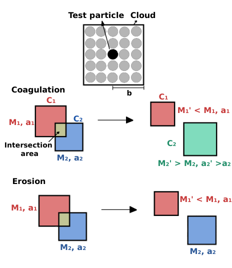
In a given region, we have a total amount of dust distributed over a given number of particles . In practice, is so large that it is unfeasible to follow the evolution of every single grain. Therefore, the common approach is to consider a finite number of test particles that represent a swarm of real particles. We shall suppose that the behavior of a test particle is representative of that of real particles, so they will have the same charge, velocity, and approximately the same position in space. For the implementation of the collision algorithm, we consider the computational test particles as the centroids of clouds of real particles uniformly distributed in a 2D domain (see Fig. 1 for an illustration). In order to avoid confusion, in the rest of this section we will use the term clouds for the test particles, and will reserve the word particle for referring to each of the real particles.
The size of the clouds is imposed by the properties of the particles they represent. If a cloud contains particles of radius , then its linear size is , where . This prescription is based on the assumption that the cloud has a squared shape, which corresponds to a uniform cartesian 2D distribution of the particles. Then, two clouds and will interact if the distance between them is , and the outcome of the interaction will be determined by their relative velocity :
- •
If , then the cloud of smaller particles loses mass (erosion).
- •
If , grain growth takes place (coagulation). In that case, we suppose that smaller particles get stuck into the larger ones, and the properties of both clouds will be modified.
The critical velocity depends on the grain material, and must be set by the user. In our simulations, we have adopted km s-1 for silicates and km s-1 for graphites as in HY09.
The properties of the clouds and will be modified as a function of the intersection area between them, . After an erosion event, only the cloud of smaller particles, let us say , loses mass: , where is the mass of the cloud and its area. For coagulation however, both clouds suffer complex modifications that have to be taken into account:
- •
The cloud of smaller particles () loses mass as when an erosion event takes place.
- •
Particles inside the cloud will experience growth. We suppose that there are and particles in the intersection area , and the smaller particles get stuck into the bigger ones. Hence, in the intersection area, the radius of the particles will be . The final radius of particles inside the cloud is computed through a weighted mean between the value inside the intersection area, , and outside of it, :
(1) - •
Since transfers mass to , it is to expect that momentum is also transferred during the coagulation process. If we denote by and the masses of particles inside the clouds and , then the velocity of the latter species is computed as:
(2) where is an efficiency factor that accounts for the fraction of energy transferred, and is the energy lost in creating the chemical bonds of the new particles. For , perfect coagulation takes place, while for all the energy is lost and erosion becomes the dominant outcome.
- •
Finally, the other particle properties such as charge (), Coulomb parameter , and cloud linear size () are set for both clouds according to their new properties. In particular, the grain charge is computed as in Paper I following Weingartner & Draine 2001a for several dust sizes under conditions typical of a molecular cloud envelope, and an analytical expression is then obtained of the form:
(3) where ) and () for silicate (graphite) grains11 1 This values have been obtained by fitting eq. 3 using the curve fitting tool cftool in Matlab (Matlab 2020).. This analytic expression is used inside the code to automatically update the particle charge. The Coulomb rate is then computed from the new dust charge as in Paper I, and the cloud size depends on the updated cloud mass.
In Fig. 1 we present an schematic view of both the coagulation and erosion processes for clarity.
According to this prescription, if we introduce several dust populations of radii , particles with may be formed, but those with that should be created after an erosion event will not be taken into account. The implications of this hypothesis on the physics are discussed later in Sec. V.
III Growth of a single-sized dust population
In Paper I, we showed that filaments of charged dust are able to form under conditions typical of a molecular cloud envelope ( K, cm-3, ionization fraction ); these parameters are very similar to those for the warm neutral medium (WNM), so this analysis is also valid for other diffuse regimes. However, in Paper I dust particles were not allowed to interact with each other and only suffered from the drag of neutral gas and magnetic fields.
We have first tested the performance of the collision model presented in the previous section using the results of Paper I as input data. With that purpose, we have selected seven regions where the dust-to-gas ratio is larger than the mean expected value for the diffuse ISM and for consistency, we keep the same names as in Paper I: H1, H2, H4, L1, L2, L4, and M1. In regions H1-H4, the gas density value is greater than 1; in regions L1-L4, it is lower than 1; and in region M1, the gas density reaches intermediate values. In all cases, conspicuous filaments of charged dust are formed aligned with the magnetic fields. We want to note that the computational domains for coagulation simulations are squared domains that contain the original regions, so their limits are slightly different as those in Paper I; the properties of these regions are summarized in Table 1.
| Region | Length | Resolution | ||||
|---|---|---|---|---|---|---|
| pc | px | g | g cm-3 | G | s | |
| H1 | 0.145 | 148 | 1.571 | 1.861 | 1.011 | 7.282 |
| H2 | 0.121 | 124 | 6.854 | 1.828 | 1.057 | 9.987 |
| H4 | 0.166 | 170 | 1.654 | 1.878 | 1.425 | 12.122 |
| L1 | 0.117 | 120 | 0.832 | 1.526 | 1.609 | 9.665 |
| L2 | 0.109 | 112 | 1.056 | 1.576 | 1.471 | 9.021 |
| L4 | 0.180 | 184 | 1.822 | 1.609 | 1.333 | 14.820 |
| M1 | 0.063 | 64 | 0.478 | 1.711 | 0.080 | 5.155 |
Note. — Regions selected from the turbulence simulation (Paper I) to study the performance of the dust coagulation algorithm. In all cases, they are taken to be squared regions of a fixed length as given in the table, and with a uniform resolution in x- and y- directions.
Given a region, we extract the gas properties and particle positions, and set them inside a new domain with normalized limits . The boundary conditions are chosen to be flow out to ensure that the divergence-free constraint holds . This implies that some mass of dust will be inevitably lost, but we will take this fact into account when discussing the performance of the algorithm. The initial dust population is homogeneous, with a common radius of m, a charge of , and an internal solid density g cm-3. As explained in Sec. II, the computational test particles have to be considered as the centroids of a squared cloud with linear size that depends on the dust content. At the initial stage, all the clouds have the same linear size, typically 1.4 times the pixel size; this means that the clouds span a region of pixels. The system is then left to evolve an arbitrary amount of time that differs from simulation to simulation. The final time is subjectively set following the condition that dust particles have moved enough to produce substantial coagulation, but they have not been completely swept away from the domain. A typical value is s ( Myr, see Table 1) that, when compared with the global simulation ( s), is roughly a of the total time. Hence, we expect that the phenomena observed in the simulations here presented are representative of the evolution of the global system (Paper I) at short time scales. Besides, if we compare this time with the typical lifetime of a molecular cloud (Hartmann et al. 2001, Myr,) it is evident that the timescales treated in this work are so small that we can consider that the final size distributions are representative for a molecular cloud at any stage of its evolution, provided that the ambient conditions (temperature, ionization fraction, magnetic field strength, and density) are maintained.
III.1 Evolution of the size distribution
Starting from single-sized dust grains, and given the fact that we are not allowing particles to decrease their size, we do not expect to retrieve a realistic size distribution of the type , (Mathis et al. 1977, hereafter MRN). In fact, attempts to fit the dust size distribution to a power law give very sharp values for ().
Globally, we find that a significant fraction of the dust population () have a final radius greater than the initial value of m, but only few of them (at most 2%) acquires a size greater or equal than twice the initial value (m). Besides, the growth also depends on the ambient conditions: particles that suffer from moderate growth (final sizes below m) are found all over the domain, but the largest particles are only created in high dust density regions with weak magnetic fields; this is logical since we are working with charged dust particles with large charge-to-mass ratios, so they are effectively accelerated by the Lorentz force. At high density regions, however, the magnetic field strength decreases and the dust grains are less accelerated. In every simulation we find one or two particles that are able to acquire very large sizes (from to m), and they are initially located in regions with a magnetic field strength lower than the mean.
Finally, we have qualitatively explored the possible influence of the morphology of the magnetic field in the observed dust growth. With that purpose, we have plotted the initial positions of all the particles that acquire a size greater than m () over the vectorial magnetic field, and also over the initial density field (see Fig. 2). In general, particle growth takes place inside the main dust filaments, parallel to the magnetic field lines, but the largest grains mentioned above form in high dust concentrations located inside magnetic field loops.
III.2 Dust mass loss
According to our model, there are two possible outcomes for a collision between two particles: one of them may grow, as we have already seen, or if their relative velocity is larger than the threshold, the less massive will suffer from erosion. This erosion is one of the main mechanisms for dust mass loss, and in practice we shall suppose that the mass lost after an erosion is actually converted into smaller dust grains that return to the gas phase and are not followed by our algorithm.
First, we have analyzed how many clouds lose dust mass but keep their original radius (m). Almost half of the clouds are eroded and for approximately 50% of them, the mass is reduced five orders of magnitude (see Fig. 2 for an illustration). This means that dust erosion is very likely to take place in molecular cloud envelopes, preventing the dust grains to acquire very large sizes, and increasing the abundance of small dust particles that interact very effectively with the ambient magnetic field.
We can further quantify the amount of dust that is lost in the interactions, i.e., the dust mass that is transferred to the smaller populations not tracked in our simulation. Comparing the number of clouds at the final stage of the simulation with the initial one, we can give a lower limit for the dust mass that has gone out of the domain, but that is not necessarily transferred to the small-sized population. Since at all the clouds have the same mass, we conclude that the amount of dust that has escaped the domain is of the total initial dust mass. This means that most of the mass, that is approximately a 40% of the initial one, is converted into small dust particles that return to a gaseous state.
IV Evolution of a realistic dust population
To complete the testing of the algorithm, we are interested in seeing how a realistic dust size distribution behaves. With that purpose, we have generated some mock dust samples for the regions studied in Sec. III and have evolved them up to the same time limit. Our objective is twofold: first, considering two independent dust populations (one composed of silicates and another one of graphite grains), study the variation in the power index of the size distribution; and second, taking the final dust size distributions, build the ultraviolet extinction curve and quantify the differences that arise due to dust coagulation and erosion events. In the next section (Sec. IV.1) we explain in detail how we have generated the mock samples for these tests, and the analysis of the size distribution is performed in Sec. IV.2. Finally, the study of the ultraviolet extinction curve is presented in Sec. IV.3.
IV.1 Generation of a mock sample
For a given region, we know the total amount of dust as listed in Table 1. Then, we suppose that the dust abundance is equally distributed between two populations, one of silicate grains with solid density g cm-3 and another one of graphite grains with g cm-3. Each population will be represented by ten dust families with sizes ranging from Å to m, logarithmically spaced to have a better sampling of the small end of the distribution: 5 nm, 7.7 nm, 11.9 nm, 18.4 nm, 28.4 nm, 43.9 nm, 67.9 nm, 104.8 nm, 161.9 nm, 250 nm. Since we are still working under conditions typical of a molecular cloud envelope, we compute the grain charges and Coulomb drag parameters for each dust family and composition as in Paper I (, ). Individual simulations with identical initial conditions are carried out for the silicate and graphite populations for simplicity, because our algorithm do not allow interaction between particles from different populations.
Independently on the dust abundance, for each region and material we generate 1000 clouds, a quantity imposed by computational restrictions, and consider a homogeneous sampling of the populations, which implies that 100 clouds of each size family are followed. Then, these clouds are distributed across the domain according to three criteria: particles with m should follow the original dust distribution from Paper I, those with will be placed according to the magnetic field strength, and those with will be generated according to the gas density; for m and m, we take a linear interpolation between the boundary values. Each mock cloud is generated in the center of a computational cell, and its velocity is also given as a function of the velocity field of the original dust distribution, the Alfvén velocity at cell-centers, and the gas velocity. A detailed explanation of the methods behind the random distribution of particles and the determination of their velocities can be found in Appendix A.
Finally, as we want this mock sample to be representative of a realistic dust size distribution, we distribute the dust mass among each population in order to satisfy the condition .
IV.2 Variations in the size distribution
We have studied separately the behavior of silicate and graphite grains, since differences are to be expected due to the smaller value of for graphites.
First, we analyzed the maximum achievable particle size. In general, silicate particles acquire radii up to m while graphite ones rarely grow beyond the upper boundary of m; this is consistent with the difference in the adopted values for . However, there are some exceptions: in region L4, there is one silicate grain that is able to grow up to m starting from a very small size ( nm). It is placed in a region that coincides with one of the filaments inside which dust grains are able to acquire sizes greater than m in the turbulent simulation (Sec. III). For the graphite grains, in region H2 there is one particle that grows up to m, while in L1 another one reaches m. In this case, however, both grains had an initial radius of m, and therefore they are not candidates to suffer erosion nor are accelerated by the magnetic fields (they move with the gas). Although these variations in the size distributions may seem relevant, we find very similar values when fitting the populations to a MRN power law (see Table 2). In concordance with the previous discussion, since silicate grains grow more efficiently than graphite particles, the power index of the former population is in general shallower than the latter one, but they are always of the order of .
Then, we have again quantified the percentage of mass lost by the system. We observe greater values than those of the turbulent case (Sec. III) where the mean was and approximately half of that mass was reconverted into smaller grains. This time, almost half of the mass disappears (see Table 2), but it is not distributed among the smaller population still present in the domain: practically 80% of the mass lost in this simulations is carried by very small particles of sizes 5 nm and 7 nm that rapidly drifts away from the domain. Since we are assuming a MRN-like initial size distribution, and we start with 100 particles for each radius, the smaller ones represent more mass than the larger ones. Besides, due to their very small sizes, their dynamics is governed by the charges, so they are effectively accelerated by the magnetic field, barely feel the gas, and move away. The effect is more pronounced for the graphite population because their charge parameters are slightly larger (see e.g. Draine 2004).
| Region | |||||||
|---|---|---|---|---|---|---|---|
| m | m | % | % | ||||
| H1 | 0.338 | 0.250 | -3.31 | -3.33 | 45.56 | 50.28 | 0.76 |
| H2 | 0.338 | 0.325 | -3.33 | -3.39 | 48.83 | 50.03 | 0.79 |
| H4 | 0.332 | 0.250 | -3.28 | -3.35 | 45.51 | 54.30 | 0.75 |
| L1 | 0.358 | 0.356 | -3.28 | -3.40 | 47.69 | 52.57 | 0.78 |
| L2 | 0.338 | 0.250 | -3.26 | -3.36 | 44.97 | 49.13 | 0.75 |
| L4 | 1.580 | 0.250 | -3.39 | -3.33 | 48.89 | 54.33 | 0.86 |
| M1 | 0.352 | 0.250 | -3.07 | -3.11 | 61.33 | 65.79 | 0.55 |
Note. — Maximum grain sizes, power index of the size distribution, and percentage of mass lost for silicate and graphite particles in the realistic simulations. The last column also shows the ratio between the FUV slope of the given curves and the initial MRN distribution.
IV.3 Variations in the UV extinction curve
Motivated by the deviations of the size distributions from the initial MRN shape, we have investigated the variations in the UV extinction curve that may arise due to grain growth in molecular cloud envelopes.
We follow the approach by Nozawa & Fukugita 2013 and compute the extinction curve as:
| (4) |
We take Å, m, and (Weingartner & Draine 2001b), where the index denotes the grain species (graphite or silicate) and cm2.5, cm2.5. The factor in equation 4 is the extinction efficiency factor for species , and is computed from the Mie theory using the optical constants22 2 The optical constants are available at Draine’s web page: https://www.astro.princeton.edu/~draine/dust/dust.diel.html. by Draine 2003. For graphite grains, we follow the standard 1/3 - 2/3 approach (, Weingartner & Draine 2001b; Nozawa & Fukugita 2013) and take the dielectric constants for particles of radius m.
For each region, we have built the extinction curve from equation 4 taking the values of listed in Table 2. We have further normalized the curve dividing by the extinction at 540 nm, which is the effective wavelength of the V band; an example is shown in Fig. 3. Using these normalized curves, we can now proceed to study the variations that arise at ultraviolet wavelengths due to grain growth.
As we mentioned in the introduction, there are two main features of the ultraviolet extinction curve that may vary due to grain growth. The most prominent one is the bump at 2175 Å (see Fig. 3), but other species apart from graphite and silicate grains should be considered for a realistic treatment, especially PAHs. However, we want to note that the very small graphite grains here considered have typical sizes similar to those of PAHs (of the order of a few nm). The main difference between graphite and PAHs is the nature of the chemical bonds (C-H in PAHs that are not present in graphite grains) that affect the dielectric constants and, in consequence, the shape of the UV bump. We will consider to include PAHs for future applications, but in this work we only aim to demonstrate the feasibility of our method, so we will restrict to the study of the FUV slope.
Comparing the values in Table 2 and the previous discussions on grain growth, we see that even a modest growth is translated into variations in the FUV slope of the order of . A depletion of small particles, which is translated into a shallower value of the power index of the size distribution , is always accompanied by a decrease of the FUV slope. Two regions stand out from the rest: L4 shows less conspicuous variations in the FUV slope, reaching a ratio ; actually, it is straightforward from values in Table 2 that this is the only region where the small graphite population has been less depleted than the silicate one. For M1 the effects are more acute: the value of the slope is reduced to a half of the MRN initial distribution due to grain escape in the simulations, but also due to the destruction of small particles during erosion events: only a 26% (silicate) and a 30.5% (graphite) of the lost mass is carried out by clouds that escape from the domain.
We have finally assessed which of the two populations (silicate or graphite) exerts more influence in the FUV extinction curve. With that purpose, we have used the values above presented together with those from mock populations with ranging from -3.0 to -3.5. As a general rule, for a given , there are not significant variations for the ratio for . However, we do observe significant variations when we fix the power index of the silicate size distribution and take . From this, we conclude that variations in the FUV slope of the UV extinction curve mainly arise from depletion of small graphite grains that return to the gas phase.
V Discussion and conclusions
In this work, we have studied the growth and erosion of interstellar dust grains under conditions typical of a molecular cloud envelope for different populations based on their evolution in 2D MHD simulations. Although our methodology is different from that in the common literature, we are going to compare our results with those by Yan et al. 2004 (hereafter YLD04) and by HY09 to determine the advantages of a direct dust modeling over a more general statistical (that may be regarded as 3D) approach. Both works consider charged dust grains accelerated by MHD turbulence in several phases of the ISM, and only take into account coagulation and shattering effects. We will discuss only the results for the WNM, since its properties are essentially the same as those adopted for our molecular cloud envelope model (see Sec. III).
YLD04 adopted a statistical description of MHD turbulence and damping processes to derive the grain velocities in the WNM and to estimate the critical size for silicate and carbonaceous grains in order to experience shattering and coagulation. According to their study, only grains larger than 0.2 m are able to suffer from shattering, while coagulation dominates for sizes lower than 0.02 m for silicates, and 0.04 m for carbonaceous grains. Similar results were reported by HY09, since they adopted YLD04’s velocities in order to evolve the grain size distribution. According to the latter work, the maximum grain size m cannot be superseded because either coagulation is not efficient enough or because they would be destroyed by shattering effects. However, the results presented in Sec. III and in Table 2 are not in agreement with that statement. In Table 3, we show the number of coagulation and erosion events for each simulation, as well as their mean duration time. Focusing on the turbulent simulation (Sec. III), it is straightforward that even a single-sized dust distribution may experience several coagulation and shattering events, but that their relative frequency differs. For regions H1, H2, and L2 coagulation and shattering are essentially balanced, while for H4, L1, L4, and M1 shattering dominates. However, since the mean and median interaction times are, in general, greater for shattering, the growing mechanisms for small dust particles are countered. These conclusions are further sustained by the results for the realistic size distributions considered in Sec. IV, since for them the shattering events are approximately five times more common than coagulation ones for both silicate and graphite grains. Nevertheless, we do observe growth for the silicate population due to the shorter timescales for erosion, while graphite grains barely supersede the maximum initial size due to the low potential barrier for erosion (lower value of ). We want to emphasize that we do not find any common trends between regions with the same gas density properties, i.e., coagulation and shattering are not governed by the gas but rather by the local morphology of the magnetic field.
| H1 | H2 | H4 | L1 | L2 | L4 | M1 | |
|---|---|---|---|---|---|---|---|
| Turbulent | simulation | ||||||
| Ncoag | 2664 | 895 | 1725 | 959 | 1635 | 1841 | 577 |
| ( s) | 0.71 | 1.45 | 1.42 | 1.39 | 1.70 | 2.24 | 0.23 |
| median ( s) | 11.3 | 29.9 | 2.05 | 6.44 | 4.51 | 3.21 | 1.17 |
| Nshat | 2680 | 803 | 2682 | 1341 | 1592 | 2695 | 1190 |
| ( s) | 1.11 | 1.78 | 1.25 | 1.18 | 1.26 | 1.70 | 0.82 |
| median ( s) | 1.21 | 3.53 | 1.16 | 1.40 | 1.70 | 1.16 | 0.59 |
| Realistic: | silicate | ||||||
| Ncoag | 174 | 144 | 149 | 160 | 179 | 154 | 221 |
| ( s) | 0.54 | 0.65 | 1.00 | 1.20 | 1.75 | 1.43 | 0.13 |
| median ( s) | 2.59 | 2.10 | 3.83 | 1.19 | 5.11 | 1.38 | 1.15 |
| Nshat | 772 | 878 | 805 | 883 | 979 | 873 | 1113 |
| ( s) | 7.57 | 4.09 | 5.07 | 4.74 | 4.03 | 6.22 | 6.00 |
| median ( s) | 5.24 | 1.60 | 1.76 | 1.42 | 1.19 | 2.31 | 9.71 |
| Realistic: | graphite | ||||||
| Ncoag | 165 | 144 | 136 | 155 | 189 | 150 | 167 |
| ( s) | 4.4 | 5.36 | 5.8 | 4.06 | 14.30 | 8.94 | 0.43 |
| median ( s) | 1.13 | 0.81 | 2.16 | 0.33 | 1.76 | 0.64 | 0.38 |
| Nshat | 908 | 943 | 1068 | 1039 | 1041 | 1024 | 1259 |
| ( s) | 8.23 | 5.13 | 6.94 | 5.99 | 6.56 | 9.48 | 7.25 |
| median ( s) | 3.42 | 1.91 | 2.07 | 1.28 | 1.32 | 1.80 | 7.44 |
The origin of the discrepancies between the work here presented and the ones by YLD04 and HY09 is very likely the fundamentally different followed approaches. While YLD04 and HY09 adopt a statistical 3D treatment for the grain’s velocities, we have studied dust interactions inside dense filaments formed in 2D MHD simulations, so the collision frequencies in our work are consequently greater because dust particles in our simulations are restricted to move in a plane; introducing one additional degree of freedom will likely reduce the collision rates, although the filamentary distribution will always favor grain-grain collisions. Then, when studying the general behavior of dust grains in a turbulent, generic ISM medium, YLD04 and HY09’s approaches may be considered a fair approximation, while for more specific studies, such as the one here presented, it may be useful to evolve a full realistic dust population submitted to the resolved forces of the gas and magnetic field.
Finally, we want to discuss the physical consequences of the hypothesis that the mass of dust lost in erosion events returns to the gas phase. When dealing with grain shattering, it is customary to assume that the dust mass is redistributed among the lower-sized population (see e.g. HY09). Although this approach is reasonable when evolving a dust size distribution, its implementation inside a framework where MHD codes are involved is not trivial. Trying to increase the small sized population of neighboring particles would inevitably introduce more restrictions to the algorithm difficult to justify and that would obscure the interpretation of the results. On the other hand, the assumption that the residual dust mass lost after a collision is converted into nanometer-sized particles that may return to the gas phase is more natural and easier to interpret.
To sum up, in this paper we have presented a new formulation to study the variations in the grain size distribution using a particle-in-cell code coupled with a MHD code. We have implemented this formulation in the MHD code Athena, and have used it to study the variations in the dust size distribution in a molecular cloud envelope and the expected variations in the FUV extinction curve. This work is very related to other recent attempts to include the evolution of the dust size distribution in MHD codes (McKinnon et al. 2018; Tamfal et al. 2018; Li & Mattsson 2020) but it is the only one that considers charged dust particles and that is designed for studies of the diffuse ISM. Currently, and up to the knowledge of the authors, the other numerical code that is considering the evolution of charged dust grains in the ISM is GIZMO (Hopkins 2015; Lee et al. 2017), but the public version only takes into account the interaction of dust particles with the gas and the magnetic fields.
Appendix A Generation of a mock sample
In order to generate the position and velocity of a mock cloud of particles with radius , , we make use of three probability matrices. We take as input data the matrix of magnetic field modulus in the region of interest , the matrix of the gas velocity modulus , and the matrix of dust mass from Paper I; we normalize these matrices so that the maximum value is 1. Then, for every cloud of particles with radius , the associated probability matrix is computed as follows:
| (A1) | |||
| (A2) |
where m is the adopted radius for the simulations in Paper I.
The probability matrix gives the 2D probability distribution of the clouds with radius . To assign a random position following this distribution, we marginalize over and retrieve the cumulative distribution function for the -position. Then, we take a random number from a uniform distribution and retrieve the associated -position from the cumulative distribution. Finally, the -position is generated in a similar manner, but this time the marginalized distribution is imposed by the -coordinate (it is a conditioned probability).
The velocity of the cloud is set based on its position in the grid. Since we are placing the clouds at the center of the computational cells, we can apply a linear relationship analogous to A1 and A2 but substituting the probability matrices , , and by the corresponding values of the velocities at that cell, , , and ; this is done on a component-by-component basis.
References
- Bakes & Tielens (1994) Bakes, E. L. O., & Tielens, A. G. G. M. 1994, ApJ, 427, 822, doi: 10.1086/174188
- Beitia-Antero & Gómez de Castro (2017) Beitia-Antero, L., & Gómez de Castro, A. I. 2017, MNRAS, 469, 2531, doi: 10.1093/mnras/stx881
- Beitia-Antero et al. (2020) Beitia-Antero, L., Gómez de Castro, A. I., & Vallejo, J. C. 2020, arXiv e-prints, arXiv:2008.13135. https://arxiv.org/abs/2008.13135
- Chapman & Wardle (2006) Chapman, J. F., & Wardle, M. 2006, MNRAS, 371, 513, doi: 10.1111/j.1365-2966.2006.10592.x
- Decleir et al. (2019) Decleir, M., De Looze, I., Boquien, M., et al. 2019, MNRAS, 486, 743, doi: 10.1093/mnras/stz805
- Dominik et al. (1989) Dominik, C., Gail, H. P., & Sedlmayr, E. 1989, A&A, 223, 227
- Draine (2003) Draine, B. T. 2003, ApJ, 598, 1026, doi: 10.1086/379123
- Draine (2004) Draine, B. T. 2004, in The Cold Universe, 213. https://arxiv.org/abs/astro-ph/0304488
- Draine & Salpeter (1979) Draine, B. T., & Salpeter, E. E. 1979, ApJ, 231, 77, doi: 10.1086/157165
- Dwek (1998) Dwek, E. 1998, ApJ, 501, 643, doi: 10.1086/305829
- Fitzpatrick & Massa (2007) Fitzpatrick, E. L., & Massa, D. 2007, ApJ, 663, 320, doi: 10.1086/518158
- Gómez de Castro et al. (2015) Gómez de Castro, A. I., López-Santiago, J., López-Martínez, F., et al. 2015, MNRAS, 449, 3867, doi: 10.1093/mnras/stv413
- Güttler et al. (2010) Güttler, C., Blum, J., Zsom, A., Ormel, C. W., & Dullemond, C. P. 2010, A&A, 513, A56, doi: 10.1051/0004-6361/200912852
- Hartmann et al. (2001) Hartmann, L., Ballesteros-Paredes, J., & Bergin, E. A. 2001, ApJ, 562, 852, doi: 10.1086/323863
- Hirashita & Nozawa (2013) Hirashita, H., & Nozawa, T. 2013, Earth, Planets, and Space, 65, 183, doi: 10.5047/eps.2012.03.003
- Hirashita & Yan (2009) Hirashita, H., & Yan, H. 2009, MNRAS, 394, 1061, doi: 10.1111/j.1365-2966.2009.14405.x
- Hollenbach & Salpeter (1971) Hollenbach, D., & Salpeter, E. E. 1971, ApJ, 163, 155, doi: 10.1086/150754
- Hopkins (2015) Hopkins, P. F. 2015, MNRAS, 450, 53, doi: 10.1093/mnras/stv195
- Iglesias-Groth (2004) Iglesias-Groth, S. 2004, ApJ, 608, L37, doi: 10.1086/422216
- Lee et al. (2017) Lee, H., Hopkins, P. F., & Squire, J. 2017, MNRAS, 469, 3532, doi: 10.1093/mnras/stx1097
- Li & Mattsson (2020) Li, X.-Y., & Mattsson, L. 2020, ApJ, 903, 148, doi: 10.3847/1538-4357/abb9ad
- Mathis et al. (1977) Mathis, J. S., Rumpl, W., & Nordsieck, K. H. 1977, ApJ, 217, 425, doi: 10.1086/155591
- Matlab (2020) Matlab. 2020, version 9.8.0.1451342 (R2020a) (Natick, Massachusetts: The MathWorks Inc.)
- McKinnon et al. (2018) McKinnon, R., Vogelsberger, M., Torrey, P., Marinacci, F., & Kannan, R. 2018, MNRAS, 478, 2851, doi: 10.1093/mnras/sty1248
- Nozawa & Fukugita (2013) Nozawa, T., & Fukugita, M. 2013, ApJ, 770, 27, doi: 10.1088/0004-637X/770/1/27
- Nozawa et al. (2003) Nozawa, T., Kozasa, T., Umeda, H., Maeda, K., & Nomoto, K. 2003, ApJ, 598, 785, doi: 10.1086/379011
- Pandey & Vladimirov (2019) Pandey, B. P., & Vladimirov, S. V. 2019, AJ, 157, 83, doi: 10.3847/1538-3881/aafc32
- Pilipp et al. (1987) Pilipp, W., Hartquist, T. W., Havnes, O., & Morfill, G. E. 1987, ApJ, 314, 341, doi: 10.1086/165064
- Prevot et al. (1984) Prevot, M. L., Lequeux, J., Maurice, E., Prevot, L., & Rocca-Volmerange, B. 1984, A&A, 132, 389
- Rai & Rastogi (2012) Rai, R. K., & Rastogi, S. 2012, MNRAS, 423, 2941, doi: 10.1111/j.1365-2966.2012.21109.x
- Stecher & Donn (1965) Stecher, T. P., & Donn, B. 1965, ApJ, 142, 1681, doi: 10.1086/148461
- Stone et al. (2008) Stone, J. M., Gardiner, T. A., Teuben, P., Hawley, J. F., & Simon, J. B. 2008, ApJS, 178, 137, doi: 10.1086/588755
- Tamfal et al. (2018) Tamfal, T., Dra̧żkowska, J., Mayer, L., & Surville, C. 2018, ApJ, 863, 97, doi: 10.3847/1538-4357/aad1f4
- Weingartner & Draine (2001a) Weingartner, J. C., & Draine, B. T. 2001a, ApJS, 134, 263, doi: 10.1086/320852
- Weingartner & Draine (2001b) —. 2001b, ApJ, 548, 296, doi: 10.1086/318651
- Witt et al. (1984) Witt, A. N., Bohlin, R. C., & Stecher, T. P. 1984, ApJ, 279, 698, doi: 10.1086/161934
- Yan et al. (2004) Yan, H., Lazarian, A., & Draine, B. T. 2004, ApJ, 616, 895, doi: 10.1086/425111
- Zhukovska et al. (2016) Zhukovska, S., Dobbs, C., Jenkins, E. B., & Klessen, R. S. 2016, ApJ, 831, 147, doi: 10.3847/0004-637X/831/2/147
- Zsom & Dullemond (2008) Zsom, A., & Dullemond, C. P. 2008, A&A, 489, 931, doi: 10.1051/0004-6361:200809921
- Zsom et al. (2010) Zsom, A., Ormel, C. W., Güttler, C., Blum, J., & Dullemond, C. P. 2010, A&A, 513, A57, doi: 10.1051/0004-6361/200912976