KLIEP is a classic method for density ratio estimation introduced in Sugiyama et al., 2008. Here we review the formulation of KLIEP because we deploy it as an example of the basic estimator of CDRE.

Let $r^{*}(x)=\frac{p(x)}{q(x)}$ be the (unknown) true density ratio, then $p(x)$ can be estimated by $\tilde{p}(x)=r(x)q(x)$, where $r^{*}(x)$ is modeled by $r(x)$. Hence, we can optimize $r(x)$ by minimizing the KL (KL)-divergence between $p(x)$ and $\tilde{p}(x)$ with respect to $r$:

where $r(x)$ should satisfy $r(x)>0$ and $\int r(x)q(x)dx=\int\tilde{p}(x)dx=1$. As the first term of the right-hand side in Equation 1 is constant w.r.t. $r(x)$, the empirical objective of optimizing $r(x)$ is as follows:

One convenient way of parameterizing $r(x)$ is by using a log-linear model with normalization, which then automatically satisfies the constraints in Equation 2:

where $\psi_{\beta}$ can be any deterministic function: we use a neural network as $\psi_{\beta}$ in our implementations, $\beta$ then representing parameters of the neural network.

The goal of CDRE is estimating density ratios between two distributions $r_{\tau,t}(x)=p_{\tau}(x)/q_{\tau,t}(x)$, where $\tau$ is the initial time index of starting tracing a distribution, $t$ denotes the current time index, and when $t>\tau$ the samples of $p_{\tau}(x)$ is unavailable. We refer to $p_{\tau}(x)$ as the original distribution and $q_{\tau,t}(x)$ as the dynamic distribution of $p_{\tau}(x)$. The dynamic distribution is assumed to be shifting away from its original distribution gradually over time. For example, let $\tau=1$, at $t=1$ we have access to samples of both $p_{\tau}$ and $q_{\tau,t}$, we can directly estimate $r_{\tau,t}$ by standard DRE, and when $t>1$, we have no access to samples of $p_{\tau}$ any longer, instead, we only have access to samples of $q_{\tau,t-1}$ and $q_{\tau,t}$. CDRE is proposed to estimate $r_{\tau,t}$ in such a situation. In addition, CDRE is able to estimate ratios of multiple pairs of the original and dynamic distributions by a single estimator. It avoids building separated estimators for tracing different original distributions in an application (e.g. seasonal data), which also fits the common setting of continual learning that we will introduce in the latter sections.

For simplicity of notation, we assume $\tau=1$ in the case of estimating density ratios between a single pair of original and dynamic distributions, and then omit $\tau$ in the basic formulations. Thus, the density function of the original distribution is denoted as $p(x)$ and its samples are unavailable when $t>1$. Similarly, $q_{t}(x)$ denotes the density function of the dynamic distribution at time $t$. The true density ratio $r^{*}_{t}(x)\triangleq p(x)/q_{t}(x)$ can be decomposed as follows:

where $r^{*}_{s_{t}}(x)\triangleq q_{t-1}(x)/q_{t}(x)$ represents the true density ratio between the two latest dynamic distributions. Using this decomposition we can estimate $p(x)/q_{t}(x)$ in an iterative manner without the need of storing samples from $p(x)$ when $t$ increases. The key point is that we can estimate $r^{*}_{t}(x)$ by estimating $r^{*}_{s_{t}}(x)$ when the estimation of $r^{*}_{t-1}(x)$ is known. In particular, it introduces one extra constraint:

Existing methods of DRE can be applied to estimating the initial ratio $r^{*}_{1}(x)=p(x)/q_{1}(x)$ and the latest ratio $r^{*}_{s_{t}}(x),\forall t>1$, as the basic ratio estimator of CDRE. Let $r_{t}(x)$ be the estimation of $r^{*}_{t}(x)$, where $r_{t-1}$ is already obtained, then the objective of CDRE can be expressed as:

where $J_{DRE}$ can be the objective of any method used for standard DRE, such as KLIEP (Sugiyama et al., 2008).

We now demonstrate how to instantiate CDRE by KLIEP, which we call CKLIEP (CKLIEP). Define $r_{t}(x),r_{t-1}(x)$ by the log-linear form as in Equation 3, let $N_{t}=N_{t-1}=N$ as the sample size of each distribution, then $r_{s_{t}}$ is as follows:

where $\beta_{t},\beta_{t-1}$ represent parameters of $r_{t}(x),r_{t-1}(x)$, respectively. When the constraint in Equation 6 is satisfied, we have the following equality by substituting Equation 7 into the constraint:

$r_{s_{t}}$ can then be rewritten in the same log-linear form of Equation 3 by substituting Equation 8 into Equation 7:

Now we can instantiate $J_{DRE}$ in Equation 6 by the objective of KLIEP (Equation 2) and adding the equality constraint (Equation 8) into the objective with a hyperparameter $\lambda_{c}$, which gives the objective of CKLIEP as the following:

where $\beta_{t-1}$ is the estimated parameter of $r_{t-1}(x)$ and hence a constant in the objective.

A concurrent work (Rhodes et al., 2020) has developed TRE (TRE) by the same consecutive decomposition in Equation 4 but with the following main differences: 1) the objective of TRE is to optimize a set of ratio estimators at the same time whereas CDRE only needs to optimize the latest ratio estimator; 2) TRErequires samples of all intermediate distributions as well as the original distribution, in contrast CDRE only requires samples of the two latest distributions.

Define $\hat{\beta}_{t}$ as the estimated parameter that satisfies:

Assume $\phi_{\beta_{t}}(x)$ (Equation 9) includes the correct function that there exists $\beta_{t}^{*}$ recovers the true ratio over the population:

Notations: $\leadsto$ and $\xrightarrow{P}$ mean convergence in distribution and convergence in probability, respectively.

Assumptions: We assume $q_{t}(x)$ and $q_{t-1}(x)$ are independent, $n_{t}=n_{t-1}=n$, where $n_{t}$ is the sample size of $q_{t}(x)$. Let $S_{t}$ be the support of $q_{t}$, we assume $S_{t-1}\subseteq S_{t}$ in all cases.

All proofs are provided in Appendix A. Corollary 1 shows that how the covariance matrix $\nu_{e}^{2}$ depends on the latest density ratio ($r^{*}_{s_{t}}$) when the distributions are from the exponential family. Since a smaller variance is better for convergence, we would prefer $r^{*}_{s_{t}}(x)=q_{t-1}(x)/q_{t}(x)$ is small, which means when $q_{t-1}(x)$ is large $q_{t}(x)$ should be also large. In this case, $r^{*}_{s_{t}}$ is less likely to explode and the variance of the estimated parameter would be likely confined. We demonstrate this by experiments with 1-D Gaussian distributions. We fix $q_{t-1}(x)=\mathcal{N}(0,1)$, setting $q_{t}(x)=\mathcal{N}(\mu_{t},1)$, where $\mu_{t}=\delta k,\delta=0.1,k\in\{0,1,\dots,20\}$. In this case, $T(x)=\{x,x^{2}\}$, $\beta_{t}=\{\beta_{t,1},\beta_{t,2}\}$, we display the diagonal of $\nu_{e}^{2}$ (variance of $\beta_{t,1},\beta_{t,2}$) in Figure 1. It is clear that when $q_{t}$ is farther to $q_{t-1}$, the variance is larger.

When $\beta_{t}=\beta^{*}_{t},n\rightarrow\infty$, we have $r_{t}(x)=r^{*}_{s_{t}}(x)r_{t-1}(x)$, then $\log r^{*}_{t}(x)-\log r_{t}(x)=\log r^{*}_{t-1}(x)-\log r_{t-1}(x)$, which means the error inherited from $r_{t-1}(x)$ will be the intrinsic error for estimating $r^{*}_{t}(x)$ due to the objective of CDRE is iterative. It indicates that smaller difference between each intermediate $q_{\tau}$ and $q_{\tau-1}$ ($\forall 1<\tau\leq t$) leads to a better estimation. We demonstrate in Section 4.2 that it is often the case in practice even when $\psi_{\beta^{*}_{t}}(x)$ is approximated by a non-linear model. Moreover, Figure 1 shows the variance of the estimation may grow rapidly when the difference between the two distributions exceeds a certain value. CKLIEP can prevent such an issue by ensuring the difference between any intermediate pairs of distributions is relatively small. We will demonstrate this in Section 4.2 as well.

Now we consider tracing multiple original distributions in CDRE, in which case a new pair of original and dynamic distributions will be added into the training process of the estimator at some time point. We refer to an original distribution as $p_{\tau}(x)$, where $\tau$ is the time index of starting tracing the original distribution. And samples of $p_{\tau}(x)$ are not available when $t>\tau$. Similarly, $q_{\tau,t}(x)$ denotes the dynamic distribution that corresponding to $p_{\tau}(x)$ at time $t$:

Where $r^{*}_{s_{\tau,t}}(x)={q_{\tau,t-1}(x)}/{q_{\tau,t}(x)}$. In this case, we optimize the estimator at time $t$ by an averaged objective:

where $\mathbb{T}$ is the set of time indices of adding original distributions, $|\mathbb{T}|$ is the size of $\mathbb{T}$. $\mathcal{L}_{t}(\beta_{t};\tau)$ is as the same as the loss function of a single original distribution ( Equation 10) for a given $\tau$. Further, $r_{s_{\tau,t}}(x)$ is also defined by the same form of Equation 9, the difference is that $\psi_{\beta_{t}}(x)$ becomes $\psi_{\beta_{t}}(x;\tau)$. In our implementation, we concatenate the time index $\tau$ to each data sample as the input of the ratio estimator. Thus, we can avoid learning separate ratio estimators for multiple original distributions. In addition, we set the output of $\psi_{\beta_{t}}(\cdot)$ as a $|\mathbb{T}|$-dimensional vector $\{o_{1},\dots,o_{i},\dots,o_{|\mathbb{T}|}\}$ where $o_{i}$ corresponds to the output of $\psi_{\beta_{t}}(x;\tau=\mathbb{T}_{i})$. Note that with CDRE we have the flexibility to extend the model architecture since the latest estimator function $\phi_{\beta_{t}}$ only needs the output of the previous estimator function $\psi_{\beta_{t-1}}$. This can be beneficial when the model capacity becomes a bottleneck of the performance.

The main concern of estimating density ratios stems from high-dimensional data. Several methods for dimensionality reduction in DRE have been introduced in (Sugiyama et al., 2012). A fundamental assumption of these methods is that the difference between two distributions can be confined to a subspace, which means ${p(z)}/{q(z)}={p(x)}/{q(x)}$ where $z$ is a lower-dimensional representation of $x$. This aims for exact density ratio estimation in a subspace but incurs a high computational cost. In most applications, a model (e.g. classifiers) is often trained upon a representation extractor, indicating a surrogate feature space of high-dimensional data can be used for the density ratio estimation in practice. For instance, most measurements of generative models estimate the difference between two distributions in a surrogate feature space, e.g., the inception feature defined for the IS (IS) (Salimans et al., 2016) is extracted by a neural network, and this method is also applied in many other measurements of generative models, e.g. FID (FID) (Heusel et al., 2017), KID (KID) (Bińkowski et al., 2018).

In prior work, a pre-trained classifier is often used to generate surrogate features of high-dimensional image data (e.g. inception features (Salimans et al., 2016)). However, it may be difficult to train such a classifier in online applications because: a) a homogeneous dataset for all unseen data or tasks may not be available in advance; b) labeled data may not be available in generative tasks. In order to cope with such circumstances, we introduce CVAE (CVAE) in a pipeline with CDRE. The loss function of CVAE is defined as the following:

where $q_{t}(z)=\mathcal{N}(\mu_{\theta_{t}}(x),\sigma_{\theta_{t}}(x))$, $\theta_{t}$ and $\vartheta_{t}$ denote parameters of the encoder and decoder of CVAE, respectively. $NLL$ is the negative log likelihood term as the same as in vanilla VAE (Kingma and Welling, 2013), the training data set includes samples of all dynamic distributions at the previous step ($q_{\tau,t-1}(x),\forall\tau<t$) and the samples of the current original distribution ($p_{t}(x)$). The KL-divergence term in the loss function serves a regularization term: the current encoder is expected to give similar $z$ for a similar $x$ comparing with the previous encoder. This term forces the consistency between inputs of the previous and current ratio estimators (i.e. inputs of $\psi_{\beta_{t-1}}$ and $\psi_{\beta_{t}}$ in Equation 10). CVAE can generate effective features without requiring labels or pre-training, nevertheless, other commonly used methods (e.g. pre-trained classifiers) are also applicable to CDRE.

We demonstrate that CDRE can be applied in backward covariate shift in which case the training set is shifting and the test set is from a previous distribution. It just swaps the situation of training and test set in common covariate shift (Sugiyama et al., 2008; Shimodaira, 2000). We assume a linear regression model defined as $\hat{y}=wx+b+\epsilon_{0}$, where the noise $\epsilon_{0}\sim\mathcal{N}(0,0.01)$. At time $\tau$, the training data $x\in D_{\tau}$ and $D_{\tau}$ is shifting away from $D_{1}$ gradually, where $\tau\in\{1,2,\dots,t\}$ and $t=10$ is the latest time index. Figure 2(a) displays the data distribution at time $\tau=1$ and $\tau=t$ in which we can see there exists notable difference between the two distributions. When the model is trained by $D_{t}$, it will not be able to accurately predict on test samples from $D_{1}$ unless we adjust the loss function by importance weights (i.e. density ratios) as in handling covariate shift:

Figure 2(b) shows the regression lines learned by the model at $\tau=t$ with and without the importance weights, where the weights ${q_{1}(x)}/{q_{t}(x)}$ are estimated by CKLIEP. We can see that the line learned with importance weights fits $D_{1}$ more accurately than the one without the weights. This enables the model to make reasonable predictions on test samples from $D_{1}$ when the training set of $D_{1}$ is not available.

By estimating density ratios, we can approximate $f$-divergences between two distributions:

where $x_{i}\sim q(x)$, $f(\cdot)$ is a convex function and $f(1)=0$. Thus, we can trace the distribution shifts by using CDRE to approximate the $f$-divergences between $p_{\tau}(x)$ and $q_{\tau,t}(x)$ in the online setting described in Section 2.2. In our implementations, we apply CKLIEP to instantiate CDRE and choose the KL-divergence (i.e. setting $f(r)=-\log(r)$) to instantiate $f$-divergences. We compare the performance of CKLIEP with KLIEP and true values using synthetic Gaussian data, where KLIEP has access to samples of all original distributions at all time. The sample size of each distribution in the experiments is 50000.

We first simulate the scenario of a single original distribution which is a 64-D Gaussian distribution $p(x)=\mathcal{N}(\mu_{0},\sigma_{0}^{2}I)$, where $\mu_{0}=0,\sigma_{0}=1$. At each time step, we shift the distribution by a constant change on its mean and variance: $q_{t}(x)=\mathcal{N}(\mu_{t},\sigma_{t}^{2}I),\mu_{t}=\mu_{0}+\Delta\mu*k,\sigma_{t}=\sigma_{0}-\Delta\sigma*k,\Delta\mu=\Delta\sigma=0.02$, $k$ is the number of time steps within one estimation interval. We set the total number of time steps to 20. We estimate $p(x)/q_{t}(x)$ by applying CKLIEP with two different time intervals: (1). CKLIEP-d1 is to estimate $p(x)/q_{t}(x)$ at each time step, i.e. $k=1$; (2). CKLIEP-d4 is to estimate $p(x)/q_{t}(x)$ at every four time steps, i.e. $k=4$. We compare the MAE of log ratios ($mae=\frac{1}{N}\sum_{n=1}^{N}|{\log r^{*}(x_{n})-\log\hat{r}(x_{n})}|$) estimated by CKLIEP and KLIEP in Figure 3(a), and compare the estimated KL-divergence with the true value in Figure 3(b). According to Corollary 1, the difference between $q_{t-1}(x)$ and $q_{t}(x)$ plays an important role in the estimation convergence, which explains why CKLIEP-d4 gets worse performance than CKLIEP-d1. KLIEP can be viewed as a special case of CKLIEP when $q_{t-1}(x)=p(x)$, so the difference between $p(x)$ and $q_{t}(x)$ is critical to its convergence as well. We can see that in Figures 3(a) and 3(b) KLIEP has become much worse at the last two steps due to the two distributions are too far away from each other and thus causes serious difficulties in its convergence with a fixed sample size.

We also simulate the scenario of multiple original distributions by 64-D Gaussian data: $p_{\tau}(x)=\mathcal{N}(\mu_{\tau},\sigma_{\tau}^{2}I)$, where $\tau\in\{1,2,\dots,10\},\mu_{\tau}=2\tau,\sigma_{\tau}=1$. We shift each joined original distribution ($p_{\tau}(x),\forall\tau<t$) by a constant change as the single pair scenario and set $k=1,\Delta\mu=\Delta\sigma=0.01$, and add a new original distribution ($p_{t}(x)$) at each time step. In Figure 3(c), we compare the averaged KL-divergences ($\bar{\mathcal{D}}=\frac{1}{t}\sum_{\tau=1}^{t}\mathcal{D}_{KL}(q_{\tau,t}||p_{\tau})$) estimated by CKLIEP and KLIEP with the true value. CKLIEP outperforms KLIEP when $t$ increases, which aligns with the scenario of a single original distribution.

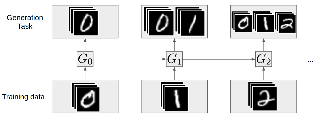
Evaluating a generative model in continual learning can be viewed as a special case of multiple original distributions of CDRE. A simplified scenario for generative models in continual learning is depicted in Figure 4, where the goal is to learn a generative model for one category (digit) per task while it still be able to generate samples of all previous categories. The training dataset of task $t$ consists of real samples of category $t$ and samples of task $1\cdots t-1$ generated by the previous model. The task index can be treated as the time index, the data distribution of the task $\tau$ can be viewed as a new original distribution $p_{\tau}(x)$ that added at time $\tau$, and its corresponding dynamic distribution $q_{\tau,t}(x)$ is the sample distribution generated by the model after trained on task $t$. The goal of generative models in continual learning is to make $q_{\tau,t}(x)$ as close to $p_{\tau}(x)$ as possible. In the sense of measuring the difference between $q_{\tau,t}(x)$ and $p_{\tau}(x)$, we can evaluate a generative model in continual learning by estimating the averaged $f$-divergences over all learned tasks:

Estimating $f$-divergences using density ratios has been well studied (Kanamori et al., 2011; Nguyen et al., 2010). Although the density ratio can also be estimated by the density functions of distributions, explicit density functions are often not available in practice. In the absence of prior work on evaluating generative models by $f$-divergences, we provide experimental results in the supplementary material for demonstrating differences between $f$-divergences, FID, KID, and PRD (PRD) (Sajjadi et al., 2018). Through these experiments, we show that $f$-divergences can be alternative measures of generative models and one may obtain richer criteria by them.

In our experiments, the evaluated GAN include WGAN (Arjovsky et al., 2017), WGAN-GP (Gulrajani et al., 2017), and two members of $f$-GANs (Nowozin et al., 2016): $f$-GAN-rvKL and $f$-GAN-JS, which instantiate the $f$-GAN by reverse KL and Jesen-Shannon divergences respectively. All GAN are tested as conditional GAN (Mirza and Osindero, 2014) using task indices as conditioners, and one task includes a single class of the data. We trained the GAN on Fashion-MNIST (Xiao et al., 2017). The sample size is 6000 for each class. More details of the experimental settings and the extra results with MNIST (LeCun et al., 2010) are provided in the supplementary material. We evaluate these GAN in continual learning by a few members of $f$-divergences which are estimated by CKLIEP, and compare the results with common measures FID, KID as used in static learning.

We deployed two feature generators in the experiments: 1) A classifier pre-trained on real samples of all classes, which is a CNN (CNN) and the extracted features are the activations of the last hidden layer (similar with inception feature); 2) A CVAE trained along with the procedure of continual learning, and the features are the output of the encoder. The dimension of features are 64 for both classifier and CVAE. We deployed the pre-trained classifier as the feature generator for FID,KID, and deployed the CVAE as the feature generator for CKLIEP in all experiments. Figure 5 compares the evaluations for the GAN by FID, KID, and four members of $f$-divergences (which are estimated by CKLIEP): KL, reverse KL, Jensen-Shannon, Hellinger. All these measures are the lower the better. We also display randomly chosen samples generated by those GAN in Figure 6 for a better understanding of the evaluations.

In general, all measurements give similar evaluations. For example, $f$-GAN-rvKL has the worst performance on all measures during the whole task sequence, whereas WGAN and WGAN-GP have similar performance on all measures. One main disagreement is that $f$-GAN-JS shows a decreasing trend on FID and KID but shows a slightly increasing trend on members of $f$-divergences. According to displayed samples of $f$-GAN-JS (Figure 6(c)), there is no notable improvement observed while $f$-GAN-JS learning more tasks, hence, the evaluations given by FID and KID are doubtful in this case. Moreover, KID also shows doubtful evaluations for WGAN and WGAN-GP. Visually, samples from WGAN and WGAN-GP (Figures 6(a) and 6(b)) are obviously losing fidelity while learning more tasks, which matches the increasing trend in all measures except KID. In principle, $f$-divergences may have different opinions with FID and KID because $f$-divergences are based on density ratios which may give more attention on parts with less probability mass (due to the ratio of two small values can be very large) whereas FID and KID are based on IPM (IPM) (Sriperumbudur et al., 2012) which focus on parts of the distribution with most probability mass. We illustrate this by a demo experiment in the supplementary material. All in all, these experimental results demonstrate that $f$-divergences estimated by CKLIEP can provide meaningful evaluations for generative models in continual learning.

References

- Arjovsky et al., (2017) Arjovsky, M., Chintala, S., and Bottou, L. (2017). Wasserstein generative adversarial networks. In International Conference on Machine Learning, pages 214–223.
- Bińkowski et al., (2018) Bińkowski, M., Sutherland, D. J., Arbel, M., and Gretton, A. (2018). Demystifying MMD GANs. In International Conference on Learning Representations (ICLR).
- Bouchikhi et al., (2018) Bouchikhi, I., Ferrari, A., Richard, C., Bourrier, A., and Bernot, M. (2018). Non-parametric online change-point detection with kernel lms by relative density ratio estimation. In 2018 IEEE Statistical Signal Processing Workshop (SSP), pages 538–542. IEEE.
- Gulrajani et al., (2017) Gulrajani, I., Ahmed, F., Arjovsky, M., Dumoulin, V., and Courville, A. C. (2017). Improved training of Wasserstein GANs. In Advances in Neural Information Processing Systems, pages 5767–5777.
- Heusel et al., (2017) Heusel, M., Ramsauer, H., Unterthiner, T., Nessler, B., and Hochreiter, S. (2017). GANs trained by a two time-scale update rule converge to a local Nash equilibrium. In Advances in Neural Information Processing Systems, pages 6626–6637.
- Kanamori et al., (2009) Kanamori, T., Hido, S., and Sugiyama, M. (2009). Efficient direct density ratio estimation for non-stationarity adaptation and outlier detection. In Advances in neural information processing systems, pages 809–816.
- Kanamori et al., (2011) Kanamori, T., Suzuki, T., and Sugiyama, M. (2011). -divergence estimation and two-sample homogeneity test under semiparametric density-ratio models. IEEE Transactions on Information Theory, 58(2):708–720.
- Karras et al., (2019) Karras, T., Laine, S., and Aila, T. (2019). A style-based generator architecture for generative adversarial networks. In Proceedings of the IEEE Conference on Computer Vision and Pattern Recognition, pages 4401–4410.
- Kawahara and Sugiyama, (2009) Kawahara, Y. and Sugiyama, M. (2009). Change-point detection in time-series data by direct density-ratio estimation. In Proceedings of the 2009 SIAM International Conference on Data Mining, pages 389–400. SIAM.
- Kingma and Welling, (2013) Kingma, D. P. and Welling, M. (2013). Auto-encoding variational Bayes. arXiv preprint arXiv:1312.6114.
- LeCun et al., (2010) LeCun, Y., Cortes, C., and Burges, C. (2010). MNIST handwritten digit database. AT&T Labs [Online]. Available: http://yann. lecun. com/exdb/mnist, 2:18.
- Lesort et al., (2018) Lesort, T., Caselles-Dupré, H., Garcia-Ortiz, M., Stoian, A., and Filliat, D. (2018). Generative models from the perspective of continual learning. arXiv preprint arXiv:1812.09111.
- Liu et al., (2013) Liu, S., Yamada, M., Collier, N., and Sugiyama, M. (2013). Change-point detection in time-series data by relative density-ratio estimation. Neural Networks, 43:72–83.
- McAllester and Stratos, (2020) McAllester, D. and Stratos, K. (2020). Formal limitations on the measurement of mutual information. In International Conference on Artificial Intelligence and Statistics, pages 875–884.
- Mirza and Osindero, (2014) Mirza, M. and Osindero, S. (2014). Conditional generative adversarial nets. arXiv preprint arXiv:1411.1784.
- Mohamed and Lakshminarayanan, (2016) Mohamed, S. and Lakshminarayanan, B. (2016). Learning in implicit generative models. arXiv preprint arXiv:1610.03483.
- Nguyen et al., (2010) Nguyen, X., Wainwright, M. J., and Jordan, M. I. (2010). Estimating divergence functionals and the likelihood ratio by convex risk minimization. IEEE Transactions on Information Theory, 56(11):5847–5861.
- Nowozin et al., (2016) Nowozin, S., Cseke, B., and Tomioka, R. (2016). f-GAN: Training generative neural samplers using variational divergence minimization. In Advances in Neural Information Processing Systems, pages 271–279.
- Parisi et al., (2019) Parisi, G. I., Kemker, R., Part, J. L., Kanan, C., and Wermter, S. (2019). Continual lifelong learning with neural networks: A review. Neural Networks.
- Rhodes et al., (2020) Rhodes, B., Xu, K., and Gutmann, M. U. (2020). Telescoping density-ratio estimation. NeurIPS.
- Sajjadi et al., (2018) Sajjadi, M. S., Bachem, O., Lucic, M., Bousquet, O., and Gelly, S. (2018). Assessing generative models via precision and recall. In Advances in Neural Information Processing Systems, pages 5228–5237.
- Salimans et al., (2016) Salimans, T., Goodfellow, I., Zaremba, W., Cheung, V., Radford, A., and Chen, X. (2016). Improved techniques for training GANs. In Advances in neural information processing systems, pages 2234–2242.
- Shalev-Shwartz et al., (2012) Shalev-Shwartz, S. et al. (2012). Online learning and online convex optimization. Foundations and Trends® in Machine Learning, 4(2):107–194.
- Shimodaira, (2000) Shimodaira, H. (2000). Improving predictive inference under covariate shift by weighting the log-likelihood function. Journal of statistical planning and inference, 90(2):227–244.
- Sriperumbudur et al., (2012) Sriperumbudur, B. K., Fukumizu, K., Gretton, A., Schölkopf, B., Lanckriet, G. R., et al. (2012). On the empirical estimation of integral probability metrics. Electronic Journal of Statistics, 6:1550–1599.
- Sugiyama et al., (2012) Sugiyama, M., Suzuki, T., and Kanamori, T. (2012). Density ratio estimation in machine learning. Cambridge University Press.
- Sugiyama et al., (2008) Sugiyama, M., Suzuki, T., Nakajima, S., Kashima, H., von Bünau, P., and Kawanabe, M. (2008). Direct importance estimation for covariate shift adaptation. Annals of the Institute of Statistical Mathematics, 60(4):699–746.
- Uehara et al., (2016) Uehara, M., Sato, I., Suzuki, M., Nakayama, K., and Matsuo, Y. (2016). Generative adversarial nets from a density ratio estimation perspective. arXiv preprint arXiv:1610.02920.
- Xiao et al., (2017) Xiao, H., Rasul, K., and Vollgraf, R. (2017). Fashion-MNIST: a novel image dataset for benchmarking machine learning algorithms.
- Xu et al., (2015) Xu, B., Wang, N., Chen, T., and Li, M. (2015). Empirical evaluation of rectified activations in convolutional network. arXiv preprint arXiv:1505.00853.
Appendix A Proof of asymptotic normality of CKLIEP
Define as the estimated parameter that satisfies: