跳到论文正文
W Papers独立论文阅读器 arXiv:2103.05243 论文正文 计算阅读时间 · 0%
引用这篇论文根据当前论文元数据生成,正式投稿前建议核对。


License: arXiv.org perpetual non-exclusive license
arXiv:2103.05243v3 [cs.LG] 07 Mar 2023

On the Generalization Power of
Overfitted Two-Layer Neural Tangent Kernel Models

Peizhong Ju Thanks: School of Electrical and Computer Engineering, Purdue University. Email: {jup,linx}@purdue.edu    Xiaojun Lin††footnotemark:    Ness B. Shroff Thanks: Department of ECE and CSE, The Ohio State University. Email: shroff.11@osu.edu
March 1, 2021
Abstract

In this paper, we study the generalization performance of min ℓ2\ell_{2}-norm overfitting solutions for the neural tangent kernel (NTK) model of a two-layer neural network with ReLU activation that has no bias term. We show that, depending on the ground-truth function, the test error of overfitted NTK models exhibits characteristics that are different from the “double-descent” of other overparameterized linear models with simple Fourier or Gaussian features. Specifically, for a class of learnable functions, we provide a new upper bound of the generalization error that approaches a small limiting value, even when the number of neurons pp approaches infinity. This limiting value further decreases with the number of training samples nn. For functions outside of this class, we provide a lower bound on the generalization error that does not diminish to zero even when nn and pp are both large.

1 Introduction

Recently, there is significant interest in understanding why overparameterized deep neural networks (DNNs) can still generalize well (Zhang et al. 2017; Advani et al. 2020), which seems to defy the classical understanding of bias-variance tradeoff in statistical learning (Bishop 2006; Hastie et al. 2009; Stein 1956; James & Stein 1992; LeCun et al. 1991; Tikhonov 1943). Towards this direction, a recent line of study has focused on overparameterized linear models (Belkin et al. 2018b; Belkin et al. 2019; Bartlett et al. 2020; Hastie et al. 2019; Muthukumar et al. 2019; Ju et al. 2020; Mei & Montanari 2019). For linear models with simple features (e.g., Gaussian features and Fourier features) (Belkin et al. 2018b; Belkin et al. 2019; Bartlett et al. 2020; Hastie et al. 2019; Muthukumar et al. 2019; Ju et al. 2020), an interesting “double-descent” phenomenon has been observed. Thus, there is a region where the number of model parameters (or linear features) is larger than the number of samples (and thus overfitting occurs), but the generalization error actually decreases with the number of features. However, linear models with these simple features are still quite different from nonlinear neural networks. Thus, although such results provide some hint why overparameterization and overfitting may be harmless, it is still unclear whether similar conclusions apply to neural networks.

In this paper, we are interested in linear models based on the neural tangent kernel (NTK) (Jacot et al. 2018), which can be viewed as a useful intermediate step towards modeling nonlinear neural networks. Essentially, NTK can be seen as a linear approximation of neural networks when the weights of the neurons do not change much. Indeed, Li & Liang 2018; Du et al. 2018 have shown that, for a wide and fully-connected two-layer neural network, both the neuron weights and their activation patterns do not change much after gradient descent (GD) training with a sufficiently small step size. As a result, such a shallow and wide neural network is approximately linear in the weights when there are a sufficient number of neurons, which suggests the utility of the NTK model.

Despite its linearity, however, characterizing the double descent of such a NTK model remains elusive. The work in Mei & Montanari 2019 also studies the double-descent of a linear version of two-layer neural network. It uses the so-called “random-feature” model, where the bottom-layer weights are random and fixed, and only the top-layer weights are trained. (In comparison, the NTK model for such a two-layer neural network corresponds to training only the bottom-layer weights.) However, the setting there requires the number of neurons, the number of samples, and the data dimension to all grow proportionally to infinity. In contrast, we are interested in the setting where the number of samples is given, and the number of neurons is allowed to be much larger than the number of samples. As a consequence of the different setting, in Mei & Montanari 2019 eventually only linear ground-truth functions can be learned. (Similar settings are also studied in d’Ascoli et al. 2020.) In contrast, we will show that far more complex functions can be learned in our setting. In a related work, Ghorbani et al. 2019 shows that both the random-feature model and the NTK model can approximate highly nonlinear ground-truth functions with a sufficient number of neurons. However, Ghorbani et al. 2019 mainly studies the expressiveness of the models, and therefore does not explain why overfitting solutions can still generalize well. To the best of our knowledge, our work is the first to characterize the double-descent of overfitting solutions based on the NTK model.

Specifically, in this paper we study the generalization error of the min ℓ2\ell_{2}-norm overfitting solution for a linear model based on the NTK of a two-layer neural network with ReLU activation that has no bias. Only the bottom-layer weights are trained. We are interested in min ℓ2\ell_{2}-norm overfitting solutions because gradient descent (GD) can be shown to converge to such solutions while driving the training error to zero (Zhang et al. 2017) (see also Section 2). Given a class of ground truth functions (see details in Section 3), which we refer to as “learnable functions,” our main result (Theorem 1) provides an upper bound on the generalization error of the min ℓ2\ell_{2}-norm overfitting solution for the two-layer NTK model with nn samples and pp neurons (for any finite pp larger than a polynomial function of nn). This upper bound confirms that the generalization error of the overfitting solution indeed exhibits descent in the overparameterized regime when pp increases. Further, our upper bound can also account for the noise in the training samples.

Our results reveal several important insights. First, we find that the (double) descent of the overfitted two-layer NTK model is drastically different from that of linear models with simple Gaussian or Fourier features (Belkin et al. 2018b; Belkin et al. 2019; Bartlett et al. 2020; Hastie et al. 2019; Muthukumar et al. 2019). Specifically, for linear models with simple features, when the number of features pp increases, the generalization error will eventually grow again and approach the so-called “null risk” (Hastie et al. 2019), which is the error of a trivial model that predicts zero. In contrast, for the class of learnable functions described earlier, the generalization error of the overfitted NTK model will continue to descend as pp grows to infinity, and will approach a limiting value that depends on the number of samples nn. Further, when there is no noise, this limiting value will decrease to zero as the number of samples nn increases. This difference is shown in Fig. 1(a). As pp increases, the test mean-square-error (MSE) of min-ℓ1\ell_{1} and min-ℓ2\ell_{2} overfitting solutions for Fourier features (blue and red curves) eventually grow back to the null risk (the black dashed line), even though they exhibit a descent at smaller pp. In contrast, the error of the overfitted NTK model continues to descend to a much lower level.

The second important insight is that the aforementioned behavior critically depends on the ground-truth function belonging to the class of “learnable functions.” Further, this class of learnable functions depend on the specific network architecture. For our NTK model (with RELU activation that has no bias), we precisely characterize this class of learnable functions. Specifically, for ground-truth functions that are outside the class of learnable functions, we show a lower bound on the generalization error that does not diminish to zero for any nn and pp (see Proposition 2 and Section 4). This difference is shown in Fig. 1(b), where we use an almost identical setting as Fig. 1(a), except a different ground-truth function. We can see in Fig. 1(b) that the test-error of the overfitted NTK model is always above the null risk and looks very different from that in Fig. 1(a). We note that whether certain functions are learnable or not critically depends on the specific structure of the NTK model, such as the choice of the activation unit. Recently, (Satpathi & Srikant 2021) shows that all polynomials can be learned by 2-layer NTK model with ReLU activation that has a bias term, provided that the number of neurons pp is sufficiently large. (See further discussions in Remark 2. However, (Satpathi & Srikant 2021) does not characterize the descent of generalization errors as pp increases.) This difference in the class of learnable functions between the two settings (ReLU with or without bias) also turns out to be consistent with the difference in the expressiveness of the neural networks. That is, shallow networks with biased-ReLU are known to be universal function approximators (Ji et al. 2019), while those without bias can only approximate the sum of linear functions and even functions (Ghorbani et al. 2019).

Refer to caption
Figure 1: The test mean-square-error(MSE) vs. the number of features/neurons pp for (a) learnable function and (b) not-learnable function when n=50n=50, d=2d=2, ‖ϵ‖22=0.01\|\bm{\epsilon}\|_{2}^{2}=0.01. The corresponding ground-truth are (a) f⁡(θ)=∑k∈{0,1,2,4}(sin⁡(k​θ)+cos⁡(k​θ))f(\theta)=\sum_{k\in\{0,1,2,4\}}(\sin(k\theta)+\cos(k\theta)), and (b) f⁡(θ)=∑k∈{3,5,7,9}(sin⁡(k​θ)+cos⁡(k​θ))f(\theta)=\sum_{k\in\{3,5,7,9\}}(\sin(k\theta)+\cos(k\theta)). (Note that in 2-dimension every input 𝒙\bm{x} on a unit circle can be represented by an angle θ∈[−π,π]\theta\in[-\pi,\pi]. See the end of Section 4.) Every curve is the average of 99 random simulation runs. For GD on the real neural network (NN), we use the step size 1/p1/\sqrt{p} and the number of training epochs is fixed at 20002000.

A closely related result to ours is the work in Arora et al. 2019, which characterizes the generalization performance of wide two-layer neural networks whose bottom-layer weights are trained by gradient descent (GD) to overfit the training samples. In particular, our class of learnable functions almost coincides with that of Arora et al. 2019. This is not surprising because, when the number of neurons is large, NTK becomes a close approximation of such two-layer neural networks. In that sense, the results in Arora et al. 2019 are even more faithful in following the GD dynamics of the original two-layer network. However, the advantage of the NTK model is that it is easier to analyze. In particular, the results in this paper can quantify how the generalization error descends with pp. In contrast, the results in Arora et al. 2019 provide only a generalization bound that is independent of pp (provided that pp is sufficiently large), but do not quantify the descent behavior as pp increases. Our numerical results in Fig. 1(a) suggest that, over a wide range of pp, the descent behavior of the NTK model (the green curve) matches well with that of two-layer neural networks trained by gradient descent (the cyan curve). Thus, we believe that our results also provide guidance for the latter model. The work in (Fiat et al. 2019) studies a different neural network architecture with gated ReLU, whose NTK model turns out to be the same as ours. However, similar to Arora et al. 2019, the result in Fiat et al. 2019 does not capture the speed of descent with respect to pp either. Second, Arora et al. 2019 only provides upper bounds on the generalization error. There is no corresponding lower bound to explain whether ground-truth functions outside a certain class are not learnable. Our result in Proposition 2 provides such a lower bound, and therefore more completely characterizes the class of learnable functions. (See further comparison in Remark 1 of Section 3 and Remark 3 of Section 5.) Another related work Allen-Zhu et al. 2019 also characterizes the class of learnable functions for two-layer and three-layer networks. However, Allen-Zhu et al. 2019 studies a training method that takes a new sample in every iteration, and thus does not overfit all training data. Finally, our paper studies generalization of NTK models for the regression setting, which is different from the classification setting that assumes a separability condition, e.g., in (Ji & Telgarsky 2019).

2 Problem Setup

We assume the following data model y=f⁡(𝒙)+ϵy=f(\bm{x})+\epsilon, with the input 𝒙∈ℝd\bm{x}\in\mathds{R}^{d}, the output y∈ℝy\in\mathds{R}, the noise ϵ∈ℝ\epsilon\in\mathds{R}, and f:ℝd↦ℝf:\ \mathds{R}^{d}\mapsto\mathds{R} denotes the ground-truth function. Let (𝐗i,yi)(\mathbf{X}_{i},\ y_{i}), i=1,2,⋯,ni=1,2,\cdots,n denote nn training samples. We collect them as 𝐗=[𝐗1𝐗2⋯𝐗n]∈ℝd×n\mathbf{X}=[\mathbf{X}_{1}\ \mathbf{X}_{2}\ \cdots\ \mathbf{X}_{n}]\in\mathds{R}^{d\times n}, 𝒚=[y1y2⋯yn]T∈ℝn\bm{y}=[y_{1}\ y_{2}\ \cdots\ y_{n}]^{T}\in\mathds{R}^{n}, ϵ=[ϵ1ϵ2⋯ϵn]T∈ℝn\bm{\epsilon}=[\epsilon_{1}\ \epsilon_{2}\ \cdots\ \epsilon_{n}]^{T}\in\mathds{R}^{n}, and 𝐅(𝐗)=[f(𝐗1)f(𝐗2)⋯f(𝐗n)]T∈ℝn\mathbf{F}(\mathbf{X})=[f(\mathbf{X}_{1})\ f(\mathbf{X}_{2})\ \cdots\ f(\mathbf{X}_{n})]^{T}\in\mathds{R}^{n}. Then, the training samples can be written as 𝒚=𝐅⁡(𝐗)+ϵ\bm{y}=\mathbf{F}(\mathbf{X})+\bm{\epsilon}. After training (to be described below), we denote the trained model by the function f^\hat{f}. Then, for any new test data 𝒙\bm{x}, we will calculate the test error by |f^​(𝒙)−f​(𝒙)||\hat{f}(\bm{x})-f(\bm{x})|, and the mean squared error (MSE) by 𝖤𝐱[f^​(𝐱)−f⁡(𝐱)]2\expectation_{\bm{x}}[\hat{f}(\bm{x})-f(\bm{x})]^{2}.

outputtop layer weights 𝒘\bm{w}input 𝒙=[x1​x2]T\bm{x}=[x_{1}\ x_{2}]^{T}bottom-layer weights 𝐕0\mathbf{V}_{0}hidden-layer: ReLU𝒘1\bm{w}_{1}𝒘3\bm{w}_{3}𝐕0​[1]\mathbf{V}_{0}[1]𝐕0​[2]\mathbf{V}_{0}[2]𝐕0​[3]\mathbf{V}_{0}[3]𝒘2\bm{w}_{2}x1x_{1}x2x_{2}
Figure 2: A two-layer neural network where d=2d=2, p=3p=3.

For training, consider a fully-connected two-layer neural network with pp neurons. Let 𝒘j∈ℝ\bm{w}_{j}\in\mathds{R} and 𝐕0​[j]∈ℝd\mathbf{V}_{0}[j]\in\mathds{R}^{d} denote the top-layer and bottom-layer weights, respectively, of the jj-th neuron, j=1,2,⋯,pj=1,2,\cdots,p (see Fig. 2). We collect them into 𝒘=[𝒘1𝒘2⋯𝒘p]T∈ℝp\bm{w}=[\bm{w}_{1}\ \bm{w}_{2}\ \cdots\ \bm{w}_{p}]^{T}\in\mathds{R}^{p}, and 𝐕0=[𝐕0[1]T𝐕0[2]T⋯𝐕0[p]T]T∈ℝd​p\mathbf{V}_{0}=[\mathbf{V}_{0}[1]^{T}\ \mathbf{V}_{0}[2]^{T}\ \cdots\ \mathbf{V}_{0}[p]^{T}]^{T}\in\mathds{R}^{dp} (a column vector with d​pdp elements). Note that with this notation, for any row or column vector 𝒗\bm{v} with d​pdp elements, 𝒗⁡[j]\bm{v}[j] denotes a (row/column) vector that consists of the (j​d+1)(jd+1)-th to (j​d+d)(jd+d)-th elements of 𝒗\bm{v}. We choose ReLU as the activation function for all neurons and there is no bias term in the ReLU activation function.

Now we are ready to introduce the NTK model (Jacot et al. 2018). We fix the top-layer weights 𝒘\bm{w}, and let the initial bottom-layer weights 𝐕0\mathbf{V}_{0} be randomly chosen. We then train only the bottom-layer weights. Let 𝐕0+Δ​𝐕¯\mathbf{V}_{0}+\overline{\Delta\mathbf{V}} denote the bottom-layer weights after training. Thus, the change of the output after training is

∑j=1p𝒘j𝟏{𝒙T(𝐕0[j]+Δ​𝐕¯[j])>0}⋅(𝐕0[j]+Δ​𝐕¯[j])T𝒙\displaystyle\sum_{j=1}^{p}\bm{w}_{j}\bm{1}_{\{\bm{x}^{T}(\mathbf{V}_{0}[j]+\overline{\Delta\mathbf{V}}[j])>0\}}\cdot(\mathbf{V}_{0}[j]+\overline{\Delta\mathbf{V}}[j])^{T}\bm{x}
−∑j=1p𝒘j𝟏{𝒙T𝐕0[j]>0}⋅𝐕0[j]T𝒙.\displaystyle-\sum_{j=1}^{p}\bm{w}_{j}\bm{1}_{\{\bm{x}^{T}\mathbf{V}_{0}[j]>0\}}\cdot\mathbf{V}_{0}[j]^{T}\bm{x}.

In the NTK model, one assumes that Δ​𝐕¯\overline{\Delta\mathbf{V}} is very small. As a result, 𝟏{𝒙T(𝐕0[j]+Δ​𝐕¯[j])>0}=𝟏{𝒙T𝐕0[j]>0}\bm{1}_{\{\bm{x}^{T}(\mathbf{V}_{0}[j]+\overline{\Delta\mathbf{V}}[j])>0\}}=\bm{1}_{\{\bm{x}^{T}\mathbf{V}_{0}[j]>0\}} for most 𝒙\bm{x}. Thus, the change of the output can be approximated by

∑j=1p𝒘j𝟏{𝒙T𝐕0[j]>0}⋅Δ​𝐕¯[j]T𝒙=𝒉𝐕0,𝒙Δ𝐕,\displaystyle\sum_{j=1}^{p}\bm{w}_{j}\bm{1}_{\{\bm{x}^{T}\mathbf{V}_{0}[j]>0\}}\cdot\overline{\Delta\mathbf{V}}[j]^{T}\bm{x}=\bm{h}_{\mathbf{V}_{0},\bm{x}}\Delta\mathbf{V},

where Δ​𝐕∈ℝd​p\Delta\mathbf{V}\in\mathds{R}^{dp} is given by Δ𝐕[j]:=𝒘jΔ​𝐕¯[j],j=1,2,⋯,p\Delta\mathbf{V}[j]\mathrel{\mathop{:}}=\bm{w}_{j}\overline{\Delta\mathbf{V}}[j],\ j=1,2,\cdots,p, and 𝒉𝐕0,𝒙∈ℝ1×(d​p)\bm{h}_{\mathbf{V}_{0},\bm{x}}\in\mathds{R}^{1\times(dp)} is given by

𝒉𝐕0,𝒙[j]:=𝟏{𝒙T𝐕0[j]>0}⋅𝒙T,j=1,2,⋯,p.\displaystyle\bm{h}_{\mathbf{V}_{0},\bm{x}}[j]\mathrel{\mathop{:}}=\bm{1}_{\{\bm{x}^{T}\mathbf{V}_{0}[j]>0\}}\cdot\bm{x}^{T},\ j=1,2,\cdots,p. (1)

In the NTK model, we assume that the output of the trained model is exactly given by Eq. (1), i.e.,

f^Δ​𝐕,𝐕0​(𝒙):=𝒉𝐕0,𝒙​Δ​𝐕.\displaystyle\hat{f}_{\Delta\mathbf{V},\mathbf{V}_{0}}(\bm{x})\mathrel{\mathop{:}}=\bm{h}_{\mathbf{V}_{0},\bm{x}}\Delta\mathbf{V}. (2)

In other words, the NTK model can be viewed as a linear approximation of the two-layer network when the change of the bottom-layer weights is small.

Define 𝐇∈ℝn×(d​p)\mathbf{H}\in\mathds{R}^{n\times(dp)} such that its ii-th row is 𝐇i:=𝒉𝐕0,𝐗i\mathbf{H}_{i}\mathrel{\mathop{:}}=\bm{h}_{\mathbf{V}_{0},\mathbf{X}_{i}}. Throughout the paper, we will focus on the following min-ℓ2\ell_{2}-norm overfitting solution

Δ​𝐕ℓ2:=arg​min𝐯⁡‖𝐯‖2, subject to ​𝐇​𝐯=𝐲.\displaystyle\Delta\mathbf{V}^{\ell_{2}}\mathrel{\mathop{:}}=\argmin_{\bm{v}}\|\bm{v}\|_{2},\text{ subject to }\mathbf{H}\bm{v}=\bm{y}.

Whenever Δ​𝐕ℓ2\Delta\mathbf{V}^{\ell_{2}} exists, it can be written in closed form as

Δ​𝐕ℓ2=𝐇T​(𝐇𝐇T)−1​𝒚.\displaystyle\Delta\mathbf{V}^{\ell_{2}}=\mathbf{H}^{T}(\mathbf{H}\mathbf{H}^{T})^{-1}\bm{y}. (3)

The reason that we are interested in Δ​𝐕ℓ2\Delta\mathbf{V}^{\ell_{2}} is that gradient descent (GD) or stochastic gradient descent (SGD) for the NTK model in Eq. (2) is known to converge to Δ​𝐕ℓ2\Delta\mathbf{V}^{\ell_{2}} (proven in Supplementary Material, Appendix B).

Using Eq. (2) and Eq. (3), the trained model is then

f^ℓ2​(𝒙):=𝒉𝐕0,𝒙​Δ​𝐕ℓ2.\displaystyle\hat{f}^{\ell_{2}}(\bm{x})\mathrel{\mathop{:}}=\bm{h}_{\mathbf{V}_{0},\bm{x}}\Delta\mathbf{V}^{\ell_{2}}. (4)

In the rest of the paper, we will study the generalization error of Eq. (4).

We collect some assumptions. Define the unit sphere in ℝd\mathds{R}^{d} as: 𝒮d−1:={𝒗∈ℝd|‖𝒗‖2=1}\mathcal{S}^{d-1}\mathrel{\mathop{:}}=\left\{\bm{v}\in\mathds{R}^{d}\ |\ \|\bm{v}\|_{2}=1\right\}. Let μ⁡(⋅)\mu(\cdot) denote the distribution of the input 𝒙\bm{x}. Without loss of generality, we make the following assumptions: (i) the inputs 𝒙\bm{x} are i.i.d. uniformly distributed in 𝒮d−1\mathcal{S}^{d-1}, and the initial weights 𝐕0​[j]\mathbf{V}_{0}[j]’s are i.i.d. uniformly distributed in all directions in ℝd\mathds{R}^{d}; (ii) p≥n/dp\geq n/d and d≥2d\geq 2; (iii) 𝐗i∦𝐗j\mathbf{X}_{i}\nparallel\mathbf{X}_{j} for any i≠ji\neq j, and 𝐕0​[k]∦𝐕0​[l]\mathbf{V}_{0}[k]\nparallel\mathbf{V}_{0}[l] for any k≠lk\neq l. We provide detailed justification of those assumptions in Supplementary Material, Appendix C.

3 Learnable Functions and Generalization Performance

We now show that the generalization performance of the overfitted NTK model in Eq. (4) crucially depends on the ground-truth function f⁡(⋅)f(\cdot), where good generalization performance only occurs when the ground-truth function is “learnable.” Below, we first describe a candidate class of ground-truth functions, and explain why they may correspond to the class of “learnable functions.” Then, we will give an upper-bound on the generalization performance for this class of ground-truth functions. Finally, we will give a lower-bound on the generalization performance when the ground-truth functions are outside of this class.

We first define a set ℱℓ2\mathcal{F}^{\ell_{2}} of ground-truth functions.

Definition 1.

ℱℓ2:={f=a.e.fg|fg(𝒙)=∫𝒮d−1𝒙T𝒛π−arccos⁡(𝒙T​𝒛)2​πg(𝒛)dμ(𝒛),∥g∥1<∞}\mathcal{F}^{\ell_{2}}\mathrel{\mathop{:}}=\big\{f\stackrel{{\scriptstyle\text{a.e.}}}{{=}}f_{g}\ \big|\ f_{g}(\bm{x})=\int_{\mathcal{S}^{d-1}}\bm{x}^{T}\bm{z}\frac{\pi-\arccos(\bm{x}^{T}\bm{z})}{2\pi}g(\bm{z})d\mu(\bm{z}),\ \|g\|_{1}<\infty\big\}.

Note that in Definition 1, =a.e.\stackrel{{\scriptstyle\text{a.e.}}}{{=}} means two functions equals almost everywhere, and ‖g‖1:=∫𝒮d−1|g⁡(𝒛)|​𝑑μ​(𝒛)\|g\|_{1}\mathrel{\mathop{:}}=\int_{\mathcal{S}^{d-1}}|g(\bm{z})|d\mu(\bm{z}). The function g⁡(𝒛)g(\bm{z}) may be any finite-value function in L1​(𝒮d−1↦ℝ)L^{1}(\mathcal{S}^{d-1}\mapsto\mathds{R}). Further, we also allow g⁡(𝒛)g(\bm{z}) to contain (as components) Dirac δ\delta-functions on 𝒮d−1\mathcal{S}^{d-1}. Note that a δ\delta-function δ𝒛0​(𝒛)\delta_{\bm{z}_{0}}(\bm{z}) has zero value for all 𝒛∈𝒮d−1∖{𝒛0}\bm{z}\in\mathcal{S}^{d-1}\setminus\{\bm{z}_{0}\}, but ‖δ𝒛0‖1:=∫𝒮d−1δ𝒛0​(𝒛)​𝑑μ​(𝒛)=1\|\delta_{\bm{z}_{0}}\|_{1}\mathrel{\mathop{:}}=\int_{\mathcal{S}^{d-1}}\delta_{\bm{z}_{0}}(\bm{z})d\mu(\bm{z})=1. Thus, the function g⁡(𝒛)g(\bm{z}) may contain any sum of δ\delta-functions and finite-value L1L^{1}-functions. 11 1 Alternatively, we can also interpret g⁡(𝒛)g(\bm{z}) as a signed measure (Rao & Rao 1983) on 𝒮d−1\mathcal{S}^{d-1}. Then, δ\delta-functions correspond to point masses, and the condition ‖g‖1<∞\|g\|_{1}<\infty implies that the corresponding unsigned version of the measure on 𝒮d−1\mathcal{S}^{d-1} is bounded.

To see why ℱℓ2\mathcal{F}^{\ell_{2}} may correspond to the class of learnable functions, we can first examine what the learned function f^ℓ2\hat{f}^{\ell_{2}} in Eq. (4) should look like. Recall that 𝐇T=[𝐇1T⋯𝐇nT]\mathbf{H}^{T}=[\mathbf{H}_{1}^{T}\ \cdots\ \mathbf{H}_{n}^{T}]. Thus, 𝒉𝐕0,𝒙​𝐇T=∑i=1n(𝒉𝐕0,𝒙​𝐇iT)​𝒆iT\bm{h}_{\mathbf{V}_{0},\bm{x}}\mathbf{H}^{T}=\sum_{i=1}^{n}(\bm{h}_{\mathbf{V}_{0},\bm{x}}\mathbf{H}_{i}^{T})\bm{e}_{i}^{T}, where 𝒆i∈ℝn\bm{e}_{i}\in\mathds{R}^{n} denotes the ii-th standard basis. Combining Eq. (3) and Eq. (4), we can see that the learned function in Eq. (4) is of the form

f^ℓ2​(𝒙)=\displaystyle\hat{f}^{\ell_{2}}(\bm{x})= 𝒉𝐕0,𝒙​𝐇T​(𝐇𝐇T)−1​𝒚\displaystyle\bm{h}_{\mathbf{V}_{0},\bm{x}}\mathbf{H}^{T}(\mathbf{H}\mathbf{H}^{T})^{-1}\bm{y}
=\displaystyle= ∑i=1n(1p​𝒉𝐕0,𝒙​𝐇iT)​p​𝒆iT​(𝐇𝐇T)−1​𝒚.\displaystyle\sum_{i=1}^{n}\left(\frac{1}{p}\bm{h}_{\mathbf{V}_{0},\bm{x}}\mathbf{H}_{i}^{T}\right)p\bm{e}_{i}^{T}(\mathbf{H}\mathbf{H}^{T})^{-1}\bm{y}. (5)

For all 𝒙,𝒛∈𝒮d−1\bm{x},\bm{z}\in\mathcal{S}^{d-1}, define 𝒞𝒛,𝒙𝐕0:={j∈{1,2,⋯,p}|𝒛T𝐕0[j]>0,𝒙T𝐕0[j]>0}\mathcal{C}_{\bm{z},\bm{x}}^{\mathbf{V}_{0}}\mathrel{\mathop{:}}=\{j\in\{1,2,\cdots,p\}\ |\ \bm{z}^{T}\mathbf{V}_{0}[j]>0,\bm{x}^{T}\mathbf{V}_{0}[j]>0\}, and its cardinality is given by

|𝒞𝒛,𝒙𝐕0|=∑j=1p𝟏{𝒛T​𝐕0​[j]>0,𝒙T​𝐕0​[j]>0}.\displaystyle\left|\mathcal{C}_{\bm{z},\bm{x}}^{\mathbf{V}_{0}}\right|=\sum_{j=1}^{p}\bm{1}_{\{\bm{z}^{T}\mathbf{V}_{0}[j]>0,\ \bm{x}^{T}\mathbf{V}_{0}[j]>0\}}. (6)

Then, using Eq. (1), we can show 1p​𝒉𝐕0,𝒙​𝐇iT=𝒙T​𝐗i​|𝒞𝐗i,𝒙𝐕0|p\frac{1}{p}\bm{h}_{\mathbf{V}_{0},\bm{x}}\mathbf{H}_{i}^{T}=\bm{x}^{T}\mathbf{X}_{i}\frac{|\mathcal{C}_{\mathbf{X}_{i},\bm{x}}^{\mathbf{V}_{0}}|}{p}. It is not hard to show that

|𝒞𝒛,𝒙𝐕0|p→Pπ−arccos⁡(𝒙T​𝒛)2​π, as ​p→∞.\displaystyle\frac{|\mathcal{C}_{\bm{z},\bm{x}}^{\mathbf{V}_{0}}|}{p}\stackrel{{\scriptstyle\text{P}}}{{\rightarrow}}\frac{\pi-\arccos(\bm{x}^{T}\bm{z})}{2\pi},\text{ as }p\to\infty. (7)

where →P\stackrel{{\scriptstyle\text{P}}}{{\rightarrow}} denotes converge in probability. (see Supplementary Material, Appendix D.5). Thus, if we let

g⁡(𝒛)=∑i=1np​𝒆iT​(𝐇𝐇T)−1​𝒚​δ𝐗i​(𝒛),\displaystyle g(\bm{z})=\sum_{i=1}^{n}p\bm{e}_{i}^{T}(\mathbf{H}\mathbf{H}^{T})^{-1}\bm{y}\delta_{\mathbf{X}_{i}}(\bm{z}), (8)

then as p→∞p\to\infty, Eq. (3) should approach a function in ℱℓ2\mathcal{F}^{\ell_{2}}. This explains why ℱℓ2\mathcal{F}^{\ell_{2}} is a candidate class of “learnable functions.” However, note that the above discussion only addresses the expressiveness of the model. It is still unclear whether any function in ℱℓ2\mathcal{F}^{\ell_{2}} can be learned with low generalization error. The following result provides the answer.

For some m∈[1,ln⁡nln⁡π2]m\in\left[1,\ \frac{\ln n}{\ln\frac{\pi}{2}}\right], define (recall that dd is the dimension of 𝒙\bm{x})

Jm​(n,d):=22​d+5.5​d0.5​d​n(2+1m)​(d−1).\displaystyle J_{m}(n,d)\mathrel{\mathop{:}}=2^{2d+5.5}d^{0.5d}n^{\left(2+\frac{1}{m}\right)(d-1)}. (9)
Theorem 1.

Assume a ground-truth function f=a.e.fg∈ℱℓ2f\stackrel{{\scriptstyle\text{a.e.}}}{{=}}f_{g}\in\mathcal{F}^{\ell_{2}} where ‖g‖∞<∞\|g\|_{\infty}<\infty22 2 The requirement of ‖g‖∞<∞\|g\|_{\infty}<\infty can be relaxed. We show in Supplementary Material, Appendix L that, even when gg is a δ\delta-function (so ‖g‖∞=∞\|g\|_{\infty}=\infty), we can still have a similar result of Eq. (10) but Term 1 will have a slower speed of decay O⁡(n−12​(d−1)​(1−1q))O(n^{-\frac{1}{2(d-1)}(1-\frac{1}{q})}) with respect to nn instead of O​(n−12​(1−1q))O(n^{-\frac{1}{2}}(1-\frac{1}{q})) shown in Eq. (10). Term 4 of Eq. (10) will also be different when gg is a δ\delta-function, but it still goes to zero when pp and nn are large. , n≥2n\geq 2, m∈[1,ln⁡nln⁡π2]m\in\left[1,\ \frac{\ln n}{\ln\frac{\pi}{2}}\right], d≤n4d\leq n^{4}, and p≥6​Jm​(n,d)​ln⁡(4​n1+1m)p\geq 6J_{m}(n,d)\ln\left(4n^{1+\frac{1}{m}}\right). Then, for any q∈[1,∞)q\in[1,\ \infty) and for almost every 𝐱∈𝒮d−1\bm{x}\in\mathcal{S}^{d-1}, we must have33 3 The notion 𝖯𝗋M\prob\limits_{M} in Eq. (10) emphasizes that randomness is in MM.

𝖯𝗋𝐕0,𝐗{|f^ℓ2(𝐱)−f(𝐱)|≥n−12​(1−1q)⏟Term 1\displaystyle\prob_{\mathbf{V}_{0},\mathbf{X}}\Big\{|\hat{f}^{\ell_{2}}(\bm{x})-f(\bm{x})|\geq\underbrace{n^{-\frac{1}{2}\left(1-\frac{1}{q}\right)}}_{\text{Term 1}}
+(1+Jm​(n,d)​n)​p−12​(1−1q)⏟Term 2+Jm​(n,d)​n​‖ϵ‖2⏟Term 3,\displaystyle+\underbrace{\left(1+\sqrt{J_{m}(n,d)n}\right)p^{-\frac{1}{2}\left(1-\frac{1}{q}\right)}}_{\text{Term 2}}+\underbrace{\sqrt{J_{m}(n,d)n}\|\bm{\epsilon}\|_{2}}_{\text{Term 3}},
 for all ϵ∈ℝn}≤2e2(exp⁡(−nq8​‖g‖∞2)⏟Term 4\displaystyle\quad\text{ for all }\bm{\epsilon}\in\mathds{R}^{n}\Big\}\leq 2e^{2}\bigg(\underbrace{\exp\left(-\frac{\sqrt[q]{n}}{8\|g\|_{\infty}^{2}}\right)}_{\text{Term 4}}
OPEN+exp⁡(−pq8​‖g‖12)⏟Term 5+exp⁡(−pq8​n​‖g‖12)⏟Term 6)+4nm⏟Term 7.\displaystyle+\underbrace{\exp\left(-\frac{\sqrt[q]{p}}{8\|g\|_{1}^{2}}\right)}_{\text{Term 5}}+\underbrace{\exp\left(-\frac{\sqrt[q]{p}}{8n\|g\|_{1}^{2}}\right)}_{\text{Term 6}}\bigg)+\underbrace{\frac{4}{\sqrt[m]{n}}}_{\text{Term 7}}. (10)

To interpret Theorem 1, we can first focus on the noiseless case, where ϵ\bm{\epsilon} and Term 3 are zero. If we fix nn and let p→∞p\to\infty, then Terms 2, 5, and 6 all approach zero. We can then conclude that, in the noiseless and heavily overparameterized setting (p→∞p\to\infty), the generalization error will converge to a small limiting value (Term 1) that depends only on nn. Further, this limiting value (Term 1) will converge to zero (so do Terms 4 and 7) as n→∞n\to\infty, i.e., when there are sufficiently many training samples. Finally, Theorem 1 holds even when there is noise.

The parameters of qq and mm can be tuned to make Eq. (10) sharper when nn and pp are large. For example, as we increase qq, Term 1 will approach n−0.5n^{-0.5}. Although a larger qq makes Terms 4, 5, and 6 bigger, as long as nn and pp are sufficiently large, those terms will still be close to 0. Similarly, if we increase mm, then Jm​(n,d)J_{m}(n,d) will approach the order of n2​(d−1)n^{2(d-1)}. As a result, Term 3 approaches the order of n2​d−0.5n^{2d-0.5} times ‖ϵ‖2\|\bm{\epsilon}\|_{2} and the requirement p≥6​Jm​(n,d)​ln⁡(4​n1+1m)p\geq 6J_{m}(n,d)\ln\left(4n^{1+\frac{1}{m}}\right) approaches the order of n2​(d−1)​ln⁡nn^{2(d-1)}\ln n.

Remark 1.

We note that Arora et al. 2019 shows that, for two-layer neural networks whose bottom-layer weights are trained by gradient descent, the generalization error for sufficiently large pp has the following upper bound: for any ζ>0\zeta>0,

𝖯𝗋{𝖤𝐱|f^(𝐱)−f(𝐱)|≤2​𝐲T​(𝐇∞)−1​𝐲n\displaystyle\prob\bigg\{\expectation_{\bm{x}}|\hat{f}(\bm{x})-f(\bm{x})|\leq\sqrt{\frac{2\bm{y}^{T}(\mathbf{H}^{\infty})^{-1}\bm{y}}{n}}
+O(log⁡nζ⋅min⁡𝖾𝗂𝗀⁡(𝐇∞)n)}≥1−ζ,\displaystyle+O\bigg(\sqrt{\frac{\log\frac{n}{\zeta\cdot\min\mathsf{eig}(\mathbf{H}^{\infty})}}{n}}\bigg)\bigg\}\geq 1-\zeta, (11)

where 𝐇∞=limp→∞(𝐇𝐇T/p)∈ℝn×n\mathbf{H}^{\infty}=\lim\limits_{p\to\infty}(\mathbf{H}\mathbf{H}^{T}/p)\in\mathds{R}^{n\times n}. For certain class of learnable functions (we will compare them with our ℱℓ2\mathcal{F}^{\ell_{2}} in Section 4), the quantity 𝒚T​(𝐇∞)−1​𝒚\bm{y}^{T}(\mathbf{H}^{\infty})^{-1}\bm{y} is bounded. Thus, 2​𝒚T​(𝐇∞)−1​𝒚n\sqrt{\frac{2\bm{y}^{T}(\mathbf{H}^{\infty})^{-1}\bm{y}}{n}} also decreases at the speed 1/n1/\sqrt{n}. The second O⁡(⋅)O(\cdot)-term in Eq. (1) contains the minimum eigenvalue of 𝐇∞\mathbf{H}^{\infty}, which decreases with nn. (Indeed, we show that this minimum eigenvalue is upper bounded by O⁡(n−1d−1)O(n^{-\frac{1}{d-1}}) in Supplementary Material, Appendix G.) Thus, Eq. (1) may decrease a little bit slower than 1/n1/\sqrt{n}, which is consistent with Term 1 in Eq. (10) (when qq is large). Note that the term 2​𝒚T​(𝐇∞)−1​𝒚2\bm{y}^{T}(\mathbf{H}^{\infty})^{-1}\bm{y} in Eq. (1) captures how the complexity of the ground-truth function affects the generalization error. Similarly, the norm of g⁡(⋅)g(\cdot) also captures the impact44 4 Although Term 1 in Eq. (10) in its current form does not depend on g⁡(⋅)g(\cdot), it is possible to modify our proof so that the norm of g⁡(⋅)g(\cdot) also enters Term 1. of the complexity of the ground-truth function in Eq. (10). However, we caution that the GD solution in Arora et al. 2019 is based on the original neural network, which is usually different from our min ℓ2\ell_{2}-norm solution based on the NTK model (even though they are close for very large pp). Thus, the two results may not be directly comparable.

Theorem 1 reveals several important insights on the generalization performance when the ground-truth function belongs to ℱℓ2\mathcal{F}^{\ell_{2}}.

(i) Descent in the overparameterized region: When pp increases, both sides of Eq. (10) decreases, suggesting that the test error of the overfitted NTK model decreases with pp. In Fig. 1(a), we choose a ground-truth function in ℱℓ2\mathcal{F}^{\ell_{2}} (we will explain why this function is in ℱℓ2\mathcal{F}^{\ell_{2}} later in Section 4). The test MSE of the aforementioned NTK model (green curve) confirms the overall trend55 5 This curve oscillates at the early stage when pp is small. We suspect it is because, at small pp, the convergence in Eq. (7) has not occurred yet, and thus the randomness in 𝐕0​[j]\mathbf{V}_{0}[j] makes the simulation results more volatile. of descent in the overparameterized region. We note that while Arora et al. 2019 provides a generalization error upper-bound for large pp (i.e., Eq. (1)), the upper bound there does not capture the dependency in pp and thus does not predict this descent.

More importantly, we note a significant difference between the descent in Theorem 1 and that of min ℓ2\ell_{2}-norm overfitting solutions for linear models with simple features (Belkin et al. 2018b; Belkin et al. 2019; Bartlett et al. 2020; Hastie et al. 2019; Muthukumar et al. 2019; Liao et al. 2020; Jacot et al. 2020). For example, for linear models with Gaussian features, we can obtain (see, e.g., Theorem 2 of Belkin et al. 2019):

MSE=‖f‖22​(1−np)+σ2​np−n−1, for p≥n+2\displaystyle\text{MSE}=\|f\|_{2}^{2}\left(1-\frac{n}{p}\right)+\frac{\sigma^{2}n}{p-n-1},\text{ for $p\geq n+2$} (12)

where σ2\sigma^{2} denotes the variance of the noise. If we let p→∞p\to\infty in Eq. (12), we can see that the MSE quickly approaches ‖f‖22\|f\|_{2}^{2}, which is referred to as the “null risk” (Hastie et al. 2019), i.e., the MSE of a model that predicts zero. Note that the null-risk is at the level of the signal, and thus is quite large. In contrast, as p→∞p\to\infty, the test error of the NTK model converges to a value determined by nn and ϵ\bm{\epsilon} (and is independent of the null risk). This difference is confirmed in Fig. 1(a), where the test MSE for the NTK model (green curve) is much lower than the null risk (the dashed line) when p→∞p\to\infty, while both the min ℓ2\ell_{2}-norm (the red curve) and the min ℓ1\ell_{1}-norm solutions (the blue curve) Ju et al. 2020 with Fourier features rise to the null risk when p→∞p\to\infty. Finally, note that the descent in Theorem 1 requires pp to increase much faster than nn. Specifically, to keep Term 2 in Eq. (10) small, it suffices to let pp increase a little bit faster than Ω⁡(n4​d−1)\Omega(n^{4d-1}). This is again quite different from the descent shown in Eq. (12) and in other related work using Fourier and Gaussian features (Liao et al. 2020; Jacot et al. 2020), where pp only needs to grow proportionally with nn.

(ii) Speed of the descent: Since Theorem 1 holds for finite pp, it also characterizes the speed of descent. In particular, Term 2 is proportional to p−12​(1−1q)p^{-\frac{1}{2}\left(1-\frac{1}{q}\right)}, which approaches 1/p1/\sqrt{p} when qq is large. Again, such a speed of descent is not captured in Arora et al. 2019. As we show in Fig. 1(a), the test error of the gradient descent solution under the original neural network (cyan curve) is usually quite close to that of the NTK model (green curve). Thus, our result provides useful guidance on how fast the generalization error descends with pp for such neural networks.

Refer to caption
Figure 3: The test MSE of the overfitted NTK model for the same ground-truth function as Fig. 1(a). (a) We fix n=50n=50 and increase pp for different noise level σ2\sigma^{2}. (b) We fix p=20000p=20000 and increase nn. All data points in this figure are the average of five random simulation runs.

(iii) The effect of noise: Term 3 in Eq. (10) characterizes the impact of the noise ϵ\bm{\epsilon}, which does not decrease or increase with pp. Notice that this is again very different from Eq. (12), i.e., results of min ℓ2\ell_{2}-norm overfitting solutions for simple features, where the noise term σ2​np−n−1→0\frac{\sigma^{2}n}{p-n-1}\to 0 when p→∞p\to\infty. We use Fig. 3(a) to validate this insight. In Fig. 3(a), we fix n=50n=50 and plot curves of test MSE of NTK overfitting solution as pp increases. We let the noise ϵi\epsilon_{i} in the ii-th training sample be i.i.d. Gaussian with zero mean and variance σ2\sigma^{2}. The green, red, and blue curves in Fig. 3(a) corresponds to the situation σ2=0\sigma^{2}=0, σ2=0.04\sigma^{2}=0.04, and σ2=0.16\sigma^{2}=0.16, respectively. We can see that all three curves become flat when pp is very large, and this phenomenon implies that the gap across different noise levels does not decrease when p→∞p\to\infty, which is in contrast to Eq. (12).

In Fig. 3(b), we instead fix p=20000p=20000, and increase nn). We plot the test MSE both for the noiseless setting (green curve) and for σ2=0.01\sigma^{2}=0.01 (red curve). The difference between the two curves (dashed blue curve) then captures the impact of noise, which is related to Term 3 in Eq. (10). Somewhat surprisingly, we find that the dashed blue curve is insensitive to nn, which suggests that Term 3 in Eq. (10) may have room for improvement.

In summary, we have shown that any ground-truth function in ℱℓ2\mathcal{F}^{\ell_{2}} leads to low generalization error for overfitted NTK models. It is then natural to ask what happens if the ground-truth function is not in ℱℓ2\mathcal{F}^{\ell_{2}}. Let ℱℓ2¯\overline{\mathcal{F}^{\ell_{2}}} denote the closure66 6 We consider the normed space of all functions in L2​(𝒮d−1↦ℝ)L^{2}(\mathcal{S}^{d-1}\mapsto\mathds{R}). Notice that although g⁡(𝒛)g(\bm{z}) in Definition 1 may not be in L2L^{2}, fgf_{g} is always in L2L^{2}. Specifically, fg​(𝒙)f_{g}(\bm{x}) is bounded for every 𝒙∈𝒮d−1\bm{x}\in\mathcal{S}^{d-1} when ‖g‖1<∞\|g\|_{1}<\infty. of ℱℓ2\mathcal{F}^{\ell_{2}}, and D⁡(f,ℱℓ2)D(f,\mathcal{F}^{\ell_{2}}) denotes the L2L^{2}-distance between ff and ℱℓ2\mathcal{F}^{\ell_{2}} (i.e., the infimum of the L2L^{2}-distance from ff to every function in ℱℓ2\mathcal{F}^{\ell_{2}}).

Proposition 2.

(i) For any given (𝐗,𝐲)(\mathbf{X},\bm{y}), there exists a function f^∞ℓ2∈ℱℓ2\hat{f}^{\ell_{2}}_{\infty}\in\mathcal{F}^{\ell_{2}} such that, uniformly over all 𝐱∈𝒮d−1\bm{x}\in\mathcal{S}^{d-1}, f^ℓ2​(𝐱)→Pf^∞ℓ2​(𝐱)\hat{f}^{\ell_{2}}(\bm{x})\stackrel{{\scriptstyle\text{P}}}{{\rightarrow}}\hat{f}^{\ell_{2}}_{\infty}(\bm{x}) as p→∞p\to\infty. (ii) Consequently, if the ground-truth function f∉ℱℓ2¯f\notin\overline{\mathcal{F}^{\ell_{2}}} (or equivalently, D⁡(f,ℱℓ2)>0D(f,\mathcal{F}^{\ell_{2}})>0), then the MSE of f^∞ℓ2\hat{f}^{\ell_{2}}_{\infty} (with respect to the ground-truth function ff) is at least D⁡(f,ℱℓ2)D(f,\mathcal{F}^{\ell_{2}}).

Intuitively, Proposition 2 (proven in Supplementary Material Appendix J) suggests that, if a ground-truth function is outside the closure of ℱℓ2\mathcal{F}^{\ell_{2}}, then no matter how large nn is, the test error of a NTK model with infinitely many neurons cannot be small (regardless whether or not the training samples contain noise). We validate this in Fig. 1(b), where a ground-truth function is chosen outside ℱℓ2¯\overline{\mathcal{F}^{\ell_{2}}}. The test MSE of NTK overfitting solutions (green curve) is above null risk (dashed black line) and thus is much higher compared with Fig. 1(a). We also plot the test MSE of the GD solution of the real neural network (cyan curve), which seems to show the same trend.

Comparing Theorem 1 and Proposition 2, we can clearly see that, all functions in ℱℓ2\mathcal{F}^{\ell_{2}} are learnable by the overfitted NTK model, and all functions not in ℱℓ2¯\overline{\mathcal{F}^{\ell_{2}}} are not.

4 What Exactly are the Functions in ℱℓ2\mathcal{F}^{\ell_{2}}?

Our expression for learnable functions in Definition 1 is still in an indirect form, i.e., through the unknown function g⁡(⋅)g(\cdot). In Arora et al. 2019, the authors show that all functions of the form (𝒙T​𝒂)l(\bm{x}^{T}\bm{a})^{l}, l∈{0,1,2,4,6,⋯}l\in\{0,1,2,4,6,\cdots\} are learnable by GD (assuming large pp and small step size), for a similar 2-layer network with ReLU activation that has no bias. In the following, we will show that our learnable functions in Definition 1 also have a similar form. Further, we can show that any functions of the form (𝒙T​𝒂)l(\bm{x}^{T}\bm{a})^{l}, l∈{3,5,7,⋯}l\in\{3,5,7,\cdots\} are not learnable. Our characterization uses an interesting connection to harmonics and filtering on 𝒮d−1\mathcal{S}^{d-1}, which may be of independent interest.

Towards this end, we first note that the integral form in Definition 1 can be viewed as a convolution on 𝒮d−1\mathcal{S}^{d-1} (denoted by ⊛\circledast). Specifically, for any fg∈ℱℓ2f_{g}\in\mathcal{F}^{\ell_{2}}, we can rewrite it as

fg​(𝒙)=g⊛h⁡(𝒙):=∫𝖲𝖮⁡(d)g⁡(𝐒​𝒆)​h​(𝐒−1​𝒙)​𝑑𝐒,\displaystyle f_{g}(\bm{x})=g\circledast h(\bm{x})\mathrel{\mathop{:}}=\int_{\mathsf{SO}(d)}g(\mathbf{S}\bm{e})h(\mathbf{S}^{-1}\bm{x})d\mathbf{S}, (13)
h⁡(𝒙):=𝒙T​𝒆​π−arccos⁡(𝒙T​𝒆)2​π,\displaystyle h(\bm{x})\mathrel{\mathop{:}}=\bm{x}^{T}\bm{e}\frac{\pi-\arccos(\bm{x}^{T}\bm{e})}{2\pi}, (14)

where 𝒆:=[0 0⋯ 0 1]T∈ℝd\bm{e}\mathrel{\mathop{:}}=[0\ 0\ \cdots\ 0\ 1]^{T}\in\mathds{R}^{d}, and 𝐒\mathbf{S} is a d×dd\times d orthogonal matrix that denotes a rotation in 𝒮d−1\mathcal{S}^{d-1}, chosen from the set 𝖲𝖮⁡(d)\mathsf{SO}(d) of all rotations. An important property of the convolution Eq. (13) is that it corresponds to multiplication in the frequency domain, similar to Fourier coefficients. To define such a transformation to the frequency domain, we use a set of hyper-spherical harmonics Ξ𝐊l\Xi_{\mathbf{K}}^{l} (Vilenkin 1968; Dokmanic & Petrinovic 2009) when d≥3d\geq 3, which forms an orthonormal basis for functions on 𝒮d−1\mathcal{S}^{d-1}. These harmonics are indexed by ll and 𝐊\mathbf{K}, where 𝐊=(k1,k2,⋯,kd−2)\mathbf{K}=(k_{1},k_{2},\cdots,k_{d-2}) and l=k0≥k1≥k2≥⋯≥kd−2≥0l=k_{0}\geq k_{1}\geq k_{2}\geq\cdots\geq k_{d-2}\geq 0 (those kik_{i}’s and ll are all non-negative integers). Any function f∈L2​(𝒮d−1↦ℝ)f\in L^{2}(\mathcal{S}^{d-1}\mapsto\mathds{R}) (including even δ\delta-functions (Li & Wong 2013)) can be decomposed uniquely into these harmonics, i.e., f⁡(𝒙)=∑l∑𝐊cf​(l,𝐊)​Ξ𝐊l​(𝒙)f(\bm{x})=\sum_{l}\sum_{\mathbf{K}}c_{f}(l,\mathbf{K})\Xi_{\mathbf{K}}^{l}(\bm{x}), where cf​(⋅,⋅)c_{f}(\cdot,\cdot) are projections of ff onto the basis function. In Eq. (13), let cg​(⋅,⋅)c_{g}(\cdot,\cdot) and ch​(⋅,⋅)c_{h}(\cdot,\cdot) denote the coefficients corresponding to the decompositions of gg and hh, respectively. Then, we must have (Dokmanic & Petrinovic 2009)

cfg​(l,𝐊)=Λ⋅cg​(l,𝐊)​ch​(l,𝟎),\displaystyle c_{f_{g}}(l,\mathbf{K})=\Lambda\cdot c_{g}(l,\mathbf{K})c_{h}(l,\bm{0}), (15)

where Λ\Lambda is some normalization constant. Notice that in Eq. (15), the coefficient for hh is ch​(l,𝟎)c_{h}(l,\bm{0}) instead of ch​(l,𝐊)c_{h}(l,\mathbf{K}), which is due to the intrinsic rotational symmetry of such convolution (Dokmanic & Petrinovic 2009).

The above decomposition has an interesting “filtering” interpretation as follows. We can regard the function hh as a “filter” or “channel,” while the function gg as a transmitted “signal.” Then, the function fgf_{g} in Eq. (13) and Eq. (15) can be regarded as the received signal after gg goes through the channel/filter hh. Therefore, when coefficient ch​(l,𝟎)c_{h}(l,\bm{0}) of hh is non-zero, then the corresponding coefficient cfg​(l,𝐊)c_{f_{g}}(l,\mathbf{K}) for fgf_{g} can be any value (because we can arbitrarily choose gg). In contrast, if a coefficient ch​(l,𝟎)c_{h}(l,\bm{0}) of hh is zero, then the corresponding coefficient cfg​(l,𝐊)c_{f_{g}}(l,\mathbf{K}) for fgf_{g} must also be zero for all 𝐊\mathbf{K}.

Ideally, if hh contains all “frequencies,” i.e., all coefficients ch​(l,𝟎)c_{h}(l,\bm{0}) are non-zero, then fgf_{g} can also contain all “frequencies,” which means that ℱℓ2\mathcal{F}^{\ell_{2}} can contain almost all functions. Unfortunately, this is not true for the function hh given in Eq. (14). Specifically, using the harmonics defined in Dokmanic & Petrinovic 2009, the basis Ξ𝟎l\Xi_{\bm{0}}^{l} for (l,𝟎)(l,\bm{0}) turns out to have the form

Ξ𝟎l​(𝒙)=∑k=0⌊l2⌋(−1)k⋅al,k⋅(𝒙T​𝒆)l−2​k,\displaystyle\Xi_{\bm{0}}^{l}(\bm{x})=\sum_{k=0}^{\lfloor\frac{l}{2}\rfloor}(-1)^{k}\cdot a_{l,k}\cdot(\bm{x}^{T}\bm{e})^{l-2k}, (16)

where al,ka_{l,k} are positive constants. Note that the expression Eq. (16) contains either only even powers of 𝒙T​𝒆\bm{x}^{T}\bm{e} (if ll is even) or odd powers of 𝒙T​𝒆\bm{x}^{T}\bm{e} (if ll is odd). Then, for the function hh in Eq. (14), we have the following proposition (proven in Supplementary Material, Appendix K.4). We note that (Basri et al. 2019) has a similar harmonics analysis, where the expression of ch​(l,𝟎)c_{h}(l,\bm{0}) is given. However, it is not obvious that the expression of ch​(l,𝟎)c_{h}(l,\bm{0}) for all l=0,1,2,4,6,⋯l=0,1,2,4,6,\cdots given in (Basri et al. 2019) must be non-zero, which is made clear by Proposition 3 as follows.

Proposition 3.

ch​(l,𝟎)c_{h}(l,\bm{0}) is zero for l=3,5,7,⋯l=3,5,7,\cdots and is non-zero for l=0,1,2,4,6,⋯l=0,1,2,4,6,\cdots.

We are now ready to characterize what functions are in ℱℓ2\mathcal{F}^{\ell_{2}}. By the form of Eq. (16), for any non-negative integer kk, any even power (𝒙T​𝒆)2​k(\bm{x}^{T}\bm{e})^{2k} is a linear combination of Ξ𝟎0,Ξ𝟎2,⋯,Ξ𝟎2​k\Xi_{\bm{0}}^{0},\Xi_{\bm{0}}^{2},\cdots,\Xi_{\bm{0}}^{2k}, and any odd power (𝒙T​𝒆)2​k+1(\bm{x}^{T}\bm{e})^{2k+1} is a linear combination of Ξ𝟎1,Ξ𝟎3,⋯,Ξ𝟎2​k+1\Xi_{\bm{0}}^{1},\Xi_{\bm{0}}^{3},\cdots,\Xi_{\bm{0}}^{2k+1}. By Proposition 3, we thus conclude that any function fg​(𝒙)=(𝒙T​𝒆)lf_{g}(\bm{x})=(\bm{x}^{T}\bm{e})^{l} where l∈{0,1,2,4,6,⋯}l\in\{0,1,2,4,6,\cdots\} can be written in the form of Eq. (15) in the frequency domain, and thus are in ℱℓ2\mathcal{F}^{\ell_{2}}. In contrast, any function f⁡(𝒙)=(𝒙T​𝒆)lf(\bm{x})=(\bm{x}^{T}\bm{e})^{l} where l∈{3,5,7,⋯}l\in\{3,5,7,\cdots\} cannot be written in the form of Eq. (15), and are thus not in ℱℓ2\mathcal{F}^{\ell_{2}}. Further, the ℓ2\ell_{2}-norm of any latter function will also be equal to its distance to ℱ∞\mathcal{F}^{\infty}. Therefore, the generalization-error lower-bound in Proposition 2 will apply (with D⁡(f,ℱℓ2)=‖f‖2D(f,\mathcal{F}^{\ell_{2}})=\|f\|_{2}). Finally, by Eq. (13), ℱℓ2\mathcal{F}^{\ell_{2}} is invariant under rotation and finite linear summation. Therefore, any finite sum of (𝒙T​𝒂)l(\bm{x}^{T}\bm{a})^{l}, l=0,1,2,4,6,⋯l=0,1,2,4,6,\cdots must also belong to ℱℓ2\mathcal{F}^{\ell_{2}}.

For the special case of d=2d=2, the input 𝒙\bm{x} corresponds to an angle θ∈[−π,π]\theta\in[-\pi,\pi], and the above-mentioned harmonics become Fourier series sin⁡(k​θ)\sin(k\theta) and cos⁡(k​θ)\cos(k\theta), k=0,1,⋯k=0,1,\cdots. We can then get similar results that frequencies of k∈{0,1,2,4,6,⋯}k\in\{0,1,2,4,6,\cdots\} are learnable (while others are not), which explains the learnable and not-learnable functions in Fig. 1. Details can be found in Supplementary Material, Appendix K.5.

Remark 2.

We caution that the above claim on non-learnable functions critically depends on the network architecture. That is, we assume throughout this paper that the ReLU activation has no bias. It is known from an expressiveness point of view that, using ReLU without bias, a shallow network can only approximate the sum of linear functions and even functions (Ghorbani et al. 2019). Thus, it is not surprising that other odd-power (but non-linear) polynomials cannot be learned. In contrast, by adding a bias, a shallow network using ReLU becomes a universal approximator (Ji et al. 2019). The recent work of Satpathi & Srikant 2021 shows that polynomials with all powers can be learned by the corresponding 2-layer NTK model. These results are consistent with ours because a ReLU activation function operating on 𝒙~∈ℝd−1\tilde{\bm{x}}\in\mathds{R}^{d-1} with a bias can be equivalently viewed as one operating on a dd-dimension input (with the last-dimension being fixed at 1/d1/\sqrt{d}) but with no bias. Even though only a subset of functions are learnable in the dd-dimension space, when projected into a (d−1)(d-1)-dimension subspace, they may already span all functions. For example, one could write (𝒙T​𝒂)3(\bm{x}^{T}\bm{a})^{3} as a linear combination of (OPEN[𝒙~1/d]T​𝒃i)li\begin{bmatrix}\tilde{\bm{x}}\\ 1/\sqrt{d}\end{bmatrix}^{T}\bm{b}_{i})^{l_{i}}, where i∈{1,2,⋯,5}i\in\{1,2,\cdots,5\}, [l1,⋯,l5]=[4,4,2,1,0][l_{1},\cdots,l_{5}]=[4,4,2,1,0], and 𝒃i∈ℝd\bm{b}_{i}\in\mathds{R}^{d} depends only on 𝒂\bm{a}. (See Supplementary Material, Appendix K.6 for details.) It remains an interesting question whether similar difference arises for other network architectures (e.g., with more than 2 layers).

5 Proof Sketch of Theorem 1

In this section, we sketch the key steps to prove Theorem 1. Starting from Eq. (3), we have

Δ​𝐕ℓ2=𝐇T​(𝐇𝐇T)−1​(𝐅⁡(𝐗)+ϵ).\displaystyle\Delta\mathbf{V}^{\ell_{2}}=\mathbf{H}^{T}(\mathbf{H}\mathbf{H}^{T})^{-1}\left(\mathbf{F}(\mathbf{X})+\bm{\epsilon}\right). (17)

For the learned model f^ℓ2​(𝒙)=𝒉𝐕0,𝒙​Δ​𝐕ℓ2\hat{f}^{\ell_{2}}(\bm{x})=\bm{h}_{\mathbf{V}_{0},\bm{x}}\Delta\mathbf{V}^{\ell_{2}} given in Eq. (4), the error for any test input 𝒙\bm{x} is then

f^ℓ2​(𝒙)−f​(𝒙)=\displaystyle\hat{f}^{\ell_{2}}(\bm{x})-f(\bm{x})= (𝒉𝐕0,𝒙​𝐇T​(𝐇𝐇T)−1​𝐅​(𝐗)−f⁡(𝒙))\displaystyle\left(\bm{h}_{\mathbf{V}_{0},\bm{x}}\mathbf{H}^{T}(\mathbf{H}\mathbf{H}^{T})^{-1}\mathbf{F}(\mathbf{X})-f(\bm{x})\right)
+𝒉𝐕0,𝒙​𝐇T​(𝐇𝐇T)−1​ϵ.\displaystyle+\bm{h}_{\mathbf{V}_{0},\bm{x}}\mathbf{H}^{T}(\mathbf{H}\mathbf{H}^{T})^{-1}\bm{\epsilon}. (18)

In the classical “bias-variance” analysis with respect to MSE (Belkin et al. 2018a), the first term on the right-hand-side of Eq. (5) contributes to the bias and the second term contributes to the variance. We first quantify the second term (i.e., the variance) in the following proposition.

Proposition 4.

For any n≥2n\geq 2, m∈[1,ln⁡nln⁡π2]m\in\left[1,\ \frac{\ln n}{\ln\frac{\pi}{2}}\right], d≤n4d\leq n^{4}, if p≥6​Jm​(n,d)​ln⁡(4​n1+1m)p\geq 6J_{m}(n,d)\ln\left(4n^{1+\frac{1}{m}}\right), we must have 𝖯𝗋𝐗,𝐕0{|𝐡𝐕0,𝐱​𝐇T​(𝐇𝐇T)−1​ϵ|≤Jm​(n,d)​n​‖ϵ‖2, for all ​ϵ∈ℝn}≥1−2nm\prob\limits_{\mathbf{X},\mathbf{V}_{0}}\big\{|\bm{h}_{\mathbf{V}_{0},\bm{x}}\mathbf{H}^{T}(\mathbf{H}\mathbf{H}^{T})^{-1}\bm{\epsilon}|\leq\sqrt{J_{m}(n,d)n}\|\bm{\epsilon}\|_{2},\text{ for all }\bm{\epsilon}\in\mathds{R}^{n}\big\}\geq 1-\frac{2}{\sqrt[m]{n}}.

The proof is in Supplementary Material Appendix F. Proposition 4 implies that, for fixed nn and dd, when p→∞p\to\infty, with high probability the variance will not exceed a certain factor of the noise ‖ϵ‖2\|\bm{\epsilon}\|_{2}. In other words, the variance will not go to infinity when p→∞p\to\infty. The main step in the proof is to lower bound min⁡𝖾𝗂𝗀⁡(𝐇𝐇T)/p\min\mathsf{eig}\left(\mathbf{H}\mathbf{H}^{T}\right)/p, which is given by 1/(Jm​(n,d)​n)1/(J_{m}(n,d)n). Note that this is the main place where we used the assumption that 𝒙\bm{x} is uniformly distributed. We expect that our main proof techniques can be generalized to other distributions (with a different expression of Jm​(n,d)J_{m}(n,d)), which we leave for future work.

Remark 3.

In the upper bound in Arora et al. 2019 (i.e., Eq. (1)), any noise added to 𝒚\bm{y} will at least contribute to the generalization upper bound Eq. (1) by a positive term ϵT​(𝐇∞)−1​ϵ/n\bm{\epsilon}^{T}(\mathbf{H}^{\infty})^{-1}\bm{\epsilon}/n. Thus, their upper bound may also grow as min⁡𝖾𝗂𝗀⁡(𝐇∞)\min\mathsf{eig}(\mathbf{H}^{\infty}) decreases. One of the contribution of Proposition 4 is to characterize this minimum eigenvalue.

We now bound the bias part. We first study the class of ground-truth functions that can be learned with fixed 𝐕0\mathbf{V}_{0}. We refer to them as pseudo ground-truth, to differentiate them with the set ℱℓ2\mathcal{F}^{\ell_{2}} of learnable functions for random 𝐕0\mathbf{V}_{0}. They are defined with respect to the same g⁡(⋅)g(\cdot) function, so that we can later extend to the “real” ground-truth functions in ℱℓ2\mathcal{F}^{\ell_{2}} when considering the randomness of 𝐕0\mathbf{V}_{0}.

Definition 2.

Given 𝐕0\mathbf{V}_{0}, for any learnable ground-truth function fg∈ℱℓ2f_{g}\in\mathcal{F}^{\ell_{2}} with the corresponding function g⁡(⋅)g(\cdot), define the corresponding pseudo ground-truth as

f𝐕0g​(𝒙):=∫𝒮d−1𝒙T​𝒛​|𝒞𝒛,𝒙𝐕0|p​g​(𝒛)​𝑑μ​(𝒛).\displaystyle f_{\mathbf{V}_{0}}^{g}(\bm{x})\mathrel{\mathop{:}}=\int_{\mathcal{S}^{d-1}}\bm{x}^{T}\bm{z}\frac{|\mathcal{C}_{\bm{z},\bm{x}}^{\mathbf{V}_{0}}|}{p}g(\bm{z})d\mu(\bm{z}).

The reason that this class of functions may be the learnable functions for fixed 𝐕0\mathbf{V}_{0} is similar to the discussions in Eq. (3) and Eq. (6). Indeed, using the same choice of g⁡(𝒛)g(\bm{z}) in Eq. (8), the learned function f^ℓ2\hat{f}^{\ell_{2}} in Eq. (3) at fixed 𝐕0\mathbf{V}_{0} is always of the form in Definition 2.

The following proposition gives an upper bound of the generalization performance when the data model is based on the pseudo ground-truth and the NTK model uses exactly the same 𝐕0\mathbf{V}_{0}.

Proposition 5.

Assume fixed 𝐕0\mathbf{V}_{0} (thus pp and dd are also fixed), there is no noise. If the ground-truth function is f=f𝐕0gf=f_{\mathbf{V}_{0}}^{g} in Definition 2 and ‖g‖∞<∞\|g\|_{\infty}<\infty, then for any 𝐱∈𝒮d−1\bm{x}\in\mathcal{S}^{d-1} and q∈[1,∞)q\in[1,\ \infty), we have 𝖯𝗋𝐗{|f^ℓ2(𝐱)−f(𝐱)|≤n−12​(1−1q)}≥1−2e2exp(−nq8​‖g‖∞2)\prob_{\mathbf{X}}\big\{|\hat{f}^{\ell_{2}}(\bm{x})-f(\bm{x})|\leq n^{-\frac{1}{2}\left(1-\frac{1}{q}\right)}\big\}\geq 1-2e^{2}\exp\left(-\frac{\sqrt[q]{n}}{8\|g\|_{\infty}^{2}}\right).

The proof is in Supplementary Material, Appendix H. Note that both the threshold of the probability event and the upper bound coincide with Term 1 and Term 4, respectively, in Eq. (10). Here we sketch the proof of Proposition 5. Based on the definition of the pseudo ground-truth, we can rewrite f𝐕0gf_{\mathbf{V}_{0}}^{g} as f𝐕0g​(𝒙)=𝒉𝐕0,𝒙​Δ​𝐕∗f_{\mathbf{V}_{0}}^{g}(\bm{x})=\bm{h}_{\mathbf{V}_{0},\bm{x}}\Delta\mathbf{V}^{*}, where Δ​𝐕∗∈ℝd​p\Delta\mathbf{V}^{*}\in\mathds{R}^{dp} is given by, for all j∈{1,2,⋯,p}j\in\{1,2,\cdots,p\}, Δ𝐕∗[j]=∫𝒮d−1𝟏{𝒛T𝐕0[j]>0}𝒛g⁡(𝒛)pdμ(𝒛)\Delta\mathbf{V}^{*}[j]=\int_{\mathcal{S}^{d-1}}\bm{1}_{\{\bm{z}^{T}\mathbf{V}_{0}[j]>0\}}\bm{z}\frac{g(\bm{z})}{p}d\mu(\bm{z}). From Eq. (3) and Eq. (4), we can see that the learned model is f^ℓ2​(𝒙)=𝒉𝐕0,𝒙​𝐏​Δ​𝐕∗\hat{f}^{\ell_{2}}(\bm{x})=\bm{h}_{\mathbf{V}_{0},\bm{x}}\mathbf{P}\Delta\mathbf{V}^{*} where 𝐏:=𝐇T​(𝐇𝐇T)−1​𝐇\mathbf{P}\mathrel{\mathop{:}}=\mathbf{H}^{T}(\mathbf{H}\mathbf{H}^{T})^{-1}\mathbf{H}. Note that 𝐏\mathbf{P} is an orthogonal projection to the row-space of 𝐇\mathbf{H}. Further, it is easy to show that ‖𝒉𝐕0,𝒙‖2≤p\|\bm{h}_{\mathbf{V}_{0},\bm{x}}\|_{2}\leq\sqrt{p}. Thus, we have |f^ℓ2​(𝒙)−f𝐕0g​(𝒙)|=|𝒉𝐕0,𝒙​(𝐏−𝐈)​Δ​𝐕∗|≤p​‖(𝐏−𝐈)​Δ​𝐕∗‖2|\hat{f}^{\ell_{2}}(\bm{x})-f_{\mathbf{V}_{0}}^{g}(\bm{x})|=|\bm{h}_{\mathbf{V}_{0},\bm{x}}(\mathbf{P}-\mathbf{I})\Delta\mathbf{V}^{*}|\leq\sqrt{p}\|(\mathbf{P}-\mathbf{I})\Delta\mathbf{V}^{*}\|_{2}. The term (𝐏−𝐈)​Δ​𝐕∗(\mathbf{P}-\mathbf{I})\Delta\mathbf{V}^{*} can be interpreted as the distance from Δ​𝐕∗\Delta\mathbf{V}^{*} to the row-space of 𝐇\mathbf{H}. Note that this distance is no greater than the distance between Δ​𝐕∗\Delta\mathbf{V}^{*} and any point in the row-space of 𝐇\mathbf{H}. Thus, in order to get an upper bound on ‖(𝐏−𝐈)​Δ​𝐕∗‖2\|(\mathbf{P}-\mathbf{I})\Delta\mathbf{V}^{*}\|_{2}, we only need to find a vector 𝒂∈ℝn\bm{a}\in\mathds{R}^{n} that makes ‖Δ​𝐕∗−𝐇T​𝒂‖2\|\Delta\mathbf{V}^{*}-\mathbf{H}^{T}\bm{a}\|_{2} as small as possible, especially when nn is large. Our proof uses the vector 𝒂\bm{a} such that its ii-th element is 𝒂i:=g⁡(𝐗i)n​p\bm{a}_{i}\mathrel{\mathop{:}}=\frac{g(\mathbf{X}_{i})}{np}. See Supplementary Material, Appendix H for the rest of the details.

The final step is to allow 𝐕0\mathbf{V}_{0} to be random. Given any random 𝐕0\mathbf{V}_{0}, any function fg∈ℱℓ2f_{g}\in\mathcal{F}^{\ell_{2}} can be viewed as the summation of a pseudo ground-truth function (with the same g⁡(⋅)g(\cdot)) and a difference term. This difference can be viewed as a special form of “noise”, and thus we can use Proposition 4 to quantify its impact. Further, the magnitude of this “noise” should decrease with pp (because of Eq. (7)). Combining this argument with Proposition 5, we can then prove Theorem 1. See Supplementary Material, Appendix I for details.

6 Conclusions

In this paper, we studied the generalization performance of the min ℓ2\ell_{2}-norm overfitting solution for a two-layer NTK model. We provide a precise characterization of the learnable ground-truth functions for such models, by providing a generalization upper bound for all functions in ℱℓ2\mathcal{F}^{\ell_{2}}, and a generalization lower bound for all functions not in ℱℓ2¯\overline{\mathcal{F}^{\ell_{2}}}. We show that, while the test error of the overfitted NTK model also exhibits descent in the overparameterized regime, the descent behavior can be quite different from the double descent of linear models with simple features.

There are several interesting directions for future work. First, based on Fig. 3(b), our estimation of the effect of noise could be further improved. Second, it would be interesting to explore whether the methodology can be extended to NTK model for other neural networks, e.g., with different activation functions and with more than two layers.

Acknowledgements

This work is partially supported by an NSF sub-award via Duke University (IIS-1932630), by NSF grants CNS-1717493, CNS-1901057, and CNS-2007231, and by Office of Naval Research under Grant N00014-17-1-241. The authors would like to thank Professor R. Srikant at the University of Illinois at Urbana-Champaign and anonymous reviewers for their valuable comments and suggestions.

References

  • Advani et al. (2020) Advani, M. S., Saxe, A. M., and Sompolinsky, H. High-dimensional dynamics of generalization error in neural networks. Neural Networks, 132:428–446, 2020.
  • Allen-Zhu et al. (2019) Allen-Zhu, Z., Li, Y., and Liang, Y. Learning and generalization in overparameterized neural networks, going beyond two layers. In Advances in neural information processing systems, pp. 6158–6169, 2019.
  • Arora et al. (2019) Arora, S., Du, S., Hu, W., Li, Z., and Wang, R. Fine-grained analysis of optimization and generalization for overparameterized two-layer neural networks. In International Conference on Machine Learning, pp. 322–332, 2019.
  • Bartlett et al. (2020) Bartlett, P. L., Long, P. M., Lugosi, G., and Tsigler, A. Benign overfitting in linear regression. Proceedings of the National Academy of Sciences, 2020.
  • Basri et al. (2019) Basri, R., Jacobs, D., Kasten, Y., and Kritchman, S. The convergence rate of neural networks for learned functions of different frequencies. arXiv preprint arXiv:1906.00425, 2019.
  • Belkin et al. (2018a) Belkin, M., Hsu, D., Ma, S., and Mandal, S. Reconciling modern machine learning and the bias-variance trade-off. arXiv preprint arXiv:1812.11118, 2018a.
  • Belkin et al. (2018b) Belkin, M., Ma, S., and Mandal, S. To understand deep learning we need to understand kernel learning. In International Conference on Machine Learning, pp. 541–549, 2018b.
  • Belkin et al. (2019) Belkin, M., Hsu, D., and Xu, J. Two models of double descent for weak features. arXiv preprint arXiv:1903.07571, 2019.
  • Bishop (2006) Bishop, C. M. Pattern recognition and machine learning. Springer, 2006.
  • Chaudhry et al. (1997) Chaudhry, M. A., Qadir, A., Rafique, M., and Zubair, S. Extension of euler’s beta function. Journal of computational and applied mathematics, 78(1):19–32, 1997.
  • Dokmanic & Petrinovic (2009) Dokmanic, I. and Petrinovic, D. Convolution on the nn-sphere with application to pdf modeling. IEEE transactions on signal processing, 58(3):1157–1170, 2009.
  • Du et al. (2018) Du, S. S., Zhai, X., Poczos, B., and Singh, A. Gradient descent provably optimizes over-parameterized neural networks. In International Conference on Learning Representations, 2018.
  • Dutka (1981) Dutka, J. The incomplete beta function—a historical profile. Archive for history of exact sciences, pp. 11–29, 1981.
  • d’Ascoli et al. (2020) d’Ascoli, S., Refinetti, M., Biroli, G., and Krzakala, F. Double trouble in double descent: Bias and variance (s) in the lazy regime. In International Conference on Machine Learning, pp. 2280–2290. PMLR, 2020.
  • Fiat et al. (2019) Fiat, J., Malach, E., and Shalev-Shwartz, S. Decoupling gating from linearity. arXiv preprint arXiv:1906.05032, 2019.
  • Ghorbani et al. (2019) Ghorbani, B., Mei, S., Misiakiewicz, T., and Montanari, A. Linearized two-layers neural networks in high dimension. arXiv preprint arXiv:1904.12191, 2019.
  • Goemans (2015) Goemans, M. Chernoff bounds, and some applications. URL http: //math.mit.edu /goemans /18310S15 /chernoff-notes.pdf, 2015.
  • Hastie et al. (2009) Hastie, T., Tibshirani, R., and Friedman, J. The elements of statistical learning: data mining, inference, and prediction. Springer Science & Business Media, 2009.
  • Hastie et al. (2019) Hastie, T., Montanari, A., Rosset, S., and Tibshirani, R. J. Surprises in high-dimensional ridgeless least squares interpolation. arXiv preprint arXiv:1903.08560, 2019.
  • Hayes (2005) Hayes, T. P. A large-deviation inequality for vector-valued martingales. Combinatorics, Probability and Computing, 2005.
  • Jacot et al. (2018) Jacot, A., Gabriel, F., and Hongler, C. Neural tangent kernel: Convergence and generalization in neural networks. In Advances in neural information processing systems, pp. 8571–8580, 2018.
  • Jacot et al. (2020) Jacot, A., Simsek, B., Spadaro, F., Hongler, C., and Gabriel, F. Implicit regularization of random feature models. In International Conference on Machine Learning, pp. 4631–4640. PMLR, 2020.
  • James & Stein (1992) James, W. and Stein, C. Estimation with quadratic loss. In Breakthroughs in Statistics, pp. 443–460. Springer, 1992.
  • Ji & Telgarsky (2019) Ji, Z. and Telgarsky, M. Polylogarithmic width suffices for gradient descent to achieve arbitrarily small test error with shallow relu networks. arXiv preprint arXiv:1909.12292, 2019.
  • Ji et al. (2019) Ji, Z., Telgarsky, M., and Xian, R. Neural tangent kernels, transportation mappings, and universal approximation. arXiv preprint arXiv:1910.06956, 2019.
  • Ju et al. (2020) Ju, P., Lin, X., and Liu, J. Overfitting can be harmless for basis pursuit, but only to a degree. Advances in Neural Information Processing Systems, 33, 2020.
  • LeCun et al. (1991) LeCun, Y., Kanter, I., and Solla, S. A. Second order properties of error surfaces: Learning time and generalization. In Advances in Neural Information Processing Systems, pp. 918–924, 1991.
  • Li (2011) Li, S. Concise formulas for the area and volume of a hyperspherical cap. Asian Journal of Mathematics and Statistics, 4(1):66–70, 2011.
  • Li & Liang (2018) Li, Y. and Liang, Y. Learning overparameterized neural networks via stochastic gradient descent on structured data. Advances in Neural Information Processing Systems, 31:8157–8166, 2018.
  • Li & Wong (2013) Li, Y. and Wong, R. Integral and series representations of the dirac delta function. arXiv preprint arXiv:1303.1943, 2013.
  • Liao et al. (2020) Liao, Z., Couillet, R., and Mahoney, M. W. A random matrix analysis of random fourier features: beyond the gaussian kernel, a precise phase transition, and the corresponding double descent. arXiv preprint arXiv:2006.05013, 2020.
  • Mei & Montanari (2019) Mei, S. and Montanari, A. The generalization error of random features regression: Precise asymptotics and double descent curve. arXiv preprint arXiv:1908.05355, 2019.
  • Muthukumar et al. (2019) Muthukumar, V., Vodrahalli, K., and Sahai, A. Harmless interpolation of noisy data in regression. In 2019 IEEE International Symposium on Information Theory (ISIT), pp. 2299–2303. IEEE, 2019.
  • Rao & Rao (1983) Rao, K. B. and Rao, M. B. Theory of charges: a study of finitely additive measures. Academic Press, 1983.
  • Satpathi & Srikant (2021) Satpathi, S. and Srikant, R. The dynamics of gradient descent for overparametrized neural networks. In 3rd Annual Learning for Dynamics and Control Conference (L4DC), 2021.
  • Stein (1956) Stein, C. Inadmissibility of the usual estimator for the mean of a multivariate normal distribution. Technical report, Stanford University Stanford United States, 1956.
  • Tikhonov (1943) Tikhonov, A. N. On the stability of inverse problems. In Dokl. Akad. Nauk SSSR, volume 39, pp. 195–198, 1943.
  • Vilenkin (1968) Vilenkin, N. Y. Special functions and the theory of group representations. providence: American mathematical society. sftp, 1968.
  • Wainwright (2015) Wainwright, M. Uniform laws of large numbers, 2015. https://www.stat.berkeley.edu/˜mjwain/stat210b/Chap4_Uniform_Feb4_2015.pdf, Accessed: Feb. 7, 2021.
  • Wendel (1962) Wendel, J. G. A problem in geometric probability. Math. Scand, 11:109–111, 1962.
  • Zhang et al. (2017) Zhang, C., Bengio, S., Hardt, M., Recht, B., and Vinyals, O. Understanding deep learning requires rethinking generalization. In 5th International Conference on Learning Representations, ICLR 2017, 2017.

Appendix A Extra Notations

In addition to the notations that we have introduced in the main body of this paper, we need some extra notations that are used in the following appendices. The distribution of the initial weights 𝐕0​[j]\mathbf{V}_{0}[j] is denoted by the probability density λ⁡(⋅)\lambda(\cdot) on ℝd\mathds{R}^{d}, and the directions of the initial weights (i.e., the normalized initial weights 𝐕0​[j]‖𝐕0​[j]‖2\frac{\mathbf{V}_{0}[j]}{\|\mathbf{V}_{0}[j]\|_{2}}) follows the probability density λ~​(⋅)\tilde{\lambda}(\cdot) on 𝒮d−1\mathcal{S}^{d-1}. Let λa​(⋅)\lambda_{a}(\cdot) be the Lebesgue measure on ℝa\mathds{R}^{a} where the dimension aa can be, e.g., (d−1)(d-1) and (d−2)(d-2).

Let 𝖡𝗂𝗇𝗈⁡(a,b)\mathsf{Bino}(a,b) denote the binomial distribution, where aa is the number of trials and bb is the success probability. Let I⋅​(⋅,⋅)I_{\cdot}(\cdot,\cdot) denote the regularized incomplete beta function Dutka 1981. Let B⁡(⋅,⋅)B(\cdot,\cdot) denote the beta function Chaudhry et al. 1997. Specifically,

B⁡(x,y):=∫01tx−1​(1−t)y−1​𝑑t,\displaystyle B(x,y)\mathrel{\mathop{:}}=\int_{0}^{1}t^{x-1}(1-t)^{y-1}dt, (19)
Ix​(a,b):=∫0xta−1​(1−t)b−1​𝑑tB⁡(a,b).\displaystyle I_{x}(a,b)\mathrel{\mathop{:}}=\frac{\int_{0}^{x}t^{a-1}(1-t)^{b-1}dt}{B(a,b)}. (20)

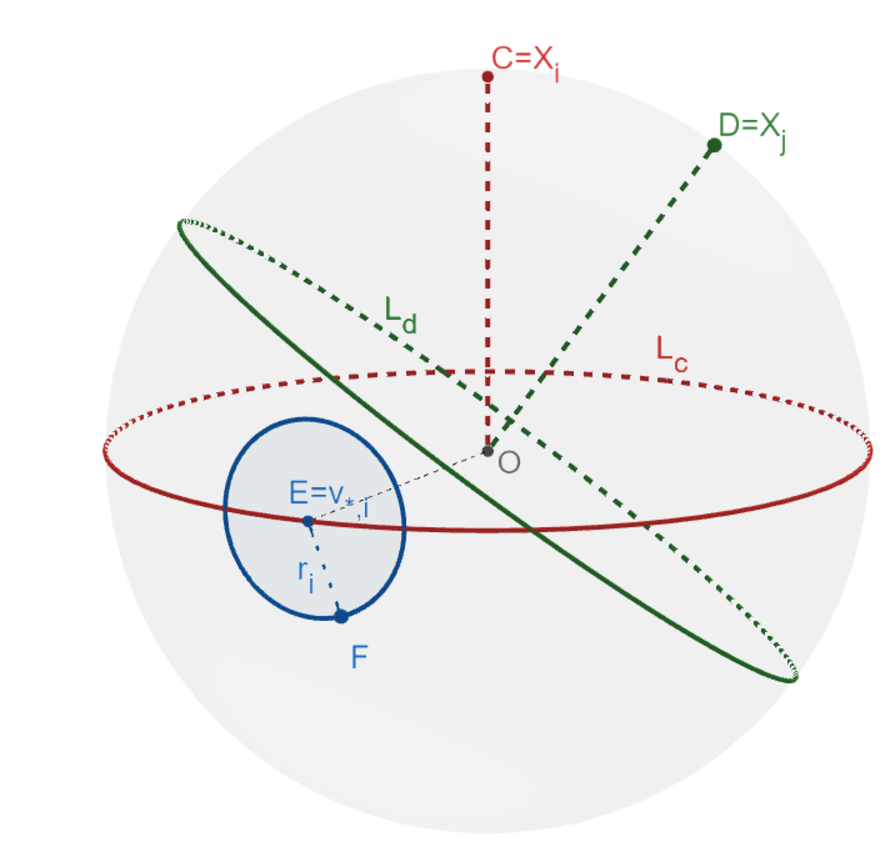
Define a cap on a unit hyper-sphere 𝒮d−1\mathcal{S}^{d-1} as the intersection of 𝒮d−1\mathcal{S}^{d-1} with an open ball in ℝd\mathds{R}^{d} centered at 𝒗∗\bm{v}_{*} with radius rr, i.e.,

ℬ𝒗∗r:={𝒗∈𝒮d−1|‖𝒗−𝒗∗‖2<r}.\displaystyle\mathcal{B}_{\bm{v}_{*}}^{r}\mathrel{\mathop{:}}=\left\{\bm{v}\in\mathcal{S}^{d-1}\ |\ \|\bm{v}-\bm{v}_{*}\|_{2}<r\right\}. (21)
Remark 4.

For ease of exposition, we will sometimes neglect the subscript 𝒗∗\bm{v}_{*} of ℬ𝒗∗r\mathcal{B}_{\bm{v}_{*}}^{r} and use ℬr\mathcal{B}^{r} instead, when the quantity that we are estimating only depends on rr but not 𝒗∗\bm{v}_{*}. For example, where we are interested in the area of ℬ𝒗∗r\mathcal{B}_{\bm{v}_{*}}^{r}, it only depends on rr but not 𝒗∗\bm{v}_{*}. Thus, we write λd−1​(ℬr)\lambda_{d-1}(\mathcal{B}^{r}) instead.

For any 𝒙∈ℝd\bm{x}\in\mathds{R}^{d} such that 𝒙T​𝒗∗=0\bm{x}^{T}\bm{v}_{*}=0, define two halves of the cap ℬ𝒗∗r\mathcal{B}_{\bm{v}_{*}}^{r} as

ℬ𝒗∗,+r,𝒙:={𝒗∈ℬ𝒗∗r|𝒙T𝒗>0},ℬ𝒗∗,−r,𝒙:={𝒗∈ℬ𝒗∗r|𝒙T𝒗<0}.\displaystyle\mathcal{B}_{\bm{v}_{*},+}^{r,\bm{x}}\mathrel{\mathop{:}}=\left\{\bm{v}\in\mathcal{B}_{\bm{v}_{*}}^{r}\ |\ \bm{x}^{T}\bm{v}>0\right\},\quad\mathcal{B}_{\bm{v}_{*},-}^{r,\bm{x}}\mathrel{\mathop{:}}=\left\{\bm{v}\in\mathcal{B}_{\bm{v}_{*}}^{r}\ |\ \bm{x}^{T}\bm{v}<0\right\}. (22)

Define the set of directions of the initial weights 𝐕0​[j]\mathbf{V}_{0}[j]’s as

𝒜𝐕0:={𝐕0​[j]‖𝐕0​[j]‖2|j∈{1,2,⋯,p}}.\displaystyle\mathcal{A}_{\mathbf{V}_{0}}\mathrel{\mathop{:}}=\left\{\frac{\mathbf{V}_{0}[j]}{\|\mathbf{V}_{0}[j]\|_{2}}\ \Bigg|\ j\in\{1,2,\cdots,p\}\right\}. (23)

Appendix B GD (gradient descent) Converges to Min ℓ2\ell_{2}-Norm Solutions

We assume that the GD algorithm for minimizing the training MSE is given by

Δ​𝐕k+1GD=Δ​𝐕kGD−γk​∑i=1n(𝐇i​Δ​𝐕kGD−yi)​𝐇iT,\displaystyle\Delta\mathbf{V}^{\text{GD}}_{k+1}=\Delta\mathbf{V}^{\text{GD}}_{k}-\gamma_{k}\sum_{i=1}^{n}(\mathbf{H}_{i}\Delta\mathbf{V}^{\text{GD}}_{k}-y_{i})\mathbf{H}_{i}^{T}, (24)

where Δ​𝐕kGD\Delta\mathbf{V}^{\text{GD}}_{k} denotes the solution in the kk-th GD iteration (Δ​𝐕0GD=𝟎\Delta\mathbf{V}^{\text{GD}}_{0}=\bm{0}), and γk\gamma_{k} denotes the step size of the kk-th iteration.

Lemma 6.

If Δ​𝐕ℓ2\Delta\mathbf{V}^{\ell_{2}} exists and GD in Eq. (24) converges to zero-training loss (i.e., 𝐇​Δ​𝐕∞GD=𝐲\mathbf{H}\Delta\mathbf{V}^{\text{GD}}_{\infty}=\bm{y}), then Δ​𝐕∞GD=Δ​𝐕ℓ2\Delta\mathbf{V}^{\text{GD}}_{\infty}=\Delta\mathbf{V}^{\ell_{2}}.

Proof.

Because Δ​𝐕0GD=𝟎\Delta\mathbf{V}^{\text{GD}}_{0}=\bm{0} and Eq. (24), we know that Δ​𝐕kGD\Delta\mathbf{V}^{\text{GD}}_{k} is in the row space of 𝐇\mathbf{H} for any kk. Thus, we can let Δ​𝐕∞GD=𝐇T​𝒂\Delta\mathbf{V}^{\text{GD}}_{\infty}=\mathbf{H}^{T}\bm{a} where 𝒂∈ℝn\bm{a}\in\mathds{R}^{n}. When GD converges to zero training loss, we have 𝐇​Δ​𝐕∞GD=𝒚\mathbf{H}\Delta\mathbf{V}^{\text{GD}}_{\infty}=\bm{y}. Thus, we have 𝐇𝐇T​𝒂=𝒚\mathbf{H}\mathbf{H}^{T}\bm{a}=\bm{y}, which implies 𝒂=(𝐇𝐇T)−1​𝒚\bm{a}=(\mathbf{H}\mathbf{H}^{T})^{-1}\bm{y}. Therefore, we must have Δ​𝐕∞GD=𝐇T​𝒂=𝐇T​(𝐇𝐇T)−1​𝒚=Δ​𝐕ℓ2\Delta\mathbf{V}^{\text{GD}}_{\infty}=\mathbf{H}^{T}\bm{a}=\mathbf{H}^{T}(\mathbf{H}\mathbf{H}^{T})^{-1}\bm{y}=\Delta\mathbf{V}^{\ell_{2}}. ∎

Appendix C Assumptions and Justifications

Because f^Δ​𝐕,𝐕0​(a​𝒙)=a⋅f^Δ​𝐕,𝐕0​(𝒙)\hat{f}_{\Delta\mathbf{V},\mathbf{V}_{0}}(a\bm{x})=a\cdot\hat{f}_{\Delta\mathbf{V},\mathbf{V}_{0}}(\bm{x}) for any a∈ℝa\in\mathds{R}, we can always do preprocessing to normalize the input 𝒙\bm{x}. For simplicity, we focus on the simplest situation that the randomness for the inputs and the initial weights are uniform. Nonetheless, methods and results of this paper can be readily generalized to other continuous random variable distributions, which we leave for future work. We thus make the following Assumption 1.

Assumption 1.

The input 𝐱\bm{x} are uniformly distributed in 𝒮d−1\mathcal{S}^{d-1}. The initial weights 𝐕0​[j]\mathbf{V}_{0}[j]’s are uniform in all directions. In other words, μ⁡(⋅)\mu(\cdot) and λ~​(⋅)\tilde{\lambda}(\cdot) are both 𝗎𝗇𝗂𝖿⁡(𝒮d−1)\mathsf{unif}(\mathcal{S}^{d-1}).

We study the overparameterized and overfitted setting, so in this paper we always assume p≥n/dp\geq n/d, i.e., the number of parameters p​dpd is larger than or equal to the number of training samples nn. The situation of d=1d=1 is relatively trivial, so we only consider the case d≥2d\geq 2. We then make Assumption 2.

Assumption 2.

p≥n/dp\geq n/d and d≥2d\geq 2.

If the input is a continuous random vector, then for any i≠ji\neq j, we have 𝖯𝗋{𝐗i=𝐗j}=0\prob\{\mathbf{X}_{i}=\mathbf{X}_{j}\}=0 and 𝖯𝗋{𝐗i=−𝐗j}=0\prob\{\mathbf{X}_{i}=-\mathbf{X}_{j}\}=0 (because the probability that a continuous random variable equals to a given value is zero). Thus, 𝖯𝗋{𝐗i∥𝐗j}=0\prob\{\mathbf{X}_{i}\parallel\mathbf{X}_{j}\}=0, and 𝖯𝗋{𝐗i∦𝐗j}=1\prob\{\mathbf{X}_{i}\nparallel\mathbf{X}_{j}\}=1. Similarly, we can show that 𝖯𝗋{𝐕0[k]∦𝐕0[l]}=1\prob\{\mathbf{V}_{0}[k]\nparallel\mathbf{V}_{0}[l]\}=1. We thus make Assumption 3.

Assumption 3.

𝐗i∦𝐗j\mathbf{X}_{i}\nparallel\mathbf{X}_{j} for any i≠ji\neq j, and 𝐕0​[k]∦𝐕0​[l]\mathbf{V}_{0}[k]\nparallel\mathbf{V}_{0}[l] for any k≠lk\neq l.

With these assumptions, the following lemma says that when pp is large enough, with high probability 𝐇\mathbf{H} has full row-rank (and thus Δ​𝐕ℓ2\Delta\mathbf{V}^{\ell_{2}} exists).

Lemma 7.

limp→∞𝖯𝗋𝐕0​{𝗋𝖺𝗇𝗄(𝐇)=n|𝐗}=1\lim_{p\to\infty}\underset{\mathbf{V}_{0}}{\prob}\left\{\rank(\mathbf{H})=n\ |\ \mathbf{X}\right\}=1.

Proof.

See Appendix E. ∎

Appendix D Some Useful Supporting Results

Here we collect some useful lemmas that are needed for proofs in other appendices, many of which are estimations of certain quantities that we will use later.

D.1 Quantities related to the area of a cap on a hyper-sphere

The following lemma is introduced by Li 2011, which gives the area of a cap on a hyper-sphere with respect to the colatitude angle.

Lemma 8.

Let ϕ∈[0,π2]\phi\in[0,\ \frac{\pi}{2}] denote the colatitude angle of the smaller cap on 𝒮d−1\mathcal{S}^{d-1}, then the area (in the measure of λd−1\lambda_{d-1}) of this hyper-spherical cap is

12​λd−1​(𝒮d−1)​Isin2⁡ϕ​(d−12,12).\displaystyle\frac{1}{2}\lambda_{d-1}(\mathcal{S}^{d-1})I_{\sin^{2}\phi}\left(\frac{d-1}{2},\frac{1}{2}\right).

The following lemma is another representation of the area of the cap with respect to the radius rr (recall the definition of ℬr\mathcal{B}^{r} in Eq. (21) and Remark 4).

Lemma 9.

If r≤2r\leq\sqrt{2}, then we have

λd−1​(ℬr)=12​λd−1​(𝒮d−1)​Ir2​(1−r24)​(d−12,12).\displaystyle\lambda_{d-1}(\mathcal{B}^{r})=\frac{1}{2}\lambda_{d-1}(\mathcal{S}^{d-1})I_{r^{2}(1-\frac{r^{2}}{4})}\left(\frac{d-1}{2},\frac{1}{2}\right).
Proof.

Let ϕ\phi denote the colatitude angle. By the law of cosines, we have

cos⁡ϕ=1−r22.\displaystyle\cos\phi=1-\frac{r^{2}}{2}.

Thus, we have

sin2⁡ϕ=1−cos2⁡ϕ=1−(1−r22)2=r2​(1−r24).\displaystyle\sin^{2}\phi=1-\cos^{2}\phi=1-\left(1-\frac{r^{2}}{2}\right)^{2}=r^{2}\left(1-\frac{r^{2}}{4}\right).

By Lemma 8, the result of this lemma thus follows. Notice that we require r≤2r\leq\sqrt{2} to make sure that ϕ∈[0,π2]\phi\in[0,\ \frac{\pi}{2}], which is required by Lemma 8. ∎

The area of a cap can be interpreted as the probability of the event that a uniformly-distributed random vector falls into that cap. We have the following lemma.

Lemma 10.

Suppose that a random vector 𝐛∈𝒮d−1\bm{b}\in\mathcal{S}^{d-1} follows uniform distribution in all directions. Given any 𝐚∈𝒮d−1\bm{a}\in\mathcal{S}^{d-1} and for any c∈(0,1)c\in(0,1), we have

𝖯𝗋𝐛{|𝐚T𝐛|>c}=I1−c2(d−12,12).\displaystyle\prob_{\bm{b}}\left\{|\bm{a}^{T}\bm{b}|>c\right\}=I_{1-c^{2}}\left(\frac{d-1}{2},\frac{1}{2}\right).
Proof.

Notice that {𝒃|𝒂T​𝒃>c}\left\{\bm{b}\ \big|\ \bm{a}^{T}\bm{b}>c\right\} is a hyper-spherical cap. Define its colatitude angle as ϕ\phi. We have cos⁡ϕ=𝒂T​𝒃=c\cos\phi=\bm{a}^{T}\bm{b}=c. Thus, we have sin2⁡ϕ=1−c2\sin^{2}\phi=1-c^{2}. By Lemma 8, we then have

λd−1​({𝒃|𝒂T​𝒃>c})=12​λd−1​(𝒮d−1)​I1−c2​(d−12,12).\displaystyle\lambda_{d-1}\left(\left\{\bm{b}\ \big|\ \bm{a}^{T}\bm{b}>c\right\}\right)=\frac{1}{2}\lambda_{d-1}(\mathcal{S}^{d-1})I_{1-c^{2}}\left(\frac{d-1}{2},\frac{1}{2}\right).

Further, by symmetry, we have

λd−1​({𝒃||𝒂T​𝒃|>c})=2​λd−1​({𝒃|𝒂T​𝒃>c})=λd−1​(𝒮d−1)​I1−c2​(d−12,12).\displaystyle\lambda_{d-1}\left(\left\{\bm{b}\ \big|\ |\bm{a}^{T}\bm{b}|>c\right\}\right)=2\lambda_{d-1}\left(\left\{\bm{b}\ \big|\ \bm{a}^{T}\bm{b}>c\right\}\right)=\lambda_{d-1}(\mathcal{S}^{d-1})I_{1-c^{2}}\left(\frac{d-1}{2},\frac{1}{2}\right).

Because 𝒃\bm{b} follows uniform distribution in all directions, we have

𝖯𝗋𝐛{|𝐚T𝐛|>c}=λd−1​({𝐛||𝐚T​𝐛|>c})λd−1​(𝒮d−1)=I1−c2(d−12,12).\displaystyle\prob_{\bm{b}}\left\{|\bm{a}^{T}\bm{b}|>c\right\}=\frac{\lambda_{d-1}\left(\left\{\bm{b}\ \big|\ |\bm{a}^{T}\bm{b}|>c\right\}\right)}{\lambda_{d-1}(\mathcal{S}^{d-1})}=I_{1-c^{2}}\left(\frac{d-1}{2},\frac{1}{2}\right).

∎

D.2 Estimation of certain norms

In this subsection, we will show ‖𝒉𝐕0,𝒙‖2≤p\|\bm{h}_{\mathbf{V}_{0},\bm{x}}\|_{2}\leq\sqrt{p} in Lemma 11. We also upper bound the norm of the product of two matrices by the product of their norms in Lemma 12. At last, Lemma 13 states that if two vector differ a lot, then the sum of their norm cannot be too small.

Lemma 11.

‖𝒉𝐕0,𝒙‖2≤p\|\bm{h}_{\mathbf{V}_{0},\bm{x}}\|_{2}\leq\sqrt{p} for any 𝐱∈𝒮d−1\bm{x}\in\mathcal{S}^{d-1}.

Proof.

This follows because the input 𝒙\bm{x} is normalized. Specifically, by Eq. (1), we have

‖𝒉𝐕0,𝒙‖2=∑j=1p‖𝟏{𝒙T𝐕0[j]>0}⋅𝒙T‖22≤p.\displaystyle\|\bm{h}_{\mathbf{V}_{0},\bm{x}}\|_{2}=\sqrt{\sum_{j=1}^{p}\left\|\bm{1}_{\{\bm{x}^{T}\mathbf{V}_{0}[j]>0\}}\cdot\bm{x}^{T}\right\|_{2}^{2}}\leq\sqrt{p}. (25)

∎

Lemma 12.

If 𝐂=𝐀𝐁\mathbf{C}=\mathbf{A}\mathbf{B}, then ‖𝐂‖2≤‖𝐀‖2⋅‖𝐁‖2\|\mathbf{C}\|_{2}\leq\|\mathbf{A}\|_{2}\cdot\|\mathbf{B}\|_{2}. Here 𝐀\mathbf{A}, 𝐁\mathbf{B}, and 𝐂\mathbf{C} could be scalars, vectors, or matrices.

Proof.

This lemma directly follows the definition of matrix norm. ∎

Remark 5.

Note that the (ℓ2\ell_{2}) matrix-norm (i.e., spectral norm) of a vector is exactly its ℓ2\ell_{2} vector-norm (i.e., Euclidean norm)77 7 To see this, consider a (row or column) vector 𝒂\bm{a}. The matrix norm of 𝒂\bm{a} is max|x|=1⁡‖𝒂​x‖2​ (when 𝒂 is a column vector),\displaystyle\max_{|x|=1}\|\bm{a}x\|_{2}\text{ (when $\bm{a}$ is a column vector)}, or max‖𝒙‖2=1⁡‖𝒂​𝒙‖2​ (when 𝒂 is a row vector).\displaystyle\max_{\|\bm{x}\|_{2}=1}\|\bm{a}\bm{x}\|_{2}\text{ (when $\bm{a}$ is a row vector)}. In both cases, the value of the matrix-norm equals to ∑ai2\sqrt{\sum a_{i}^{2}}, which is exactly the ℓ2\ell_{2}-norm (Euclidean norm) of 𝒂\bm{a}. . Therefore, when applying Lemma 12, we do not need to worry about whether 𝐀\mathbf{A}, 𝐁\mathbf{B}, and 𝐂\mathbf{C} are matrices or vectors.

Lemma 13.

For any 𝐯1,𝐯2∈ℝd\bm{v}_{1},\bm{v}_{2}\in\mathds{R}^{d}, we have

‖𝒗1‖22+‖𝒗2‖22≥12​‖𝒗1−𝒗2‖22.\displaystyle\|\bm{v}_{1}\|_{2}^{2}+\|\bm{v}_{2}\|_{2}^{2}\geq\frac{1}{2}\|\bm{v}_{1}-\bm{v}_{2}\|_{2}^{2}.
Proof.

It is easy to prove that ∥⋅∥22\|\cdot\|_{2}^{2} is convex. Thus, we have

‖𝒗1‖22+‖𝒗2‖22\displaystyle\|\bm{v}_{1}\|_{2}^{2}+\|\bm{v}_{2}\|_{2}^{2} =‖𝒗1‖22+‖−𝒗2‖22\displaystyle=\|\bm{v}_{1}\|_{2}^{2}+\|-\bm{v}_{2}\|_{2}^{2}
≥2​‖𝒗1−𝒗22‖22​ (apply Jensen’s inequality on the convex function ∥⋅∥22)\displaystyle\geq 2\left\|\frac{\bm{v}_{1}-\bm{v}_{2}}{2}\right\|_{2}^{2}\text{ (apply Jensen's inequality on the convex function $\|\cdot\|_{2}^{2}$)}
=12​‖𝒗1−𝒗2‖22.\displaystyle=\frac{1}{2}\|\bm{v}_{1}-\bm{v}_{2}\|_{2}^{2}.

∎

D.3 Estimates of certain tail probabilities

The following is the (restated) Corollary 5 of Goemans 2015.

Lemma 14.

If the random variable XX follows 𝖡𝗂𝗇𝗈⁡(a,b)\mathsf{Bino}(a,b), then for all 0<δ<10<\delta<1, we have

𝖯𝗋{|X−ab|>δab}≤2e−abδ2/3.\displaystyle\prob\{|X-ab|>\delta ab\}\leq 2e^{-ab\delta^{2}/3}.

The following lemma is the (restated) Theorem 1.8 of Hayes 2005.

Lemma 15 (Azuma–Hoeffding inequality for random vectors).

Let X1,X2,⋯,XkX_{1},X_{2},\cdots,X_{k} be i.i.d. random vectors with zero mean (of the same dimension) in a real Euclidean space such that ‖Xi‖2≤1\|X_{i}\|_{2}\leq 1 for all i=1,2,⋯,ki=1,2,\cdots,k. Then, for every a>0a>0,

𝖯𝗋{‖∑i=1kXi‖2≥a}<2e2exp(−a22​k).\displaystyle\prob\left\{\left\|\sum_{i=1}^{k}X_{i}\right\|_{2}\geq a\right\}<2e^{2}\exp\left(-\frac{a^{2}}{2k}\right).

In the following lemma, we use Azuma–Hoeffding inequality to upper bound the deviation of the empirical mean value of a bounded random vector from its expectation.

Lemma 16.

Let X1,X2,⋯,XkX_{1},X_{2},\cdots,X_{k} be i.i.d. random vectors (of the same dimension) in a real Euclidean space such that ‖Xi‖2≤U\|X_{i}\|_{2}\leq U for all i=1,2,⋯,ki=1,2,\cdots,k. Then, for any q∈[1,∞)q\in[1,\ \infty),

𝖯𝗋{‖(1k∑i=1kXi)−𝖤X1‖2≥k12​q−12}<2e2exp(−kq8​U2).\displaystyle\prob\left\{\left\|\left(\frac{1}{k}\sum_{i=1}^{k}X_{i}\right)-\expectation X_{1}\right\|_{2}\geq k^{\frac{1}{2q}-\frac{1}{2}}\right\}<2e^{2}\exp\left(-\frac{\sqrt[q]{k}}{8U^{2}}\right).
Proof.

Because ‖Xi‖2≤U\|X_{i}\|_{2}\leq U, we have 𝖤‖Xi‖2≤U\expectation\|X_{i}\|_{2}\leq U. By triangle inequality, we have ‖Xi−𝖤Xi‖2≤‖Xi‖2+𝖤‖Xi‖2≤2​U\|X_{i}-\expectation X_{i}\|_{2}\leq\|X_{i}\|_{2}+\expectation\|X_{i}\|_{2}\leq 2U, i.e.,

‖Xi−𝖤Xi2​U‖2≤1.\displaystyle\left\|\frac{X_{i}-\expectation X_{i}}{2U}\right\|_{2}\leq 1. (26)

We also have

𝖤[Xi−𝖤Xi2​U]=𝖤Xi−𝖤Xi2​U=𝟎.\displaystyle\expectation\left[\frac{X_{i}-\expectation X_{i}}{2U}\right]=\frac{\expectation X_{i}-\expectation X_{i}}{2U}=\bm{0}. (27)

We then have

𝖯𝗋{‖(1k∑i=1kXi)−𝖤X1‖2≥k12​q−12}\displaystyle\prob\left\{\left\|\left(\frac{1}{k}\sum_{i=1}^{k}X_{i}\right)-\expectation X_{1}\right\|_{2}\geq k^{\frac{1}{2q}-\frac{1}{2}}\right\}
=\displaystyle= 𝖯𝗋{‖∑i=1k(Xi−𝖤Xi)‖2≥k12​q+12}\displaystyle\prob\left\{\left\|\sum_{i=1}^{k}\left(X_{i}-\expectation X_{i}\right)\right\|_{2}\geq k^{\frac{1}{2q}+\frac{1}{2}}\right\}
=\displaystyle= 𝖯𝗋{‖∑i=1k(Xi−𝖤Xi2​U)‖2≥k12​q+122​U}\displaystyle\prob\left\{\left\|\sum_{i=1}^{k}\left(\frac{X_{i}-\expectation X_{i}}{2U}\right)\right\|_{2}\geq\frac{k^{\frac{1}{2q}+\frac{1}{2}}}{2U}\right\}
<\displaystyle< 2​e2​exp⁡(−kq8​U2)​ (by Eqs. (26)(27) and letting a=k12​q+122​U in Lemma 15).\displaystyle 2e^{2}\exp\left(-\frac{\sqrt[q]{k}}{8U^{2}}\right)\text{ (by Eqs.~\eqref{eq.temp_120308}\eqref{eq.temp_022601} and letting $a=\frac{k^{\frac{1}{2q}+\frac{1}{2}}}{2U}$ in Lemma~\ref{le.hoeffding})}.

∎

D.4 Calculation of certain integrals

The following lemma calculates the ratio between the intersection area of two hyper-hemispheres and the area of the whole hyper-sphere.

Lemma 17.
∫𝒮d−1𝟏{𝒛T​𝒗>0,𝒙T​𝒗>0}​𝑑λ~​(𝒗)=π−arccos⁡(𝒙T​𝒛)2​π.\displaystyle\int_{\mathcal{S}^{d-1}}\bm{1}_{\{\bm{z}^{T}\bm{v}>0,\ \bm{x}^{T}\bm{v}>0\}}d\tilde{\lambda}(\bm{v})=\frac{\pi-\arccos(\bm{x}^{T}\bm{z})}{2\pi}. (28)

(Recall that λ~​(⋅)\tilde{\lambda}(\cdot) denotes the distribution of the normalized version of 𝐕0​[j]\mathbf{V}_{0}[j] on 𝒮d−1\mathcal{S}^{d-1} and is assumed to be uniform in all directions.)

Before we give the proof of Lemma 17, we give its geometric explanation.

Geometric explanation of Eq. (28): Indeed, since λ~\tilde{\lambda} is uniform on 𝒮d−1\mathcal{S}^{d-1}, the integral on the left-hand-side of Eq. (28) represents the probability that a random point falls into the intersection of two hyper-hemispheres that are represented by {𝒗∈𝒮d−1|𝒛T​𝒗>0}\{\bm{v}\in\mathcal{S}^{d-1}\ |\ \bm{z}^{T}\bm{v}>0\} and {𝒗∈𝒮d−1|𝒙T​𝒗>0}\{\bm{v}\in\mathcal{S}^{d-1}\ |\ \bm{x}^{T}\bm{v}>0\}, respectively. We can calculate that probability by

measure of a hyper-spherical lune with angle π−θ⁡(𝒛,𝒙)measure of a unit hyper-sphere=π−arccos⁡(𝒙T​𝒛)2​π,\displaystyle\frac{\text{measure of a hyper-spherical lune with angle $\pi-\theta(\bm{z},\bm{x})$}}{\text{measure of a unit hyper-sphere}}=\frac{\pi-\arccos(\bm{x}^{T}\bm{z})}{2\pi}, (29)

where θ⁡(⋅,⋅)\theta(\cdot,\cdot) denote the angle (in radians) between two vectors, which would lead to Eq. (28).

Refer to caption
Figure 4: The arc CBF⌢\stackrel{{\scriptstyle\frown}}{{\mathrm{CBF}}} is π−θ2​π\frac{\pi-\theta}{2\pi} of the perimeter of the circle O\mathrm{O}.
Refer to caption
Figure 5: The area of the spherical lune ICHF\mathrm{ICHF} is π−θ2​π\frac{\pi-\theta}{2\pi} of the area of the whole sphere.

To help readers understand Eq. (29), we give examples for 2D and 3D in Fig. 4 and Fig. 5, respectively. In the 2D case depicted in Fig. 4, OA→\overrightarrow{\mathrm{OA}} denotes 𝒛\bm{z}, OB→\overrightarrow{\mathrm{OB}} denotes 𝒙\bm{x}. Thus, the arc EAF⌢\stackrel{{\scriptstyle\frown}}{{\mathrm{EAF}}} denotes {𝒗|𝒛T​𝒗>0}\{\bm{v}\ |\ \bm{z}^{T}\bm{v}>0\}, and the arc CBD⌢\stackrel{{\scriptstyle\frown}}{{\mathrm{CBD}}} denotes {𝒗|𝒙T​𝒗>0}\{\bm{v}\ |\ \bm{x}^{T}\bm{v}>0\}. The intersection of EAF⌢\stackrel{{\scriptstyle\frown}}{{\mathrm{EAF}}} and CBD⌢\stackrel{{\scriptstyle\frown}}{{\mathrm{CBD}}}, i.e., the arc CBF⌢\stackrel{{\scriptstyle\frown}}{{\mathrm{CBF}}}, represents {𝒗|𝒛T𝒗>0,𝒙T𝒗>0}\{\bm{v}\ |\ \bm{z}^{T}\bm{v}>0,\bm{x}^{T}\bm{v}>0\}. Notice that the angle of CBF⌢\stackrel{{\scriptstyle\frown}}{{\mathrm{CBF}}} equals π−θ\pi-\theta, where θ\theta denotes the angle between 𝒛\bm{z} and 𝒙\bm{x}. Therefore, ratio of the length of CBF⌢\stackrel{{\scriptstyle\frown}}{{\mathrm{CBF}}} to the perimeter of the circle equals to ∠​COF2​π=π−θ2​π\frac{\angle\mathrm{COF}}{2\pi}=\frac{\pi-\theta}{2\pi}. Similarly, in the 3D case depicted in Fig. 5, the spherical lune ICHF\mathrm{ICHF} denotes the intersection of the semi-sphere in the direction of OA→\overrightarrow{\mathrm{OA}} and the semi-sphere in the direction of OB→\overrightarrow{\mathrm{OB}}. We can see that the area of the spherical lune ICHF\mathrm{ICHF} is still proportional to the angle ∠​COF\angle\mathrm{COF}. Thus, we still have the result that the area of the spherical lune ICHF\mathrm{ICHF} is π−θ2​π\frac{\pi-\theta}{2\pi} of the area of the whole sphere. The proof below, on the other hand, applies to arbitrary dimensions.

Proof.

Due to symmetry, we know that the integral of Eq. (28) only depends on the angle between 𝒙\bm{x} and 𝒛\bm{z}. Thus, without loss of generality, we let

𝒙=[𝒙1𝒙2⋯𝒙d]=[0 0⋯ 0 1 0]T,𝒛=[0 0⋯ 0cosθsinθ]T,\displaystyle\bm{x}=[\bm{x}_{1}\ \bm{x}_{2}\ \cdots\ \bm{x}_{d}]=[0\ 0\ \cdots\ 0\ 1\ 0]^{T},\ \bm{z}=[0\ 0\ \cdots\ 0\ \cos\theta\ \sin\theta]^{T},

where

θ=arccos⁡(𝒙T​𝒛)∈[0,π].\displaystyle\theta=\arccos(\bm{x}^{T}\bm{z})\in[0,\ \pi]. (30)

Thus, for any 𝒗=[𝒗1𝒗2⋯𝒗d]T\bm{v}=[\bm{v}_{1}\ \bm{v}_{2}\ \cdots\ \bm{v}_{d}]^{T} that makes 𝒛T​𝒗>0\bm{z}^{T}\bm{v}>0 and 𝒙T​𝒗>0\bm{x}^{T}\bm{v}>0, it only needs to satisfy

[cos⁡θ​sin⁡θ]​[𝒗d−1𝒗d]>0,[1 0]​[𝒗d−1𝒗d]>0.\displaystyle[\cos\theta\ \sin\theta]\begin{bmatrix}\bm{v}_{d-1}\\ \bm{v}_{d}\end{bmatrix}>0,\quad[1\ 0]\begin{bmatrix}\bm{v}_{d-1}\\ \bm{v}_{d}\end{bmatrix}>0. (31)

We compute the spherical coordinates 𝝋𝒙=[φ1𝒙φ2𝒙⋯φd−1𝒙]T\bm{\varphi}_{\bm{x}}=[\varphi_{1}^{\bm{x}}\ \varphi_{2}^{\bm{x}}\ \cdots\ \varphi_{d-1}^{\bm{x}}]^{T} where φ1𝒙,⋯,φd−2𝒙∈[0,π]\varphi_{1}^{\bm{x}},\cdots,\varphi_{d-2}^{\bm{x}}\in[0,\pi] and φd−1𝒙∈[0,2​π)\varphi_{d-1}^{\bm{x}}\in[0,2\pi) with the convention that

𝒙1=cos⁡(φ1𝒙),\displaystyle\bm{x}_{1}=\cos(\varphi_{1}^{\bm{x}}),
𝒙2=sin⁡(φ1𝒙)​cos⁡(φ2𝒙),\displaystyle\bm{x}_{2}=\sin(\varphi_{1}^{\bm{x}})\cos(\varphi_{2}^{\bm{x}}),
𝒙3=sin⁡(φ1𝒙)​sin⁡(φ2𝒙)​cos⁡(φ3𝒙),\displaystyle\bm{x}_{3}=\sin(\varphi_{1}^{\bm{x}})\sin(\varphi_{2}^{\bm{x}})\cos(\varphi_{3}^{\bm{x}}),
𝒙d−1=sin(φ1𝒙)sin(φ2𝒙)⋯sin(φd−2𝒙)cos(φd−1𝒙),\displaystyle\bm{x}_{d-1}=\sin(\varphi_{1}^{\bm{x}})\sin(\varphi_{2}^{\bm{x}})\cdots\sin(\varphi_{d-2}^{\bm{x}})\cos(\varphi_{d-1}^{\bm{x}}),
𝒙d=sin(φ1𝒙)sin(φ2𝒙)⋯sin(φd−2𝒙)sin(φd−1𝒙).\displaystyle\bm{x}_{d}=\sin(\varphi_{1}^{\bm{x}})\sin(\varphi_{2}^{\bm{x}})\cdots\sin(\varphi_{d-2}^{\bm{x}})\sin(\varphi_{d-1}^{\bm{x}}).

Thus, we have 𝝋𝒙=[π/2π/2⋯π/2 0]T\bm{\varphi}_{\bm{x}}=[\pi/2\ \pi/2\ \cdots\ \pi/2\ 0]^{T}. Similarly, the spherical coordinates for 𝒛\bm{z} is 𝝋𝒛=[π/2π/2⋯π/2θ]T\bm{\varphi}_{\bm{z}}=[\pi/2\ \pi/2\ \cdots\pi/2\ \theta]^{T}. Let the spherical coordinates for 𝒗\bm{v} be 𝝋𝒗=[φ1𝒗φ2𝒗⋯φd−1𝒗]T\bm{\varphi}_{\bm{v}}=[\varphi_{1}^{\bm{v}}\ \varphi_{2}^{\bm{v}}\ \cdots\ \varphi_{d-1}^{\bm{v}}]^{T}. Thus, Eq. (31) is equivalent to

sin(φ1𝒗)sin(φ2𝒗)⋯sin(φd−2𝒗)(cosθcos(φd−1𝒗)+sinθsin(φd−1𝒗))>0,\displaystyle\sin(\varphi_{1}^{\bm{v}})\sin(\varphi_{2}^{\bm{v}})\cdots\sin(\varphi_{d-2}^{\bm{v}})\left(\cos\theta\cos(\varphi_{d-1}^{\bm{v}})+\sin\theta\sin(\varphi_{d-1}^{\bm{v}})\right)>0, (32)
sin(φ1𝒗)sin(φ2𝒗)⋯sin(φd−2𝒗)cos(φd−1𝒗)>0.\displaystyle\sin(\varphi_{1}^{\bm{v}})\sin(\varphi_{2}^{\bm{v}})\cdots\sin(\varphi_{d-2}^{\bm{v}})\cos(\varphi_{d-1}^{\bm{v}})>0. (33)

Because φ1𝒗,⋯,φd−2𝒗∈[0,π]\varphi_{1}^{\bm{v}},\cdots,\varphi_{d-2}^{\bm{v}}\in[0,\pi] (by the convention of spherical coordinates), we have

sin(φ1𝒗)sin(φ2𝒗)⋯sin(φd−2𝒗)≥0.\displaystyle\sin(\varphi_{1}^{\bm{v}})\sin(\varphi_{2}^{\bm{v}})\cdots\sin(\varphi_{d-2}^{\bm{v}})\geq 0.

Thus, for Eq. (32) and Eq. (33), we have

cos⁡(θ−φd−1𝒗)>0,cos⁡(φd−1𝒗)>0,\displaystyle\cos(\theta-\varphi_{d-1}^{\bm{v}})>0,\quad\cos(\varphi_{d-1}^{\bm{v}})>0,

i.e., φd−1𝒗∈(−π/2,π/2)∩(θ−π/2,θ+π/2)(mod2​π)\varphi_{d-1}^{\bm{v}}\in(-\pi/2,\ \pi/2)\cap(\theta-\pi/2,\ \theta+\pi/2)\pmod{2\pi}. We have

∫𝒮d−1𝟏{𝒛T​𝒗>0,𝒙T​𝒗>0}​𝑑λ~​(𝒗)\displaystyle\int_{\mathcal{S}^{d-1}}\bm{1}_{\{\bm{z}^{T}\bm{v}>0,\ \bm{x}^{T}\bm{v}>0\}}d\tilde{\lambda}(\bm{v})
=\displaystyle= ∫(−π2,π2)∩(θ−π2,θ+π2)∫0π⋯∫0πsind−2(φ1)sind−3(φ2)⋯sin(φd−2)dφ1dφ2⋯dφd−1∫02​π∫0π⋯∫0πsind−2(φ1)sind−3(φ2)⋯sin(φd−2)dφ1dφ2⋯dφd−1\displaystyle\frac{\int_{(-\frac{\pi}{2},\ \frac{\pi}{2})\cap(\theta-\frac{\pi}{2},\ \theta+\frac{\pi}{2})}\int_{0}^{\pi}\cdots\int_{0}^{\pi}\sin^{d-2}(\varphi_{1})\sin^{d-3}(\varphi_{2})\cdots\sin(\varphi_{d-2})\ d\varphi_{1}\ d\varphi_{2}\cdots d\varphi_{d-1}}{\int_{0}^{2\pi}\int_{0}^{\pi}\cdots\int_{0}^{\pi}\sin^{d-2}(\varphi_{1})\sin^{d-3}(\varphi_{2})\cdots\sin(\varphi_{d-2})\ d\varphi_{1}\ d\varphi_{2}\cdots d\varphi_{d-1}}
=\displaystyle= ∫(−π2,π2)∩(θ−π2,θ+π2)A⋅d​φd−1∫02​πA⋅d​φd−1\displaystyle\frac{\int_{(-\frac{\pi}{2},\ \frac{\pi}{2})\cap(\theta-\frac{\pi}{2},\ \theta+\frac{\pi}{2})}A\cdot d\varphi_{d-1}}{\int_{0}^{2\pi}A\cdot d\varphi_{d-1}}
(by defining A:=∫0π⋯∫0πsind−2(φ1)sind−3(φ2)⋯sin(φd−2)dφ1dφ2A\mathrel{\mathop{:}}=\int_{0}^{\pi}\cdots\int_{0}^{\pi}\sin^{d-2}(\varphi_{1})\sin^{d-3}(\varphi_{2})\cdots\sin(\varphi_{d-2})\ d\varphi_{1}\ d\varphi_{2})
=\displaystyle= length of the interval ​(−π2,π2)∩(θ−π2,θ+π2)2​π\displaystyle\frac{\text{length of the interval }(-\frac{\pi}{2},\ \frac{\pi}{2})\cap(\theta-\frac{\pi}{2},\ \theta+\frac{\pi}{2})}{2\pi}
=\displaystyle= π−θ2​π​ (because θ∈[0,π] by Eq. (30))\displaystyle\frac{\pi-\theta}{2\pi}\text{ (because $\theta\in[0,\pi]$ by Eq.~\eqref{eq.temp_020901})}
=\displaystyle= π−arccos⁡(𝒙T​𝒛)2​π​ (by Eq. (30)).\displaystyle\frac{\pi-\arccos(\bm{x}^{T}\bm{z})}{2\pi}\text{ (by Eq.~\eqref{eq.temp_020901})}.

The result of this lemma thus follows. ∎

D.5 Limits of |𝒞𝒛,𝒙𝐕0|/p{|\mathcal{C}_{\bm{z},\bm{x}}^{\mathbf{V}_{0}}|}/{p} when p→∞p\to\infty

We introduce some notions given by Wainwright 2015.

Glivenko-Cantelli class. Let ℱ\mathscr{F} be a class of integrable real-valued functions with domain 𝒳\mathcal{X}, and let X1k={X1,⋯,Xk}X_{1}^{k}=\{X_{1},\cdots,X_{k}\} be a collection of i.i.d. samples from some distribution ℙ\mathbb{P} over 𝒳\mathcal{X}. Consider the random variable

‖ℙk−ℙ‖ℱ:=supf~∈ℱ|1k​∑i=1kf~​(Xk)−𝖤[f~]|,\displaystyle\|\mathbb{P}_{k}-\mathbb{P}\|_{\mathscr{F}}\mathrel{\mathop{:}}=\sup_{\tilde{f}\in\mathscr{F}}\left|\frac{1}{k}\sum_{i=1}^{k}\tilde{f}(X_{k})-\expectation[\tilde{f}]\right|,

which measures the maximum deviation (over the class ℱ\mathscr{F}) between the sample average 1k​∑i=1kf~​(Xi)\frac{1}{k}\sum_{i=1}^{k}\tilde{f}(X_{i}) and the population average 𝖤[f~]=𝖤[f~​(X)]\expectation[\tilde{f}]=\expectation[\tilde{f}(X)]. We say that ℱ\mathscr{F} is a Glivenko-Cantelli class for ℙ\mathbb{P} if ‖ℙk−ℙ‖ℱ\|\mathbb{P}_{k}-\mathbb{P}\|_{\mathscr{F}} converges to zero in probability as k→∞k\to\infty.

Polynomial discrimination. A class ℱ\mathscr{F} of functions with domain 𝒳\mathcal{X} has polynomial discrimination of order ν≥1\nu\geq 1 if for each positive integer kk and collection X1k={X1,⋯,Xk}X_{1}^{k}=\{X_{1},\cdots,X_{k}\} of kk points in 𝒳\mathcal{X}, the set ℱ⁡(X1k)\mathscr{F}(X_{1}^{k}) has cardinality upper bounded by

card​(ℱ⁡(X1k))≤(k+1)ν.\displaystyle\text{card}(\mathscr{F}(X_{1}^{k}))\leq(k+1)^{\nu}.

The following lemma is shown in Page 108 of Wainwright 2015.

Lemma 18.

Any bounded function class with polynomial discrimination is Glivenko-Cantelli.

For our case, we care about the following value.

||𝒞𝒛,𝒙𝐕0|p−π−arccos⁡(𝒙T​𝒛)2​π|=|1p​∑j=1p𝟏{𝒙T​𝐕0​[j]>0,𝒛T​𝐕0​[j]>0}−𝖤𝐯∼λ~​(⋅)[𝟏{𝐱T​𝐯>0,𝐳T​𝐯>0}]|​ (by Lemma 17).\displaystyle\left|\frac{|\mathcal{C}_{\bm{z},\bm{x}}^{\mathbf{V}_{0}}|}{p}-\frac{\pi-\arccos(\bm{x}^{T}\bm{z})}{2\pi}\right|=\left|\frac{1}{p}\sum_{j=1}^{p}\bm{1}_{\{\bm{x}^{T}\mathbf{V}_{0}[j]>0,\bm{z}^{T}\mathbf{V}_{0}[j]>0\}}-\expectation_{\bm{v}\sim\tilde{\lambda}(\cdot)}[\bm{1}_{\{\bm{x}^{T}\bm{v}>0,\bm{z}^{T}\bm{v}>0\}}]\right|\text{ (by Lemma~\ref{le.spherePortion})}.

In the language of Glivenko-Cantelli class, the function class ℱ∗\mathscr{F}_{*} consists of functions 𝟏{𝒙T​𝒗>0,𝒛T​𝒗>0}\bm{1}_{\{\bm{x}^{T}\bm{v}>0,\bm{z}^{T}\bm{v}>0\}} that map 𝒗∈𝒮d−1\bm{v}\in\mathcal{S}^{d-1} to 00 or 11, where every 𝒙∈𝒮d−1\bm{x}\in\mathcal{S}^{d-1} and 𝒛∈𝒮d−1\bm{z}\in\mathcal{S}^{d-1} corresponds to a distinct function in ℱ∗\mathscr{F}_{*}. According to Lemma 18, we need to calculate the order of the polynomial discrimination for this ℱ∗\mathscr{F}_{*}. Towards this end, we need the following lemma, which can be derived from the quantity Qn,NQ_{n,N} in Wendel 1962 (which is the quantity Qd,kQ_{d,k} in the following lemma).

Lemma 19.

Given 𝐯1,𝐯2,⋯,𝐯k∈𝒮d−1\bm{v}_{1},\bm{v}_{2},\cdots,\bm{v}_{k}\in\mathcal{S}^{d-1}, the number of different values (i.e., the cardinality) of the set {(𝟏{𝐱T𝐯1>0},𝟏{𝐱T𝐯2>0},⋯,𝟏{𝐱T𝐯k>0})|𝐱∈𝒮d−1}\left\{\left(\bm{1}_{\{\bm{x}^{T}\bm{v}_{1}>0\}},\bm{1}_{\{\bm{x}^{T}\bm{v}_{2}>0\}},\cdots,\bm{1}_{\{\bm{x}^{T}\bm{v}_{k}>0\}}\right)\ \big|\ \bm{x}\in\mathcal{S}^{d-1}\right\} is at most Qd,kQ_{d,k}, where

Qd,k:={2​∑i=0d−1(k−1i), if ​k>d,2k, if ​k≤d.\displaystyle Q_{d,k}\mathrel{\mathop{:}}=\begin{cases}2\sum_{i=0}^{d-1}\binom{k-1}{i},&\text{ if }k>d,\\ 2^{k},&\text{ if }k\leq d.\end{cases}

Intuitively, Lemma 19 states the number of different regions that kk hyper-planes through the origin (i.e., the kernel of the inner product with each 𝒗i\bm{v}_{i}) can cut 𝒮d−1\mathcal{S}^{d-1} into, because all 𝒙\bm{x} in one region corresponds to the same value of the tuple (𝟏{𝒙T𝒗1>0},𝟏{𝒙T𝒗2>0},⋯,𝟏{𝒙T𝒗k>0})\left(\bm{1}_{\{\bm{x}^{T}\bm{v}_{1}>0\}},\bm{1}_{\{\bm{x}^{T}\bm{v}_{2}>0\}},\cdots,\bm{1}_{\{\bm{x}^{T}\bm{v}_{k}>0\}}\right). For example, in the 2D case (i.e., d=2d=2), kk diameters of a circle can at most cut the whole circle into 2​k2k (which equals to Q2,kQ_{2,k}) parts. Notice that if some 𝒗i\bm{v}_{i}’s are parallel (thus some diameters are overlapped), then the total number of different parts can only be smaller. That is why Lemma 19 states that the cardinality is “at most” Qd,kQ_{d,k}.

The following lemma shows that the cardinality in Lemma 19 is polynomial in kk.

Lemma 20.

Recall the definition Qd,kQ_{d,k} in Lemma 19. For any integer k≥1k\geq 1 and d≥2d\geq 2, we must have Qd,k≤(k+1)d+1Q_{d,k}\leq(k+1)^{d+1}.

Proof.

When k>dk>d, because (k−1i)≤(k−1)d−1\binom{k-1}{i}\leq(k-1)^{d-1} when i≤d−1i\leq d-1, we have Qd,k=2​∑i=0d−1(k−1i)≤2​d​(k+1)d−1≤(k+1)d+1Q_{d,k}=2\sum\limits_{i=0}^{d-1}\binom{k-1}{i}\leq 2d(k+1)^{d-1}\leq(k+1)^{d+1} (the last step uses k≥1k\geq 1 and k>dk>d). When k≤dk\leq d, because k≥1k\geq 1, we have Qd,k=2k≤(k+1)k≤(k+1)dQ_{d,k}=2^{k}\leq(k+1)^{k}\leq(k+1)^{d}. In summary, for any integer k≥1k\geq 1 and d≥2d\geq 2, the result Qd,k≤(k+1)d+1Q_{d,k}\leq(k+1)^{d+1} always holds. ∎

We can now calculate the order of the polynomial discrimination for the function class ℱ∗\mathscr{F}_{*}. Because

card({(𝟏{𝒙T​𝒗1>0,𝒛T​𝒗1>0},𝟏{𝒙T​𝒗2>0,𝒛T​𝒗2>0},⋯,𝟏{𝒙T​𝒗k>0,𝒛T​𝒗k​0})|𝒙∈𝒮d−1,𝒛∈𝒮d−1})\displaystyle\text{card}\left(\left\{\left(\bm{1}_{\{\bm{x}^{T}\bm{v}_{1}>0,\bm{z}^{T}\bm{v}_{1}>0\}},\bm{1}_{\{\bm{x}^{T}\bm{v}_{2}>0,\bm{z}^{T}\bm{v}_{2}>0\}},\cdots,\bm{1}_{\{\bm{x}^{T}\bm{v}_{k}>0,\bm{z}^{T}\bm{v}_{k}0\}}\right)\ \big|\ \bm{x}\in\mathcal{S}^{d-1},\bm{z}\in\mathcal{S}^{d-1}\right\}\right)
≤\displaystyle\leq card({(𝟏{𝒙T𝒗1>0},𝟏{𝒙T𝒗2>0},⋯,𝟏{𝒙T𝒗k>0})|𝒙∈𝒮d−1})\displaystyle\text{card}\left(\left\{\left(\bm{1}_{\{\bm{x}^{T}\bm{v}_{1}>0\}},\bm{1}_{\{\bm{x}^{T}\bm{v}_{2}>0\}},\cdots,\bm{1}_{\{\bm{x}^{T}\bm{v}_{k}>0\}}\right)\ \big|\ \bm{x}\in\mathcal{S}^{d-1}\right\}\right)
⋅card({(𝟏{𝒛T𝒗1>0},𝟏{𝒛T𝒗2>0},⋯,𝟏{𝒛T𝒗k>0})|𝒛∈𝒮d−1}),\displaystyle\cdot\text{card}\left(\left\{\left(\bm{1}_{\{\bm{z}^{T}\bm{v}_{1}>0\}},\bm{1}_{\{\bm{z}^{T}\bm{v}_{2}>0\}},\cdots,\bm{1}_{\{\bm{z}^{T}\bm{v}_{k}>0\}}\right)\ \big|\ \bm{z}\in\mathcal{S}^{d-1}\right\}\right),

by Lemma 19 and Lemma 20, we know that

card​(ℱ∗​(X1k))≤(Qd,k)2≤(k+1)2​(d+1).\displaystyle\text{card}(\mathscr{F}_{*}(X_{1}^{k}))\leq\left(Q_{d,k}\right)^{2}\leq(k+1)^{2(d+1)}.

(Here X1kX_{1}^{k} means {𝐕0​[1],⋯,𝐕0​[k]}\{\mathbf{V}_{0}[1],\cdots,\mathbf{V}_{0}[k]\}.)

Thus, ℱ∗\mathscr{F}_{*} has polynomial discrimination with order at most 2​(d+1)2(d+1). Notice that all functions in ℱ∗\mathscr{F}_{*} is bounded because their outputs can only be 00 or 11. Therefore, by Lemma 18 (i.e., any bounded function class with polynomial discrimination is Glivenko-Cantelli), we know that ℱ∗\mathscr{F}_{*} is Glivenko-Cantelli. In other words, we have shown the following lemma.

Lemma 21.
sup𝒙,𝒛∈𝒮d−1||𝒞𝒛,𝒙𝐕0|p−π−arccos⁡(𝒙T​𝒛)2​π|→P0, as ​p→∞.\displaystyle\sup_{\bm{x},\bm{z}\in\mathcal{S}^{d-1}}\left|\frac{|\mathcal{C}_{\bm{z},\bm{x}}^{\mathbf{V}_{0}}|}{p}-\frac{\pi-\arccos(\bm{x}^{T}\bm{z})}{2\pi}\right|\stackrel{{\scriptstyle\text{P}}}{{\rightarrow}}0,\text{ as }p\to\infty. (34)

Appendix E Proof of Lemma 7 (𝐇\mathbf{H} has full row-rank with high probability as p→∞p\to\infty)

In this section, we prove Lemma 7, i.e., the matrix 𝐇\mathbf{H} has full row-rank with high probability when p→∞p\to\infty. We first introduce two useful lemmas as follows.

The following lemma states that, given 𝐗\mathbf{X} (that satisfies Assumption 3) and k∈{1,2,⋯,n}k\in\{1,2,\cdots,n\}, there always exists a vector 𝒗∈𝒮d−1\bm{v}\in\mathcal{S}^{d-1} that is only orthogonal to one training input 𝐗k\mathbf{X}_{k} but not orthogonal to other training inputs 𝐗i\mathbf{X}_{i} for all i≠ki\neq k. An intuitive explanation is that, because no training inputs are parallel (as stated in Assumption 3), the total set of vectors that are orthogonal to at least two training inputs is too small. That gives us many options to pick such a vector 𝒗\bm{v} that is only orthogonal to one input but not others.

Lemma 22.

For all k∈{1,2,⋯,n}k\in\{1,2,\cdots,n\} we have

𝒯k:={𝒗∈𝒮d−1|𝒗T𝐗k=0,𝒗T𝐗i≠0,for all i∈{1,2,⋯,n}∖{k}}≠∅.\displaystyle\mathcal{T}_{k}\mathrel{\mathop{:}}=\left\{\bm{v}\in\mathcal{S}^{d-1}\ |\ \bm{v}^{T}\mathbf{X}_{k}=0,\bm{v}^{T}\mathbf{X}_{i}\neq 0,\text{for all }i\in\{1,2,\cdots,n\}\setminus\{k\}\right\}\neq\varnothing.
Proof.

We have

𝒯k\displaystyle\mathcal{T}_{k} =𝒮d−1∩ker⁡(𝐗k)∖(⋃i∈{1,2,⋯,n}∖{k}ker⁡(𝐗i))\displaystyle=\mathcal{S}^{d-1}\cap\ker(\mathbf{X}_{k})\setminus\left(\bigcup_{i\in\{1,2,\cdots,n\}\setminus\{k\}}\ker(\mathbf{X}_{i})\right)
=𝒮d−1∩ker⁡(𝐗k)∖(⋃i∈{1,2,⋯,n}∖{k}(𝒮d−1∩ker⁡(𝐗k)∩ker⁡(𝐗i))).\displaystyle=\mathcal{S}^{d-1}\cap\ker(\mathbf{X}_{k})\setminus\left(\bigcup_{i\in\{1,2,\cdots,n\}\setminus\{k\}}\left(\mathcal{S}^{d-1}\cap\ker(\mathbf{X}_{k})\cap\ker(\mathbf{X}_{i})\right)\right).

Because

dim(𝒮d−1∩ker⁡(𝐗k))=d−2,\displaystyle\dim(\mathcal{S}^{d-1}\cap\ker(\mathbf{X}_{k}))=d-2,
dim(𝒮d−1∩ker⁡(𝐗k)∩ker⁡(𝐗i))=d−3​ for all ​i∈{1,2,⋯,n}∖{k}​ (because 𝐗i∦𝐗k),\displaystyle\dim(\mathcal{S}^{d-1}\cap\ker(\mathbf{X}_{k})\cap\ker(\mathbf{X}_{i}))=d-3\text{ for all }i\in\{1,2,\cdots,n\}\setminus\{k\}\text{ (because $\mathbf{X}_{i}\nparallel\mathbf{X}_{k}$)}, (35)

we have

λd−2​(𝒮d−1∩ker⁡(𝐗k))=λd−2​(𝒮d−2)>0,\displaystyle\lambda_{d-2}(\mathcal{S}^{d-1}\cap\ker(\mathbf{X}_{k}))=\lambda_{d-2}(\mathcal{S}^{d-2})>0,
λd−2​(𝒮d−1∩ker⁡(𝐗k)∩ker⁡(𝐗i))=0​ for all ​i∈{1,2,⋯,n}∖{k}.\displaystyle\lambda_{d-2}\left(\mathcal{S}^{d-1}\cap\ker(\mathbf{X}_{k})\cap\ker(\mathbf{X}_{i})\right)=0\text{ for all }i\in\{1,2,\cdots,n\}\setminus\{k\}. (36)

(When d=2d=2, the set in Eq. (35) is not defined. Nonetheless, Eq. (36) still holds when d=2d=2.) Thus, we have

λd−2​(𝒯k)\displaystyle\lambda_{d-2}(\mathcal{T}_{k}) =λd−2​(𝒮d−1∩ker⁡(𝐗k))−λd−2​(⋃i∈{1,2,⋯,n}∖{k}(𝒮d−1∩ker⁡(𝐗k)∩ker⁡(𝐗i)))\displaystyle=\lambda_{d-2}\left(\mathcal{S}^{d-1}\cap\ker(\mathbf{X}_{k})\right)-\lambda_{d-2}\left(\bigcup_{i\in\{1,2,\cdots,n\}\setminus\{k\}}\left(\mathcal{S}^{d-1}\cap\ker(\mathbf{X}_{k})\cap\ker(\mathbf{X}_{i})\right)\right)
≥λd−2​(𝒮d−1∩ker⁡(𝐗k))−∑i∈{1,2,⋯,n}∖{k}λd−2​(𝒮d−1∩ker⁡(𝐗k)∩ker⁡(𝐗i))\displaystyle\geq\lambda_{d-2}\left(\mathcal{S}^{d-1}\cap\ker(\mathbf{X}_{k})\right)-\sum_{i\in\{1,2,\cdots,n\}\setminus\{k\}}\lambda_{d-2}\left(\mathcal{S}^{d-1}\cap\ker(\mathbf{X}_{k})\cap\ker(\mathbf{X}_{i})\right)
=λd−2​(𝒮d−2)\displaystyle=\lambda_{d-2}(\mathcal{S}^{d-2})
>0.\displaystyle>0.

Therefore, 𝒯k≠∅\mathcal{T}_{k}\neq\varnothing. ∎

Refer to caption
Figure 6: Geometric interpretation of ℬ𝒗∗,i,+ri,𝐗i\mathcal{B}_{\bm{v}_{*,i},+}^{r_{i},\mathbf{X}_{i}} and ℬ𝒗∗,i,−ri,𝐗i\mathcal{B}_{\bm{v}_{*,i},-}^{r_{i},\mathbf{X}_{i}} on a sphere (i.e., 𝒮2\mathcal{S}^{2}).

The following lemma plays an important role in answering whether 𝐇\mathbf{H} has full row-rank. Further, it is also closely related to our estimation on the min⁡𝖾𝗂𝗀⁡(𝐇𝐇T)\min\mathsf{eig}(\mathbf{H}\mathbf{H}^{T}) later in Appendix F.

Lemma 23.

Consider any i∈{1,2,⋯,n}i\in\{1,2,\cdots,n\}. For any 𝐯∗,i∈𝒮d−1\bm{v}_{*,i}\in\mathcal{S}^{d-1} satisfying 𝐯∗,iT​𝐗i=0\bm{v}_{*,i}^{T}\mathbf{X}_{i}=0, we define

ri:=minj∈{1,2,⋯,n}∖{i}⁡|𝒗∗,iT​𝐗j|.\displaystyle r_{i}\mathrel{\mathop{:}}=\min_{j\in\{1,2,\cdots,n\}\setminus\{i\}}\left|\bm{v}_{*,i}^{T}\mathbf{X}_{j}\right|. (37)

If there exist k,l∈{1,⋯,p}k,l\in\{1,\cdots,p\} such that

𝐕0​[k]‖𝐕0​[k]‖2∈ℬ𝒗∗,i,+ri,𝐗i,𝐕0​[l]‖𝐕0​[l]‖2∈ℬ𝒗∗,i,−ri,𝐗i,\displaystyle\frac{\mathbf{V}_{0}[k]}{\|\mathbf{V}_{0}[k]\|_{2}}\in\mathcal{B}_{\bm{v}_{*,i},+}^{r_{i},\mathbf{X}_{i}},\quad\frac{\mathbf{V}_{0}[l]}{\|\mathbf{V}_{0}[l]\|_{2}}\in\mathcal{B}_{\bm{v}_{*,i},-}^{r_{i},\mathbf{X}_{i}}, (38)

then we must have

𝐇j​[k]=𝐇j​[l],for all ​j∈{1,2,⋯,n}∖{i},\displaystyle\mathbf{H}_{j}[k]=\mathbf{H}_{j}[l],\ \text{for all }j\in\{1,2,\cdots,n\}\setminus\{i\}, (39)
𝐇i​[k]=𝐗iT,\displaystyle\mathbf{H}_{i}[k]=\mathbf{X}_{i}^{T}, (40)
𝐇i​[l]=𝟎.\displaystyle\mathbf{H}_{i}[l]=\bm{0}. (41)

(Notice that Eq. (38) implies ri>0r_{i}>0.)

Remark 6.

We first give an intuitive geometric interpretation of Lemma 23. In Fig. 6, the sphere centered at O\mathrm{O} denotes 𝒮d−1\mathcal{S}^{d-1}, the vector OC→\overrightarrow{\mathrm{OC}} denotes 𝐗i\mathbf{X}_{i}, the vector OD→\overrightarrow{\mathrm{OD}} denotes one of other 𝐗j\mathbf{X}_{j}’s, the vector OE→\overrightarrow{\mathrm{OE}} denotes 𝒗∗,i\bm{v}_{*,i}, which is perpendicular to 𝐗i\mathbf{X}_{i} (i.e., 𝐗iT​𝒗∗,i=0\mathbf{X}_{i}^{T}\bm{v}_{*,i}=0). The upper half of the cap E\mathrm{E} denotes ℬ𝒗∗,i,+ri,𝐗i\mathcal{B}_{\bm{v}_{*,i},+}^{r_{i},\mathbf{X}_{i}}, the lower half of the cap E\mathrm{E} denotes ℬ𝒗∗,i,−ri,𝐗i\mathcal{B}_{\bm{v}_{*,i},-}^{r_{i},\mathbf{X}_{i}}. The great circle Lc\mathrm{L_{c}} cuts the sphere into two semi-spheres. The semi-sphere in the direction of OC→\overrightarrow{\mathrm{OC}} corresponds to all vectors 𝒗\bm{v} on the sphere that have positive inner product with 𝐗i\mathbf{X}_{i} (i.e., 𝒗∗,iT​𝐗i>0\bm{v}_{*,i}^{T}\mathbf{X}_{i}>0), and the semi-sphere in the opposite direction of OC→\overrightarrow{\mathrm{OC}} corresponds to all vectors 𝒗\bm{v} on the sphere that have negative inner product with 𝐗i\mathbf{X}_{i} (i.e., 𝒗T​𝐗i<0\bm{v}^{T}\mathbf{X}_{i}<0). The great circle Ld\mathrm{L_{d}} is similar to the great circle Lc\mathrm{L_{c}}, but is perpendicular to the direction OD→\overrightarrow{\mathrm{OD}} (i.e., 𝐗j\mathbf{X}_{j}). By choosing the radius of the cap E\mathrm{E} in Eq. (37), we can ensure that all great circles that are perpendicular to other 𝐗j\mathbf{X}_{j}’s do not pass the cap E\mathrm{E}. In other words, for the two semi-spheres cut by the great circle perpendicular to 𝐗j\mathbf{X}_{j}, j≠ij\neq i, the cap E\mathrm{E} must be contained in one of them. Therefore, vectors on the upper half of the cap E\mathrm{E} and the vectors on the lower half of the cap E\mathrm{E} must have the same sign when calculating the inner product with all 𝐗j\mathbf{X}_{j}’s, for all j≠ij\neq i.

Now, let us consider the meaning of Eq. (38) in this geometric setup depicted in Fig. 6. The expression 𝐕0​[k]‖𝐕0​[k]‖2∈ℬ𝒗∗,i,+ri,𝐗i\frac{\mathbf{V}_{0}[k]}{\|\mathbf{V}_{0}[k]\|_{2}}\in\mathcal{B}_{\bm{v}_{*,i},+}^{r_{i},\mathbf{X}_{i}} means that the direction of 𝐕0​[k]\mathbf{V}_{0}[k] is in the upper half of the cap E\mathrm{E}. By the definition of 𝐇i=𝒉𝐕0,𝐗i\mathbf{H}_{i}=\bm{h}_{\mathbf{V}_{0},\mathbf{X}_{i}} in Eq. (1), we must then have 𝐇i​[k]=𝐗iT\mathbf{H}_{i}[k]=\mathbf{X}_{i}^{T}. Similarly, the expression 𝐕0​[l]‖𝐕0​[l]‖2∈ℬ𝒗∗,i,−ri,𝐗i\frac{\mathbf{V}_{0}[l]}{\|\mathbf{V}_{0}[l]\|_{2}}\in\mathcal{B}_{\bm{v}_{*,i},-}^{r_{i},\mathbf{X}_{i}} means that the direction of 𝐕0​[l]\mathbf{V}_{0}[l] is in the lower half of the cap E\mathrm{E}, and thus 𝐇i​[l]=𝟎\mathbf{H}_{i}[l]=\bm{0}. Then, based on the discussions in the previous paragraph, we know that 𝐕0​[k]\mathbf{V}_{0}[k] and 𝐕0​[l]\mathbf{V}_{0}[l] has the same activation pattern under ReLU for all 𝐗j\mathbf{X}_{j}’s that j≠ij\neq i, which implies that 𝐇j​[k]=𝐇j​[l]\mathbf{H}_{j}[k]=\mathbf{H}_{j}[l]. These are precisely the conclusions in Eqs. (39)(40)(41).

Later in Appendix F, Lemma 23 plays an important role in estimating min𝒂∈𝒮n−1⁡‖𝐇T​𝒂‖22\min_{\bm{a}\in\mathcal{S}^{n-1}}\|\mathbf{H}^{T}\bm{a}\|_{2}^{2}. To see this, let aja_{j} denotes the jj-th element of 𝒂\bm{a}. By Eq. (39), we have ∑j∈{1,2,⋯,n}∖{i}((𝐇T​aj)​[k]−(𝐇T​aj)​[l])=𝟎\sum_{j\in\{1,2,\cdots,n\}\setminus\{i\}}((\mathbf{H}^{T}a_{j})[k]-(\mathbf{H}^{T}a_{j})[l])=\bm{0}. By Eq. (40) and Eq. (41), we have (𝐇T​ai)​[k]−(𝐇T​ai)​[l]=𝐗i(\mathbf{H}^{T}a_{i})[k]-(\mathbf{H}^{T}a_{i})[l]=\mathbf{X}_{i}. Combining them together, we have (𝐇T​𝒂)​[k]−(𝐇T​𝒂)​[l]=ai​𝐗i(\mathbf{H}^{T}\bm{a})[k]-(\mathbf{H}^{T}\bm{a})[l]=a_{i}\mathbf{X}_{i}. As long as aia_{i} is not zero, then regardless values of other elements in 𝒂\bm{a}, we always obtain that 𝐇T​𝒂\mathbf{H}^{T}\bm{a} is a non-zero vector. This implies ‖𝐇T​𝒂‖2>0\|\mathbf{H}^{T}\bm{a}\|_{2}>0, which will be useful for estimating min⁡𝖾𝗂𝗀⁡(𝐇𝐇T)/p\min\mathsf{eig}(\mathbf{H}\mathbf{H}^{T})/p in Appendix F.

Proof.

By the definition of rir_{i}, we have

|𝒗∗,iT​𝐗j|−ri≥0​, for all ​j∈{1,2,⋯,n}∖{i}.\displaystyle|\bm{v}_{*,i}^{T}\mathbf{X}_{j}|-r_{i}\geq 0\text{, for all }j\in\{1,2,\cdots,n\}\setminus\{i\}. (42)

For any j∈{1,2,⋯,n}∖{i}j\in\{1,2,\cdots,n\}\setminus\{i\} and any 𝒗∈ℬ𝒗∗,iri\bm{v}\in\mathcal{B}_{\bm{v}_{*,i}}^{r_{i}}, since ‖𝒗−𝒗∗,i‖2<ri\|\bm{v}-\bm{v}_{*,i}\|_{2}<r_{i}, we have

(𝒗T​𝐗j)​(𝒗∗,iT​𝐗j)\displaystyle(\bm{v}^{T}\mathbf{X}_{j})(\bm{v}_{*,i}^{T}\mathbf{X}_{j}) =((𝒗−𝒗∗,i)T​𝐗j+𝒗∗,iT​𝐗j)​(𝒗∗,iT​𝐗j)\displaystyle=\left((\bm{v}-\bm{v}_{*,i})^{T}\mathbf{X}_{j}+\bm{v}_{*,i}^{T}\mathbf{X}_{j}\right)(\bm{v}_{*,i}^{T}\mathbf{X}_{j})
=(𝒗∗,iT​𝐗j)2+(𝒗∗,iT​𝐗j)​((𝒗−𝒗∗,i)T​𝐗j)\displaystyle=(\bm{v}_{*,i}^{T}\mathbf{X}_{j})^{2}+(\bm{v}_{*,i}^{T}\mathbf{X}_{j})\left((\bm{v}-\bm{v}_{*,i})^{T}\mathbf{X}_{j}\right)
≥(𝒗∗,iT​𝐗j)2−|𝒗∗,iT​𝐗j|⋅|(𝒗−𝒗∗,i)T​𝐗j|\displaystyle\geq(\bm{v}_{*,i}^{T}\mathbf{X}_{j})^{2}-\left|\bm{v}_{*,i}^{T}\mathbf{X}_{j}\right|\cdot\left|(\bm{v}-\bm{v}_{*,i})^{T}\mathbf{X}_{j}\right|
≥(𝒗∗,iT​𝐗j)2−|𝒗∗,iT​𝐗j|⋅‖𝒗−𝒗∗,i‖2​‖𝐗j‖2\displaystyle\geq(\bm{v}_{*,i}^{T}\mathbf{X}_{j})^{2}-\left|\bm{v}_{*,i}^{T}\mathbf{X}_{j}\right|\cdot\left\|\bm{v}-\bm{v}_{*,i}\right\|_{2}\left\|\mathbf{X}_{j}\right\|_{2}
>(𝒗∗,iT​𝐗j)2−|𝒗∗,iT​𝐗j|⋅ri​ (by Eq. (21))\displaystyle>(\bm{v}_{*,i}^{T}\mathbf{X}_{j})^{2}-\left|\bm{v}_{*,i}^{T}\mathbf{X}_{j}\right|\cdot r_{i}\text{ (by Eq.~\eqref{eq.temp_100101})}
=|𝒗∗,iT​𝐗j|(|𝒗∗,iT​𝐗j|−ri)\displaystyle=|\bm{v}_{*,i}^{T}\mathbf{X}_{j}|(|\bm{v}_{*,i}^{T}\mathbf{X}_{j}|-r_{i})
≥0​ (by Eq. (42)).\displaystyle\geq 0\text{ (by Eq.~\eqref{eq.temp_093003})}.

Thus, for any 𝒗1∈ℬ𝒗∗,iri,𝒗2∈ℬ𝒗∗,iri,j∈{1,2,⋯,n}∖{i}\bm{v}_{1}\in\mathcal{B}_{\bm{v}_{*,i}}^{r_{i}},\ \bm{v}_{2}\in\mathcal{B}_{\bm{v}_{*,i}}^{r_{i}},\ j\in\{1,2,\cdots,n\}\setminus\{i\}, we have (𝒗1T​𝐗j)​(𝒗∗,iT​𝐗j)>0(\bm{v}_{1}^{T}\mathbf{X}_{j})(\bm{v}_{*,i}^{T}\mathbf{X}_{j})>0 and (𝒗2T​𝐗j)​(𝒗∗,iT​𝐗j)>0(\bm{v}_{2}^{T}\mathbf{X}_{j})(\bm{v}_{*,i}^{T}\mathbf{X}_{j})>0. It implies that

sign​(𝒗1T​𝐗j)=sign​(𝒗∗,iT​𝐗j)=sign​(𝒗2T​𝐗j).\displaystyle\text{sign}(\bm{v}_{1}^{T}\mathbf{X}_{j})=\text{sign}(\bm{v}_{*,i}^{T}\mathbf{X}_{j})=\text{sign}(\bm{v}_{2}^{T}\mathbf{X}_{j}). (43)

By Eq. (38), we know that both 𝐕0​[k]\mathbf{V}_{0}[k] and 𝐕0​[l]\mathbf{V}_{0}[l] are in ℬ𝒗∗,iri\mathcal{B}_{\bm{v}_{*,i}}^{r_{i}}. Applying Eq. (43), we have

sign​(𝐗jT​𝐕0​[k])=sign​(𝐗jT​𝐕0​[l]),for all ​j∈{1,2,⋯,n}∖{i}.\displaystyle\text{sign}(\mathbf{X}_{j}^{T}\mathbf{V}_{0}[k])=\text{sign}(\mathbf{X}_{j}^{T}\mathbf{V}_{0}[l]),\ \text{for all }j\in\{1,2,\cdots,n\}\setminus\{i\}.

Thus, by Eq. (1), we have

𝐇j[k]=𝟏{𝐗jT𝐕0[k]>0}𝐗jT=𝟏{𝐗jT𝐕0[l]>0}𝐗jT=𝐇j[l],for all j∈{1,2,⋯,n}∖{i}.\displaystyle\mathbf{H}_{j}[k]=\bm{1}_{\{\mathbf{X}_{j}^{T}\mathbf{V}_{0}[k]>0\}}\mathbf{X}_{j}^{T}=\bm{1}_{\{\mathbf{X}_{j}^{T}\mathbf{V}_{0}[l]>0\}}\mathbf{X}_{j}^{T}=\mathbf{H}_{j}[l],\ \text{for all }j\in\{1,2,\cdots,n\}\setminus\{i\}.

By Eq. (22), we have

𝐗iT​𝐕0​[k]>0,𝐗iT​𝐕0​[l]<0.\displaystyle\mathbf{X}_{i}^{T}\mathbf{V}_{0}[k]>0,\ \mathbf{X}_{i}^{T}\mathbf{V}_{0}[l]<0.

Thus, by Eq. (1), we have

𝐇i[k]=𝟏{𝐗iT𝐕0[k]>0}𝐗iT=𝐗iT,𝐇i[l]=𝟏{𝐗iT𝐕0[l]>0}𝐗iT=𝟎.\displaystyle\mathbf{H}_{i}[k]=\bm{1}_{\{\mathbf{X}_{i}^{T}\mathbf{V}_{0}[k]>0\}}\mathbf{X}_{i}^{T}=\mathbf{X}_{i}^{T},\quad\mathbf{H}_{i}[l]=\bm{1}_{\{\mathbf{X}_{i}^{T}\mathbf{V}_{0}[l]>0\}}\mathbf{X}_{i}^{T}=\bm{0}.

∎

Now, we are ready to prove Lemma 7.

Proof.

We prove by contradiction. Suppose on the contrary that with some nonzero probability, the design matrix is not full row-rank as p→∞p\to\infty. Note that when the design matrix is not full row-rank, there exists a set of indices ℐ⊆{1,⋯,n}\mathcal{I}\subseteq\{1,\cdots,n\} such that

∑i∈ℐbi​𝐇i=𝟎,bi≠0​ for all ​i∈ℐ.\displaystyle\sum_{i\in\mathcal{I}}b_{i}\mathbf{H}_{i}=\bm{0},\ b_{i}\neq 0\text{ for all }i\in\mathcal{I}. (44)

The proof will be finished by two steps: 1) find an event 𝒥\mathcal{J} that happens almost surely when p→∞p\to\infty; 2) prove this event 𝒥\mathcal{J} contradicts Eq. (44).

Step 1:

Consider each i∈{1,2,⋯,n}i\in\{1,2,\cdots,n\}. By Lemma 22, we know that there exists a 𝒗∗,i∈𝒮d−1\bm{v}_{*,i}\in\mathcal{S}^{d-1} such that

𝒗∗,iT​𝐗i=0,𝒗∗,iT​𝐗j≠0, for all ​j∈{1,2,⋯,n}∖{i}.\displaystyle\bm{v}_{*,i}^{T}\mathbf{X}_{i}=0,\ \bm{v}_{*,i}^{T}\mathbf{X}_{j}\neq 0,\text{ for all }j\in\{1,2,\cdots,n\}\setminus\{i\}. (45)

Define

ri=minj∈{1,2,⋯,n}∖{i}⁡|𝒗∗,iT​𝐗j|>0.\displaystyle r_{i}=\min_{j\in\{1,2,\cdots,n\}\setminus\{i\}}\left|\bm{v}_{*,i}^{T}\mathbf{X}_{j}\right|>0. (46)

For all i=1,2,⋯,ni=1,2,\cdots,n, we define several events as follows.

𝒥i:={𝒜𝐕0∩ℬ𝒗∗,i,+ri,𝐗i≠∅,𝒜𝐕0∩ℬ𝒗∗,i,−ri,𝐗i≠∅},\displaystyle\mathcal{J}_{i}\mathrel{\mathop{:}}=\left\{\mathcal{A}_{\mathbf{V}_{0}}\cap\mathcal{B}_{\bm{v}_{*,i},+}^{r_{i},\mathbf{X}_{i}}\neq\varnothing,\ \mathcal{A}_{\mathbf{V}_{0}}\cap\mathcal{B}_{\bm{v}_{*,i},-}^{r_{i},\mathbf{X}_{i}}\neq\varnothing\right\},
𝒥i,+={𝒜𝐕0∩ℬ𝒗∗,i,+ri,𝐗i≠∅},\displaystyle\mathcal{J}_{i,+}=\left\{\mathcal{A}_{\mathbf{V}_{0}}\cap\mathcal{B}_{\bm{v}_{*,i},+}^{r_{i},\mathbf{X}_{i}}\neq\varnothing\right\},
𝒥i,−={𝒜𝐕0∩ℬ𝒗∗,i,−ri,𝐗i≠∅},\displaystyle\mathcal{J}_{i,-}=\left\{\mathcal{A}_{\mathbf{V}_{0}}\cap\mathcal{B}_{\bm{v}_{*,i},-}^{r_{i},\mathbf{X}_{i}}\neq\varnothing\right\},
𝒥:=⋂i=1n𝒥i.\displaystyle\mathcal{J}\mathrel{\mathop{:}}=\bigcap_{i=1}^{n}\mathcal{J}_{i}.

(Recall the geometric interpretation in Remark 6. The events 𝒥i,+\mathcal{J}_{i,+} and 𝒥i,−\mathcal{J}_{i,-} mean that there exists 𝐕0​[j]/‖𝐕0​[j]‖2\mathbf{V}_{0}[j]/\|\mathbf{V}_{0}[j]\|_{2} in the upper half and the lower half of the cap E\mathrm{E}, respectively. The event 𝒥i=𝒥i,+∩𝒥i,−\mathcal{J}_{i}=\mathcal{J}_{i,+}\cap\mathcal{J}_{i,-} means that there exist 𝐕0​[j]/‖𝐕0​[j]‖2\mathbf{V}_{0}[j]/\|\mathbf{V}_{0}[j]\|_{2} in both halves of the cap E\mathrm{E}. Finally, the event 𝒥\mathcal{J} occurs when 𝒥i\mathcal{J}_{i} occurs for all ii, although the vector 𝐕0​[j]/‖𝐕0​[j]‖2\mathbf{V}_{0}[j]/\|\mathbf{V}_{0}[j]\|_{2} that falls into the two halves may differ across ii. As we will show later, whenever the event 𝒥\mathcal{J} occurs, the matrix 𝐇\mathbf{H} will have the full row-rank, which is why we are interesting in the probability of the event 𝒥\mathcal{J}.)

Those definitions implies that

𝒥ic=𝒥i,+c∪𝒥i,−c​ for all ​i=1,2,⋯,n,\displaystyle\mathcal{J}_{i}^{c}=\mathcal{J}_{i,+}^{c}\cup\mathcal{J}_{i,-}^{c}\text{ for all }i=1,2,\cdots,n, (47)
𝒥c=⋃i=1n𝒥ic.\displaystyle\mathcal{J}^{c}=\bigcup_{i=1}^{n}\mathcal{J}_{i}^{c}. (48)

Thus, we have

𝖯𝗋𝐕0[𝒥]=\displaystyle\prob_{\mathbf{V}_{0}}[\mathcal{J}]= 1−𝖯𝗋𝐕0[𝒥c]\displaystyle 1-\prob_{\mathbf{V}_{0}}[\mathcal{J}^{c}]
≥\displaystyle\geq 1−∑i=1n𝖯𝗋𝐕0[𝒥ic]​ (by Eq. (48) and the union bound).\displaystyle 1-\sum_{i=1}^{n}\prob_{\mathbf{V}_{0}}[\mathcal{J}_{i}^{c}]\text{ (by Eq.~\eqref{eq.temp_112301} and the union bound)}. (49)

For a fixed ii, recall that by Eq. (46), we have ri>0r_{i}>0. Because ℬ𝒗∗,i,+ri,𝐗i\mathcal{B}_{\bm{v}_{*,i},+}^{r_{i},\mathbf{X}_{i}} and ℬ𝒗∗,i,−ri,𝐗i\mathcal{B}_{\bm{v}_{*,i},-}^{r_{i},\mathbf{X}_{i}} are two halves of ℬ𝒗∗,iri\mathcal{B}_{\bm{v}_{*,i}}^{r_{i}}, we have

λd−1​(ℬ𝒗∗,i,+ri,𝐗i)=λd−1​(ℬ𝒗∗,i,−ri,𝐗i)=12​λd−1​(ℬ𝒗∗,iri).\displaystyle\lambda_{d-1}(\mathcal{B}_{\bm{v}_{*,i},+}^{r_{i},\mathbf{X}_{i}})=\lambda_{d-1}(\mathcal{B}_{\bm{v}_{*,i},-}^{r_{i},\mathbf{X}_{i}})=\frac{1}{2}\lambda_{d-1}(\mathcal{B}_{\bm{v}_{*,i}}^{r_{i}}). (50)

Therefore, we have

𝖯𝗋𝐕0[𝒥ic]≤\displaystyle\prob_{\mathbf{V}_{0}}[\mathcal{J}_{i}^{c}]\leq 𝖯𝗋𝐕0[𝒥i,+c]+𝖯𝗋𝐕0[𝒥i,−c]​ (by Eq. (47) and the union bound)\displaystyle\prob_{\mathbf{V}_{0}}[\mathcal{J}_{i,+}^{c}]+\prob_{\mathbf{V}_{0}}[\mathcal{J}_{i,-}^{c}]\text{ (by Eq.~\eqref{eq.temp_112302} and the union bound)}
=\displaystyle= (1−λd−1​(ℬ𝒗∗,i,+ri,𝐗i)λd−1​(𝒮d−1))p+(1−λd−1​(ℬ𝒗∗,i,−ri,𝐗i)λd−1​(𝒮d−1))p\displaystyle\left(1-\frac{\lambda_{d-1}(\mathcal{B}_{\bm{v}_{*,i},+}^{r_{i},\mathbf{X}_{i}})}{\lambda_{d-1}(\mathcal{S}^{d-1})}\right)^{p}+\left(1-\frac{\lambda_{d-1}(\mathcal{B}_{\bm{v}_{*,i},-}^{r_{i},\mathbf{X}_{i}})}{\lambda_{d-1}(\mathcal{S}^{d-1})}\right)^{p}
(all 𝐕0​[i]\mathbf{V}_{0}[i]’s are independent and Assumption 1)
=\displaystyle= 2​(1−λd−1​(ℬ𝒗∗,iri)2​λd−1​(𝒮d−1))p​ (by Eq. (50)).\displaystyle 2\left(1-\frac{\lambda_{d-1}(\mathcal{B}_{\bm{v}_{*,i}}^{r_{i}})}{2\lambda_{d-1}(\mathcal{S}^{d-1})}\right)^{p}\text{ (by Eq.~\eqref{eq.temp_100102})}.

Notice that rir_{i} is determined only by 𝐗\mathbf{X}, and is independent of 𝐕0\mathbf{V}_{0} and pp. Therefore, we have

limp→∞𝖯𝗋𝐕0[𝒥ic]=0.\displaystyle\lim_{p\to\infty}\prob_{\mathbf{V}_{0}}[\mathcal{J}_{i}^{c}]=0. (51)

Plugging Eq. (51) into Eq. (49), we have

limp→∞𝖯𝗋𝐕0[𝒥]=1​ (because n is finite).\displaystyle\lim_{p\to\infty}\prob_{\mathbf{V}_{0}}[\mathcal{J}]=1\text{ (because $n$ is finite)}.

Step 2:

To complete the proof, it remains to show that the event 𝒥\mathcal{J} contradicts Eq. (44). Towards this end, we assume the event 𝒥\mathcal{J} happens. By Eq. (44), we can pick one i∈ℐi\in\mathcal{I}. Further, by the definition of 𝒥\mathcal{J}, there exists rir_{i} such that 𝒜𝐕0∩ℬ𝒗∗,i,+ri,𝐗i≠∅\mathcal{A}_{\mathbf{V}_{0}}\cap\mathcal{B}_{\bm{v}_{*,i},+}^{r_{i},\mathbf{X}_{i}}\neq\varnothing and 𝒜𝐕0∩ℬ𝒗∗,i,−ri,𝐗i≠∅\mathcal{A}_{\mathbf{V}_{0}}\cap\mathcal{B}_{\bm{v}_{*,i},-}^{r_{i},\mathbf{X}_{i}}\neq\varnothing. In other words, there must exist k,l∈{1,⋯,p}k,l\in\{1,\cdots,p\} such that

𝐕0​[k]‖𝐕0​[k]‖2∈ℬ𝒗∗,i,+ri,𝐗i,𝐕0​[l]‖𝐕0​[l]‖2∈ℬ𝒗∗,i,−ri,𝐗i.\displaystyle\frac{\mathbf{V}_{0}[k]}{\|\mathbf{V}_{0}[k]\|_{2}}\in\mathcal{B}_{\bm{v}_{*,i},+}^{r_{i},\mathbf{X}_{i}},\quad\frac{\mathbf{V}_{0}[l]}{\|\mathbf{V}_{0}[l]\|_{2}}\in\mathcal{B}_{\bm{v}_{*,i},-}^{r_{i},\mathbf{X}_{i}}.

By Lemma 23, we have

𝐇j​[k]=𝐇j​[l],for all ​j∈{1,2,⋯,n}∖{i},\displaystyle\mathbf{H}_{j}[k]=\mathbf{H}_{j}[l],\ \text{for all }j\in\{1,2,\cdots,n\}\setminus\{i\}, (52)
𝐇i​[k]=𝐗iT,𝐇i​[l]=𝟎.\displaystyle\mathbf{H}_{i}[k]=\mathbf{X}_{i}^{T},\quad\mathbf{H}_{i}[l]=\bm{0}. (53)

We now show that 𝐇\mathbf{H} restricted to the columns corresponding to kk and ll cannot be linearly dependent. Specifically, we have

∑j∈ℐbj​𝐇j​[k]\displaystyle\sum_{j\in\mathcal{I}}b_{j}\mathbf{H}_{j}[k] =bi​𝐇i​[k]+∑j∈ℐ∖{i}bj​𝐇j​[k]​ (as we have picked i∈ℐ)\displaystyle=b_{i}\mathbf{H}_{i}[k]+\sum_{j\in\mathcal{I}\setminus\{i\}}b_{j}\mathbf{H}_{j}[k]\text{ (as we have picked $i\in\mathcal{I}$)}
=bi​𝐇i​[k]−bj​𝐇i​[l]+∑j∈ℐbj​𝐇j​[l]​ (by Eq. (52))\displaystyle=b_{i}\mathbf{H}_{i}[k]-b_{j}\mathbf{H}_{i}[l]+\sum_{j\in\mathcal{I}}b_{j}\mathbf{H}_{j}[l]\text{ (by Eq.~\eqref{eq.temp_1000106})}
=bi​𝐗iT+∑j∈ℐbj​𝐇j​[l]​ (by Eq. (53))\displaystyle=b_{i}\mathbf{X}_{i}^{T}+\sum_{j\in\mathcal{I}}b_{j}\mathbf{H}_{j}[l]\text{ (by Eq.~\eqref{eq.temp_100107})}
≠∑j∈ℐbj​𝐇j​[l]​ (because bi≠0).\displaystyle\neq\sum_{j\in\mathcal{I}}b_{j}\mathbf{H}_{j}[l]\text{ (because $b_{i}\neq 0$)}.

This contradicts the assumption Eq. (44) that

∑j∈ℐbj​𝐇j​[k]=∑j∈ℐbj​𝐇j​[l]=𝟎.\displaystyle\sum_{j\in\mathcal{I}}b_{j}\mathbf{H}_{j}[k]=\sum_{j\in\mathcal{I}}b_{j}\mathbf{H}_{j}[l]=\bm{0}.

The result thus follows. ∎

Appendix F Proof of Proposition 4 (the upper bound of the variance)

The following lemma shows the relationship between the variance term and min⁡𝖾𝗂𝗀⁡(𝐇𝐇T)/p\min\mathsf{eig}\left(\mathbf{H}\mathbf{H}^{T}\right)/p.

Lemma 24.
|𝒉𝐕0,𝒙​𝐇T​(𝐇𝐇T)−1​ϵ|≤p​‖ϵ‖2min⁡𝖾𝗂𝗀⁡(𝐇𝐇T).\displaystyle|\bm{h}_{\mathbf{V}_{0},\bm{x}}\mathbf{H}^{T}(\mathbf{H}\mathbf{H}^{T})^{-1}\bm{\epsilon}|\leq\frac{\sqrt{p}\|\bm{\epsilon}\|_{2}}{\sqrt{\min\mathsf{eig}(\mathbf{H}\mathbf{H}^{T})}}.
Proof.

We have

‖𝐇T​(𝐇𝐇T)−1​ϵ‖2=(𝐇T​(𝐇𝐇T)−1​ϵ)T​𝐇T​(𝐇𝐇T)−1​ϵ=ϵT​(𝐇𝐇T)−1​ϵ≤‖ϵ‖2min⁡𝖾𝗂𝗀⁡(𝐇𝐇T).\displaystyle\|\mathbf{H}^{T}(\mathbf{H}\mathbf{H}^{T})^{-1}\bm{\epsilon}\|_{2}=\sqrt{(\mathbf{H}^{T}(\mathbf{H}\mathbf{H}^{T})^{-1}\bm{\epsilon})^{T}\mathbf{H}^{T}(\mathbf{H}\mathbf{H}^{T})^{-1}\bm{\epsilon}}=\sqrt{\bm{\epsilon}^{T}(\mathbf{H}\mathbf{H}^{T})^{-1}\bm{\epsilon}}\leq\frac{\|\bm{\epsilon}\|_{2}}{\sqrt{\min\mathsf{eig}(\mathbf{H}\mathbf{H}^{T})}}. (54)

Thus, we have

|𝒉𝐕0,𝒙​𝐇T​(𝐇𝐇T)−1​ϵ|\displaystyle|\bm{h}_{\mathbf{V}_{0},\bm{x}}\mathbf{H}^{T}(\mathbf{H}\mathbf{H}^{T})^{-1}\bm{\epsilon}|
=\displaystyle= ‖𝒉𝐕0,𝒙​𝐇T​(𝐇𝐇T)−1​ϵ‖2​ (ℓ2-norm of a number equals to its absolute value)\displaystyle\|\bm{h}_{\mathbf{V}_{0},\bm{x}}\mathbf{H}^{T}(\mathbf{H}\mathbf{H}^{T})^{-1}\bm{\epsilon}\|_{2}\text{ ($\ell_{2}$-norm of a number equals to its absolute value)}
≤\displaystyle\leq ‖𝒉𝐕0,𝒙‖2⋅‖𝐇T​(𝐇𝐇T)−1​ϵ‖2​ (by Lemma 12)\displaystyle\|\bm{h}_{\mathbf{V}_{0},\bm{x}}\|_{2}\cdot\|\mathbf{H}^{T}(\mathbf{H}\mathbf{H}^{T})^{-1}\bm{\epsilon}\|_{2}\text{ (by Lemma~\ref{le.matrix_norm})}
≤\displaystyle\leq p​‖ϵ‖2min⁡𝖾𝗂𝗀⁡(𝐇𝐇T)​ (by Lemma 11 and Eq. (54)).\displaystyle\frac{\sqrt{p}\|\bm{\epsilon}\|_{2}}{\sqrt{\min\mathsf{eig}(\mathbf{H}\mathbf{H}^{T})}}\text{ (by Lemma~\ref{le.h_p} and Eq.~\eqref{eq.temp_022801})}.

∎

The following lemma shows our estimation on min⁡𝖾𝗂𝗀⁡(𝐇𝐇T)/p\min\mathsf{eig}\left(\mathbf{H}\mathbf{H}^{T}\right)/p.

Lemma 25.

For any n≥2n\geq 2, m∈[1,ln⁡nln⁡π2]m\in\left[1,\ \frac{\ln n}{\ln\frac{\pi}{2}}\right], d≤n4d\leq n^{4}, if p≥6​Jm​(n,d)​ln⁡(4​n1+1m)p\geq 6J_{m}(n,d)\ln\left(4n^{1+\frac{1}{m}}\right), we must have

𝖯𝗋𝐗,𝐕0{min⁡𝖾𝗂𝗀⁡(𝐇𝐇T)p≥1Jm​(n,d)​n}≥1−2nm.\displaystyle\prob_{\mathbf{X},\mathbf{V}_{0}}\Big\{\frac{\min\mathsf{eig}\left(\mathbf{H}\mathbf{H}^{T}\right)}{p}\geq\frac{1}{J_{m}(n,d)n}\Big\}\geq 1-\frac{2}{\sqrt[m]{n}}.

Proposition 4 directly follows from Lemma 25 and Lemma 24. 88 8 We can see that the key part during the proof of Proposition 4 is to estimate min⁡𝖾𝗂𝗀⁡(𝐇𝐇T)/p{\min\mathsf{eig}\left(\mathbf{H}\mathbf{H}^{T}\right)}/{p}. Lemma 25 shows a lower bound of min⁡𝖾𝗂𝗀⁡(𝐇𝐇T)/p{\min\mathsf{eig}\left(\mathbf{H}\mathbf{H}^{T}\right)}/{p} which is almost Ω⁡(n1−2​d)\Omega(n^{1-2d}) when pp is large. However, our estimation of this value may be loose. We will show a upper bound which is O⁡(n−1d−1)O(n^{-\frac{1}{d-1}}) (see Appendix G).

In rest of this section, we will show how to prove Lemma 25. The following lemma shows that, to estimate min⁡𝖾𝗂𝗀⁡(𝐇𝐇T)/p\min\mathsf{eig}\left(\mathbf{H}\mathbf{H}^{T}\right)/p, it is equivalent to estimate min𝒂∈𝒮n−1⁡‖𝐇T​𝒂‖22/p\min_{\bm{a}\in\mathcal{S}^{n-1}}\|\mathbf{H}^{T}\bm{a}\|_{2}^{2}/p.

Lemma 26.
min⁡𝖾𝗂𝗀⁡(𝐇𝐇T)=min𝒂∈𝒮n−1⁡‖𝐇T​𝒂‖22.\displaystyle\min\mathsf{eig}\left(\mathbf{H}\mathbf{H}^{T}\right)=\min_{\bm{a}\in\mathcal{S}^{n-1}}\|\mathbf{H}^{T}\bm{a}\|_{2}^{2}.
Proof.

Do the singular value decomposition (SVD) of 𝐇T\mathbf{H}^{T} as 𝐇T=𝐔​𝚺​𝐖T\mathbf{H}^{T}=\mathbf{U}\mathbf{\Sigma}\mathbf{W}^{T}, where

𝚺∈ℝ(d​p)×n=𝖽𝗂𝖺𝗀⁡(Σ1,Σ2,⋯,Σn).\displaystyle\mathbf{\Sigma}\in\mathds{R}^{(dp)\times n}=\mathsf{diag}(\Sigma_{1},\Sigma_{2},\cdots,\Sigma_{n}).

By properties of singular values, we have

min𝒂∈𝒮n−1⁡‖𝐇T​𝒂‖22=mini∈{1,2,⋯,n}⁡Σi2.\displaystyle\min_{\bm{a}\in\mathcal{S}^{n-1}}\|\mathbf{H}^{T}\bm{a}\|_{2}^{2}=\min_{i\in\{1,2,\cdots,n\}}\Sigma_{i}^{2}.

We also have

𝐇𝐇T\displaystyle\mathbf{H}\mathbf{H}^{T} =𝐖​𝚺T​𝐔T​𝐔​𝚺​𝐖T\displaystyle=\mathbf{W}\mathbf{\Sigma}^{T}\mathbf{U}^{T}\mathbf{U}\mathbf{\Sigma}\mathbf{W}^{T}
=𝐖​𝚺T​𝚺​𝐖T​ (because 𝐔T​𝐔=𝐈)\displaystyle=\mathbf{W}\mathbf{\Sigma}^{T}\mathbf{\Sigma}\mathbf{W}^{T}\text{ (because $\mathbf{U}^{T}\mathbf{U}=\mathbf{I}$)}
=𝐖​𝖽𝗂𝖺𝗀​(Σ12,Σ22,⋯,Σn2)​𝐖T.\displaystyle=\mathbf{W}\mathsf{diag}(\Sigma_{1}^{2},\Sigma_{2}^{2},\cdots,\Sigma_{n}^{2})\mathbf{W}^{T}.

This equation is indeed the eigenvalue decomposition of 𝐇𝐇T\mathbf{H}\mathbf{H}^{T}, which implies that its eigenvalues are Σ12,Σ22,⋯,Σn2\Sigma_{1}^{2},\Sigma_{2}^{2},\cdots,\Sigma_{n}^{2}. Thus, we have

min⁡𝖾𝗂𝗀⁡(𝐇𝐇T)=mini∈{1,2,⋯,n}⁡Σi2=min𝒂∈𝒮n−1⁡‖𝐇T​𝒂‖22.\displaystyle\min\mathsf{eig}\left(\mathbf{H}\mathbf{H}^{T}\right)=\min_{i\in\{1,2,\cdots,n\}}\Sigma_{i}^{2}=\min_{\bm{a}\in\mathcal{S}^{n-1}}\|\mathbf{H}^{T}\bm{a}\|_{2}^{2}.

∎

Therefore, to finish the proof of Proposition 4, it only remains to estimate min𝒂∈𝒮n−1⁡‖𝐇T​𝒂‖22\min_{\bm{a}\in\mathcal{S}^{n-1}}\|\mathbf{H}^{T}\bm{a}\|_{2}^{2}.

By Lemma 7 and its proof in Appendix E, we have already shown that 𝐇T​𝒂\mathbf{H}^{T}\bm{a} is not likely to be zero (i.e. min𝒂∈𝒮n−1⁡‖𝐇T​𝒂‖22>0\min_{\bm{a}\in\mathcal{S}^{n-1}}\|\mathbf{H}^{T}\bm{a}\|_{2}^{2}>0) when p→∞p\to\infty. Here, we basically use the similar method as in Appendix E, but with more precise quantification.

Recall the definitions in Eqs. (21)(22)(23). For any i∈{1,2,⋯,n}i\in\{1,2,\cdots,n\}, we choose one

𝒗∗,i∈𝒮d−1​ independently of 𝐗j, j≠i, such that ​𝒗∗,iT​𝐗i=0.\displaystyle\bm{v}_{*,i}\in\mathcal{S}^{d-1}\text{ independently of $\mathbf{X}_{j}$, $j\neq i$, such that }\bm{v}_{*,i}^{T}\mathbf{X}_{i}=0. (55)

(Note that here, unlike in Eq. (45), we do not require 𝒗∗,iT​𝐗j≠0\bm{v}_{*,i}^{T}\mathbf{X}_{j}\neq 0 for all j≠ij\neq i. This is important as we would like 𝐗j\mathbf{X}_{j} to be independent of 𝒗∗,i\bm{v}_{*,i} for all j≠ij\neq i.) Further, for any 0≤r0≤10\leq r_{0}\leq 1, we define

cr0i:=min⁡{|𝒜𝐕0∩ℬ𝒗∗,i,+r0,𝐗i|,|𝒜𝐕0∩ℬ𝒗∗,i,−r0,𝐗i|}.\displaystyle c_{r_{0}}^{i}\mathrel{\mathop{:}}=\min\left\{|\mathcal{A}_{\mathbf{V}_{0}}\cap\mathcal{B}_{\bm{v}_{*,i},+}^{r_{0},\mathbf{X}_{i}}|,\ |\mathcal{A}_{\mathbf{V}_{0}}\cap\mathcal{B}_{\bm{v}_{*,i},-}^{r_{0},\mathbf{X}_{i}}|\right\}. (56)

Then, we define

ri:=minj∈{1,2,⋯,n}∖{i}⁡|𝒗∗,iT​𝐗j|,\displaystyle r_{i}\mathrel{\mathop{:}}=\min_{j\in\{1,2,\cdots,n\}\setminus\{i\}}\left|\bm{v}_{*,i}^{T}\mathbf{X}_{j}\right|, (57)
r^:=mini∈{1,2,⋯,n}⁡ri.\displaystyle\hat{r}\mathrel{\mathop{:}}=\min_{i\in\{1,2,\cdots,n\}}r_{i}. (58)

(Note that here rir_{i} or r^\hat{r} may be zero. Later we will show that they can be lower bounded with high probability.) Define

D𝐗:=λd−1​(ℬr^)8​n​λd−1​(𝒮d−1).\displaystyle D_{\mathbf{X}}\mathrel{\mathop{:}}=\frac{\lambda_{d-1}(\mathcal{B}^{\hat{r}})}{8n\lambda_{d-1}(\mathcal{S}^{d-1})}. (59)

Similar to Remark 6, these definitions have their geometric interpretation in Fig. 6. The value cr0ic_{r_{0}}^{i} denotes the number of distinct pairs (𝐕0​[k]‖𝐕0​[k]‖2,𝐕0​[l]‖𝐕0​[l]‖2)\left(\frac{\mathbf{V}_{0}[k]}{\|\mathbf{V}_{0}[k]\|_{2}},\frac{\mathbf{V}_{0}[l]}{\|\mathbf{V}_{0}[l]\|_{2}}\right)99 9 Here, “distinct” means that any normalized version of 𝐕0​[j]\mathbf{V}_{0}[j] can appear at most in one pair. such that 𝐕0​[k]‖𝐕0​[k]‖2\frac{\mathbf{V}_{0}[k]}{\|\mathbf{V}_{0}[k]\|_{2}} is in the upper half of the cap E\mathrm{E}, and 𝐕0​[l]‖𝐕0​[l]‖2\frac{\mathbf{V}_{0}[l]}{\|\mathbf{V}_{0}[l]\|_{2}} is in the lower half of the cap E\mathrm{E}. The quantities r0r_{0}, rir_{i}, and r^\hat{r} can all be used as the radius of the cap E\mathrm{E}. The ratio D𝐗D_{\mathbf{X}} is proportional to the area of the cap E\mathrm{E} with radius r^\hat{r} (or equivalently, the probability that the normalized 𝐕0​[j]\mathbf{V}_{0}[j] falls in the cap E\mathrm{E}).

The following lemma gives an estimation on ‖𝐇T​𝒂‖22/p\|\mathbf{H}^{T}\bm{a}\|_{2}^{2}/p when 𝐗\mathbf{X} is given. We put its proof in Appendix F.1.

Lemma 27.

Given 𝐗\mathbf{X}, we have

𝖯𝗋𝐕0{∥𝐇T𝐚∥22≥pD𝐗,for all 𝐚∈𝒮n−1}≥1−4ne−npD𝐗/6.\displaystyle\prob_{\mathbf{V}_{0}}\left\{\|\mathbf{H}^{T}\bm{a}\|_{2}^{2}\geq pD_{\mathbf{X}},\ \text{for all }\bm{a}\in\mathcal{S}^{n-1}\right\}\geq 1-4ne^{-npD_{\mathbf{X}}/6}.

Notice that D𝐗D_{\mathbf{X}} only depends on 𝐗\mathbf{X} and it may even be zero if r^\hat{r} is zero. However, after we introduce the randomness of 𝐗\mathbf{X}, we can show that r^\hat{r} is lower bounded with high probability. We can then obtain the following lemma. We put its proof in Appendix F.2.

Define

Cd:=2​2B⁡(d−12,12),\displaystyle C_{d}\mathrel{\mathop{:}}=\frac{2\sqrt{2}}{B(\frac{d-1}{2},\frac{1}{2})}, (60)
D⁡(n,d,δ):=116​n​Iδ2n4​Cd2​(1−δ24​n4​Cd2)​(d−12,12).\displaystyle D(n,d,\delta)\mathrel{\mathop{:}}=\frac{1}{16n}I_{\frac{\delta^{2}}{n^{4}C_{d}^{2}}\left(1-\frac{\delta^{2}}{4n^{4}C_{d}^{2}}\right)}\left(\frac{d-1}{2},\frac{1}{2}\right). (61)
Lemma 28.

For any δ∈(0,2π]\delta\in\left(0,\frac{2}{\pi}\right], we have

𝖯𝗋𝐗,𝐕0{∥𝐇T𝐚∥22≥pD(n,d,δ),for all 𝐚∈𝒮n−1}≥1−4ne−npD(n,d,δ)/6−δ.\displaystyle\prob_{\mathbf{X},\mathbf{V}_{0}}\left\{\|\mathbf{H}^{T}\bm{a}\|_{2}^{2}\geq pD(n,d,\delta),\ \text{for all }\bm{a}\in\mathcal{S}^{n-1}\right\}\geq 1-4ne^{-npD(n,d,\delta)/6}-\delta.

Notice that Lemma 28 is already very close to Lemma 25, and we put the final steps of the proof of Lemma 25 in Appendix F.3.

F.1 Proof of Lemma 27

Proof.

Define events as follows.

𝒥:={‖𝐇T​𝒂‖22≥p​D𝐗,for all ​𝒂∈𝒮n−1},\displaystyle\mathcal{J}\mathrel{\mathop{:}}=\left\{\|\mathbf{H}^{T}\bm{a}\|_{2}^{2}\geq pD_{\mathbf{X}},\ \text{for all }\bm{a}\in\mathcal{S}^{n-1}\right\},
𝒥i:={there exists 𝒂∈𝒮n−1 that i∈arg​maxj∈{1,2,⋯,n}|aj|,and ∥𝐇T𝐚∥22≤pD𝐗},\displaystyle\mathcal{J}_{i}\mathrel{\mathop{:}}=\left\{\text{there exists }\bm{a}\in\mathcal{S}^{n-1}\text{ that }i\in\argmax_{j\in\{1,2,\cdots,n\}}|a_{j}|,\ \text{and }\|\mathbf{H}^{T}\bm{a}\|_{2}^{2}\leq pD_{\mathbf{X}}\right\},
𝒦i:={crii≤2npD𝐗}, for i=1,2,⋯,n.\displaystyle\mathcal{K}_{i}\mathrel{\mathop{:}}=\left\{c_{r_{i}}^{i}\leq 2npD_{\mathbf{X}}\right\},\text{ for }i=1,2,\cdots,n.

Those definitions directly imply that

𝒥c=⋃i=1n𝒥i.\displaystyle\mathcal{J}^{c}=\bigcup_{i=1}^{n}\mathcal{J}_{i}. (62)

Step 1: prove 𝒥i⊆𝒦i\mathcal{J}_{i}\subseteq\mathcal{K}_{i}

To show 𝒥i⊆𝒦i\mathcal{J}_{i}\subseteq\mathcal{K}_{i}, we only need to prove that 𝒥i\mathcal{J}_{i} implies 𝒦i\mathcal{K}_{i}. To that end, it suffices to show ‖𝐇T​𝒂‖22≥crii2​n\|\mathbf{H}^{T}\bm{a}\|_{2}^{2}\geq\frac{c_{r_{i}}^{i}}{2n} for the vector 𝒂\bm{a} defined in 𝒥i\mathcal{J}_{i}. Because i∈arg​maxj=1n⁡|aj|i\in\argmax_{j=1}^{n}|a_{j}| and ‖𝒂‖2=1\|\bm{a}\|_{2}=1, we have

|ai|≥1n.\displaystyle|a_{i}|\geq\frac{1}{\sqrt{n}}. (63)

By Eq. (56), we can construct criic_{r_{i}}^{i} pairs (kj,lj)(k_{j},l_{j}) for j=1,2,⋯,criij=1,2,\cdots,c_{r_{i}}^{i} (all kjk_{j}’s are different and all ljl_{j}’s are different), such that

𝐕0​[kj]‖𝐕0​[kj]‖2∈ℬ𝒗∗,i,+ri,𝐗i,𝐕0​[lj]‖𝐕0​[lj]‖2∈ℬ𝒗∗,i,−ri,𝐗i.\displaystyle\frac{\mathbf{V}_{0}[k_{j}]}{\|\mathbf{V}_{0}[k_{j}]\|_{2}}\in\mathcal{B}_{\bm{v}_{*,i},+}^{r_{i},\mathbf{X}_{i}},\quad\frac{\mathbf{V}_{0}[l_{j}]}{\|\mathbf{V}_{0}[l_{j}]\|_{2}}\in\mathcal{B}_{\bm{v}_{*,i},-}^{r_{i},\mathbf{X}_{i}}.

Thus, we have

(𝐇T​𝒂)​[kj]−(𝐇T​𝒂)​[lj]=\displaystyle(\mathbf{H}^{T}\bm{a})[k_{j}]-(\mathbf{H}^{T}\bm{a})[l_{j}]= ∑k=1nak​(𝐇k​[kj]−𝐇k​[lj])\displaystyle\sum_{k=1}^{n}a_{k}\left(\mathbf{H}_{k}[k_{j}]-\mathbf{H}_{k}[l_{j}]\right)
=\displaystyle= ai​(𝐇i​[kj]−𝐇i​[lj])+∑k∈{1,2,⋯,n}∖{i}ak​(𝐇k​[kj]−𝐇k​[lj])\displaystyle a_{i}\left(\mathbf{H}_{i}[k_{j}]-\mathbf{H}_{i}[l_{j}]\right)+\sum_{k\in\{1,2,\cdots,n\}\setminus\{i\}}a_{k}\left(\mathbf{H}_{k}[k_{j}]-\mathbf{H}_{k}[l_{j}]\right)
=\displaystyle= ai​𝐗i​ (by Lemma 23).\displaystyle a_{i}\mathbf{X}_{i}\text{ (by Lemma~\ref{le.split_half})}.

We then have

‖(𝐇T​𝒂)​[kj]‖22+‖(𝐇T​𝒂)​[lj]‖22\displaystyle\|(\mathbf{H}^{T}\bm{a})[k_{j}]\|_{2}^{2}+\|(\mathbf{H}^{T}\bm{a})[l_{j}]\|_{2}^{2} ≥12​‖ai​𝐗i‖22​ (by Lemma 13)\displaystyle\geq\frac{1}{2}\|a_{i}\mathbf{X}_{i}\|_{2}^{2}\text{ (by Lemma~\ref{le.l2_diff})}
≥12​n​ (by Eq. (63)).\displaystyle\geq\frac{1}{2n}\text{ (by Eq.~\eqref{eq.temp_100401})}.

Further, we have

‖𝐇T​𝒂‖22\displaystyle\|\mathbf{H}^{T}\bm{a}\|_{2}^{2} =∑j=1p‖(𝐇T​𝒂)​[j]‖22≥∑j=1crii‖(𝐇T​𝒂)​[kj]‖22+‖(𝐇T​𝒂)​[lj]‖22=crii2​n.\displaystyle=\sum_{j=1}^{p}\|(\mathbf{H}^{T}\bm{a})[j]\|_{2}^{2}\geq\sum_{j=1}^{c_{r_{i}}^{i}}\|(\mathbf{H}^{T}\bm{a})[k_{j}]\|_{2}^{2}+\|(\mathbf{H}^{T}\bm{a})[l_{j}]\|_{2}^{2}=\frac{c_{r_{i}}^{i}}{2n}. (64)

Clearly, if the event 𝒥i\mathcal{J}_{i} occurs, then ‖𝐇​𝒂‖22≤p​D𝐗\|\mathbf{H}\bm{a}\|_{2}^{2}\leq pD_{\mathbf{X}}. Combining with Eq. (64), we then have crii≤2​n​p​D𝐗c_{r_{i}}^{i}\leq 2npD_{\mathbf{X}}. In other words, the event 𝒦i\mathcal{K}_{i} must occur. Hence, we have shown that 𝒥i⊆𝒦i\mathcal{J}_{i}\subseteq\mathcal{K}_{i}.

Step 2: estimate the probability of 𝒦i\mathcal{K}_{i}

For all j∈{1,2,⋯,p}j\in\{1,2,\cdots,p\}, because 𝐕0​[j]\mathbf{V}_{0}[j] is uniformly distributed in all directions, for any fixed 0≤r0≤10\leq r_{0}\leq 1, we have

𝖯𝗋𝐕0{𝐕0​[j]‖𝐕0​[j]‖2∈ℬ𝐯∗,i,+r0,𝐗i|i}=λd−1​(ℬ𝐯∗r0)2​λd−1​(𝒮d−1).\displaystyle\prob_{\mathbf{V}_{0}}\left\{\frac{\mathbf{V}_{0}[j]}{\|\mathbf{V}_{0}[j]\|_{2}}\in\mathcal{B}_{\bm{v}_{*,i},+}^{r_{0},\mathbf{X}_{i}}\Bigg|\ i\right\}=\frac{\lambda_{d-1}(\mathcal{B}_{\bm{v}_{*}}^{r_{0}})}{2\lambda_{d-1}(\mathcal{S}^{d-1})}.

Thus, |𝒜𝐕0∩ℬ𝒗∗,i,+r0,𝐗i||\mathcal{A}_{\mathbf{V}_{0}}\cap\mathcal{B}_{\bm{v}_{*,i},+}^{r_{0},\mathbf{X}_{i}}| follows the distribution 𝖡𝗂𝗇𝗈⁡(p,λd−1​(ℬ𝒗∗r0)2​λd−1​(𝒮d−1))\mathsf{Bino}\left(p,\ \frac{\lambda_{d-1}(\mathcal{B}_{\bm{v}_{*}}^{r_{0}})}{2\lambda_{d-1}(\mathcal{S}^{d-1})}\right) given i​ and ​𝐗i\text{ and }\mathbf{X}. By Lemma 14 (with δ=12\delta=\frac{1}{2}), we have

𝖯𝗋𝐕0{|𝒜𝐕0∩ℬ𝐯∗,i,+r0,𝐗i|<p​λd−1​(ℬ𝐯∗r0)4​λd−1​(𝒮d−1)|i}≤2​exp⁡(−p​λd−1​(ℬ𝐯∗r0)48​λd−1​(𝒮d−1)).\displaystyle\prob_{\mathbf{V}_{0}}\left\{|\mathcal{A}_{\mathbf{V}_{0}}\cap\mathcal{B}_{\bm{v}_{*,i},+}^{r_{0},\mathbf{X}_{i}}|<\frac{p\lambda_{d-1}(\mathcal{B}_{\bm{v}_{*}}^{r_{0}})}{4\lambda_{d-1}(\mathcal{S}^{d-1})}\Big|\ i\right\}\leq 2\exp\left(-\frac{p\lambda_{d-1}(\mathcal{B}_{\bm{v}_{*}}^{r_{0}})}{48\lambda_{d-1}(\mathcal{S}^{d-1})}\right). (65)

Similarly, we have

𝖯𝗋𝐕0{|𝒜𝐕0∩ℬ𝐯∗,i,−r0,𝐗i|<p​λd−1​(ℬ𝐯∗r0)4​λd−1​(𝒮d−1)|i}≤2​exp⁡(−p​λd−1​(ℬ𝐯∗r0)48​λd−1​(𝒮d−1)).\displaystyle\prob_{\mathbf{V}_{0}}\left\{|\mathcal{A}_{\mathbf{V}_{0}}\cap\mathcal{B}_{\bm{v}_{*,i},-}^{r_{0},\mathbf{X}_{i}}|<\frac{p\lambda_{d-1}(\mathcal{B}_{\bm{v}_{*}}^{r_{0}})}{4\lambda_{d-1}(\mathcal{S}^{d-1})}\Big|\ i\right\}\leq 2\exp\left(-\frac{p\lambda_{d-1}(\mathcal{B}_{\bm{v}_{*}}^{r_{0}})}{48\lambda_{d-1}(\mathcal{S}^{d-1})}\right). (66)

By plugging Eq. (65) and Eq. (66) into Eq. (56) and applying the union bound, we have

𝖯𝗋𝐕0{cr0i<p​λd−1​(ℬ𝐯∗r0)4​λd−1​(𝒮d−1)|i}≤4​exp⁡(−p​λd−1​(ℬ𝐯∗r0)48​λd−1​(𝒮d−1)).\displaystyle\prob_{\mathbf{V}_{0}}\left\{c_{r_{0}}^{i}<\frac{p\lambda_{d-1}(\mathcal{B}_{\bm{v}_{*}}^{r_{0}})}{4\lambda_{d-1}(\mathcal{S}^{d-1})}\Big|\ i\right\}\leq 4\exp\left(-\frac{p\lambda_{d-1}(\mathcal{B}_{\bm{v}_{*}}^{r_{0}})}{48\lambda_{d-1}(\mathcal{S}^{d-1})}\right).

By letting r0=r^r_{0}=\hat{r} and by Eq. (59), we thus have

𝖯𝗋𝐕0{crii≤2​n​p​D𝐗|i}≤4​exp⁡(−16​npD𝐗),\displaystyle\prob_{\mathbf{V}_{0}}\left\{c_{r_{i}}^{i}\leq 2npD_{\mathbf{X}}\Big|\ i\right\}\leq 4\exp\left(-\frac{1}{6}npD_{\mathbf{X}}\right),

i.e.,

𝖯𝗋𝐕0[𝒦i]≤4exp(−16npD𝐗), for all i=1,2,⋯,n.\displaystyle\prob_{\mathbf{V}_{0}}[\mathcal{K}_{i}]\leq 4\exp\left(-\frac{1}{6}npD_{\mathbf{X}}\right),\text{ for all }i=1,2,\cdots,n. (67)

Step3: estimate the probability of 𝒥\mathcal{J}

We have

𝖯𝗋𝐕0[𝒥c]≤\displaystyle\prob_{\mathbf{V}_{0}}[\mathcal{J}^{c}]\leq ∑i=1n𝖯𝗋𝐕0[𝒥i]​ (by Eq. (62) and the union bound)\displaystyle\sum_{i=1}^{n}\prob_{\mathbf{V}_{0}}[\mathcal{J}_{i}]\text{ (by Eq.~\eqref{eq.temp_112405} and the union bound)}
≤\displaystyle\leq ∑i=1n𝖯𝗋𝐕0[𝒦i]​ (by 𝒥i⊆𝒦i proven in Step 1)\displaystyle\sum_{i=1}^{n}\prob_{\mathbf{V}_{0}}[\mathcal{K}_{i}]\text{ (by $\mathcal{J}_{i}\subseteq\mathcal{K}_{i}$ proven in Step 1)}
≤\displaystyle\leq 4​n​exp⁡(−16​n​p​D𝐗)​ (by Eq. (67)).\displaystyle 4n\exp\left(-\frac{1}{6}npD_{\mathbf{X}}\right)\text{ (by Eq.~\eqref{eq.temp_020301})}.

Thus, we have

𝖯𝗋𝐕0[𝒥]=1−𝖯𝗋𝐕0[𝒥c]≥1−4​n​exp⁡(−16​npD𝐗).\displaystyle\prob_{\mathbf{V}_{0}}[\mathcal{J}]=1-\prob_{\mathbf{V}_{0}}[\mathcal{J}^{c}]\geq 1-4n\exp\left(-\frac{1}{6}npD_{\mathbf{X}}\right).

The result of this lemma thus follows. ∎

F.2 Proof of Lemma 28

Based on Lemma 27, it remains to estimate r^\hat{r}, which will then allow us to bound D𝐗D_{\mathbf{X}}. Towards this end, we need a few lemmas to estimate B⁡(d−12,12)B\left(\frac{d-1}{2},\ \frac{1}{2}\right) and Ix​(d−12,12)I_{x}\left(\frac{d-1}{2},\frac{1}{2}\right).

Lemma 29.

For any x∈ℝx\in\mathds{R}, we must have x+1≤exx+1\leq e^{x}.

Proof.

Consider a function g⁡(x)=ex−x−1g(x)=e^{x}-x-1. It remains to show that g⁡(x)≥0g(x)\geq 0 for all xx. We have g′​(x)=ex−1g^{\prime}(x)=e^{x}-1. In other words, g′​(x)≤0g^{\prime}(x)\leq 0 when x≤0x\leq 0, and g′​(x)≥0g^{\prime}(x)\geq 0 when x≥0x\geq 0. Thus, g⁡(x)g(x) is monotone decreasing when x≤0x\leq 0, and is monotone increasing when x≥0x\geq 0. Hence, we know that g⁡(x)g(x) achieves its minimum value at x=0x=0, i.e., g⁡(x)≥g⁡(0)=0g(x)\geq g(0)=0 for any xx. The conclusion of this lemma thus follows. ∎

Lemma 30.

For any d≥5d\geq 5, we have

(1−1d−3)d−3≥1e2.\displaystyle\left(1-\frac{1}{d-3}\right)^{d-3}\geq\frac{1}{e^{2}}.
Proof.

By letting x=1d−4x=\frac{1}{d-4} in Lemma 29, we have

d−3d−4=1d−4+1≤exp⁡(1d−4),\displaystyle\frac{d-3}{d-4}=\frac{1}{d-4}+1\leq\exp\left(\frac{1}{d-4}\right),

i.e.,

d−4d−3≥exp⁡(−1d−4).\displaystyle\frac{d-4}{d-3}\geq\exp\left(-\frac{1}{d-4}\right). (68)

Thus, we have

(1−1d−3)d−3\displaystyle\left(1-\frac{1}{d-3}\right)^{d-3} =(d−4d−3)d−3\displaystyle=\left(\frac{d-4}{d-3}\right)^{d-3}
≥exp⁡(−d−3d−4)\displaystyle\geq\exp\left(-\frac{d-3}{d-4}\right)
=exp⁡(−1−1d−4)\displaystyle=\exp\left(-1-\frac{1}{d-4}\right)
≥exp⁡(−2)​ (because exp⁡(⋅) is monotone increasing and d≥5).\displaystyle\geq\exp(-2)\text{ (because $\exp(\cdot)$ is monotone increasing and $d\geq 5$)}.

∎

Lemma 31.

For any d≥5d\geq 5, we must have

2e​1d−3≥2e​1d\displaystyle\frac{2}{e}\sqrt{\frac{1}{d-3}}\geq\frac{2}{e}\frac{1}{\sqrt{d}}
Proof.

The result directly follows by d−3≤dd-3\leq d when d≥5d\geq 5. ∎

Lemma 32.
B⁡(d−12,12)∈[2e​1d,π].\displaystyle B\left(\frac{d-1}{2},\ \frac{1}{2}\right)\in\left[\frac{2}{e}\frac{1}{\sqrt{d}},\ \pi\right].

Further, if d≥5d\geq 5, we have

B⁡(d−12,12)∈[2e​1d,4d−3].\displaystyle B\left(\frac{d-1}{2},\ \frac{1}{2}\right)\in\left[\frac{2}{e}\frac{1}{\sqrt{d}},\ \frac{4}{\sqrt{d-3}}\right].
Proof.

When d=2d=2, we have B⁡(d−12,12)=πB\left(\frac{d-1}{2},\ \frac{1}{2}\right)=\pi. When d=3d=3, we have B⁡(d−12,12)=2B\left(\frac{d-1}{2},\ \frac{1}{2}\right)=2. When d=4d=4, we have B⁡(d−12,12)≈1.57B\left(\frac{d-1}{2},\ \frac{1}{2}\right)\approx 1.57. It is easy to verify that the statement of the lemma holds for d=2d=2, 33, and 44. It remains to validate the case of d≥5d\geq 5. We first prove the lower bound. For any m∈(0,1)m\in(0,1), we have

B⁡(d−12,12)=\displaystyle B\left(\frac{d-1}{2},\ \frac{1}{2}\right)= ∫01td−32​(1−t)−12​𝑑t\displaystyle\int_{0}^{1}t^{\frac{d-3}{2}}(1-t)^{-\frac{1}{2}}dt
≥\displaystyle\geq ∫m1td−32​(1−t)−12​𝑑t​ (because td−32​(1−t)−12≥0)\displaystyle\int_{m}^{1}t^{\frac{d-3}{2}}(1-t)^{-\frac{1}{2}}dt\text{ (because $t^{\frac{d-3}{2}}(1-t)^{-\frac{1}{2}}\geq 0$)}
≥\displaystyle\geq md−32​∫m1(1−t)−12​𝑑t\displaystyle m^{\frac{d-3}{2}}\int_{m}^{1}(1-t)^{-\frac{1}{2}}dt
(because td−32t^{\frac{d-3}{2}} is monotone increasing with respect to tt when d≥5d\geq 5)
=\displaystyle= md−32​(−2​1−t|m1)\displaystyle m^{\frac{d-3}{2}}\left(-2\sqrt{1-t}\ \bigg|_{m}^{1}\right)
=\displaystyle= md−32⋅2​1−m.\displaystyle m^{\frac{d-3}{2}}\cdot 2\sqrt{1-m}.

By letting m=1−1d−3m=1-\frac{1}{d-3}, we thus have

B⁡(d−12,12)≥(1−1d−3)d−32⋅2​1d−3.\displaystyle B\left(\frac{d-1}{2},\ \frac{1}{2}\right)\geq\left(1-\frac{1}{d-3}\right)^{\frac{d-3}{2}}\cdot 2\sqrt{\frac{1}{d-3}}.

Then, applying Lemma 30, we have

B⁡(d−12,12)≥2e⋅1d−3.\displaystyle B\left(\frac{d-1}{2},\ \frac{1}{2}\right)\geq\frac{2}{e}\cdot\sqrt{\frac{1}{d-3}}.

Thus, by Lemma 31, we have

B⁡(d−12,12)≥2e​1d.\displaystyle B\left(\frac{d-1}{2},\ \frac{1}{2}\right)\geq\frac{2}{e}\frac{1}{\sqrt{d}}.

Now we prove the upper bound. For any m∈(0,1)m\in(0,1), we have

B⁡(d−12,12)=\displaystyle B\left(\frac{d-1}{2},\ \frac{1}{2}\right)= ∫01td−32​(1−t)−12​𝑑t\displaystyle\int_{0}^{1}t^{\frac{d-3}{2}}(1-t)^{-\frac{1}{2}}dt
=\displaystyle= ∫0mtd−32​(1−t)−12​𝑑t+∫m1td−32​(1−t)−12​𝑑t\displaystyle\int_{0}^{m}t^{\frac{d-3}{2}}(1-t)^{-\frac{1}{2}}dt+\int_{m}^{1}t^{\frac{d-3}{2}}(1-t)^{-\frac{1}{2}}dt
≤\displaystyle\leq ∫0mtd−32​(1−m)−12​𝑑t+∫m1(1−t)−12​𝑑t\displaystyle\int_{0}^{m}t^{\frac{d-3}{2}}(1-m)^{-\frac{1}{2}}dt+\int_{m}^{1}(1-t)^{-\frac{1}{2}}dt
=\displaystyle= 2d−1​md−12​(1−m)−12+2​1−m\displaystyle\frac{2}{d-1}m^{\frac{d-1}{2}}(1-m)^{-\frac{1}{2}}+2\sqrt{1-m}
≤\displaystyle\leq 2d−1​(1−m)−12+2​1−m​ (because m<1 and d≥5).\displaystyle\frac{2}{d-1}(1-m)^{-\frac{1}{2}}+2\sqrt{1-m}\text{ (because $m<1$ and $d\geq 5$)}.

By letting m=1−1d−3m=1-\frac{1}{d-3}, we thus have

B⁡(d−12,12)≤\displaystyle B\left(\frac{d-1}{2},\ \frac{1}{2}\right)\leq 2​d−3d−1+2d−3\displaystyle\frac{2\sqrt{d-3}}{d-1}+\frac{2}{\sqrt{d-3}}
≤\displaystyle\leq 4d−3.\displaystyle\frac{4}{\sqrt{d-3}}.

Notice that 45−3=2​2<π\frac{4}{\sqrt{5-3}}=2\sqrt{2}<\pi. The result of this lemma thus follows.

∎

Lemma 33.

Recall CdC_{d} is defined in Eq. (60). If d≤n4d\leq n^{4} and δ≤1\delta\leq 1, then

(1−δ24​n4​Cd2)d−12≥12.\displaystyle\left(1-\frac{\delta^{2}}{4n^{4}C_{d}^{2}}\right)^{\frac{d-1}{2}}\geq\frac{1}{2}.
Proof.

We have

(1−δ24​n4​Cd2)d−12≥\displaystyle\left(1-\frac{\delta^{2}}{4n^{4}C_{d}^{2}}\right)^{\frac{d-1}{2}}\geq (1−δ24​n4​Cd2)d−1\displaystyle\left(1-\frac{\delta^{2}}{4n^{4}C_{d}^{2}}\right)^{d-1}
≥\displaystyle\geq 1−(d−1)​δ24​n4​Cd2​ (by Bernoulli’s inequality (1+x)a≥1+a​x)\displaystyle 1-\frac{(d-1)\delta^{2}}{4n^{4}C_{d}^{2}}\text{ (by Bernoulli's inequality $(1+x)^{a}\geq 1+ax$)}
=\displaystyle= 1−(d−1)​(B⁡(d−12,12))24​n4⋅8​ (by δ≤1 and Eq. (60))\displaystyle 1-\frac{(d-1)\left(B\left(\frac{d-1}{2},\ \frac{1}{2}\right)\right)^{2}}{4n^{4}\cdot 8}\text{ (by $\delta\leq 1$ and Eq.~\eqref{eq.def_Cd})}
≥\displaystyle\geq 1−(d−1)​π232​n4​ (by Lemma 32)\displaystyle 1-\frac{(d-1)\pi^{2}}{32n^{4}}\text{ (by Lemma~\ref{le.bound_B})}
≥\displaystyle\geq 1−dn4⋅π232\displaystyle 1-\frac{d}{n^{4}}\cdot\frac{\pi^{2}}{32}
≥\displaystyle\geq 12​ (because n4≥d and π≤4).\displaystyle\frac{1}{2}\text{ (because $n^{4}\geq d$ and $\pi\leq 4$)}.

∎

Lemma 34.

For any δ∈(0,2π]\delta\in\left(0,\ \frac{2}{\pi}\right], we must have δn2​Cd≤12\frac{\delta}{n^{2}C_{d}}\leq\frac{1}{\sqrt{2}}.

Proof.

Because Eq. (60), δ≤2π\delta\leq\frac{2}{\pi}, and n≥1n\geq 1, this lemma directly follows by Lemma 32. ∎

Lemma 35.

For any x∈[0, 1]x\in[0,\ 1], we must have

Ix​(d−12,12)≥Cd2​(d−1)​xd−12,\displaystyle I_{x}\left(\frac{d-1}{2},\frac{1}{2}\right)\geq\frac{C_{d}}{\sqrt{2}(d-1)}x^{\frac{d-1}{2}},

and

limx→0Ix​(d−12,12)xd−12=Cd2​(d−1).\displaystyle\lim_{x\to 0}\frac{I_{x}\left(\frac{d-1}{2},\frac{1}{2}\right)}{x^{\frac{d-1}{2}}}=\frac{C_{d}}{\sqrt{2}(d-1)}.
Proof.

we have

Ix​(d−12,12)=\displaystyle I_{x}\left(\frac{d-1}{2},\frac{1}{2}\right)= ∫0xtd−32​(1−t)−12​𝑑tB⁡(d−12,12)\displaystyle\frac{\int_{0}^{x}t^{\frac{d-3}{2}}(1-t)^{-\frac{1}{2}}dt}{B\left(\frac{d-1}{2},\frac{1}{2}\right)}
=\displaystyle= Cd2​2​∫0xtd−32​(1−t)−12​𝑑t​ (by Eq. (60))\displaystyle\frac{C_{d}}{2\sqrt{2}}\int_{0}^{x}t^{\frac{d-3}{2}}(1-t)^{-\frac{1}{2}}dt\text{ (by Eq.~\eqref{eq.def_Cd})}
∈\displaystyle\in [Cd2​2​∫0xtd−32​𝑑t,Cd2​2​1−x​∫0xtd−32​𝑑t]\displaystyle\left[\frac{C_{d}}{2\sqrt{2}}\int_{0}^{x}t^{\frac{d-3}{2}}dt,\ \frac{C_{d}}{2\sqrt{2}\sqrt{1-x}}\int_{0}^{x}t^{\frac{d-3}{2}}dt\right]
(because (1−t)−1/2∈[1,11−x](1-t)^{-1/2}\in\left[1,\frac{1}{\sqrt{1-x}}\right])
∈\displaystyle\in [Cd2​(d−1)​xd−12,Cd2​(d−1)​1−x​xd−12].\displaystyle\left[\frac{C_{d}}{\sqrt{2}(d-1)}x^{\frac{d-1}{2}},\ \frac{C_{d}}{\sqrt{2}(d-1)\sqrt{1-x}}x^{\frac{d-1}{2}}\right].

Thus, we have

Ix​(d−12,12)xd−12∈[Cd2​(d−1),Cd2​(d−1)​1−x],\displaystyle\frac{I_{x}\left(\frac{d-1}{2},\frac{1}{2}\right)}{x^{\frac{d-1}{2}}}\in\left[\frac{C_{d}}{\sqrt{2}(d-1)},\ \frac{C_{d}}{\sqrt{2}(d-1)\sqrt{1-x}}\right],

which implies

limx→0Ix​(d−12,12)xd−12=Cd2​(d−1).\displaystyle\lim_{x\to 0}\frac{I_{x}\left(\frac{d-1}{2},\frac{1}{2}\right)}{x^{\frac{d-1}{2}}}=\frac{C_{d}}{\sqrt{2}(d-1)}.

∎

Lemma 36.

For any x∈[12, 1)x\in\left[\frac{1}{2},\ 1\right) and for any d∈{2,3,⋯}d\in\{2,3,\cdots\}, we have

Ix​(d−12,12)≥1−2​2​(1−x)B⁡(d−12,12).\displaystyle I_{x}\left(\frac{d-1}{2},\frac{1}{2}\right)\geq 1-\frac{2\sqrt{2(1-x)}}{B\left(\frac{d-1}{2},\frac{1}{2}\right)}.

We also have

lim(1−x)→0+1−Ix​(d−12,12)1−x=2B⁡(d−12,12).\displaystyle\lim_{(1-x)\to 0^{+}}\frac{1-I_{x}\left(\frac{d-1}{2},\frac{1}{2}\right)}{\sqrt{1-x}}=\frac{2}{B\left(\frac{d-1}{2},\frac{1}{2}\right)}.
Proof.

By the definition of regularized incomplete beta function in Eq. (20), we have

Ix​(d−12,12)=∫0xtd−12−1​(1−t)−12​𝑑tB⁡(d−12,12)=1−∫x1td−32​(1−t)−12​𝑑tB⁡(d−12,12).\displaystyle I_{x}\left(\frac{d-1}{2},\frac{1}{2}\right)=\frac{\int_{0}^{x}t^{\frac{d-1}{2}-1}(1-t)^{-\frac{1}{2}}dt}{B\left(\frac{d-1}{2},\frac{1}{2}\right)}=1-\frac{\int_{x}^{1}t^{\frac{d-3}{2}}(1-t)^{-\frac{1}{2}}dt}{B\left(\frac{d-1}{2},\frac{1}{2}\right)}.

Thus, it remains to show that

∫x1td−32​(1−t)−12​𝑑t≤2​2​(1−x), and\displaystyle\int_{x}^{1}t^{\frac{d-3}{2}}(1-t)^{-\frac{1}{2}}dt\leq 2\sqrt{2(1-x)},\text{ and} (69)
lim(1−x)→0+∫x1td−32​(1−t)−12​𝑑t1−x=2.\displaystyle\lim_{(1-x)\to 0^{+}}\frac{\int_{x}^{1}t^{\frac{d-3}{2}}(1-t)^{-\frac{1}{2}}dt}{\sqrt{1-x}}=2. (70)

First, we prove Eq. (69). Case 1: d=2d=2. We have

∫x1td−32​(1−t)−12​𝑑t\displaystyle\int_{x}^{1}t^{\frac{d-3}{2}}(1-t)^{-\frac{1}{2}}dt
=\displaystyle= ∫x1t−12​(1−t)−12​𝑑t\displaystyle\int_{x}^{1}t^{-\frac{1}{2}}(1-t)^{-\frac{1}{2}}dt
≤\displaystyle\leq 1x​∫x1(1−t)−12​𝑑t​ (because t−12 is monotone decreasing in [x, 1])\displaystyle\frac{1}{\sqrt{x}}\int_{x}^{1}(1-t)^{-\frac{1}{2}}dt\text{ (because $t^{-\frac{1}{2}}$ is monotone decreasing in $[x,\ 1]$)}
=\displaystyle= 2​1−xx\displaystyle 2\sqrt{\frac{1-x}{x}}
≤\displaystyle\leq 2​2​(1−x)​ (because x≥12).\displaystyle 2\sqrt{2(1-x)}\text{ (because $x\geq\frac{1}{2}$)}.

Case 2: d≥3d\geq 3. Then td−32t^{\frac{d-3}{2}} is monotone increasing in [x, 1][x,\ 1]. Thus, we have

∫x1td−32​(1−t)−12​𝑑t≤∫x1(1−t)−12​𝑑t=2​1−x≤2​2​(1−x).\displaystyle\int_{x}^{1}t^{\frac{d-3}{2}}(1-t)^{-\frac{1}{2}}dt\leq\int_{x}^{1}(1-t)^{-\frac{1}{2}}dt=2\sqrt{1-x}\leq 2\sqrt{2(1-x)}.

To conclude, for all d∈{2,3,⋯}d\in\{2,3,\cdots\}, Eq. (69) holds.

Second, we prove Eq. (70). We have

∫x1td−32​(1−t)−12​𝑑t1−x∈\displaystyle\frac{\int_{x}^{1}t^{\frac{d-3}{2}}(1-t)^{-\frac{1}{2}}dt}{\sqrt{1-x}}\in [min⁡{1,xd−32}​∫x1(1−t)−12​𝑑t1−x,max⁡{1,xd−32}​∫x1(1−t)−12​𝑑t1−x]\displaystyle\left[\frac{\min\{1,\ x^{\frac{d-3}{2}}\}\int_{x}^{1}(1-t)^{-\frac{1}{2}}dt}{\sqrt{1-x}},\ \frac{\max\{1,\ x^{\frac{d-3}{2}}\}\int_{x}^{1}(1-t)^{-\frac{1}{2}}dt}{\sqrt{1-x}}\right]
=\displaystyle= [2​min​{1,xd−32}, 2​max​{1,xd−32}].\displaystyle\left[2\min\{1,\ x^{\frac{d-3}{2}}\},\ 2\max\{1,\ x^{\frac{d-3}{2}}\}\right].

Since limx→1xd−32=1\lim_{x\to 1}x^{\frac{d-3}{2}}=1, Eq. (70) thus follows. ∎

Now we are ready to prove Lemma 28.

Recall 𝒗∗,i\bm{v}_{*,i} defined in Eq. (55). For any b∈(0,12]b\in\left(0,\frac{1}{\sqrt{2}}\right], we have, for 𝒙\bm{x} independent of 𝒗∗,i\bm{v}_{*,i} and with distribution μ\mu,

𝖯𝗋𝐱∼μ{|𝐯∗,iT𝐱|≥b}\displaystyle\prob_{\bm{x}\sim\mu}\left\{|\bm{v}_{*,i}^{T}\bm{x}|\geq b\right\} =I1−b2​(d−12,12)​ (because Lemma 10)\displaystyle=I_{1-b^{2}}\left(\frac{d-1}{2},\frac{1}{2}\right)\text{ (because Lemma~\ref{le.innerProd_I})}
≥1−2​2​(1−(1−b2))B⁡(d−12,12)​ (by Lemma 36)\displaystyle\geq 1-\frac{2\sqrt{2\left(1-(1-b^{2})\right)}}{B\left(\frac{d-1}{2},\frac{1}{2}\right)}\text{ (by Lemma~\ref{le.beta_bound})}
=1−Cd​b​ (by the definition of Cd in Eq. (60)).\displaystyle=1-C_{d}b\text{ (by the definition of $C_{d}$ in Eq.~\eqref{eq.def_Cd})}. (71)

Since each of the 𝐗j\mathbf{X}_{j}, j≠ij\neq i, is independent of 𝒗∗,i\bm{v}_{*,i}, we have

𝖯𝗋𝐗{minj∈{1,2,⋯,n}∖{i}|𝐯∗,iT𝐗j|≥b}\displaystyle\prob_{\mathbf{X}}\left\{\min_{j\in\{1,2,\cdots,n\}\setminus\{i\}}|\bm{v}_{*,i}^{T}\mathbf{X}_{j}|\geq b\right\}
=\displaystyle= (𝖯𝗋𝐱∼μ{|𝐯∗,iT𝐱|≥b})n−1 (because each 𝐗j, j≠i, is i.i.d. and independent of 𝒗∗,i)\displaystyle\left(\prob_{\bm{x}\sim\mu}\left\{|\bm{v}_{*,i}^{T}\bm{x}|\geq b\right\}\right)^{n-1}\text{ (because each $\mathbf{X}_{j}$, $j\neq i$, is \emph{i.i.d.} and independent of $\bm{v}_{*,i}$)}
≥\displaystyle\geq (1−Cd​b)n−1​ (by Eq. (71))\displaystyle\left(1-C_{d}b\right)^{n-1}\text{ (by Eq.~\eqref{eq.temp_110202})}
≥\displaystyle\geq 1−(n−1)​Cd​b​ (by Bernoulli’s inequality)\displaystyle 1-(n-1)C_{d}b\text{ (by Bernoulli's inequality)}
≥\displaystyle\geq 1−n​Cd​b.\displaystyle 1-nC_{d}b.

Or, equivalently,

𝖯𝗋𝐗{mini∈{1,2,⋯,n}∖{i}|𝐯∗,iT𝐗i|<b}≤nCdb.\displaystyle\prob_{\mathbf{X}}\left\{\min_{i\in\{1,2,\cdots,n\}\setminus\{i\}}|\bm{v}_{*,i}^{T}\mathbf{X}_{i}|<b\right\}\leq nC_{d}b. (72)

Recall the definition of rir_{i} and r^\hat{r} in Eqs. (57)(58). Thus, we then have

𝖯𝗋𝐗,𝐕0{r^<δn2​Cd}\displaystyle\prob_{\mathbf{X},\mathbf{V}_{0}}\left\{\hat{r}<\frac{\delta}{n^{2}C_{d}}\right\}
≤\displaystyle\leq n𝖯𝗋𝐗,𝐕0{ri<δn2​Cd} (by Eq. (58) and the union bound)\displaystyle n\prob_{\mathbf{X},\mathbf{V}_{0}}\left\{r_{i}<\frac{\delta}{n^{2}C_{d}}\right\}\text{ (by Eq.~\eqref{eq.def_hat_r} and the union bound)}
=\displaystyle= n𝖯𝗋𝐗{ri<δn2​Cd} (because r is independent of 𝐕0)\displaystyle n\prob_{\mathbf{X}}\left\{r_{i}<\frac{\delta}{n^{2}C_{d}}\right\}\text{ (because $r$ is independent of $\mathbf{V}_{0}$)}
=\displaystyle= n𝖯𝗋𝐗{minj∈{1,2,⋯,n}∖{i}|𝐯∗,iT𝐗j|<δn2​Cd} (by Eq. (57))\displaystyle n\prob_{\mathbf{X}}\left\{\min_{j\in\{1,2,\cdots,n\}\setminus\{i\}}\left|\bm{v}_{*,i}^{T}\mathbf{X}_{j}\right|<\frac{\delta}{n^{2}C_{d}}\right\}\text{ (by Eq.~\eqref{eq.temp_110201})}
≤\displaystyle\leq n⋅n​Cd⋅δn2​Cd​ (by letting b=δn2​Cd in Eq. (72) and b≤12 because of Lemma 34)\displaystyle n\cdot nC_{d}\cdot\frac{\delta}{n^{2}C_{d}}\text{ (by letting $b=\frac{\delta}{n^{2}C_{d}}$ in Eq.~\eqref{eq.temp_110203} and $b\leq\frac{1}{\sqrt{2}}$ because of Lemma~\ref{le.bound_b})}
=\displaystyle= δ.\displaystyle\delta. (73)

By Lemma 9 and Eq. (61), we have

λd−1​(ℬδn2​Cd)=12​λd−1​(𝒮d−1)​Iδ2n4​Cd2​(1−δ24​n4​Cd2)​(d−12,12)=8​n​λd−1​(𝒮d−1)​D​(n,d,δ).\displaystyle\lambda_{d-1}(\mathcal{B}^{\frac{\delta}{n^{2}C_{d}}})=\frac{1}{2}\lambda_{d-1}(\mathcal{S}^{d-1})I_{\frac{\delta^{2}}{n^{4}C_{d}^{2}}(1-\frac{\delta^{2}}{4n^{4}C_{d}^{2}})}\left(\frac{d-1}{2},\frac{1}{2}\right)=8n\lambda_{d-1}(\mathcal{S}^{d-1})D(n,d,\delta).

Thus, we have

D⁡(n,d,δ)=λd−1​(ℬδn2​Cd)8​n​λd−1​(𝒮d−1).\displaystyle D(n,d,\delta)=\frac{\lambda_{d-1}(\mathcal{B}^{\frac{\delta}{n^{2}C_{d}}})}{8n\lambda_{d-1}(\mathcal{S}^{d-1})}. (74)

By Eq. (59) and Eq. (74), we have

D𝐗≥D⁡(n,d,δ), when ​r^≥δn2​Cd.\displaystyle D_{\mathbf{X}}\geq D(n,d,\delta),\text{ when }\hat{r}\geq\frac{\delta}{n^{2}C_{d}}.

Notice that r^\hat{r} only depends on 𝐗\mathbf{X} and is independent of 𝐕0\mathbf{V}_{0}. By Lemma 27, for any 𝐗\mathbf{X} that makes r^≥δn2​Cd\hat{r}\geq\frac{\delta}{n^{2}C_{d}}, we must have

𝖯𝗋𝐕0{∥𝐇T𝐚∥22≥pD(n,d,δ),for all 𝐚∈𝒮n−1}≥1−4ne−npD(n,d,δ)/6.\displaystyle\prob_{\mathbf{V}_{0}}\left\{\|\mathbf{H}^{T}\bm{a}\|_{2}^{2}\geq pD(n,d,\delta),\ \text{for all }\bm{a}\in\mathcal{S}^{n-1}\right\}\geq 1-4ne^{-npD(n,d,\delta)/6}.

In other words,

𝖯𝗋𝐕0{∥𝐇T𝐚∥22≥pD(n,d,δ),for all 𝐚∈𝒮n−1|any given 𝐗 such that r^≥δn2​Cd}≥1−4ne−npD(n,d,δ)/6.\displaystyle\prob_{\mathbf{V}_{0}}\left\{\|\mathbf{H}^{T}\bm{a}\|_{2}^{2}\geq pD(n,d,\delta),\ \text{for all }\bm{a}\in\mathcal{S}^{n-1}\ \bigg|\ \text{any given }\mathbf{X}\text{ such that }\hat{r}\geq\frac{\delta}{n^{2}C_{d}}\right\}\geq 1-4ne^{-npD(n,d,\delta)/6}.

We thus have

𝖯𝗋𝐗,𝐕0{∥𝐇T𝐚∥22≥pD(n,d,δ),for all 𝐚∈𝒮n−1|r^≥δn2​Cd}≥1−4ne−npD(n,d,δ)/6.\displaystyle\prob_{\mathbf{X},\mathbf{V}_{0}}\left\{\|\mathbf{H}^{T}\bm{a}\|_{2}^{2}\geq pD(n,d,\delta),\ \text{for all }\bm{a}\in\mathcal{S}^{n-1}\ \bigg|\ \hat{r}\geq\frac{\delta}{n^{2}C_{d}}\right\}\geq 1-4ne^{-npD(n,d,\delta)/6}. (75)

Thus, we have

𝖯𝗋𝐗,𝐕0{‖𝐇T​𝐚‖22≥pD⁡(n,d,δ),for all ​𝐚∈𝒮n−1}\displaystyle\prob_{\mathbf{X},\mathbf{V}_{0}}\left\{\|\mathbf{H}^{T}\bm{a}\|_{2}^{2}\geq pD(n,d,\delta),\ \text{for all }\bm{a}\in\mathcal{S}^{n-1}\right\}
≥\displaystyle\geq 𝖯𝗋𝐗,𝐕0{r^≥δn2​Cd, and ​‖𝐇T​𝐚‖22≥pD⁡(n,d,δ),for all ​𝐚∈𝒮n−1}\displaystyle\prob_{\mathbf{X},\mathbf{V}_{0}}\left\{\hat{r}\geq\frac{\delta}{n^{2}C_{d}},\text{ and }\|\mathbf{H}^{T}\bm{a}\|_{2}^{2}\geq pD(n,d,\delta),\ \text{for all }\bm{a}\in\mathcal{S}^{n-1}\right\}
=\displaystyle= 𝖯𝗋𝐗,𝐕0{∥𝐇T𝐚∥22≥pD(n,d,δ),for all 𝐚∈𝒮n−1|r^≥δn2​Cd}⋅𝖯𝗋𝐗,𝐕0{r^≥δn2​Cd}\displaystyle\prob_{\mathbf{X},\mathbf{V}_{0}}\left\{\|\mathbf{H}^{T}\bm{a}\|_{2}^{2}\geq pD(n,d,\delta),\ \text{for all }\bm{a}\in\mathcal{S}^{n-1}\ \bigg|\ \hat{r}\geq\frac{\delta}{n^{2}C_{d}}\right\}\cdot\prob_{\mathbf{X},\mathbf{V}_{0}}\left\{\hat{r}\geq\frac{\delta}{n^{2}C_{d}}\right\}
≥\displaystyle\geq (1−4ne−npD(n,d,δ)/6)(1−δ) (by Eq. (73) and Eq. (75))\displaystyle(1-4ne^{-npD(n,d,\delta)/6})(1-\delta)\text{ (by Eq.~\eqref{eq.temp_100403} and Eq.~\eqref{eq.temp_020302})}
≥\displaystyle\geq 1−4ne−npD(n,d,δ)/6−δ.\displaystyle 1-4ne^{-npD(n,d,\delta)/6}-\delta.

The result of this lemma thus follows.

F.3 Proof of Lemma 25

Based on Lemma 28, it only remains to estimate D⁡(n,d,δ)D(n,d,\delta). We start with a lemma.

Lemma 37.

If δ≤1\delta\leq 1 and d≤n4d\leq n^{4}, we must have

D⁡(n,d,δ)≥2−2​d−5.5​d−0.5​d​n−2​d+1​δd−1.\displaystyle D(n,d,\delta)\geq 2^{-2d-5.5}d^{-0.5d}n^{-2d+1}\delta^{d-1}. (76)

For any given δ≥0\delta\geq 0 and dd, we must have

limn→∞D⁡(n,d,δ)n2​d−1=2−1.5​d−1.5​(B⁡(d−12,12))d−2​1d−1​δd−1.\displaystyle\lim_{n\to\infty}\frac{D(n,d,\delta)}{n^{2d-1}}=2^{-1.5d-1.5}\left(B\left(\frac{d-1}{2},\ \frac{1}{2}\right)\right)^{d-2}\frac{1}{d-1}\delta^{d-1}.
Proof.

We start from

1(d−1)​Cdd−2=\displaystyle\frac{1}{(d-1)C_{d}^{d-2}}= (B⁡(d−12,12))d−2(d−1)​(2​2)d−2​ (by Eq. (60))\displaystyle\frac{\left(B\left(\frac{d-1}{2},\ \frac{1}{2}\right)\right)^{d-2}}{(d-1)(2\sqrt{2})^{d-2}}\text{ (by Eq.~\eqref{eq.def_Cd})}
≥\displaystyle\geq 1(d−1)​dd2−1​(e​2)d−2​ (by Lemma 32)\displaystyle\frac{1}{(d-1)d^{\frac{d}{2}-1}(e\sqrt{2})^{d-2}}\text{ (by Lemma~\ref{le.bound_B})}
≥\displaystyle\geq 1dd2​(e​2)d\displaystyle\frac{1}{d^{\frac{d}{2}}(e\sqrt{2})^{d}}
=\displaystyle= (16​d)−d2​ (since 2​e2≈14.778≤16).\displaystyle(16d)^{-\frac{d}{2}}\text{ (since $2e^{2}\approx 14.778\leq 16$)}. (77)

Thus, we have

D⁡(n,d,δ)≥\displaystyle D(n,d,\delta)\geq 116​n​Cd2​(d−1)​(δ2n4​Cd2​(1−δ24​n4​Cd2))d−12​ (by Eq. (61) and Lemma 35)\displaystyle\frac{1}{16n}\frac{C_{d}}{\sqrt{2}(d-1)}\left(\frac{\delta^{2}}{n^{4}C_{d}^{2}}\left(1-\frac{\delta^{2}}{4n^{4}C_{d}^{2}}\right)\right)^{\frac{d-1}{2}}\text{ (by Eq.~\eqref{eq.temp_100404} and Lemma~\ref{le.estimate_Ix})}
=\displaystyle= 116​2​1(d−1)​Cdd−2​(1−δ24​n4​Cd2)d−12​δd−1n2​d−1\displaystyle\frac{1}{16\sqrt{2}}\frac{1}{(d-1)C_{d}^{d-2}}\left(1-\frac{\delta^{2}}{4n^{4}C_{d}^{2}}\right)^{\frac{d-1}{2}}\frac{\delta^{d-1}}{n^{2d-1}}
≥\displaystyle\geq 132​2​(16​d)−d2​δd−1n2​d−1​ (by Lemma 33 and Eq. (77))\displaystyle\frac{1}{32\sqrt{2}}(16d)^{-\frac{d}{2}}\frac{\delta^{d-1}}{n^{2d-1}}\text{ (by Lemma~\ref{le.temp_112401} and Eq.~\eqref{eq.temp_112402})}
=\displaystyle= 2−2​d−5.5​d−0.5​d​n−2​d+1​δd−1.\displaystyle 2^{-2d-5.5}d^{-0.5d}n^{-2d+1}\delta^{d-1}.

For any given dd and δ≥0\delta\geq 0, we have

limn→∞D⁡(n,d,δ)n2​d−1=\displaystyle\lim_{n\to\infty}\frac{D(n,d,\delta)}{n^{2d-1}}= limn→∞116​n2​d−2​Iδ2n4​Cd2​(1−δ24​n4​Cd2)​(d−12,12)​ (by Eq. (61))\displaystyle\lim_{n\to\infty}\frac{1}{16n^{2d-2}}I_{\frac{\delta^{2}}{n^{4}C_{d}^{2}}\left(1-\frac{\delta^{2}}{4n^{4}C_{d}^{2}}\right)}\left(\frac{d-1}{2},\frac{1}{2}\right)\text{ (by Eq.~\eqref{eq.temp_100404})}
=\displaystyle= limn→∞(δ2n4​Cd2​(1−δ24​n4​Cd2))d−1216​n2​d−2⋅Iδ2n4​Cd2​(1−δ24​n4​Cd2)​(d−12,12)(δ2n4​Cd2​(1−δ24​n4​Cd2))d−12\displaystyle\lim_{n\to\infty}\frac{\left(\frac{\delta^{2}}{n^{4}C_{d}^{2}}\left(1-\frac{\delta^{2}}{4n^{4}C_{d}^{2}}\right)\right)^{\frac{d-1}{2}}}{16n^{2d-2}}\cdot\frac{I_{\frac{\delta^{2}}{n^{4}C_{d}^{2}}\left(1-\frac{\delta^{2}}{4n^{4}C_{d}^{2}}\right)}\left(\frac{d-1}{2},\frac{1}{2}\right)}{\left(\frac{\delta^{2}}{n^{4}C_{d}^{2}}\left(1-\frac{\delta^{2}}{4n^{4}C_{d}^{2}}\right)\right)^{\frac{d-1}{2}}}
=\displaystyle= 116​limn→∞(δ2Cd2​(1−δ24​n4​Cd2))d−12⋅Iδ2n4​Cd2​(1−δ24​n4​Cd2)​(d−12,12)(δ2n4​Cd2​(1−δ24​n4​Cd2))d−12\displaystyle\frac{1}{16}\lim_{n\to\infty}\left(\frac{\delta^{2}}{C_{d}^{2}}\left(1-\frac{\delta^{2}}{4n^{4}C_{d}^{2}}\right)\right)^{\frac{d-1}{2}}\cdot\frac{I_{\frac{\delta^{2}}{n^{4}C_{d}^{2}}\left(1-\frac{\delta^{2}}{4n^{4}C_{d}^{2}}\right)}\left(\frac{d-1}{2},\frac{1}{2}\right)}{\left(\frac{\delta^{2}}{n^{4}C_{d}^{2}}\left(1-\frac{\delta^{2}}{4n^{4}C_{d}^{2}}\right)\right)^{\frac{d-1}{2}}}
=\displaystyle= 116​limn→∞(δ2Cd2​(1−δ24​n4​Cd2))d−12⋅limn→∞Iδ2n4​Cd2​(1−δ24​n4​Cd2)​(d−12,12)(δ2n4​Cd2​(1−δ24​n4​Cd2))d−12\displaystyle\frac{1}{16}\lim_{n\to\infty}\left(\frac{\delta^{2}}{C_{d}^{2}}\left(1-\frac{\delta^{2}}{4n^{4}C_{d}^{2}}\right)\right)^{\frac{d-1}{2}}\cdot\lim_{n\to\infty}\frac{I_{\frac{\delta^{2}}{n^{4}C_{d}^{2}}\left(1-\frac{\delta^{2}}{4n^{4}C_{d}^{2}}\right)}\left(\frac{d-1}{2},\frac{1}{2}\right)}{\left(\frac{\delta^{2}}{n^{4}C_{d}^{2}}\left(1-\frac{\delta^{2}}{4n^{4}C_{d}^{2}}\right)\right)^{\frac{d-1}{2}}}
=\displaystyle= 116​δd−1Cdd−1​Cd2​(d−1)​ (by Lemma 35)\displaystyle\frac{1}{16}\frac{\delta^{d-1}}{C_{d}^{d-1}}\frac{C_{d}}{\sqrt{2}(d-1)}\text{ (by Lemma~\ref{le.estimate_Ix})}
=\displaystyle= 2−1.5​d−1.5​(B⁡(d−12,12))d−2​1d−1​δd−1​ (by Eq. (60)).\displaystyle 2^{-1.5d-1.5}\left(B\left(\frac{d-1}{2},\ \frac{1}{2}\right)\right)^{d-2}\frac{1}{d-1}\delta^{d-1}\text{ (by Eq.~\eqref{eq.def_Cd})}.

∎

Now we are ready to finish our proof of Lemma 25.

We have

D⁡(n,d,δ)|δ=1nm≥\displaystyle D(n,d,\delta)\bigg|_{\delta=\frac{1}{\sqrt[m]{n}}}\geq 122​d+5.5​d0.5​d​n2​d−1​nd−1m​ (by Eq. (76))\displaystyle\frac{1}{2^{2d+5.5}d^{0.5d}n^{2d-1}n^{\frac{d-1}{m}}}\text{ (by Eq.~\eqref{eq.temp_120901})}
=\displaystyle= 122​d+5.5​d0.5​d​n(2+1m)​(d−1)​n\displaystyle\frac{1}{2^{2d+5.5}d^{0.5d}n^{\left(2+\frac{1}{m}\right)(d-1)}n}
=\displaystyle= 1Jm​(n,d)​n​ (by Eq. (9)).\displaystyle\frac{1}{J_{m}(n,d)n}\text{ (by Eq.~\eqref{eq.def_Jmnd})}.

Thus, when p≥6​Jm​(n,d)​ln⁡(4​n1+1m)p\geq 6J_{m}(n,d)\ln\left(4n^{1+\frac{1}{m}}\right), we have

1−4ne−npD(n,d,δ)/6−δ|δ=1nm≥\displaystyle 1-4ne^{-npD(n,d,\delta)/6}-\delta\bigg|_{\delta=\frac{1}{\sqrt[m]{n}}}\geq 1−2nm.\displaystyle 1-\frac{2}{\sqrt[m]{n}}.

Then, we have

m∈[1,ln⁡nln⁡π2]⟹(π2)m≤n⟹n1m≥π2⟹1nm≤2π⟹δ≤2π.\displaystyle m\in\left[1,\ \frac{\ln n}{\ln\frac{\pi}{2}}\right]\implies\left(\frac{\pi}{2}\right)^{m}\leq n\implies n^{\frac{1}{m}}\geq\frac{\pi}{2}\implies\frac{1}{\sqrt[m]{n}}\leq\frac{2}{\pi}\implies\delta\leq\frac{2}{\pi}.

By Lemma 26 and Lemma 28, the conclusion of Lemma 25 thus follows.

Appendix G Upper bound of min⁡𝖾𝗂𝗀⁡(𝐇𝐇T)/p{\min\mathsf{eig}\left(\mathbf{H}\mathbf{H}^{T}\right)}/{p}

By Lemma 26, to get an upper bound of min⁡𝖾𝗂𝗀⁡(𝐇𝐇T)/p{\min\mathsf{eig}\left(\mathbf{H}\mathbf{H}^{T}\right)}/{p}, it is equivalent to get an upper bound of min𝒂∈𝒮n−1⁡‖𝐇T​𝒂‖22/p\min_{\bm{a}\in\mathcal{S}^{n-1}}\|\mathbf{H}^{T}\bm{a}\|_{2}^{2}/p. To that end, we only need to construct a vector 𝒂\bm{a} and calculate the value of ‖𝐇T​𝒂‖22/p\|\mathbf{H}^{T}\bm{a}\|_{2}^{2}/p, which automatically becomes an upper bound min𝒂∈𝒮n−1⁡‖𝐇T​𝒂‖22/p\min_{\bm{a}\in\mathcal{S}^{n-1}}\|\mathbf{H}^{T}\bm{a}\|_{2}^{2}/p.

The following lemma shows that, for given 𝐗\mathbf{X}, if two input training data 𝐗i\mathbf{X}_{i} and 𝐗k\mathbf{X}_{k} are close to each other, then min𝒂∈𝒮n−1⁡‖𝐇T​𝒂‖22/p\min_{\bm{a}\in\mathcal{S}^{n-1}}\|\mathbf{H}^{T}\bm{a}\|_{2}^{2}/p is unlikely to be large.

Lemma 38.

If there exist 𝐗i\mathbf{X}_{i} and 𝐗k\mathbf{X}_{k} such that i≠ki\neq k and θ:=arccos⁡(𝐗iT​𝐗k)\theta\mathrel{\mathop{:}}=\arccos(\mathbf{X}_{i}^{T}\mathbf{X}_{k}), then

𝖯𝗋𝐕0{min𝐚∈𝒮n−1∥𝐇T𝐚∥22≥3​p​θ28+3​p​θ4​π}≤2exp(−p24)+2exp(−p​θ12).\displaystyle\prob_{\mathbf{V}_{0}}\left\{\min_{\bm{a}\in\mathcal{S}^{n-1}}\|\mathbf{H}^{T}\bm{a}\|_{2}^{2}\geq\frac{3p\theta^{2}}{8}+\frac{3p\theta}{4\pi}\right\}\leq 2\exp\left(-\frac{p}{24}\right)+2\exp\left(-\frac{p\theta}{12}\right).

Intuitively, Lemma 38 is true because, when 𝐗i\mathbf{X}_{i} and 𝐗k\mathbf{X}_{k} are similar, 𝐇i\mathbf{H}_{i} and 𝐇k\mathbf{H}_{k} (the ii-th and kk-th row of 𝐇\mathbf{H}, respectively) will also likely be similar, i.e., ‖𝐇i−𝐇k‖2\|\mathbf{H}_{i}-\mathbf{H}_{k}\|_{2} is not likely to be large. Thus, we can construct 𝒂\bm{a} such that 𝐇T​𝒂\mathbf{H}^{T}\bm{a} is proportional to 𝐇i−𝐇k\mathbf{H}_{i}-\mathbf{H}_{k}, which will lead to the result of Lemma 38. We put the proof of Lemma 38 in Appendix G.1.

The next step is to estimate such difference between 𝐗i\mathbf{X}_{i} and 𝐗k\mathbf{X}_{k} (or equivalently, the angle θ\theta between them). We have the following lemma.

Lemma 39.

When n≥π⁡(d−1)n\geq\pi(d-1), there must exist two different 𝐗i\mathbf{X}_{i}’s such that the angle between them is at most

θ=π​((d−1)​B​(d−12,12))1d−1​n−1d−1.\displaystyle\theta=\pi\left((d-1)B(\frac{d-1}{2},\frac{1}{2})\right)^{\frac{1}{d-1}}n^{-\frac{1}{d-1}}.

Lemma 39 is intuitive because 𝒮d−1\mathcal{S}^{d-1} has limited area. When there are many 𝐗i\mathbf{X}_{i}’s on 𝒮d−1\mathcal{S}^{d-1}, there must exist at least two 𝐗i\mathbf{X}_{i}’s that are relatively close. We put the proof of Lemma 39 in Appendix G.2.

Finally, we have the following lemma.

Lemma 40.

When n≥π⁡(d−1)n\geq\pi(d-1), we have

𝖯𝗋𝐕0,𝐗{min⁡𝖾𝗂𝗀⁡(𝐇𝐇T)p≤3​π28((d−1)B(d−12,12))2d−1n−2d−1\displaystyle\prob_{\mathbf{V}_{0},\mathbf{X}}\Big\{\frac{\min\mathsf{eig}(\mathbf{H}\mathbf{H}^{T})}{p}\leq\frac{3\pi^{2}}{8}\left((d-1)B(\frac{d-1}{2},\frac{1}{2})\right)^{\frac{2}{d-1}}n^{-\frac{2}{d-1}}
+34((d−1)B(d−12,12))1d−1n−1d−1}\displaystyle\qquad+\frac{3}{4}\left((d-1)B(\frac{d-1}{2},\frac{1}{2})\right)^{\frac{1}{d-1}}n^{-\frac{1}{d-1}}\Big\}
≥\displaystyle\geq 1−2​exp⁡(−p24)−2​exp⁡(−p12​π​((d−1)​B​(d−12,12))1d−1​n−1d−1).\displaystyle 1-2\exp\left(-\frac{p}{24}\right)-2\exp\left(-\frac{p}{12}\pi\left((d-1)B(\frac{d-1}{2},\frac{1}{2})\right)^{\frac{1}{d-1}}n^{-\frac{1}{d-1}}\right).
Proof.

This lemma directly follows by combining Lemma 26, Lemma 38, and Lemma 39. ∎

By Lemma 40, we can conclude that when pp is much larger than n1d−1n^{\frac{1}{d-1}}, min⁡𝖾𝗂𝗀⁡(𝐇𝐇T)p=O⁡(n−1d−1)\frac{\min\mathsf{eig}(\mathbf{H}\mathbf{H}^{T})}{p}=O(n^{-\frac{1}{d-1}}) with high probability.

G.1 Proof of Lemma 38

We first prove a useful lemma.

Lemma 41.

For any φ∈[0,2​π]\varphi\in[0,2\pi], we must have sin⁡φ≤φ\sin\varphi\leq\varphi. For any φ∈[0,π/2]\varphi\in[0,\pi/2], we must have φ≤π2​sin⁡φ\varphi\leq\frac{\pi}{2}\sin\varphi.

Proof.

To prove the first part of the lemma, note that

d⁡(φ−sin⁡φ)d​φ=1−cos⁡φ≥0.\displaystyle\frac{d(\varphi-\sin\varphi)}{d\varphi}=1-\cos\varphi\geq 0.

Thus, the function (φ−sin⁡φ)(\varphi-\sin\varphi) is monotone increasing with respect to φ∈[0,2​π]\varphi\in[0,2\pi]. Thus, we have

minφ∈[0,2​π]⁡(φ−sin⁡φ)=(φ−sin⁡φ)|φ=0=0.\displaystyle\min_{\varphi\in[0,2\pi]}(\varphi-\sin\varphi)=(\varphi-\sin\varphi)\big|_{\varphi=0}=0.

In other words, we have sin⁡φ≤φ\sin\varphi\leq\varphi for any φ∈[0,2​π]\varphi\in[0,2\pi].

To prove the second part of the lemma, note that when φ∈[0,π/2]\varphi\in[0,\pi/2], we have

d2​(φ−π2​sin⁡φ)d​φ2=π2​sin⁡φ≥0.\displaystyle\frac{d^{2}(\varphi-\frac{\pi}{2}\sin\varphi)}{d\varphi^{2}}=\frac{\pi}{2}\sin\varphi\geq 0.

Thus, the function φ−π2​sin⁡φ\varphi-\frac{\pi}{2}\sin\varphi is convex with respect to φ∈[0,π/2]\varphi\in[0,\pi/2]. Because the maximum of a convex function must be attained at the endpoint of the domain interval, we have

maxφ∈[0,π/2]⁡(φ−π2​sin⁡φ)=maxφ∈{0,π/2}⁡(φ−π2​sin⁡φ)=0.\displaystyle\max_{\varphi\in[0,\pi/2]}(\varphi-\frac{\pi}{2}\sin\varphi)=\max_{\varphi\in\{0,\pi/2\}}(\varphi-\frac{\pi}{2}\sin\varphi)=0.

Thus, we have φ≤π2​sin⁡φ\varphi\leq\frac{\pi}{2}\sin\varphi for any φ∈[0,π/2]\varphi\in[0,\pi/2]. ∎

Now we are ready to prove Lemma 38.

Proof.

Through the proof, we fix 𝐗i\mathbf{X}_{i} and 𝐗k\mathbf{X}_{k}, and only consider the randomness of 𝐕0\mathbf{V}_{0}. Because θ\theta is the angle between 𝐗i\mathbf{X}_{i} and 𝐗k\mathbf{X}_{k} and because of Assumption 1, we have

‖𝐗i−𝐗k‖2=\displaystyle\|\mathbf{X}_{i}-\mathbf{X}_{k}\|_{2}= 2​sin⁡θ2\displaystyle 2\sin\frac{\theta}{2}
≤\displaystyle\leq 2⋅θ2​ (by Lemma 41)\displaystyle 2\cdot\frac{\theta}{2}\text{ (by Lemma~\ref{le.sin})}
=\displaystyle= θ.\displaystyle\theta. (78)

Let 𝒂=12​(𝒆i−𝒆k)\bm{a}=\frac{1}{\sqrt{2}}(\bm{e}_{i}-\bm{e}_{k}), where 𝒆q\bm{e}_{q} denotes the qq-th standard basis vector, q=1,2,⋯,nq=1,2,\cdots,n. Then, we have

‖𝐇T​𝒂‖22=\displaystyle\|\mathbf{H}^{T}\bm{a}\|_{2}^{2}= 12​‖𝐇iT−𝐇kT‖22\displaystyle\frac{1}{2}\|\mathbf{H}_{i}^{T}-\mathbf{H}_{k}^{T}\|_{2}^{2}
=\displaystyle= 12∑j=1p‖𝟏{𝐗iT𝐕0[j]>0}𝐗i−𝟏{𝐗kT𝐕0[j]>0}𝐗k‖22 (by Eq. (1))\displaystyle\frac{1}{2}\sum_{j=1}^{p}\left\|\bm{1}_{\{\mathbf{X}_{i}^{T}\mathbf{V}_{0}[j]>0\}}\mathbf{X}_{i}-\bm{1}_{\{\mathbf{X}_{k}^{T}\mathbf{V}_{0}[j]>0\}}\mathbf{X}_{k}\right\|_{2}^{2}\text{ (by Eq.~\eqref{eq.def_hx})}
=\displaystyle= 12∑j=1p(𝟏{𝐗iT​𝐕0​[j]>0,𝐗kT​𝐕0​[j]>0}∥𝐗i−𝐗k∥22+𝟏{(𝐗iT𝐕0[j])(𝐗kT𝐕0[j])<0}) (by ‖𝐗i‖22=‖𝐗k‖22=1)\displaystyle\frac{1}{2}\sum_{j=1}^{p}\left(\bm{1}_{\{\mathbf{X}_{i}^{T}\mathbf{V}_{0}[j]>0,\ \mathbf{X}_{k}^{T}\mathbf{V}_{0}[j]>0\}}\|\mathbf{X}_{i}-\mathbf{X}_{k}\|_{2}^{2}+\bm{1}_{\{(\mathbf{X}_{i}^{T}\mathbf{V}_{0}[j])(\mathbf{X}_{k}^{T}\mathbf{V}_{0}[j])<0\}}\right)\text{ (by $\|\mathbf{X}_{i}\|_{2}^{2}=\|\mathbf{X}_{k}\|_{2}^{2}=1$)}
≤\displaystyle\leq 12∑j=1p(𝟏{𝐗iT​𝐕0​[j]>0,𝐗kT​𝐕0​[j]>0}θ2+𝟏{(𝐗iT𝐕0[j])(𝐗kT𝐕0[j])<0}) (by Eq. (78))\displaystyle\frac{1}{2}\sum_{j=1}^{p}\left(\bm{1}_{\{\mathbf{X}_{i}^{T}\mathbf{V}_{0}[j]>0,\ \mathbf{X}_{k}^{T}\mathbf{V}_{0}[j]>0\}}\theta^{2}+\bm{1}_{\{(\mathbf{X}_{i}^{T}\mathbf{V}_{0}[j])(\mathbf{X}_{k}^{T}\mathbf{V}_{0}[j])<0\}}\right)\text{ (by Eq.~\eqref{eq.temp_122201})}
≤\displaystyle\leq θ22∑j=1p𝟏{𝐗iT𝐕0[j]>0}+12∑j=1p𝟏{(𝐗iT𝐕0[j])(𝐗kT𝐕0[j])<0}.\displaystyle\frac{\theta^{2}}{2}\sum_{j=1}^{p}\bm{1}_{\{\mathbf{X}_{i}^{T}\mathbf{V}_{0}[j]>0\}}+\frac{1}{2}\sum_{j=1}^{p}\bm{1}_{\{(\mathbf{X}_{i}^{T}\mathbf{V}_{0}[j])(\mathbf{X}_{k}^{T}\mathbf{V}_{0}[j])<0\}}. (79)

Since 𝐗i\mathbf{X}_{i} is fixed and the direction of 𝐕0​[j]\mathbf{V}_{0}[j] is uniformly distributed, we have 𝖯𝗋𝐕0{𝐗iT𝐕0[j]>0}=12\prob_{\mathbf{V}_{0}}\{\mathbf{X}_{i}^{T}\mathbf{V}_{0}[j]>0\}=\frac{1}{2} and

𝖯𝗋𝐕0{(𝐗iT𝐕0[j])(𝐗kT𝐕0[j])<0}=\displaystyle\prob_{\mathbf{V}_{0}}\{(\mathbf{X}_{i}^{T}\mathbf{V}_{0}[j])(\mathbf{X}_{k}^{T}\mathbf{V}_{0}[j])<0\}= 2​𝖯𝗋𝐕0{𝐗iT​𝐕0​[j]>0,𝐗kT​𝐕0​[j]<0}\displaystyle 2\prob_{\mathbf{V}_{0}}\{\mathbf{X}_{i}^{T}\mathbf{V}_{0}[j]>0,\ \mathbf{X}_{k}^{T}\mathbf{V}_{0}[j]<0\}
=\displaystyle= 2𝖯𝗋𝐕0{𝐗iT𝐕0[j]>0,−𝐗kT𝐕0[j]>0}\displaystyle 2\prob_{\mathbf{V}_{0}}\{\mathbf{X}_{i}^{T}\mathbf{V}_{0}[j]>0,\ -\mathbf{X}_{k}^{T}\mathbf{V}_{0}[j]>0\}
=\displaystyle= 2∫𝒮d−1𝟏{𝐗iT𝒗>0,−𝐗kT𝒗>0}dλ~(𝒗)\displaystyle 2\int_{\mathcal{S}^{d-1}}\bm{1}_{\{\mathbf{X}_{i}^{T}\bm{v}>0,\ -\mathbf{X}_{k}^{T}\bm{v}>0\}}d\tilde{\lambda}(\bm{v})
=\displaystyle= 2⋅π−(π−θ)2​π​ (by Lemma 17)\displaystyle 2\cdot\frac{\pi-(\pi-\theta)}{2\pi}\text{ (by Lemma~\ref{le.spherePortion})}
=\displaystyle= θπ.\displaystyle\frac{\theta}{\pi}.

Thus, based on the randomness of 𝐕0\mathbf{V}_{0}, when 𝐗\mathbf{X} are given, we have

∑j=1p𝟏{𝐗iT𝐕0[j]>0}∼𝖡𝗂𝗇𝗈(p,12),\displaystyle\sum_{j=1}^{p}\bm{1}_{\{\mathbf{X}_{i}^{T}\mathbf{V}_{0}[j]>0\}}\sim\mathsf{Bino}\left(p,\ \frac{1}{2}\right),
∑j=1p𝟏{(𝐗iT𝐕0[j])(𝐗kT𝐕0[j])<0}∼𝖡𝗂𝗇𝗈(p,θπ).\displaystyle\sum_{j=1}^{p}\bm{1}_{\{(\mathbf{X}_{i}^{T}\mathbf{V}_{0}[j])(\mathbf{X}_{k}^{T}\mathbf{V}_{0}[j])<0\}}\sim\mathsf{Bino}\left(p,\ \frac{\theta}{\pi}\right).

By letting δ=12\delta=\frac{1}{2}, a=pa=p, b=12b=\frac{1}{2} in Lemma 14, we then have

𝖯𝗋𝐕0{∑j=1p𝟏{𝐗iT𝐕0[j]>0}≥3​p4}≤2exp(−p24),\displaystyle\prob_{\mathbf{V}_{0}}\left\{\sum_{j=1}^{p}\bm{1}_{\{\mathbf{X}_{i}^{T}\mathbf{V}_{0}[j]>0\}}\geq\frac{3p}{4}\right\}\leq 2\exp\left(-\frac{p}{24}\right), (80)
𝖯𝗋𝐕0{∑j=1p𝟏{(𝐗iT𝐕0[j])(𝐗kT𝐕0[j])<0}≥3​p​θ2​π}≤2exp(−p​θ12​π).\displaystyle\prob_{\mathbf{V}_{0}}\left\{\sum_{j=1}^{p}\bm{1}_{\{(\mathbf{X}_{i}^{T}\mathbf{V}_{0}[j])(\mathbf{X}_{k}^{T}\mathbf{V}_{0}[j])<0\}}\geq\frac{3p\theta}{2\pi}\right\}\leq 2\exp\left(-\frac{p\theta}{12\pi}\right). (81)

Thus, we have

𝖯𝗋𝐕0{∥𝐇T𝐚∥22≥3​p​θ28+3​p​θ4​π}\displaystyle\prob_{\mathbf{V}_{0}}\left\{\|\mathbf{H}^{T}\bm{a}\|_{2}^{2}\geq\frac{3p\theta^{2}}{8}+\frac{3p\theta}{4\pi}\right\}
≤\displaystyle\leq 𝖯𝗋𝐕0{θ22∑j=1p𝟏{𝐗iT𝐕0[j]>0}+12∑j=1p𝟏{(𝐗iT𝐕0[j])(𝐗kT𝐕0[j])<0}≥3​p​θ28+3​p​θ4​π}\displaystyle\prob_{\mathbf{V}_{0}}\left\{\frac{\theta^{2}}{2}\sum_{j=1}^{p}\bm{1}_{\{\mathbf{X}_{i}^{T}\mathbf{V}_{0}[j]>0\}}+\frac{1}{2}\sum_{j=1}^{p}\bm{1}_{\{(\mathbf{X}_{i}^{T}\mathbf{V}_{0}[j])(\mathbf{X}_{k}^{T}\mathbf{V}_{0}[j])<0\}}\geq\frac{3p\theta^{2}}{8}+\frac{3p\theta}{4\pi}\right\}
(by Eq. (79))
≤\displaystyle\leq 𝖯𝗋𝐕0{{∑j=1p𝟏{𝐗iT𝐕0[j]>0}>3​p4}∪{∑j=1p𝟏{(𝐗iT𝐕0[j])(𝐗kT𝐕0[j])<0}≥3​p​θ2​π}}\displaystyle\prob_{\mathbf{V}_{0}}\left\{\left\{\sum_{j=1}^{p}\bm{1}_{\{\mathbf{X}_{i}^{T}\mathbf{V}_{0}[j]>0\}}>\frac{3p}{4}\right\}\cup\left\{\sum_{j=1}^{p}\bm{1}_{\{(\mathbf{X}_{i}^{T}\mathbf{V}_{0}[j])(\mathbf{X}_{k}^{T}\mathbf{V}_{0}[j])<0\}}\geq\frac{3p\theta}{2\pi}\right\}\right\}
≤\displaystyle\leq 𝖯𝗋𝐕0{∑j=1p𝟏{𝐗iT𝐕0[j]>0}>3​p4}+𝖯𝗋𝐕0{∑j=1p𝟏{(𝐗iT𝐕0[j])(𝐗kT𝐕0[j])<0}≥3​p​θ2​π}\displaystyle\prob_{\mathbf{V}_{0}}\left\{\sum_{j=1}^{p}\bm{1}_{\{\mathbf{X}_{i}^{T}\mathbf{V}_{0}[j]>0\}}>\frac{3p}{4}\right\}+\prob_{\mathbf{V}_{0}}\left\{\sum_{j=1}^{p}\bm{1}_{\{(\mathbf{X}_{i}^{T}\mathbf{V}_{0}[j])(\mathbf{X}_{k}^{T}\mathbf{V}_{0}[j])<0\}}\geq\frac{3p\theta}{2\pi}\right\}
(by the union bound)
≤\displaystyle\leq 2​exp⁡(−p24)+2​exp⁡(−p​θ12)​ (by Eq. (80) and Eq. (81)).\displaystyle 2\exp\left(-\frac{p}{24}\right)+2\exp\left(-\frac{p\theta}{12}\right)\text{ (by Eq.~\eqref{eq.temp_122203} and Eq.~\eqref{eq.temp_122204})}.

The result of Lemma 38 thus follows. ∎

G.2 Proof of Lemma 39

We first prove a useful lemma. Recall the definition of CdC_{d} in Eq. (60).

Lemma 42.

We have

2​2​(d−1)n​Cd∈[2e​d−1n​d,π⁡(d−1)n].\displaystyle\frac{2\sqrt{2}(d-1)}{nC_{d}}\in\left[\frac{2}{e}\frac{d-1}{n\sqrt{d}},\ \frac{\pi(d-1)}{n}\right].
Proof.

By Lemma 32 and Eq. (60), we have

Cd∈[2​2π,e​2​d].\displaystyle C_{d}\in\left[\frac{2\sqrt{2}}{\pi},\ e\sqrt{2d}\right].

Thus, we have

2​2​(d−1)n​Cd∈[2e​d−1n​d,π⁡(d−1)n].\displaystyle\frac{2\sqrt{2}(d-1)}{nC_{d}}\in\left[\frac{2}{e}\frac{d-1}{n\sqrt{d}},\ \frac{\pi(d-1)}{n}\right].

∎

Now we are ready to proof Lemma 39.

Proof.

Recall the definition of θ\theta in Lemma 39. Draw nn caps on 𝒮d−1\mathcal{S}^{d-1} centered at 𝐗1,𝐗2,⋯,𝐗n\mathbf{X}_{1},\ \mathbf{X}_{2},\cdots,\mathbf{X}_{n} with the colatitude angle φ\varphi where

φ=θ2=π2​(2​2​(d−1)n​Cd)1d−1​ (by Eq. (60)).\displaystyle\varphi=\frac{\theta}{2}=\frac{\pi}{2}\left(\frac{2\sqrt{2}(d-1)}{nC_{d}}\right)^{\frac{1}{d-1}}\text{ (by Eq.~\eqref{eq.def_Cd})}. (82)

By Lemma 42 and n≥π⁡(d−1)n\geq\pi(d-1), we have φ∈[0,π/2]\varphi\in[0,\pi/2]. Thus, by Lemma 41, we have

sin⁡φ≥2​φπ=(2​2​(d−1)n​Cd)1d−1.\displaystyle\sin\varphi\geq\frac{2\varphi}{\pi}=\left(\frac{2\sqrt{2}(d-1)}{nC_{d}}\right)^{\frac{1}{d-1}}. (83)

By Lemma 8, the area of each cap is

A=12​λd−1​(𝒮d−1)​Isin2⁡φ​(d−12,12).\displaystyle A=\frac{1}{2}\lambda_{d-1}(\mathcal{S}^{d-1})I_{\sin^{2}\varphi}\left(\frac{d-1}{2},\frac{1}{2}\right).

Applying Lemma 35 and Eq. (83), we thus have

A≥12​λd−1​(𝒮d−1)​Cd2​(d−1)​(sin2⁡φ)d−12=1n​λd−1​(𝒮d−1).\displaystyle A\geq\frac{1}{2}\lambda_{d-1}(\mathcal{S}^{d-1})\frac{C_{d}}{\sqrt{2}(d-1)}(\sin^{2}\varphi)^{\frac{d-1}{2}}=\frac{1}{n}\lambda_{d-1}(\mathcal{S}^{d-1}).

In other words, we have

λd−1​(𝒮d−1)A≤n.\displaystyle\frac{\lambda_{d-1}(\mathcal{S}^{d-1})}{A}\leq n.

By the pigeonhole principle, we know there exist at least two different caps that overlap, i.e., the angle between them is at most 2​φ2\varphi. The result of this lemma thus follows by Eq. (82). ∎

Appendix H Proof of Proposition 5

We follow the sketch of proof in Section 5. Recall the definition of the pseudo ground-truth function f𝐕0gf_{\mathbf{V}_{0}}^{g} in Definition 2, and the corresponding Δ​𝐕∗∈ℝd​p\Delta\mathbf{V}^{*}\in\mathds{R}^{dp} that

Δ𝐕∗[j]=∫𝒮d−1𝟏{𝒛T𝐕0[j]>0}𝒛g⁡(𝒛)pdμ(𝒛), for all j∈{1,2,⋯,p}.\displaystyle\Delta\mathbf{V}^{*}[j]=\int_{\mathcal{S}^{d-1}}\bm{1}_{\{\bm{z}^{T}\mathbf{V}_{0}[j]>0\}}\bm{z}\frac{g(\bm{z})}{p}d\mu(\bm{z}),\text{ for all $j\in\{1,2,\cdots,p\}$}. (84)

We first show that the pseudo ground-truth can be written in a linear form.

Lemma 43.

𝒉𝐕0,𝒙​Δ​𝐕∗=f𝐕0g​(𝒙)\bm{h}_{\mathbf{V}_{0},\bm{x}}\Delta\mathbf{V}^{*}=f_{\mathbf{V}_{0}}^{g}(\bm{x}) for all 𝐱∈𝒮d−1\bm{x}\in\mathcal{S}^{d-1}.

Proof.

For all 𝒙∈𝒮d−1\bm{x}\in\mathcal{S}^{d-1}, we have

𝒉𝐕0,𝒙​Δ​𝐕∗\displaystyle\bm{h}_{\mathbf{V}_{0},\bm{x}}\Delta\mathbf{V}^{*} =∑j=1p𝒉𝐕0,𝒙​[j]​Δ​𝐕∗​[j]\displaystyle=\sum_{j=1}^{p}\bm{h}_{\mathbf{V}_{0},\bm{x}}[j]\Delta\mathbf{V}^{*}[j]
=∑j=1p𝟏{𝒙T𝐕0[j]>0}⋅𝒙T∫𝒮d−1𝟏{𝒛T𝐕0[j]>0}𝒛g⁡(𝒛)pdμ(𝒛) (by Eq. (1) and Eq. (84))\displaystyle=\sum_{j=1}^{p}\bm{1}_{\{\bm{x}^{T}\mathbf{V}_{0}[j]>0\}}\cdot\bm{x}^{T}\int_{\mathcal{S}^{d-1}}\bm{1}_{\{\bm{z}^{T}\mathbf{V}_{0}[j]>0\}}\bm{z}\frac{g(\bm{z})}{p}d\mu(\bm{z})\text{ (by Eq.~\eqref{eq.def_hx} and Eq.~\eqref{eq.temp_0929})}
=∫𝒮d−1∑j=1p𝟏{𝒙T𝐕0[j]>0}⋅𝒙T𝟏{𝒛T𝐕0[j]>0}𝒛g⁡(𝒛)pdμ(𝒛)\displaystyle=\int_{\mathcal{S}^{d-1}}\sum_{j=1}^{p}\bm{1}_{\{\bm{x}^{T}\mathbf{V}_{0}[j]>0\}}\cdot\bm{x}^{T}\bm{1}_{\{\bm{z}^{T}\mathbf{V}_{0}[j]>0\}}\bm{z}\frac{g(\bm{z})}{p}d\mu(\bm{z})
=∫𝒮d−1𝒙T​𝒛​|𝒞𝒛,𝒙𝐕0|p​g​(𝒛)​𝑑μ​(𝒛)​ (by Eq. (6))\displaystyle=\int_{\mathcal{S}^{d-1}}\bm{x}^{T}\bm{z}\frac{|\mathcal{C}_{\bm{z},\bm{x}}^{\mathbf{V}_{0}}|}{p}g(\bm{z})d\mu(\bm{z})\text{ (by Eq.~\eqref{eq.card_c})}
=f𝐕0g​(𝒙)​ (by Definition 2).\displaystyle=f_{\mathbf{V}_{0}}^{g}(\bm{x})\text{ (by Definition~\ref{def.fv})}.

∎

Let 𝐏:=𝐇T​(𝐇𝐇T)−1​𝐇\mathbf{P}\mathrel{\mathop{:}}=\mathbf{H}^{T}(\mathbf{H}\mathbf{H}^{T})^{-1}\mathbf{H}. Since 𝐏2=𝐏\mathbf{P}^{2}=\mathbf{P} and 𝐏=𝐏T\mathbf{P}=\mathbf{P}^{T}, we know that 𝐏\mathbf{P} is an orthogonal projection to the row-space of 𝐇\mathbf{H}. Next, we give an expression for the test error. Note that even though Proposition 4 assumes no noise, below we state a more general version below with noise (which will be useful later).

Lemma 44.

If the ground-truth is f⁡(𝐱)=𝐡𝐕0,𝐱​Δ​𝐕∗f(\bm{x})=\bm{h}_{\mathbf{V}_{0},\bm{x}}\Delta\mathbf{V}^{*} for all 𝐱\bm{x}, then we have

f^ℓ2​(𝒙)−f⁡(𝒙)=𝒉𝐕0,𝒙​(𝐏−𝐈)​Δ​𝐕∗+𝒉𝐕0,𝒙​𝐇T​(𝐇𝐇T)−1​ϵ, for all ​𝒙.\displaystyle\hat{f}^{\ell_{2}}(\bm{x})-f(\bm{x})=\bm{h}_{\mathbf{V}_{0},\bm{x}}(\mathbf{P}-\mathbf{I})\Delta\mathbf{V}^{*}+\bm{h}_{\mathbf{V}_{0},\bm{x}}\mathbf{H}^{T}(\mathbf{H}\mathbf{H}^{T})^{-1}\bm{\epsilon},\text{ for all }\bm{x}.
Proof.

Because f⁡(𝒙)=𝒉𝐕0,𝒙​Δ​𝐕∗f(\bm{x})=\bm{h}_{\mathbf{V}_{0},\bm{x}}\Delta\mathbf{V}^{*}, we have 𝒚=𝐇​Δ​𝐕∗+ϵ\bm{y}=\mathbf{H}\Delta\mathbf{V}^{*}+\bm{\epsilon}. Thus, we have

Δ​𝐕ℓ2\displaystyle\Delta\mathbf{V}^{\ell_{2}} =𝐇T​(𝐇𝐇T)−1​𝒚​ (by Eq. (3))\displaystyle=\mathbf{H}^{T}(\mathbf{H}\mathbf{H}^{T})^{-1}\bm{y}\text{ (by Eq.~\eqref{eq.DVl})}
=𝐇T​(𝐇𝐇T)−1​(𝐇​Δ​𝐕∗+ϵ).\displaystyle=\mathbf{H}^{T}(\mathbf{H}\mathbf{H}^{T})^{-1}(\mathbf{H}\Delta\mathbf{V}^{*}+\bm{\epsilon}).

Further, we have

Δ​𝐕ℓ2−Δ​𝐕∗=\displaystyle\Delta\mathbf{V}^{\ell_{2}}-\Delta\mathbf{V}^{*}= (𝐇T​(𝐇𝐇T)−1​𝐇−𝐈)​Δ​𝐕∗+𝐇T​(𝐇𝐇T)−1​ϵ\displaystyle\left(\mathbf{H}^{T}(\mathbf{H}\mathbf{H}^{T})^{-1}\mathbf{H}-\mathbf{I}\right)\Delta\mathbf{V}^{*}+\mathbf{H}^{T}(\mathbf{H}\mathbf{H}^{T})^{-1}\bm{\epsilon}
=\displaystyle= (𝐏−𝐈)​Δ​𝐕∗+𝐇T​(𝐇𝐇T)−1​ϵ.\displaystyle(\mathbf{P}-\mathbf{I})\Delta\mathbf{V}^{*}+\mathbf{H}^{T}(\mathbf{H}\mathbf{H}^{T})^{-1}\bm{\epsilon}.

Finally, using Eq. (4), we have

f^ℓ2​(𝒙)−f⁡(𝒙)=𝒉𝐕0,𝒙​Δ​𝐕ℓ2−𝒉𝐕0,𝒙​Δ​𝐕∗=𝒉𝐕0,𝒙​(𝐏−𝐈)​Δ​𝐕∗+𝒉𝐕0,𝒙​𝐇T​(𝐇𝐇T)−1​ϵ.\displaystyle\hat{f}^{\ell_{2}}(\bm{x})-f(\bm{x})=\bm{h}_{\mathbf{V}_{0},\bm{x}}\Delta\mathbf{V}^{\ell_{2}}-\bm{h}_{\mathbf{V}_{0},\bm{x}}\Delta\mathbf{V}^{*}=\bm{h}_{\mathbf{V}_{0},\bm{x}}(\mathbf{P}-\mathbf{I})\Delta\mathbf{V}^{*}+\bm{h}_{\mathbf{V}_{0},\bm{x}}\mathbf{H}^{T}(\mathbf{H}\mathbf{H}^{T})^{-1}\bm{\epsilon}.

∎

When there is no noise, Lemma 44 reduces to f^ℓ2​(𝒙)−f⁡(𝒙)=𝒉𝐕0,𝒙​(𝐏−𝐈)​Δ​𝐕∗\hat{f}^{\ell_{2}}(\bm{x})-f(\bm{x})=\bm{h}_{\mathbf{V}_{0},\bm{x}}(\mathbf{P}-\mathbf{I})\Delta\mathbf{V}^{*}. As we described in Section 5, (𝐏−𝐈)​Δ​𝐕∗(\mathbf{P}-\mathbf{I})\Delta\mathbf{V}^{*} has the interpretation of the distance from Δ​𝐕∗\Delta\mathbf{V}^{*} to the row-space of 𝐇\mathbf{H}. We then have the following.

Lemma 45.

For all 𝐚∈ℝn\bm{a}\in\mathds{R}^{n}, we have

|𝒉𝐕0,𝒙​(𝐏−𝐈)​Δ​𝐕∗|≤p​‖Δ​𝐕∗−𝐇​𝒂‖2.\displaystyle\left|\bm{h}_{\mathbf{V}_{0},\bm{x}}(\mathbf{P}-\mathbf{I})\Delta\mathbf{V}^{*}\right|\leq\sqrt{p}\|\Delta\mathbf{V}^{*}-\mathbf{H}\bm{a}\|_{2}.
Proof.

Recall that 𝐏=𝐇T​(𝐇𝐇T)−1​𝐇\mathbf{P}=\mathbf{H}^{T}(\mathbf{H}\mathbf{H}^{T})^{-1}\mathbf{H}. Thus, we have

𝐏𝐇T=𝐇T​(𝐇𝐇T)−1​𝐇𝐇T=𝐇T.\displaystyle\mathbf{P}\mathbf{H}^{T}=\mathbf{H}^{T}(\mathbf{H}\mathbf{H}^{T})^{-1}\mathbf{H}\mathbf{H}^{T}=\mathbf{H}^{T}. (85)

We then have

‖(𝐏−𝐈)​Δ​𝐕∗‖2\displaystyle\|(\mathbf{P}-\mathbf{I})\Delta\mathbf{V}^{*}\|_{2} =‖𝐏​Δ​𝐕∗−Δ​𝐕∗‖2\displaystyle=\|\mathbf{P}\Delta\mathbf{V}^{*}-\Delta\mathbf{V}^{*}\|_{2}
=‖𝐏⁡(𝐇T​𝒂+Δ​𝐕∗−𝐇T​𝒂)−Δ​𝐕∗‖2\displaystyle=\|\mathbf{P}(\mathbf{H}^{T}\bm{a}+\Delta\mathbf{V}^{*}-\mathbf{H}^{T}\bm{a})-\Delta\mathbf{V}^{*}\|_{2}
=‖𝐏𝐇T​𝒂+𝐏⁡(Δ​𝐕∗−𝐇T​𝒂)−Δ​𝐕∗‖2\displaystyle=\|\mathbf{P}\mathbf{H}^{T}\bm{a}+\mathbf{P}(\Delta\mathbf{V}^{*}-\mathbf{H}^{T}\bm{a})-\Delta\mathbf{V}^{*}\|_{2}
=‖𝐇T​𝒂+𝐏⁡(Δ​𝐕∗−𝐇T​𝒂)−Δ​𝐕∗‖2​ (by Eq. (85))\displaystyle=\|\mathbf{H}^{T}\bm{a}+\mathbf{P}(\Delta\mathbf{V}^{*}-\mathbf{H}^{T}\bm{a})-\Delta\mathbf{V}^{*}\|_{2}\text{ (by Eq.~\eqref{eq.temp_110801})}
=‖(𝐏−𝐈)​(Δ​𝐕∗−𝐇T​𝒂)‖2\displaystyle=\|(\mathbf{P}-\mathbf{I})(\Delta\mathbf{V}^{*}-\mathbf{H}^{T}\bm{a})\|_{2}
≤‖Δ​𝐕∗−𝐇T​𝒂‖2​ (because 𝐏 is an orthogonal projection).\displaystyle\leq\|\Delta\mathbf{V}^{*}-\mathbf{H}^{T}\bm{a}\|_{2}\text{ (because $\mathbf{P}$ is an orthogonal projection)}.

Therefore, we have

|𝒉𝐕0,𝒙​(𝐏−𝐈)​Δ​𝐕∗|=\displaystyle\left|\bm{h}_{\mathbf{V}_{0},\bm{x}}(\mathbf{P}-\mathbf{I})\Delta\mathbf{V}^{*}\right|= ‖𝒉𝐕0,𝒙​(𝐏−𝐈)​Δ​𝐕∗‖2\displaystyle\left\|\bm{h}_{\mathbf{V}_{0},\bm{x}}(\mathbf{P}-\mathbf{I})\Delta\mathbf{V}^{*}\right\|_{2}
≤\displaystyle\leq ‖𝒉𝐕0,𝒙‖2⋅‖(𝐏−𝐈)​Δ​𝐕∗‖2​ (by Lemma 12)\displaystyle\|\bm{h}_{\mathbf{V}_{0},\bm{x}}\|_{2}\cdot\|(\mathbf{P}-\mathbf{I})\Delta\mathbf{V}^{*}\|_{2}\text{ (by Lemma~\ref{le.matrix_norm})}
≤\displaystyle\leq p​‖Δ​𝐕∗−𝐇​𝒂‖2​ (by Lemma 11).\displaystyle\sqrt{p}\|\Delta\mathbf{V}^{*}-\mathbf{H}\bm{a}\|_{2}\text{ (by Lemma~\ref{le.h_p})}.

∎

Now we are ready to prove Proposition 5.

Proof.

Because there is no noise, we have ϵ=𝟎\bm{\epsilon}=\bm{0}. Thus, by Lemma 44, we have

f^ℓ2​(𝒙)−f⁡(𝒙)=𝒉𝐕0,𝒙​(𝐏−𝐈)​Δ​𝐕∗.\displaystyle\hat{f}^{\ell_{2}}(\bm{x})-f(\bm{x})=\bm{h}_{\mathbf{V}_{0},\bm{x}}(\mathbf{P}-\mathbf{I})\Delta\mathbf{V}^{*}. (86)

We then have, for all 𝒂∈ℝn\bm{a}\in\mathds{R}^{n},

𝖯𝗋𝐗{|f^ℓ2(𝐱)−f(𝐱)|≥n−12​(1−1q)}\displaystyle\prob_{\mathbf{X}}\left\{\left|\hat{f}^{\ell_{2}}(\bm{x})-f(\bm{x})\right|\geq n^{-\frac{1}{2}\left(1-\frac{1}{q}\right)}\right\}
=\displaystyle= 𝖯𝗋𝐗{|𝐡𝐕0,𝐱(𝐏−𝐈)Δ𝐕∗|≥n−12​(1−1q)}\displaystyle\prob_{\mathbf{X}}\left\{\left|\bm{h}_{\mathbf{V}_{0},\bm{x}}(\mathbf{P}-\mathbf{I})\Delta\mathbf{V}^{*}\right|\geq n^{-\frac{1}{2}\left(1-\frac{1}{q}\right)}\right\}
≤\displaystyle\leq 𝖯𝗋𝐗{p∥𝐇T𝐚−Δ𝐕∗∥2≥n−12​(1−1q)} (by Lemma 45).\displaystyle\prob_{\mathbf{X}}\left\{\sqrt{p}\|\mathbf{H}^{T}\bm{a}-\Delta\mathbf{V}^{*}\|_{2}\geq n^{-\frac{1}{2}\left(1-\frac{1}{q}\right)}\right\}\text{ (by Lemma~\ref{le.hxDV})}. (87)

It only remains to find the vector 𝒂\bm{a}. Define 𝐊i∈ℝd​p\mathbf{K}_{i}\in\mathds{R}^{dp} for i=1,2,⋯,ni=1,2,\cdots,n as

𝐊i[j]:=𝟏{𝐗𝒊T𝐕0[j]>0}𝐗𝒊g⁡(𝐗𝒊)p,j=1,2,⋯,p.\displaystyle\mathbf{K}_{i}[j]\mathrel{\mathop{:}}=\bm{1}_{\{\bm{\mathbf{X}_{i}}^{T}\mathbf{V}_{0}[j]>0\}}\bm{\mathbf{X}_{i}}\frac{g(\bm{\mathbf{X}_{i}})}{p},\ j=1,2,\cdots,p.

By Eq. (84), for all j=1,2,⋯,pj=1,2,\cdots,p, we have

𝖤𝐗i[𝐊i​[j]]=Δ​𝐕∗​[j].\displaystyle\expectation_{\mathbf{X}_{i}}[\mathbf{K}_{i}[j]]=\Delta\mathbf{V}^{*}[j]. (88)

Because ‖𝐗i‖2=1\|\mathbf{X}_{i}\|_{2}=1, we have

‖𝐊i​[j]‖2≤‖g‖∞p.\displaystyle\|\mathbf{K}_{i}[j]\|_{2}\leq\frac{\|g\|_{\infty}}{p}.

Thus, we have

‖𝐊i‖2=\displaystyle\|\mathbf{K}_{i}\|_{2}= ∑j=1p‖𝐊i​[j]‖22≤‖g‖∞p,\displaystyle\sqrt{\sum_{j=1}^{p}\|\mathbf{K}_{i}[j]\|_{2}^{2}}\leq\frac{\|g\|_{\infty}}{\sqrt{p}},

i.e.,

p​‖𝐊i‖2≤‖g‖∞.\displaystyle\sqrt{p}\|\mathbf{K}_{i}\|_{2}\leq\|g\|_{\infty}. (89)

We now construct the vector 𝒂\bm{a}. Define 𝒂∈ℝn\bm{a}\in\mathds{R}^{n} whose ii-th element is 𝒂i=g⁡(𝐗i)n​p\bm{a}_{i}=\frac{g(\mathbf{X}_{i})}{np}, i=1,2,⋯,ni=1,2,\cdots,n. Notice that 𝒂\bm{a} is well-defined because ‖g‖∞<∞\|g\|_{\infty}<\infty. Then, for all j∈{1,2,⋯,p}j\in\{1,2,\cdots,p\}, we have

(𝐇T​𝒂)​[j]\displaystyle(\mathbf{H}^{T}\bm{a})[j] =∑i=1n𝐇iT​[j]​𝒂i\displaystyle=\sum_{i=1}^{n}\mathbf{H}_{i}^{T}[j]\bm{a}_{i}
=∑i=1n𝟏{𝐗𝒊T𝐕0[j]>0}𝐗𝒊g⁡(𝐗𝒊)n​p\displaystyle=\sum_{i=1}^{n}\bm{1}_{\{\bm{\mathbf{X}_{i}}^{T}\mathbf{V}_{0}[j]>0\}}\bm{\mathbf{X}_{i}}\frac{g(\bm{\mathbf{X}_{i}})}{np}
=1n​∑i=1n𝐊i​[j],\displaystyle=\frac{1}{n}\sum_{i=1}^{n}\mathbf{K}_{i}[j],

i.e.,

𝐇T​𝒂=1n​∑i=1n𝐊i.\displaystyle\mathbf{H}^{T}\bm{a}=\frac{1}{n}\sum_{i=1}^{n}\mathbf{K}_{i}. (90)

Thus, by Eq. (89) and Lemma 16 (with Xi=p​𝐊iX_{i}=\sqrt{p}\mathbf{K}_{i}, U=‖g‖∞U=\|g\|_{\infty}, and k=nk=n), we have

𝖯𝗋𝐗{p‖(1n∑i=1n𝐊i)−𝖤𝐗𝐊1‖2≥n−12​(1−1q)}≤2e2exp(−nq8​‖g‖∞2).\displaystyle\prob_{\mathbf{X}}\left\{\sqrt{p}\left\|\left(\frac{1}{n}\sum_{i=1}^{n}\mathbf{K}_{i}\right)-\expectation_{\mathbf{X}}\mathbf{K}_{1}\right\|_{2}\geq n^{-\frac{1}{2}\left(1-\frac{1}{q}\right)}\right\}\leq 2e^{2}\exp\left(-\frac{\sqrt[q]{n}}{8\|g\|_{\infty}^{2}}\right).

Further, by Eq. (90) and Eq. (88), we have

𝖯𝗋𝐗{p∥𝐇T𝐚−Δ𝐕∗∥2≥n−12​(1−1q)}≤2e2exp(−nq8​‖g‖∞2).\displaystyle\prob_{\mathbf{X}}\left\{\sqrt{p}\|\mathbf{H}^{T}\bm{a}-\Delta\mathbf{V}^{*}\|_{2}\geq n^{-\frac{1}{2}\left(1-\frac{1}{q}\right)}\right\}\leq 2e^{2}\exp\left(-\frac{\sqrt[q]{n}}{8\|g\|_{\infty}^{2}}\right). (91)

Plugging Eq. (91) into Eq. (87), we thus have

𝖯𝗋𝐗{|f^ℓ2(𝐱)−f(𝐱)|≥n−12​(1−1q)}≤2e2exp(−nq8​‖g‖∞2).\displaystyle\prob_{\mathbf{X}}\left\{\left|\hat{f}^{\ell_{2}}(\bm{x})-f(\bm{x})\right|\geq n^{-\frac{1}{2}\left(1-\frac{1}{q}\right)}\right\}\leq 2e^{2}\exp\left(-\frac{\sqrt[q]{n}}{8\|g\|_{\infty}^{2}}\right).

∎

Appendix I Proof of Theorem 1

We first prove a useful lemma.

Lemma 46.

If ‖g‖1<∞\|g\|_{1}<\infty, then for any 𝐱\bm{x}, we must have

∫𝒮d−1∫𝒮d−1𝒙T​𝒛​𝟏{𝒛T​𝒗>0,𝒙T​𝒗>0}​g​(𝒛)​𝑑μ​(𝒛)​𝑑λ~​(𝒗)=∫𝒮d−1𝒙T​𝒛​π−arccos⁡(𝒙T​𝒛)2​π​g​(𝒛)​𝑑μ​(𝒛).\displaystyle\int_{\mathcal{S}^{d-1}}\int_{\mathcal{S}^{d-1}}\bm{x}^{T}\bm{z}\bm{1}_{\{\bm{z}^{T}\bm{v}>0,\ \bm{x}^{T}\bm{v}>0\}}g(\bm{z})d\mu(\bm{z})d\tilde{\lambda}(\bm{v})=\int_{\mathcal{S}^{d-1}}\bm{x}^{T}\bm{z}\frac{\pi-\arccos(\bm{x}^{T}\bm{z})}{2\pi}g(\bm{z})d\mu(\bm{z}).
Proof.

This follows from Fubini’s Theorem and by a change of order of the integral. Specifically, because ‖g‖1<∞\|g\|_{1}<\infty, we have

∫𝒮d−1|g⁡(𝒛)|​𝑑μ​(𝒛)<∞.\displaystyle\int_{\mathcal{S}^{d-1}}|g(\bm{z})|d\mu(\bm{z})<\infty.

Thus, we have

∫𝒮d−1×𝒮d−1|g⁡(𝒛)|​𝑑μ​(𝒛)​λ~​(𝒗)<∞.\displaystyle\int_{\mathcal{S}^{d-1}\times\mathcal{S}^{d-1}}|g(\bm{z})|d\mu(\bm{z})\tilde{\lambda}(\bm{v})<\infty.

Because |𝒙T​𝒛​𝟏{𝒛T​𝒗>0,𝒙T​𝒗>0}|≤1\left|\bm{x}^{T}\bm{z}\bm{1}_{\{\bm{z}^{T}\bm{v}>0,\ \bm{x}^{T}\bm{v}>0\}}\right|\leq 1 when 𝒙∈𝒮d−1\bm{x}\in\mathcal{S}^{d-1} and 𝒛∈𝒮d−1\bm{z}\in\mathcal{S}^{d-1}, we have

∫𝒮d−1×𝒮d−1|𝒙T​𝒛​𝟏{𝒛T​𝒗>0,𝒙T​𝒗>0}​g​(𝒛)|​𝑑μ​(𝒛)​λ~​(𝒗)≤∫𝒮d−1×𝒮d−1|g⁡(𝒛)|​𝑑μ​(𝒛)​λ~​(𝒗)<∞.\displaystyle\int_{\mathcal{S}^{d-1}\times\mathcal{S}^{d-1}}\left|\bm{x}^{T}\bm{z}\bm{1}_{\{\bm{z}^{T}\bm{v}>0,\ \bm{x}^{T}\bm{v}>0\}}g(\bm{z})\right|d\mu(\bm{z})\tilde{\lambda}(\bm{v})\leq\int_{\mathcal{S}^{d-1}\times\mathcal{S}^{d-1}}|g(\bm{z})|d\mu(\bm{z})\tilde{\lambda}(\bm{v})<\infty.

Thus, by Fubini’s theorem, we can exchange the sequence of integral, i.e., we have

∫𝒮d−1∫𝒮d−1𝒙T​𝒛​𝟏{𝒛T​𝒗>0,𝒙T​𝒗>0}​g​(𝒛)​𝑑μ​(𝒛)​𝑑λ~​(𝒗)\displaystyle\int_{\mathcal{S}^{d-1}}\int_{\mathcal{S}^{d-1}}\bm{x}^{T}\bm{z}\bm{1}_{\{\bm{z}^{T}\bm{v}>0,\ \bm{x}^{T}\bm{v}>0\}}g(\bm{z})d\mu(\bm{z})d\tilde{\lambda}(\bm{v})
=\displaystyle= ∫𝒮d−1∫𝒮d−1𝒙T​𝒛​𝟏{𝒛T​𝒗>0,𝒙T​𝒗>0}​g​(𝒛)​𝑑λ~​(𝒗)​𝑑μ​(𝒛)\displaystyle\int_{\mathcal{S}^{d-1}}\int_{\mathcal{S}^{d-1}}\bm{x}^{T}\bm{z}\bm{1}_{\{\bm{z}^{T}\bm{v}>0,\ \bm{x}^{T}\bm{v}>0\}}g(\bm{z})d\tilde{\lambda}(\bm{v})d\mu(\bm{z})
=\displaystyle= ∫𝒮d−1(∫𝒮d−1𝟏{𝒛T​𝒗>0,𝒙T​𝒗>0}​𝑑λ~​(𝒗))​𝒙T​𝒛​g​(𝒛)​𝑑μ​(𝒛)\displaystyle\int_{\mathcal{S}^{d-1}}\left(\int_{\mathcal{S}^{d-1}}\bm{1}_{\{\bm{z}^{T}\bm{v}>0,\ \bm{x}^{T}\bm{v}>0\}}d\tilde{\lambda}(\bm{v})\right)\bm{x}^{T}\bm{z}g(\bm{z})d\mu(\bm{z})
=\displaystyle= ∫𝒮d−1𝒙T​𝒛​π−arccos⁡(𝒙T​𝒛)2​π​g​(𝒛)​𝑑μ​(𝒛)​ (by Lemma 17).\displaystyle\int_{\mathcal{S}^{d-1}}\bm{x}^{T}\bm{z}\frac{\pi-\arccos(\bm{x}^{T}\bm{z})}{2\pi}g(\bm{z})d\mu(\bm{z})\text{ (by Lemma~\ref{le.spherePortion})}.

∎

The following proposition characterizes generalization performance when ϵ=𝟎\bm{\epsilon}=\bm{0}, i.e., the bias term in Eq. (5).

Proposition 47.

Assume no noise (ϵ=𝟎\bm{\epsilon}=\bm{0}), a ground truth f=fg∈ℱℓ2f=f_{g}\in\mathcal{F}^{\ell_{2}} where ‖g‖∞<∞\|g\|_{\infty}<\infty, n≥2n\geq 2, m∈[1,ln⁡nln⁡π2]m\in\left[1,\ \frac{\ln n}{\ln\frac{\pi}{2}}\right], d≤n4d\leq n^{4}, and p≥6​Jm​(n,d)​ln⁡(4​n1+1m)p\geq 6J_{m}(n,d)\ln\left(4n^{1+\frac{1}{m}}\right). Then, for any q∈[1,∞)q\in[1,\ \infty) and for almost every 𝐱∈𝒮d−1\bm{x}\in\mathcal{S}^{d-1}, we must have

𝖯𝗋𝐕0,𝐗{|f^ℓ2(𝐱)−f(𝐱)|≥n−12​(1−1q)\displaystyle\prob_{\mathbf{V}_{0},\mathbf{X}}\big\{|\hat{f}^{\ell_{2}}(\bm{x})-f(\bm{x})|\geq n^{-\frac{1}{2}\left(1-\frac{1}{q}\right)}
+(1+Jm​(n,d)​n)p−12​(1−1q)}\displaystyle+\left(1+\sqrt{J_{m}(n,d)n}\right)p^{-\frac{1}{2}\left(1-\frac{1}{q}\right)}\big\}
≤2​e2​(exp⁡(−nq8​‖g‖∞2)+exp⁡(−pq8​‖g‖12)CLOSE\displaystyle\leq 2e^{2}\bigg(\exp\left(-\frac{\sqrt[q]{n}}{8\|g\|_{\infty}^{2}}\right)+\exp\left(-\frac{\sqrt[q]{p}}{8\|g\|_{1}^{2}}\right)
OPEN+exp⁡(−pq8​n​‖g‖12))+2nm.\displaystyle+\exp\left(-\frac{\sqrt[q]{p}}{8n\|g\|_{1}^{2}}\right)\bigg)+\frac{2}{\sqrt[m]{n}}.
Proof.

We split the whole proof into 5 steps as follows.

Step 1: use pseudo ground-truth as a “intermediary”

Recall Definition 2 where we define the pseudo ground-truth f𝐕0gf_{\mathbf{V}_{0}}^{g}. We then define the output of the pseudo ground-truth for training input as

𝐅𝐕0g(𝐗):=[f𝐕0g(𝐗1)f𝐕0g(𝐗2)⋯f𝐕0g(𝐗n)]T.\displaystyle\mathbf{F}_{\mathbf{V}_{0}}^{g}(\mathbf{X})\mathrel{\mathop{:}}=[f_{\mathbf{V}_{0}}^{g}(\mathbf{X}_{1})\ f_{\mathbf{V}_{0}}^{g}(\mathbf{X}_{2})\ \cdots\ f_{\mathbf{V}_{0}}^{g}(\mathbf{X}_{n})]^{T}.

The rest of the proof will use the pseudo ground-truth as a “intermediary” to connect the ground-truth ff and the model output f^ℓ2\hat{f}^{\ell_{2}}. Specifically, we have

f^ℓ2​(𝒙)\displaystyle\hat{f}^{\ell_{2}}(\bm{x}) =𝒉𝐕0,𝒙​Δ​𝐕ℓ2\displaystyle=\bm{h}_{\mathbf{V}_{0},\bm{x}}\Delta\mathbf{V}^{\ell_{2}}
=𝒉𝐕0,𝒙​𝐇T​(𝐇𝐇T)−1​𝐅​(𝐗)​ (by Eq. (17) and ϵ=𝟎)\displaystyle=\bm{h}_{\mathbf{V}_{0},\bm{x}}\mathbf{H}^{T}(\mathbf{H}\mathbf{H}^{T})^{-1}\mathbf{F}(\mathbf{X})\text{ (by Eq.~\eqref{eq.temp_110903} and $\bm{\epsilon}=\bm{0}$)}
=𝒉𝐕0,𝒙​𝐇T​(𝐇𝐇T)−1​𝐅𝐕0g​(𝐗)−𝒉𝐕0,𝒙​𝐇T​(𝐇𝐇T)−1​(𝐅𝐕0g​(𝐗)−𝐅⁡(𝐗)).\displaystyle=\bm{h}_{\mathbf{V}_{0},\bm{x}}\mathbf{H}^{T}(\mathbf{H}\mathbf{H}^{T})^{-1}\mathbf{F}_{\mathbf{V}_{0}}^{g}(\mathbf{X})-\bm{h}_{\mathbf{V}_{0},\bm{x}}\mathbf{H}^{T}(\mathbf{H}\mathbf{H}^{T})^{-1}\left(\mathbf{F}_{\mathbf{V}_{0}}^{g}(\mathbf{X})-\mathbf{F}(\mathbf{X})\right). (92)

Thus, we have

|f^ℓ2​(𝒙)−f​(𝒙)|\displaystyle|\hat{f}^{\ell_{2}}(\bm{x})-f(\bm{x})|
=\displaystyle= |f^ℓ2​(𝒙)−f𝐕0g​(𝒙)+f𝐕0g​(𝒙)−f⁡(𝒙)|\displaystyle\left|\hat{f}^{\ell_{2}}(\bm{x})-f_{\mathbf{V}_{0}}^{g}(\bm{x})+f_{\mathbf{V}_{0}}^{g}(\bm{x})-f(\bm{x})\right|
=\displaystyle= |𝒉𝐕0,𝒙𝐇T(𝐇𝐇T)−1𝐅𝐕0g(𝐗)−f𝐕0g(𝒙)−𝒉𝐕0,𝒙𝐇T(𝐇𝐇T)−1(𝐅𝐕0g(𝐗)−𝐅(𝐗))\displaystyle\left|\bm{h}_{\mathbf{V}_{0},\bm{x}}\mathbf{H}^{T}(\mathbf{H}\mathbf{H}^{T})^{-1}\mathbf{F}_{\mathbf{V}_{0}}^{g}(\mathbf{X})-f_{\mathbf{V}_{0}}^{g}(\bm{x})-\bm{h}_{\mathbf{V}_{0},\bm{x}}\mathbf{H}^{T}(\mathbf{H}\mathbf{H}^{T})^{-1}\left(\mathbf{F}_{\mathbf{V}_{0}}^{g}(\mathbf{X})-\mathbf{F}(\mathbf{X})\right)\right.
+f𝐕0g(𝒙)−f(𝒙)| (by Eq. (92))\displaystyle\left.+f_{\mathbf{V}_{0}}^{g}(\bm{x})-f(\bm{x})\right|\text{ (by Eq.~\eqref{eq.temp_110904})}
≤\displaystyle\leq |𝒉𝐕0,𝒙​𝐇T​(𝐇𝐇T)−1​𝐅𝐕0g​(𝐗)−f𝐕0g​(𝒙)|⏟term ​A+|𝒉𝐕0,𝒙​𝐇T​(𝐇𝐇T)−1​(𝐅𝐕0g​(𝐗)−𝐅⁡(𝐗))|⏟term ​B\displaystyle\underbrace{\left|\bm{h}_{\mathbf{V}_{0},\bm{x}}\mathbf{H}^{T}(\mathbf{H}\mathbf{H}^{T})^{-1}\mathbf{F}_{\mathbf{V}_{0}}^{g}(\mathbf{X})-f_{\mathbf{V}_{0}}^{g}(\bm{x})\right|}_{\text{term }A}+\underbrace{\left|\bm{h}_{\mathbf{V}_{0},\bm{x}}\mathbf{H}^{T}(\mathbf{H}\mathbf{H}^{T})^{-1}\left(\mathbf{F}_{\mathbf{V}_{0}}^{g}(\mathbf{X})-\mathbf{F}(\mathbf{X})\right)\right|}_{\text{term }B}
+|f𝐕0g​(𝒙)−f⁡(𝒙)|⏟term ​C.\displaystyle+\underbrace{\left|f_{\mathbf{V}_{0}}^{g}(\bm{x})-f(\bm{x})\right|}_{\text{term }C}. (93)

In Eq. (93), we can see that the term AA corresponds to the test error of the pseudo ground-truth, the term BB corresponds to the impact of the difference between the pseudo ground-truth and the real ground-truth in the training data, and the term CC corresponds to the impact of the difference between pseudo ground-truth and real ground-truth in the test data. Using the terminology of bias-variance decomposition, we refer to term AA as the “pseudo bias” and term BB as the “pseudo variance”.

Step 2: estimate term AA

We have

𝖯𝗋𝐗,𝐕0{term A≥n−12​(1−1q)}\displaystyle\prob_{\mathbf{X},\mathbf{V}_{0}}\left\{\text{term }A\geq n^{-\frac{1}{2}\left(1-\frac{1}{q}\right)}\right\} =∫𝐕0∈ℝd​p𝖯𝗋𝐗{term ​A≥n−12​(1−1q)|𝐕0}​𝑑λ​(𝐕0)\displaystyle=\int_{\mathbf{V}_{0}\in\mathds{R}^{dp}}\prob_{\mathbf{X}}\left\{\text{term }A\geq n^{-\frac{1}{2}\left(1-\frac{1}{q}\right)}\ \bigg|\ \mathbf{V}_{0}\right\}\ d\lambda(\mathbf{V}_{0})
≤∫𝐕0∈ℝd​p2​e2​exp⁡(−nq8​‖g‖∞2)​𝑑λ​(𝐕0)​ (by Proposition 5)\displaystyle\leq\int_{\mathbf{V}_{0}\in\mathds{R}^{dp}}2e^{2}\exp\left(-\frac{\sqrt[q]{n}}{8\|g\|_{\infty}^{2}}\right)\ d\lambda(\mathbf{V}_{0})\text{ (by Proposition~\ref{th.fixed_Vzero})}
=2​e2​exp⁡(−nq8​‖g‖∞2).\displaystyle=2e^{2}\exp\left(-\frac{\sqrt[q]{n}}{8\|g\|_{\infty}^{2}}\right). (94)

Step 3: estimate term CC

For all j=1,2,⋯,pj=1,2,\cdots,p, define

Kj𝒙:=∫𝒮d−1𝒙T​𝒛​𝟏{𝒛T​𝐕0​[j]>0,𝒙T​𝐕0​[j]>0}​g​(𝒛)​𝑑μ​(𝒛).\displaystyle K_{j}^{\bm{x}}\mathrel{\mathop{:}}=\int_{\mathcal{S}^{d-1}}\bm{x}^{T}\bm{z}\bm{1}_{\{\bm{z}^{T}\mathbf{V}_{0}[j]>0,\ \bm{x}^{T}\mathbf{V}_{0}[j]>0\}}g(\bm{z})d\mu(\bm{z}).

We now show that Kj𝒙K_{j}^{\bm{x}} is bounded and with mean equal to fgf_{g}, where fg=∫𝒮d−1𝒙T​𝒛​π−arccos⁡(𝒙T​𝒛)2​π​g​(𝒛)​𝑑μ​(𝒛)f_{g}=\int_{\mathcal{S}^{d-1}}\bm{x}^{T}\bm{z}\frac{\pi-\arccos(\bm{x}^{T}\bm{z})}{2\pi}g(\bm{z})d\mu(\bm{z}) defined by Definition 1. Specifically, we have

𝖤𝐕0Kj𝐱=\displaystyle\expectation_{\mathbf{V}_{0}}K_{j}^{\bm{x}}= 𝖤𝐯∼λ~(∫𝒮d−1𝐱T​𝐳𝟏{𝐳T​𝐯>0,𝐱T​𝐯>0}​g​(𝐳)​𝑑μ​(𝐳))\displaystyle\expectation_{\bm{v}\sim\tilde{\lambda}}\left(\int_{\mathcal{S}^{d-1}}\bm{x}^{T}\bm{z}\bm{1}_{\{\bm{z}^{T}\bm{v}>0,\ \bm{x}^{T}\bm{v}>0\}}g(\bm{z})d\mu(\bm{z})\right)
=\displaystyle= ∫𝒮d−1∫𝒮d−1𝒙T​𝒛​𝟏{𝒛T​𝒗>0,𝒙T​𝒗>0}​g​(𝒛)​𝑑μ​(𝒛)​𝑑λ~​(𝒗)\displaystyle\int_{\mathcal{S}^{d-1}}\int_{\mathcal{S}^{d-1}}\bm{x}^{T}\bm{z}\bm{1}_{\{\bm{z}^{T}\bm{v}>0,\ \bm{x}^{T}\bm{v}>0\}}g(\bm{z})d\mu(\bm{z})d\tilde{\lambda}(\bm{v})
=\displaystyle= ∫𝒮d−1𝒙T​𝒛​π−arccos⁡(𝒙T​𝒛)2​π​g​(𝒛)​𝑑μ​(𝒛)​ (by Lemma 46)\displaystyle\int_{\mathcal{S}^{d-1}}\bm{x}^{T}\bm{z}\frac{\pi-\arccos(\bm{x}^{T}\bm{z})}{2\pi}g(\bm{z})d\mu(\bm{z})\text{ (by Lemma~\ref{le.change_seq})}
=\displaystyle= fg​(𝒙)​ (by Definition 1).\displaystyle f_{g}(\bm{x})\text{ (by Definition~\ref{def.learnableSet})}. (95)

From Definition 2, we have

f𝐕0g​(𝒙)=\displaystyle f_{\mathbf{V}_{0}}^{g}(\bm{x})= ∫𝒮d−1𝒙T​𝒛​|𝒞𝒛,𝒙𝐕0|p​g​(𝒛)​𝑑μ​(𝒛)​ (by Definition 2)\displaystyle\int_{\mathcal{S}^{d-1}}\bm{x}^{T}\bm{z}\frac{|\mathcal{C}_{\bm{z},\bm{x}}^{\mathbf{V}_{0}}|}{p}g(\bm{z})d\mu(\bm{z})\text{ (by Definition~\ref{def.fv})}
=\displaystyle= 1p​∑j=1p∫𝒮d−1𝒙T​𝒛​𝟏{𝒛T​𝐕0​[j]>0,𝒙T​𝐕0​[j]>0}​g​(𝒛)​𝑑μ​(𝒛)​ (by Eq. (6))\displaystyle\frac{1}{p}\sum_{j=1}^{p}\int_{\mathcal{S}^{d-1}}\bm{x}^{T}\bm{z}\bm{1}_{\{\bm{z}^{T}\mathbf{V}_{0}[j]>0,\ \bm{x}^{T}\mathbf{V}_{0}[j]>0\}}g(\bm{z})d\mu(\bm{z})\text{ (by Eq.~\eqref{eq.card_c})}
=\displaystyle= 1p​∑j=1pKj𝒙.\displaystyle\frac{1}{p}\sum_{j=1}^{p}K_{j}^{\bm{x}}. (96)

Because 𝐕0​[j]\mathbf{V}_{0}[j]’s are i.i.d., Kj𝒙K_{j}^{\bm{x}}’s are also i.i.d.. Thus, we have

𝖤𝐕0f𝐕0g​(𝐱)\displaystyle\expectation_{\mathbf{V}_{0}}f_{\mathbf{V}_{0}}^{g}(\bm{x}) =fg​(𝒙).\displaystyle=f_{g}(\bm{x}). (97)

Further, for any j∈{1,2,⋯,p}j\in\{1,2,\cdots,p\}, we have

‖Kj𝒙‖2=\displaystyle\|K_{j}^{\bm{x}}\|_{2}= |Kj𝒙|​ (because Kj𝒙 is a scalar)\displaystyle|K_{j}^{\bm{x}}|\text{ (because $K_{j}^{\bm{x}}$ is a scalar)}
=\displaystyle= |∫𝒮d−1𝒙T​𝒛​𝟏{𝒛T​𝐕0​[j]>0,𝒙T​𝐕0​[j]>0}​g​(𝒛)​𝑑μ​(𝒛)|\displaystyle\left|\int_{\mathcal{S}^{d-1}}\bm{x}^{T}\bm{z}\bm{1}_{\{\bm{z}^{T}\mathbf{V}_{0}[j]>0,\ \bm{x}^{T}\mathbf{V}_{0}[j]>0\}}g(\bm{z})d\mu(\bm{z})\right|
≤\displaystyle\leq ∫𝒮d−1|𝒙T​𝒛​𝟏{𝒛T​𝐕0​[j]>0,𝒙T​𝐕0​[j]>0}​g​(𝒛)|​𝑑μ​(𝒛)\displaystyle\int_{\mathcal{S}^{d-1}}\left|\bm{x}^{T}\bm{z}\bm{1}_{\{\bm{z}^{T}\mathbf{V}_{0}[j]>0,\ \bm{x}^{T}\mathbf{V}_{0}[j]>0\}}g(\bm{z})\right|d\mu(\bm{z})
≤\displaystyle\leq ∫𝒮d−1|𝒙T​𝒛​𝟏{𝒛T​𝐕0​[j]>0,𝒙T​𝐕0​[j]>0}|⋅|g⁡(𝒛)|​𝑑μ​(𝒛)\displaystyle\int_{\mathcal{S}^{d-1}}\left|\bm{x}^{T}\bm{z}\bm{1}_{\{\bm{z}^{T}\mathbf{V}_{0}[j]>0,\ \bm{x}^{T}\mathbf{V}_{0}[j]>0\}}\right|\cdot\left|g(\bm{z})\right|d\mu(\bm{z})
≤\displaystyle\leq ∫𝒮d−1|g⁡(𝒛)|​𝑑μ​(𝒛)\displaystyle\int_{\mathcal{S}^{d-1}}\left|g(\bm{z})\right|d\mu(\bm{z})
=\displaystyle= ‖g‖1.\displaystyle\|g\|_{1}. (98)

Thus, by Lemma 16, we have

𝖯𝗋𝐕0{‖(1p∑j=1pKj𝐱)−𝖤𝐕0K1‖2≥p−12​(1−1q)}≤2e2exp(−pq8​‖g‖12).\displaystyle\prob_{\mathbf{V}_{0}}\left\{\left\|\left(\frac{1}{p}\sum_{j=1}^{p}K_{j}^{\bm{x}}\right)-\expectation_{\mathbf{V}_{0}}K_{1}\right\|_{2}\geq p^{-\frac{1}{2}\left(1-\frac{1}{q}\right)}\right\}\leq 2e^{2}\exp\left(-\frac{\sqrt[q]{p}}{8\|g\|_{1}^{2}}\right).

Further, by Eq. (I) and Eq. (I), we have

𝖯𝗋𝐕0{|f𝐕0g(𝐱)−fg(𝐱)|≥p−12​(1−1q)}≤2e2exp(−pq8​‖g‖12).\displaystyle\prob_{\mathbf{V}_{0}}\left\{\left|f_{\mathbf{V}_{0}}^{g}(\bm{x})-f_{g}(\bm{x})\right|\geq p^{-\frac{1}{2}\left(1-\frac{1}{q}\right)}\right\}\leq 2e^{2}\exp\left(-\frac{\sqrt[q]{p}}{8\|g\|_{1}^{2}}\right).

Because f=a.e.fgf\stackrel{{\scriptstyle\text{a.e.}}}{{=}}f_{g}, we have

𝖯𝗋𝐕0{|f𝐕0g(𝐱)−f(𝐱)|≥p−12​(1−1q)}≤2e2exp(−pq8​‖g‖12).\displaystyle\prob_{\mathbf{V}_{0}}\left\{\left|f_{\mathbf{V}_{0}}^{g}(\bm{x})-f(\bm{x})\right|\geq p^{-\frac{1}{2}\left(1-\frac{1}{q}\right)}\right\}\leq 2e^{2}\exp\left(-\frac{\sqrt[q]{p}}{8\|g\|_{1}^{2}}\right).

Because f𝐕0gf_{\mathbf{V}_{0}}^{g} does not change with 𝐗\mathbf{X}, we thus have

𝖯𝗋𝐕0,𝐗{term C≥p−12​(1−1q)}≤2e2exp(−pq8​‖g‖12).\displaystyle\prob_{\mathbf{V}_{0},\mathbf{X}}\left\{\text{term }C\geq p^{-\frac{1}{2}\left(1-\frac{1}{q}\right)}\right\}\leq 2e^{2}\exp\left(-\frac{\sqrt[q]{p}}{8\|g\|_{1}^{2}}\right). (99)

Step 4: estimate term BB

Our idea is to treat 𝐅𝐕0g​(𝐗)−𝐅⁡(𝐗)\mathbf{F}_{\mathbf{V}_{0}}^{g}(\mathbf{X})-\mathbf{F}(\mathbf{X}) as a special form of noise, and then apply Proposition 4. We first bound the magnitude of this special noise. For j=1,2,⋯,pj=1,2,\cdots,p, we define

𝐊j:=[Kj𝐗1Kj𝐗2⋯Kj𝐗n]T.\displaystyle\mathbf{K}_{j}\mathrel{\mathop{:}}=[K_{j}^{\mathbf{X}_{1}}\ K_{j}^{\mathbf{X}_{2}}\ \cdots\ K_{j}^{\mathbf{X}_{n}}]^{T}.

Then, we have

‖𝐊j‖2=∑i=1n‖Kj𝐗i‖22≤n​‖g‖1​ (by Eq. (98)).\displaystyle\|\mathbf{K}_{j}\|_{2}=\sqrt{\sum_{i=1}^{n}\|K_{j}^{\mathbf{X}_{i}}\|_{2}^{2}}\leq\sqrt{n}\|g\|_{1}\text{ (by Eq.~\eqref{eq.temp_120411})}.

Similar to how we get Eq. (99) in Step 3, we have

𝖯𝗋𝐕0,𝐗{‖𝐅𝐕0g(𝐗)−𝐅(𝐗)‖2≥p−12​(1−1q)}≤2e2exp(−pq8​n​‖g‖12).\displaystyle\prob_{\mathbf{V}_{0},\mathbf{X}}\left\{\left\|\mathbf{F}_{\mathbf{V}_{0}}^{g}(\mathbf{X})-\mathbf{F}(\mathbf{X})\right\|_{2}\geq p^{-\frac{1}{2}\left(1-\frac{1}{q}\right)}\right\}\leq 2e^{2}\exp\left(-\frac{\sqrt[q]{p}}{8n\|g\|_{1}^{2}}\right). (100)

Thus, we have

𝖯𝗋𝐕0,𝐗{term B≥Jm​(n,d)​np−12​(1−1q)}\displaystyle\prob_{\mathbf{V}_{0},\mathbf{X}}\left\{\text{term }B\geq\sqrt{J_{m}(n,d)n}p^{-\frac{1}{2}\left(1-\frac{1}{q}\right)}\right\}
=\displaystyle= 𝖯𝗋𝐕0,𝐗{term ​B≥Jm​(n,d)​n​p−12​(1−1q),‖𝐅𝐕0g​(𝐗)−𝐅⁡(𝐗)‖2≥p−12​(1−1q)}\displaystyle\prob_{\mathbf{V}_{0},\mathbf{X}}\left\{\text{term }B\geq\sqrt{J_{m}(n,d)n}p^{-\frac{1}{2}\left(1-\frac{1}{q}\right)},\left\|\mathbf{F}_{\mathbf{V}_{0}}^{g}(\mathbf{X})-\mathbf{F}(\mathbf{X})\right\|_{2}\geq p^{-\frac{1}{2}\left(1-\frac{1}{q}\right)}\right\}
+𝖯𝗋𝐕0,𝐗{term ​B≥Jm​(n,d)​n​p−12​(1−1q),‖𝐅𝐕0g​(𝐗)−𝐅⁡(𝐗)‖2<p−12​(1−1q)}\displaystyle+\prob_{\mathbf{V}_{0},\mathbf{X}}\left\{\text{term }B\geq\sqrt{J_{m}(n,d)n}p^{-\frac{1}{2}\left(1-\frac{1}{q}\right)},\left\|\mathbf{F}_{\mathbf{V}_{0}}^{g}(\mathbf{X})-\mathbf{F}(\mathbf{X})\right\|_{2}<p^{-\frac{1}{2}\left(1-\frac{1}{q}\right)}\right\}
≤\displaystyle\leq 𝖯𝗋𝐕0,𝐗{‖𝐅𝐕0g(𝐗)−𝐅(𝐗)‖2≥p−12​(1−1q)}\displaystyle\prob_{\mathbf{V}_{0},\mathbf{X}}\left\{\left\|\mathbf{F}_{\mathbf{V}_{0}}^{g}(\mathbf{X})-\mathbf{F}(\mathbf{X})\right\|_{2}\geq p^{-\frac{1}{2}\left(1-\frac{1}{q}\right)}\right\}
+𝖯𝗋𝐕0,𝐗{term B≥Jm​(n,d)​n‖𝐅𝐕0g(𝐗)−𝐅(𝐗)‖2}\displaystyle+\prob_{\mathbf{V}_{0},\mathbf{X}}\left\{\text{term }B\geq\sqrt{J_{m}(n,d)n}\left\|\mathbf{F}_{\mathbf{V}_{0}}^{g}(\mathbf{X})-\mathbf{F}(\mathbf{X})\right\|_{2}\right\}
≤\displaystyle\leq 2​e2​exp⁡(−pq8​n​‖g‖12)+2nm​ (by Eq. (100) and Proposition 4).\displaystyle 2e^{2}\exp\left(-\frac{\sqrt[q]{p}}{8n\|g\|_{1}^{2}}\right)+\frac{2}{\sqrt[m]{n}}\text{ (by Eq.~\eqref{eq.temp_120404} and Proposition~\ref{prop.noise_large_p})}. (101)

Step 5: estimate |f^ℓ2​(x)−f​(x)||\hat{f}^{\ell_{2}}(\bm{x})-f(\bm{x})|

We have

𝖯𝗋𝐕0,𝐗{|f^ℓ2(𝐱)−f(𝐱)|≥n−12​(1−1q)+1+Jm​(n,d)​np4}\displaystyle\prob_{\mathbf{V}_{0},\mathbf{X}}\left\{|\hat{f}^{\ell_{2}}(\bm{x})-f(\bm{x})|\geq n^{-\frac{1}{2}\left(1-\frac{1}{q}\right)}+\frac{1+\sqrt{J_{m}(n,d)n}}{\sqrt[4]{p}}\right\}
≤\displaystyle\leq 𝖯𝗋𝐕0,𝐗{term A+term B+term C≥n−12​(1−1q)+1+Jm​(n,d)​np4} (by Eq. (93))\displaystyle\prob_{\mathbf{V}_{0},\mathbf{X}}\left\{\text{term }A+\text{term }B+\text{term }C\geq n^{-\frac{1}{2}\left(1-\frac{1}{q}\right)}+\frac{1+\sqrt{J_{m}(n,d)n}}{\sqrt[4]{p}}\right\}\text{ (by Eq.~\eqref{eq.temp_100704})}
≤\displaystyle\leq 𝖯𝗋𝐗,𝐕0{{term A≥n−12​(1−1q)}∪{term B≥Jm​(n,d)​np−12​(1−1q)}\displaystyle\prob_{\mathbf{X},\mathbf{V}_{0}}\left\{\left\{\text{term }A\geq n^{-\frac{1}{2}\left(1-\frac{1}{q}\right)}\right\}\cup\left\{\ \text{term }B\geq\sqrt{J_{m}(n,d)n}p^{-\frac{1}{2}\left(1-\frac{1}{q}\right)}\right\}\right.
∪{term C≥p−12​(1−1q)}}\displaystyle\left.\cup\left\{\ \text{term }C\geq p^{-\frac{1}{2}\left(1-\frac{1}{q}\right)}\right\}\right\}
≤\displaystyle\leq 𝖯𝗋𝐗,𝐕0{term A≥n−12​(1−1q)}+𝖯𝗋𝐕0,𝐗{term B≥Jm​(n,d)​np−12​(1−1q)}\displaystyle\prob_{\mathbf{X},\mathbf{V}_{0}}\left\{\text{term }A\geq n^{-\frac{1}{2}\left(1-\frac{1}{q}\right)}\right\}+\prob_{\mathbf{V}_{0},\mathbf{X}}\left\{\text{term }B\geq\sqrt{J_{m}(n,d)n}p^{-\frac{1}{2}\left(1-\frac{1}{q}\right)}\right\}
+𝖯𝗋𝐕0,𝐗{term C≥p−12​(1−1q)}(by the union bound)\displaystyle+\prob_{\mathbf{V}_{0},\mathbf{X}}\left\{\text{term }C\geq p^{-\frac{1}{2}\left(1-\frac{1}{q}\right)}\right\}\text{(by the union bound)}
≤\displaystyle\leq 2​e2​(exp⁡(−nq8​‖g‖∞2)+exp⁡(−pq8​‖g‖12)+exp⁡(−pq8​n​‖g‖12))+2nm\displaystyle 2e^{2}\left(\exp\left(-\frac{\sqrt[q]{n}}{8\|g\|_{\infty}^{2}}\right)+\exp\left(-\frac{\sqrt[q]{p}}{8\|g\|_{1}^{2}}\right)+\exp\left(-\frac{\sqrt[q]{p}}{8n\|g\|_{1}^{2}}\right)\right)+\frac{2}{\sqrt[m]{n}}
(by Eqs. (94)(99)(101)).\displaystyle\text{ (by Eqs.~\eqref{eq.temp_111102}\eqref{eq.temp_120403}\eqref{eq.temp_111104})}.

The last step exactly gives the conclusion of this proposition.

∎

Theorem 1 thus follows by Proposition 4, Proposition 47, Eq. (5), and the union bound.

Appendix J Proof of Proposition 2 (lower bound for ground-truth functions outside ℱℓ2¯\overline{\mathcal{F}^{\ell_{2}}})

We first show what f^∞ℓ2\hat{f}^{\ell_{2}}_{\infty} looks like. Define 𝐇∞∈ℝn×n\mathbf{H}^{\infty}\in\mathds{R}^{n\times n} where its (i,j)(i,j)-th element is

𝐇i,j∞=𝐗iT​𝐗j​π−arccos⁡(𝐗iT​𝐗j)2​π.\displaystyle\mathbf{H}^{\infty}_{i,j}=\mathbf{X}_{i}^{T}\mathbf{X}_{j}\frac{\pi-\arccos(\mathbf{X}_{i}^{T}\mathbf{X}_{j})}{2\pi}.

Notice that

(𝐇𝐇Tp)i,j=1p​∑k=1p𝐗iT​𝐗j​𝟏{𝐗iT​𝐕0​[k]>0,𝐗jT​𝐕0​[k]>0}=𝐗iT​𝐗j​|𝒞𝐗i,𝐗j𝐕0|p.\displaystyle\left(\frac{\mathbf{H}\mathbf{H}^{T}}{p}\right)_{i,j}=\frac{1}{p}\sum_{k=1}^{p}\mathbf{X}_{i}^{T}\mathbf{X}_{j}\bm{1}_{\{\mathbf{X}_{i}^{T}\mathbf{V}_{0}[k]>0,\mathbf{X}_{j}^{T}\mathbf{V}_{0}[k]>0\}}=\mathbf{X}_{i}^{T}\mathbf{X}_{j}\frac{|\mathcal{C}^{\mathbf{V}_{0}}_{\mathbf{X}_{i},\mathbf{X}_{j}}|}{p}.

By Lemma 21, we have that (𝐇𝐇Tp)i,j\left(\frac{\mathbf{H}\mathbf{H}^{T}}{p}\right)_{i,j} converges in probability to (𝐇∞)i,j(\mathbf{H}^{\infty})_{i,j} as p→∞p\to\infty uniformly in i,ji,j. In other words,

maxi,j⁡|(𝐇𝐇Tp)i,j−(𝐇∞)i,j|→P0, as ​p→∞.\displaystyle\max_{i,j}\left|\left(\frac{\mathbf{H}\mathbf{H}^{T}}{p}\right)_{i,j}-(\mathbf{H}^{\infty})_{i,j}\right|\stackrel{{\scriptstyle\text{P}}}{{\rightarrow}}0,\text{ as }p\to\infty. (102)

Let {𝒆i| 1≤i≤n}\{\bm{e}_{i}\ |\ 1\leq i\leq n\} denote the standard basis in ℝn\mathds{R}^{n}. For i=1,2,⋯,ni=1,2,\cdots,n, define

gi,p:=n​p​𝒆iT​(𝐇𝐇T)−1​𝒚,\displaystyle g_{i,p}\mathrel{\mathop{:}}=np\bm{e}_{i}^{T}(\mathbf{H}\mathbf{H}^{T})^{-1}\bm{y}, (103)

which is a number. Further, define

[g1,pg2,p⋯gn,p]T=np(𝐇𝐇T)−1𝒚.\displaystyle[g_{1,p}\ g_{2,p}\ \cdots\ g_{n,p}]^{T}=np(\mathbf{H}\mathbf{H}^{T})^{-1}\bm{y}.

Further, define the number

gi,∞:=n​𝒆iT​(𝐇∞)−1​𝒚,\displaystyle g_{i,\infty}\mathrel{\mathop{:}}=n\bm{e}_{i}^{T}(\mathbf{H}^{\infty})^{-1}\bm{y},

and

[g1,∞g2,∞⋯gn,∞]T=n(𝐇∞)−1𝒚.\displaystyle[g_{1,\infty}\ g_{2,\infty}\ \cdots\ g_{n,\infty}]^{T}=n(\mathbf{H}^{\infty})^{-1}\bm{y}.

Notice that (𝐇∞)−1(\mathbf{H}^{\infty})^{-1} exists because of Eq. (102) and Lemma 7.

By Eq. (102), we have

maxi∈{1,2,⋯,n}⁡|gi,p−gi,∞|→P0, as ​p→∞.\displaystyle\max_{i\in\{1,2,\cdots,n\}}|g_{i,p}-g_{i,\infty}|\stackrel{{\scriptstyle\text{P}}}{{\rightarrow}}0,\text{ as }p\to\infty. (104)

For any given 𝐗\mathbf{X}, we define f^∞ℓ2​(⋅):𝒮d−1↦ℝ\hat{f}^{\ell_{2}}_{\infty}(\cdot):\ \mathcal{S}^{d-1}\mapsto\mathds{R} as

f^∞ℓ2​(𝒙):=1n​∑i=1n𝒙T​𝐗i​π−arccos⁡(𝒙T​𝐗i)2​π​gi,∞.\displaystyle\hat{f}^{\ell_{2}}_{\infty}(\bm{x})\mathrel{\mathop{:}}=\frac{1}{n}\sum_{i=1}^{n}\bm{x}^{T}\mathbf{X}_{i}\frac{\pi-\arccos(\bm{x}^{T}\mathbf{X}_{i})}{2\pi}g_{i,\infty}. (105)

By the definition of the Dirac delta function δa​(⋅)\delta_{a}(\cdot) with peak position at aa, we can write f^∞ℓ2​(𝒙)\hat{f}^{\ell_{2}}_{\infty}(\bm{x}) as an integral

f^∞ℓ2​(𝒙)=∫𝒮d−1𝒙T​𝒛​π−arccos⁡(𝒙T​𝒛)2​π​1n​∑i=1ngi,∞​δ𝐗i​(𝒛)​𝑑μ​(𝒛).\displaystyle\hat{f}^{\ell_{2}}_{\infty}(\bm{x})=\int_{\mathcal{S}^{d-1}}\bm{x}^{T}\bm{z}\frac{\pi-\arccos(\bm{x}^{T}\bm{z})}{2\pi}\frac{1}{n}\sum_{i=1}^{n}g_{i,\infty}\delta_{\mathbf{X}_{i}}(\bm{z})d\mu(\bm{z}).

Notice that gi,∞g_{i,\infty} only depends on the training data and does not change with pp (and thus is finite). Therefore, we have f^∞ℓ2∈ℱℓ2\hat{f}^{\ell_{2}}_{\infty}\in\mathcal{F}^{\ell_{2}}. It remains to show why f^ℓ2\hat{f}^{\ell_{2}} converges to f^∞ℓ2\hat{f}^{\ell_{2}}_{\infty} in probability. The following lemma shows what f^ℓ2\hat{f}^{\ell_{2}} looks like.

Lemma 48.

f^ℓ2​(𝒙)=1n​∑i=1n𝒙T​𝐗i​|𝒞𝐗i,𝒙𝐕0|p​gi,p=∫𝒮d−1𝒙T​𝒛​|𝒞𝒛,𝒙𝐕0|p​1n​∑i=1ngi,p​δ𝐗i​(𝒛)​𝑑μ​(𝒛)\hat{f}^{\ell_{2}}(\bm{x})=\frac{1}{n}\sum_{i=1}^{n}\bm{x}^{T}\mathbf{X}_{i}\frac{|\mathcal{C}_{\mathbf{X}_{i},\bm{x}}^{\mathbf{V}_{0}}|}{p}g_{i,p}=\int_{\mathcal{S}^{d-1}}\bm{x}^{T}\bm{z}\frac{|\mathcal{C}_{\bm{z},\bm{x}}^{\mathbf{V}_{0}}|}{p}\frac{1}{n}\sum_{i=1}^{n}g_{i,p}\delta_{\mathbf{X}_{i}}(\bm{z})d\mu(\bm{z}).

Proof.

For any 𝒙∈𝒮d−1\bm{x}\in\mathcal{S}^{d-1}, we have

f^ℓ2​(𝒙)\displaystyle\hat{f}^{\ell_{2}}(\bm{x}) =𝒉𝐕0,𝒙​Δ​𝐕ℓ2\displaystyle=\bm{h}_{\mathbf{V}_{0},\bm{x}}\Delta\mathbf{V}^{\ell_{2}}
=𝒉𝐕0,𝒙​𝐇T​(𝐇𝐇T)−1​𝒚​ (by Eq. (3))\displaystyle=\bm{h}_{\mathbf{V}_{0},\bm{x}}\mathbf{H}^{T}(\mathbf{H}\mathbf{H}^{T})^{-1}\bm{y}\text{ (by Eq.~\eqref{eq.DVl})}
=𝒉𝐕0,𝒙​∑i=1n𝐇iT​𝒆iT​(𝐇𝐇T)−1​𝒚\displaystyle=\bm{h}_{\mathbf{V}_{0},\bm{x}}\sum_{i=1}^{n}\mathbf{H}_{i}^{T}\bm{e}_{i}^{T}(\mathbf{H}\mathbf{H}^{T})^{-1}\bm{y}
=1n​p​∑i=1n𝒉𝐕0,𝒙​𝐇iT​gi,p​ (by Eq. (103))\displaystyle=\frac{1}{np}\sum_{i=1}^{n}\bm{h}_{\mathbf{V}_{0},\bm{x}}\mathbf{H}_{i}^{T}g_{i,p}\text{ (by Eq.~\eqref{eq.def_gbi})}
=1n​p​∑i=1n∑j=1p𝒙T​𝐗i​𝟏{𝐗iT​𝐕0​[j]>0,𝒙T​𝐕0​[j]>0}​gi,p.\displaystyle=\frac{1}{np}\sum_{i=1}^{n}\sum_{j=1}^{p}\bm{x}^{T}\mathbf{X}_{i}\bm{1}_{\{\mathbf{X}_{i}^{T}\mathbf{V}_{0}[j]>0,\ \bm{x}^{T}\mathbf{V}_{0}[j]>0\}}g_{i,p}.

By Eq. (6), we thus have

f^ℓ2​(𝒙)=1n​∑i=1n𝒙T​𝐗i​|𝒞𝐗i,𝒙𝐕0|p​gi,p.\displaystyle\hat{f}^{\ell_{2}}(\bm{x})=\frac{1}{n}\sum_{i=1}^{n}\bm{x}^{T}\mathbf{X}_{i}\frac{|\mathcal{C}_{\mathbf{X}_{i},\bm{x}}^{\mathbf{V}_{0}}|}{p}g_{i,p}. (106)

By the definition of the Dirac delta function, we have

f^ℓ2​(𝒙)\displaystyle\hat{f}^{\ell_{2}}(\bm{x}) =1n​∑i=1n𝒙T​𝐗i​|𝒞𝐗i,𝒙𝐕0|p​gi,p=∫𝒮d−1𝒙T​𝒛​|𝒞𝒛,𝒙𝐕0|p​1n​∑i=1ngi,p​δ𝐗i​(𝒛)​𝑑μ​(𝒛).\displaystyle=\frac{1}{n}\sum_{i=1}^{n}\bm{x}^{T}\mathbf{X}_{i}\frac{|\mathcal{C}_{\mathbf{X}_{i},\bm{x}}^{\mathbf{V}_{0}}|}{p}g_{i,p}=\int_{\mathcal{S}^{d-1}}\bm{x}^{T}\bm{z}\frac{|\mathcal{C}_{\bm{z},\bm{x}}^{\mathbf{V}_{0}}|}{p}\frac{1}{n}\sum_{i=1}^{n}g_{i,p}\delta_{\mathbf{X}_{i}}(\bm{z})d\mu(\bm{z}).

∎

Now we are ready to prove the statement of Proposition 2, i.e., uniformly over all 𝒙∈𝒮d−1\bm{x}\in\mathcal{S}^{d-1}, f^ℓ2​(𝒙)→Pf^∞ℓ2​(𝒙)\hat{f}^{\ell_{2}}(\bm{x})\stackrel{{\scriptstyle\text{P}}}{{\rightarrow}}\hat{f}^{\ell_{2}}_{\infty}(\bm{x}) as p→∞p\to\infty (notice that we have already shown that f^∞ℓ2∈ℱℓ2\hat{f}^{\ell_{2}}_{\infty}\in\mathcal{F}^{\ell_{2}}). To be more specific, we restate that uniform convergence as the following lemma.

Lemma 49.

For any given 𝐗\mathbf{X}, sup𝐱∈𝒮d−1|f^ℓ2​(𝐱)−f^∞ℓ2​(𝐱)|→P0\sup\limits_{\bm{x}\in\mathcal{S}^{d-1}}|\hat{f}^{\ell_{2}}(\bm{x})-\hat{f}^{\ell_{2}}_{\infty}(\bm{x})|\stackrel{{\scriptstyle\text{P}}}{{\rightarrow}}0 as p→∞p\to\infty.

Proof.

For any ζ>0\zeta>0, define two events:

𝒥1:={sup𝒙,𝒛∈𝒮d−1||𝒞𝒛,𝒙𝐕0|p−π−arccos⁡(𝒙T​𝒛)2​π|<ζ},\displaystyle\mathcal{J}_{1}\mathrel{\mathop{:}}=\left\{\sup_{\bm{x},\bm{z}\in\mathcal{S}^{d-1}}\left|\frac{|\mathcal{C}_{\bm{z},\bm{x}}^{\mathbf{V}_{0}}|}{p}-\frac{\pi-\arccos(\bm{x}^{T}\bm{z})}{2\pi}\right|<\zeta\right\},
𝒥2:={maxi∈{1,2,⋯,n}|gi,p−gi,∞|<ζ}.\displaystyle\mathcal{J}_{2}\mathrel{\mathop{:}}=\left\{\max_{i\in\{1,2,\cdots,n\}}|g_{i,p}-g_{i,\infty}|<\zeta\right\}.

By Lemma 21, there exists a threshold p0p_{0} such that for any p>p0p>p_{0},

𝖯𝗋[𝒥1]>1−ζ.\displaystyle\prob[\mathcal{J}_{1}]>1-\zeta.

By Eq. (104), there exists a threshold p1p_{1} such that for any p>p1p>p_{1},

𝖯𝗋[𝒥2]>1−ζ.\displaystyle\prob[\mathcal{J}_{2}]>1-\zeta.

Thus, by the union bound, when p>max⁡{p0,p1}p>\max\{p_{0},p_{1}\}, we have

𝖯𝗋[𝒥1∩𝒥2]>1−2​ζ.\displaystyle\prob[\mathcal{J}_{1}\cap\mathcal{J}_{2}]>1-2\zeta. (107)

When 𝒥1∩𝒥2\mathcal{J}_{1}\cap\mathcal{J}_{2} happens, we have

sup𝒙∈𝒮d−1|f^ℓ2​(𝒙)−f^∞ℓ2​(𝒙)|\displaystyle\sup\limits_{\bm{x}\in\mathcal{S}^{d-1}}|\hat{f}^{\ell_{2}}(\bm{x})-\hat{f}^{\ell_{2}}_{\infty}(\bm{x})|
=\displaystyle= sup𝒙∈𝒮d−1|1n​∑i=1n𝒙T​𝐗i​(|𝒞𝐗i,𝒙𝐕0|p​gi,p−π−arccos⁡(𝒙T​𝐗i)2​π​gi,∞)|\displaystyle\sup\limits_{\bm{x}\in\mathcal{S}^{d-1}}\left|\frac{1}{n}\sum_{i=1}^{n}\bm{x}^{T}\mathbf{X}_{i}\left(\frac{|\mathcal{C}_{\mathbf{X}_{i},\bm{x}}^{\mathbf{V}_{0}}|}{p}g_{i,p}-\frac{\pi-\arccos(\bm{x}^{T}\mathbf{X}_{i})}{2\pi}g_{i,\infty}\right)\right|
(by Lemma 48 and Eq. (105))
≤\displaystyle\leq sup𝒙∈𝒮d−1,i∈{1,2,⋯,n}|(|𝒞𝐗i,𝒙𝐕0|p​gi,p−π−arccos⁡(𝒙T​𝐗i)2​π​gi,∞)|​ (because |𝒙T​𝐗i|≤1)\displaystyle\sup\limits_{\bm{x}\in\mathcal{S}^{d-1},i\in\{1,2,\cdots,n\}}\left|\left(\frac{|\mathcal{C}_{\mathbf{X}_{i},\bm{x}}^{\mathbf{V}_{0}}|}{p}g_{i,p}-\frac{\pi-\arccos(\bm{x}^{T}\mathbf{X}_{i})}{2\pi}g_{i,\infty}\right)\right|\text{ (because $|\bm{x}^{T}\mathbf{X}_{i}|\leq 1$)}
=\displaystyle= sup𝒙∈𝒮d−1,i∈{1,2,⋯,n}|(|𝒞𝐗i,𝒙𝐕0|p−π−arccos⁡(𝒙T​𝐗i)2​π)​gi,∞+(gi,p−gi,∞)​|𝒞𝐗i,𝒙𝐕0|p|\displaystyle\sup\limits_{\bm{x}\in\mathcal{S}^{d-1},i\in\{1,2,\cdots,n\}}\left|\left(\frac{|\mathcal{C}_{\mathbf{X}_{i},\bm{x}}^{\mathbf{V}_{0}}|}{p}-\frac{\pi-\arccos(\bm{x}^{T}\mathbf{X}_{i})}{2\pi}\right)g_{i,\infty}+(g_{i,p}-g_{i,\infty})\frac{|\mathcal{C}_{\mathbf{X}_{i},\bm{x}}^{\mathbf{V}_{0}}|}{p}\right|
≤\displaystyle\leq sup𝒙∈𝒮d−1,i∈{1,2,⋯,n}|(|𝒞𝐗i,𝒙𝐕0|p−π−arccos⁡(𝒙T​𝐗i)2​π)​gi,∞|+|(gi,p−gi,∞)​|𝒞𝐗i,𝒙𝐕0|p|\displaystyle\sup\limits_{\bm{x}\in\mathcal{S}^{d-1},i\in\{1,2,\cdots,n\}}\left|\left(\frac{|\mathcal{C}_{\mathbf{X}_{i},\bm{x}}^{\mathbf{V}_{0}}|}{p}-\frac{\pi-\arccos(\bm{x}^{T}\mathbf{X}_{i})}{2\pi}\right)g_{i,\infty}\right|+\left|(g_{i,p}-g_{i,\infty})\frac{|\mathcal{C}_{\mathbf{X}_{i},\bm{x}}^{\mathbf{V}_{0}}|}{p}\right|
≤\displaystyle\leq ζ⋅(maxi⁡|gi,∞|+1)​ (because 𝒥1∩𝒥2 happens, |𝒞𝐗i,𝒙𝐕0|p∈[0,1], and π−arccos⁡(𝒙T​𝐗i)2​π∈[0,0.5]).\displaystyle\zeta\cdot\left(\max_{i}|g_{i,\infty}|+1\right)\text{ (because $\mathcal{J}_{1}\cap\mathcal{J}_{2}$ happens, $\frac{|\mathcal{C}_{\mathbf{X}_{i},\bm{x}}^{\mathbf{V}_{0}}|}{p}\in[0,1]$, and $\frac{\pi-\arccos(\bm{x}^{T}\mathbf{X}_{i})}{2\pi}\in[0,0.5]$)}.

Because maxi⁡|gi,∞|\max_{i}|g_{i,\infty}| is fixed when 𝐗\mathbf{X} is given, ζ⋅(maxi⁡|gi,∞|+1)\zeta\cdot\left(\max_{i}|g_{i,\infty}|+1\right) can be arbitrarily small as long as ζ\zeta is small enough. The conclusion of this lemma thus follows by Eq. (107). ∎

If the ground-truth function f∉ℱℓ2¯f\notin\overline{\mathcal{F}^{\ell_{2}}} (or equivalently, D⁡(f,ℱℓ2)>0D(f,\mathcal{F}^{\ell_{2}})>0), then the MSE of f^∞ℓ2\hat{f}^{\ell_{2}}_{\infty} (with respect to the ground-truth function ff) is at least D⁡(f,ℱℓ2)D(f,\mathcal{F}^{\ell_{2}}) (because f^∞ℓ2∈ℱℓ2\hat{f}^{\ell_{2}}_{\infty}\in\mathcal{F}^{\ell_{2}}). Therefore, we have proved Proposition 2. Below we state an even stronger result than part (ii) of Proposition 2, i.e., it captures not only the MSE of f^∞ℓ2\hat{f}^{\ell_{2}}_{\infty}, but also that of f^ℓ2\hat{f}^{\ell_{2}} for sufficiently large pp.

Lemma 50.

For any given 𝐗\mathbf{X} and ζ>0\zeta>0, there exists a threshold p0p_{0} such that for all p>p0p>p_{0}, 𝖯𝗋{MSE≥D(f,ℱℓ2)−ζ}>1−ζ\prob\{\sqrt{\text{MSE}}\geq D(f,\mathcal{F}^{\ell_{2}})-\zeta\}>1-\zeta.

Proof.

By Lemma 49, for any ζ>0\zeta>0, there must exist a threshold p0p_{0} such that for all p>p0p>p_{0},

𝖯𝗋{sup𝐱∈𝒮d−1|f^ℓ2(𝐱)−f^∞ℓ2(𝐱)|<ζ}>1−ζ.\displaystyle\prob\left\{\sup\limits_{\bm{x}\in\mathcal{S}^{d-1}}|\hat{f}^{\ell_{2}}(\bm{x})-\hat{f}^{\ell_{2}}_{\infty}(\bm{x})|<\zeta\right\}>1-\zeta.

When sup𝒙∈𝒮d−1|f^ℓ2​(𝒙)−f^∞ℓ2​(𝒙)|<ζ\sup\limits_{\bm{x}\in\mathcal{S}^{d-1}}|\hat{f}^{\ell_{2}}(\bm{x})-\hat{f}^{\ell_{2}}_{\infty}(\bm{x})|<\zeta, we have

D⁡(f^ℓ2,f^∞ℓ2)=\displaystyle D(\hat{f}^{\ell_{2}},\hat{f}^{\ell_{2}}_{\infty})= ∫𝒮d−1(f^ℓ2​(𝒙)−f^∞ℓ2​(𝒙))2​𝑑μ​(𝒙)≤ζ.\displaystyle\sqrt{\int_{\mathcal{S}^{d-1}}\left(\hat{f}^{\ell_{2}}(\bm{x})-\hat{f}^{\ell_{2}}_{\infty}(\bm{x})\right)^{2}d\mu(\bm{x})}\leq\zeta.

Because f^∞ℓ2∈ℱℓ2\hat{f}^{\ell_{2}}_{\infty}\in\mathcal{F}^{\ell_{2}}, we have D⁡(f^∞ℓ2,f)≥D⁡(f,ℱℓ2)D(\hat{f}^{\ell_{2}}_{\infty},f)\geq D(f,\mathcal{F}^{\ell_{2}}). Thus, by the triangle inequality, we have D⁡(f,f^ℓ2)≥D⁡(f,f^∞ℓ2)−D⁡(f^ℓ2,f^∞ℓ2)≥D⁡(f,ℱℓ2)−ζD(f,\hat{f}^{\ell_{2}})\geq D(f,\hat{f}^{\ell_{2}}_{\infty})-D(\hat{f}^{\ell_{2}},\hat{f}^{\ell_{2}}_{\infty})\geq D(f,\mathcal{F}^{\ell_{2}})-\zeta. Putting these together, we have

𝖯𝗋{D(f,f^ℓ2)≥D(f,ℱℓ2)−ζ}>1−ζ.\displaystyle\prob\left\{D(f,\hat{f}^{\ell_{2}})\geq D(f,\mathcal{F}^{\ell_{2}})-\zeta\right\}>1-\zeta.

Notice that MSE=(D⁡(f,f^ℓ2))2\text{MSE}=(D(f,\hat{f}^{\ell_{2}}))^{2}. The result of this lemma thus follows. ∎

Appendix K Details for Section 4 (hyper-spherical harmonics decomposition on 𝒮d−1\mathcal{S}^{d-1})

K.1 Convolution on 𝒮d−1\mathcal{S}^{d-1}

First, we introduce the definition of the convolution on 𝒮d−1\mathcal{S}^{d-1}. In Dokmanic & Petrinovic 2009, the convolution on 𝒮d−1\mathcal{S}^{d-1} is defined as follows.

f1⊛f2​(𝒙):=∫𝖲𝖮⁡(d)f1​(𝐒​𝒆)​f2​(𝐒−1​𝒙)​𝑑𝐒,\displaystyle f_{1}\circledast f_{2}(\bm{x})\mathrel{\mathop{:}}=\int_{\mathsf{SO}(d)}f_{1}(\mathbf{S}\bm{e})f_{2}(\mathbf{S}^{-1}\bm{x})d\mathbf{S},

where 𝐒\mathbf{S} is a d×dd\times d orthogonal matrix that denotes a rotation in 𝒮d−1\mathcal{S}^{d-1}, chosen from the set 𝖲𝖮⁡(d)\mathsf{SO}(d) of all rotations. In the following, we will show Eq. (13). To that end, we have

g⊛h⁡(𝒙)\displaystyle g\circledast h(\bm{x}) =∫𝖲𝖮⁡(d)g⁡(𝐒​𝒆)​h​(𝐒−1​𝒙)​𝑑𝐒.\displaystyle=\int_{\mathsf{SO}(d)}g(\mathbf{S}\bm{e})h(\mathbf{S}^{-1}\bm{x})d\mathbf{S}. (108)

Now, we replace 𝐒​𝒆\mathbf{S}\bm{e} by 𝒛\bm{z}. Thus, we have

𝐒​𝒆=𝒛⟹𝒆=𝐒−1​𝒛⟹(𝐒−1​𝒙)T​𝒆=(𝐒−1​𝒙)T​𝐒−1​𝒛⟹(𝐒−1​𝒙)T​𝒆=𝒙T​(𝐒−1)T​𝐒−1​𝒛.\displaystyle\mathbf{S}\bm{e}=\bm{z}\implies\bm{e}=\mathbf{S}^{-1}\bm{z}\implies(\mathbf{S}^{-1}\bm{x})^{T}\bm{e}=(\mathbf{S}^{-1}\bm{x})^{T}\mathbf{S}^{-1}\bm{z}\implies(\mathbf{S}^{-1}\bm{x})^{T}\bm{e}=\bm{x}^{T}(\mathbf{S}^{-1})^{T}\mathbf{S}^{-1}\bm{z}.

Because 𝐒\mathbf{S} is an orthonormal matrix, we have 𝐒T=𝐒−1\mathbf{S}^{T}=\mathbf{S}^{-1}. Therefore, we have (𝐒−1​𝒙)T​𝒆=𝒙T​𝒛(\mathbf{S}^{-1}\bm{x})^{T}\bm{e}=\bm{x}^{T}\bm{z}. Thus, by Eq. (14), we have

h⁡(𝐒−1​𝒙)=(𝐒−1​𝒙)T​𝒆​π−arccos⁡((𝐒−1​𝒙)T​𝒆)2​π=𝒙T​𝒛​π−arccos⁡(𝒙T​𝒛)2​π.\displaystyle h(\mathbf{S}^{-1}\bm{x})=(\mathbf{S}^{-1}\bm{x})^{T}\bm{e}\frac{\pi-\arccos((\mathbf{S}^{-1}\bm{x})^{T}\bm{e})}{2\pi}=\bm{x}^{T}\bm{z}\frac{\pi-\arccos(\bm{x}^{T}\bm{z})}{2\pi}. (109)

By plugging Eq. (109) into Eq. (108), we have

g⊛h⁡(𝒙)\displaystyle g\circledast h(\bm{x}) =∫𝒮d−1g⁡(𝒛)​𝒙T​𝒛​π−arccos⁡(𝒙T​𝒛)2​π​𝑑μ​(𝒛).\displaystyle=\int_{\mathcal{S}^{d-1}}g(\bm{z})\bm{x}^{T}\bm{z}\frac{\pi-\arccos(\bm{x}^{T}\bm{z})}{2\pi}d\mu(\bm{z}).

Eq. (13) thus follows.

The following lemma shows the intrinsic symmetry of such a convolution.

Lemma 51.

Let 𝐒∈ℝd×d\mathbf{S}\in\mathds{R}^{d\times d} denotes any rotation in ℝd\mathds{R}^{d}. If f⁡(𝐱)∈ℱℓ2f(\bm{x})\in\mathcal{F}^{\ell_{2}}, then f⁡(𝐒​𝐱)∈ℱℓ2f(\mathbf{S}\bm{x})\in\mathcal{F}^{\ell_{2}}.

Proof.

Because f⁡(𝒙)∈ℱℓ2f(\bm{x})\in\mathcal{F}^{\ell_{2}}, we can find gg such that

f⁡(𝒙)=∫𝒮d−1𝒙T​𝒛​π−arccos⁡(𝒙T​𝒛)2​π​g​(𝒛)​𝑑μ​(𝒛).\displaystyle f(\bm{x})=\int_{\mathcal{S}^{d-1}}\bm{x}^{T}\bm{z}\frac{\pi-\arccos(\bm{x}^{T}\bm{z})}{2\pi}g(\bm{z})d\mu(\bm{z}).

Thus, we have

f⁡(𝐒​𝒙)=\displaystyle f(\mathbf{S}\bm{x})= ∫𝒮d−1(𝐒​𝒙)T​𝒛​π−arccos⁡((𝐒​𝒙)T​𝒛)2​π​g​(𝒛)​𝑑μ​(𝒛)\displaystyle\int_{\mathcal{S}^{d-1}}(\mathbf{S}\bm{x})^{T}\bm{z}\frac{\pi-\arccos((\mathbf{S}\bm{x})^{T}\bm{z})}{2\pi}g(\bm{z})d\mu(\bm{z})
=\displaystyle= ∫𝒮d−1𝒙T​(𝐒T​𝒛)​π−arccos⁡(𝒙T​(𝐒T​𝒛))2​π​g​(𝒛)​𝑑μ​(𝒛)\displaystyle\int_{\mathcal{S}^{d-1}}\bm{x}^{T}(\mathbf{S}^{T}\bm{z})\frac{\pi-\arccos(\bm{x}^{T}(\mathbf{S}^{T}\bm{z}))}{2\pi}g(\bm{z})d\mu(\bm{z})
=\displaystyle= ∫𝒮d−1𝒙T​(𝐒T​𝒛)​π−arccos⁡(𝒙T​(𝐒T​𝒛))2​π​g​(𝐒𝐒T​𝒛)​𝑑μ​(𝒛)\displaystyle\int_{\mathcal{S}^{d-1}}\bm{x}^{T}(\mathbf{S}^{T}\bm{z})\frac{\pi-\arccos(\bm{x}^{T}(\mathbf{S}^{T}\bm{z}))}{2\pi}g(\mathbf{S}\mathbf{S}^{T}\bm{z})d\mu(\bm{z})
(because 𝐒\mathbf{S} is a rotation, we have 𝐒𝐒T=𝐈\mathbf{S}\mathbf{S}^{T}=\mathbf{I})
=\displaystyle= ∫𝒮d−1𝒙T​𝒛​π−arccos⁡(𝒙T​𝒛)2​π​g​(𝐒​𝒛)​𝑑μ​(𝐒​𝒛)​ (replace 𝐒T​𝒛 by 𝒛)\displaystyle\int_{\mathcal{S}^{d-1}}\bm{x}^{T}\bm{z}\frac{\pi-\arccos(\bm{x}^{T}\bm{z})}{2\pi}g(\mathbf{S}\bm{z})d\mu(\mathbf{S}\bm{z})\text{ (replace $\mathbf{S}^{T}\bm{z}$ by $\bm{z}$)}
=\displaystyle= ∫𝒮d−1𝒙T​𝒛​π−arccos⁡(𝒙T​𝒛)2​π​g​(𝐒​𝒛)​𝑑μ​(𝒛)​ (by Assumption 1)\displaystyle\int_{\mathcal{S}^{d-1}}\bm{x}^{T}\bm{z}\frac{\pi-\arccos(\bm{x}^{T}\bm{z})}{2\pi}g(\mathbf{S}\bm{z})d\mu(\bm{z})\text{ (by Assumption~\ref{as.uniform})}

The result of this lemma thus follows. ∎

K.2 Hyper-spherical harmonics

We follow the the conventions of hyper-spherical harmonics in Dokmanic & Petrinovic 2009. We express 𝒙=[𝒙1𝒙2⋯𝒙d]∈𝒮d−1\bm{x}=[\bm{x}_{1}\ \bm{x}_{2}\ \cdots\ \bm{x}_{d}]\in\mathcal{S}^{d-1} in a set of hyper-spherical polar coordinates as follows.

𝒙1\displaystyle\bm{x}_{1} =sinθd−1sinθd−2⋯sinθ2sinθ1,\displaystyle=\sin\theta_{d-1}\sin\theta_{d-2}\cdots\sin\theta_{2}\sin\theta_{1},
𝒙2\displaystyle\bm{x}_{2} =sinθd−1sinθd−2⋯sinθ2cosθ1,\displaystyle=\sin\theta_{d-1}\sin\theta_{d-2}\cdots\sin\theta_{2}\cos\theta_{1},
𝒙3\displaystyle\bm{x}_{3} =sinθd−1sinθd−2⋯cosθ2,\displaystyle=\sin\theta_{d-1}\sin\theta_{d-2}\cdots\cos\theta_{2},
⋮\displaystyle\quad\vdots
𝒙d−1\displaystyle\bm{x}_{d-1} =sinθd−1cosθd−2,\displaystyle=\sin\theta_{d-1}\cos\theta_{d-2},
𝒙d\displaystyle\bm{x}_{d} =cos⁡θd−1.\displaystyle=\cos\theta_{d-1}.

Notice that θ1∈[0, 2​π)\theta_{1}\in[0,\ 2\pi) and θ2,θ3,⋯,θd−1∈[0,π)\theta_{2},\theta_{3},\cdots,\theta_{d-1}\in[0,\pi). Let ξ=[θ1θ2⋯θd−1]\xi=[\theta_{1}\ \theta_{2}\ \cdots\ \theta_{d-1}]. In such coordinates, hyper-spherical harmonics are given by Dokmanic & Petrinovic 2009

Ξ𝐊l​(ξ)=A𝐊l×∏i=0d−3Cki−ki+1d−i−22+ki+1​(cos⁡θd−i−1)​sinki+1⁡θd−i−1​e±j​kd−2​θ1,\displaystyle\Xi_{\mathbf{K}}^{l}(\xi)=A_{\mathbf{K}}^{l}\times\prod_{i=0}^{d-3}C_{k_{i}-k_{i+1}}^{\frac{d-i-2}{2}+k_{i+1}}(\cos\theta_{d-i-1})\sin^{k_{i+1}}\theta_{d-i-1}e^{\pm jk_{d-2}\theta_{1}}, (110)

where the normalization factor is

A𝐊l=1Γ⁡(d2)​∏i=0d−322​ki+1+d−i−4×(ki−ki+1)!​(d−i+2​ki−2)​Γ2​(d−i−22+ki+1)π​Γ​(ki+ki+1+d−i−2),\displaystyle A_{\mathbf{K}}^{l}=\sqrt{\frac{1}{\Gamma\left(\frac{d}{2}\right)}\prod_{i=0}^{d-3}2^{2k_{i+1}+d-i-4}\times\frac{(k_{i}-k_{i+1})!(d-i+2k_{i}-2)\Gamma^{2}\left(\frac{d-i-2}{2}+k_{i+1}\right)}{\sqrt{\pi}\Gamma(k_{i}+k_{i+1}+d-i-2)}},

and Cdλ​(t)C_{d}^{\lambda}(t) are the Gegenbauer polynomials of degree dd. These Gegenbauer polynomials can be defined as the coefficients of αn\alpha^{n} in the power-series expansion of the following function,

(1−2​t​α+α2)−λ=∑i=0∞Ciλ​(t)​αi.\displaystyle(1-2t\alpha+\alpha^{2})^{-\lambda}=\sum_{i=0}^{\infty}C_{i}^{\lambda}(t)\alpha^{i}.

Further, the Gegenbauer polynomials can be computed by a three-term recursive relation,

(i+2)​Ci+2λ​(t)=2​(λ+i+1)​t​Ci+1λ​(t)−(2​λ+i)​Ciλ​(t),\displaystyle(i+2)C_{i+2}^{\lambda}(t)=2(\lambda+i+1)tC_{i+1}^{\lambda}(t)-(2\lambda+i)C_{i}^{\lambda}(t), (111)

with C0λ​(t)=1C_{0}^{\lambda}(t)=1 and C1λ​(t)=2​λ​tC_{1}^{\lambda}(t)=2\lambda t.

K.3 Calculate Ξ𝐊l​(ξ)\Xi_{\mathbf{K}}^{l}(\xi) where 𝐊=𝟎\mathbf{K}=\mathbf{0}

Recall that 𝐊=(k1,k2,⋯,kd−2)\mathbf{K}=(k_{1},k_{2},\cdots,k_{d-2}) and l=k0l=k_{0}. By plugging 𝐊=𝟎\mathbf{K}=\mathbf{0} into Eq. (110), we have

Ξ𝟎l​(ξ)=A𝟎l×Cld−22​(cos⁡θd−1).\displaystyle\Xi_{\mathbf{0}}^{l}(\xi)=A_{\mathbf{0}}^{l}\times C_{l}^{\frac{d-2}{2}}(\cos\theta_{d-1}). (112)

The following lemma gives an explicit form of Gegenbauer polynomials.

Lemma 52.
Ciλ​(t)=∑k=0⌊i2⌋(−1)k​Γ⁡(i−k+λ)Γ⁡(λ)​k!​(i−2​k)!​(2​t)i−2​k.\displaystyle C_{i}^{\lambda}(t)=\sum_{k=0}^{\lfloor\frac{i}{2}\rfloor}(-1)^{k}\frac{\Gamma(i-k+\lambda)}{\Gamma(\lambda)k!(i-2k)!}(2t)^{i-2k}. (113)
Proof.

We use mathematical induction. We already know that C0λ​(t)=1C_{0}^{\lambda}(t)=1 and C1λ​(t)=2​λ​tC_{1}^{\lambda}(t)=2\lambda t, which both satisfy Eq. (113). Suppose that Ciλ​(t)C_{i}^{\lambda}(t) and Ci+1λ​(t)C_{i+1}^{\lambda}(t) satisfy Eq. (113), i.e.,

Ciλ​(t)=∑k=0⌊i2⌋(−1)k​Γ⁡(i−k+λ)Γ⁡(λ)​k!​(i−2​k)!​(2​t)i−2​k,\displaystyle C_{i}^{\lambda}(t)=\sum_{k=0}^{\lfloor\frac{i}{2}\rfloor}(-1)^{k}\frac{\Gamma(i-k+\lambda)}{\Gamma(\lambda)k!(i-2k)!}(2t)^{i-2k},
Ci+1λ​(t)=∑k=0⌊i+12⌋(−1)k​Γ⁡(i−k+λ+1)Γ⁡(λ)​k!​(i−2​k+1)!​(2​t)i−2​k+1.\displaystyle C_{i+1}^{\lambda}(t)=\sum_{k=0}^{\lfloor\frac{i+1}{2}\rfloor}(-1)^{k}\frac{\Gamma(i-k+\lambda+1)}{\Gamma(\lambda)k!(i-2k+1)!}(2t)^{i-2k+1}.

It remains to show that Ci+2λ​(t)C_{i+2}^{\lambda}(t) also satisfy Eq. (113). By Eq. (111), it suffices to show that

(i+2)​∑k=0⌊i+22⌋(−1)k​Γ⁡(i−k+λ+2)Γ⁡(λ)​k!​(i−2​k+2)!​(2​t)i−2​k+2\displaystyle(i+2)\sum_{k=0}^{\lfloor\frac{i+2}{2}\rfloor}(-1)^{k}\frac{\Gamma(i-k+\lambda+2)}{\Gamma(\lambda)k!(i-2k+2)!}(2t)^{i-2k+2}
=\displaystyle= 2​(λ+i+1)​t​∑k=0⌊i+12⌋(−1)k​Γ⁡(i−k+λ+1)Γ⁡(λ)​k!​(i−2​k+1)!​(2​t)i−2​k+1\displaystyle 2(\lambda+i+1)t\sum_{k=0}^{\lfloor\frac{i+1}{2}\rfloor}(-1)^{k}\frac{\Gamma(i-k+\lambda+1)}{\Gamma(\lambda)k!(i-2k+1)!}(2t)^{i-2k+1}
−(2λ+i)∑k=0⌊i2⌋(−1)kΓ⁡(i−k+λ)Γ⁡(λ)​k!​(i−2​k)!(2t)i−2​k.\displaystyle-(2\lambda+i)\sum_{k=0}^{\lfloor\frac{i}{2}\rfloor}(-1)^{k}\frac{\Gamma(i-k+\lambda)}{\Gamma(\lambda)k!(i-2k)!}(2t)^{i-2k}. (114)

To that end, it suffices to show that the coefficients of (2​t)i−2​k+2(2t)^{i-2k+2} are the same for both sides of Eq. (114), for k=0,1,⋯,⌊i+22⌋k=0,1,\cdots,\lfloor\frac{i+2}{2}\rfloor. For the first step, we verify the coefficients of (2​t)i−2​k+2(2t)^{i-2k+2} for k=1,⋯,⌊i+12⌋k=1,\cdots,\lfloor\frac{i+1}{2}\rfloor. We have

coefficients of (2​t)i−2​k+2(2t)^{i-2k+2} on the right-hand-side of Eq. (114)
=\displaystyle= (λ+i+1)​(−1)k​Γ⁡(i−k+λ+1)Γ⁡(λ)​k!​(i−2​k+1)!−(2​λ+i)​(−1)k−1​Γ⁡(i−k+λ+1)Γ⁡(λ)​(k−1)!​(i−2​k+2)!\displaystyle(\lambda+i+1)(-1)^{k}\frac{\Gamma(i-k+\lambda+1)}{\Gamma(\lambda)k!(i-2k+1)!}-(2\lambda+i)(-1)^{k-1}\frac{\Gamma(i-k+\lambda+1)}{\Gamma(\lambda)(k-1)!(i-2k+2)!}
=\displaystyle= (−1)k​Γ⁡(i−k+λ+1)Γ⁡(λ)​k!​(i−2​k+2)!​((λ+i+1)​(i−2​k+2)+(2​λ+i)​k)\displaystyle(-1)^{k}\frac{\Gamma(i-k+\lambda+1)}{\Gamma(\lambda)k!(i-2k+2)!}\left((\lambda+i+1)(i-2k+2)+(2\lambda+i)k\right)
=\displaystyle= (−1)k​Γ⁡(i−k+λ+1)Γ⁡(λ)​k!​(i−2​k+2)!​((λ+i+1)​(i+2)+(2​λ+i)​k−2​k​(λ+i+1))\displaystyle(-1)^{k}\frac{\Gamma(i-k+\lambda+1)}{\Gamma(\lambda)k!(i-2k+2)!}\left((\lambda+i+1)(i+2)+(2\lambda+i)k-2k(\lambda+i+1)\right)
=\displaystyle= (−1)k​Γ⁡(i−k+λ+1)Γ⁡(λ)​k!​(i−2​k+2)!​((λ+i+1)​(i+2)−k⁡(i+2))\displaystyle(-1)^{k}\frac{\Gamma(i-k+\lambda+1)}{\Gamma(\lambda)k!(i-2k+2)!}\left((\lambda+i+1)(i+2)-k(i+2)\right)
=\displaystyle= (−1)k​Γ⁡(i−k+λ+1)Γ⁡(λ)​k!​(i−2​k+2)!​(λ−k+i+1)​(i+2)\displaystyle(-1)^{k}\frac{\Gamma(i-k+\lambda+1)}{\Gamma(\lambda)k!(i-2k+2)!}(\lambda-k+i+1)(i+2)
=\displaystyle= (i+2)​(−1)k​Γ⁡(i−k+λ+2)Γ⁡(λ)​k!​(i−2​k+2)!\displaystyle(i+2)(-1)^{k}\frac{\Gamma(i-k+\lambda+2)}{\Gamma(\lambda)k!(i-2k+2)!}
=\displaystyle= coefficients of (2​t)i−2​k+2 on the left-hand-side of Eq. (114).\displaystyle\text{coefficients of $(2t)^{i-2k+2}$ on the left-hand-side of Eq.~\eqref{eq.temp_011303}}.

For the second step, we verify the coefficient of (2​t)i−2​k+2(2t)^{i-2k+2} for k=0k=0, i.e., the coefficient of (2​t)i+2(2t)^{i+2}. We have

coefficients of (2​t)i+2(2t)^{i+2} on the right-hand-side of Eq. (114)
=\displaystyle= (λ+i+1)​Γ⁡(i+λ+1)Γ​(λ)​(i+1)!\displaystyle(\lambda+i+1)\frac{\Gamma(i+\lambda+1)}{\Gamma(\lambda)(i+1)!}
=\displaystyle= (i+2)​Γ⁡(i+2+λ)Γ​(λ)​(i+2)!\displaystyle(i+2)\frac{\Gamma(i+2+\lambda)}{\Gamma(\lambda)(i+2)!}
=\displaystyle= coefficients of (2​t)i+2 on the left-hand-side of Eq. (114).\displaystyle\text{coefficients of $(2t)^{i+2}$ on the left-hand-side of Eq.~\eqref{eq.temp_011303}}.

For the third step, we verify the coefficient of (2​t)i−2​k+2(2t)^{i-2k+2} for k=⌊i+22⌋=⌊i2⌋+1k=\lfloor\frac{i+2}{2}\rfloor=\lfloor\frac{i}{2}\rfloor+1. We consider two cases: 1) ii is even, and 2) ii is odd. When ii is even, we have ⌊i2⌋+1=i2+1\lfloor\frac{i}{2}\rfloor+1=\frac{i}{2}+1, i.e., i−2​k+2=0i-2k+2=0. Thus, we have

coefficients of (2​t)0(2t)^{0} on the right-hand-side of Eq. (114)
=\displaystyle= −(2​λ+i)​(−1)i2​Γ⁡(i2+λ)Γ​(λ)​(i2)!\displaystyle-(2\lambda+i)(-1)^{\frac{i}{2}}\frac{\Gamma\left(\frac{i}{2}+\lambda\right)}{\Gamma(\lambda)\left(\frac{i}{2}\right)!}
=\displaystyle= (i+2)​(−1)i2+1​Γ⁡(i2+1+λ)Γ​(λ)​(i2+1)!\displaystyle(i+2)(-1)^{\frac{i}{2}+1}\frac{\Gamma\left(\frac{i}{2}+1+\lambda\right)}{\Gamma(\lambda)\left(\frac{i}{2}+1\right)!}
=\displaystyle= coefficients of (2​t)0 on the left-hand-side of Eq. (114).\displaystyle\text{coefficients of $(2t)^{0}$ on the left-hand-side of Eq.~\eqref{eq.temp_011303}}.

When ii is odd, we have k=⌊i2⌋+1=i+12=⌊i+12⌋k=\lfloor\frac{i}{2}\rfloor+1=\frac{i+1}{2}=\lfloor\frac{i+1}{2}\rfloor and this case has already been verified in the first step.

In conclusion, the coefficients of (2​t)i−2​k+2(2t)^{i-2k+2} are the same for both sides of Eq. (114), for k=0,1,⋯,⌊i+22⌋k=0,1,\cdots,\lfloor\frac{i+2}{2}\rfloor. Thus, by mathematical induction, the result of this lemma thus follows. ∎

Applying Lemma 52 in Eq. (112), we have

Ξ𝟎l(ξ)=A𝟎l∑k=0⌊l2⌋(−1)kΓ⁡(l−k+d−22)Γ⁡(d−22)​k!​(l−2​k)!(2cosθd−1)l−2​k.\displaystyle\Xi_{\bm{0}}^{l}(\xi)=A_{\bm{0}}^{l}\sum_{k=0}^{\lfloor\frac{l}{2}\rfloor}(-1)^{k}\frac{\Gamma(l-k+\frac{d-2}{2})}{\Gamma(\frac{d-2}{2})k!(l-2k)!}(2\cos\theta_{d-1})^{l-2k}. (115)

We give a few examples of Ξ𝟎l​(ξ)\Xi_{\mathbf{0}}^{l}(\xi) as follows.

Ξ𝟎0​(ξ)=A𝟎0,\displaystyle\Xi_{\mathbf{0}}^{0}(\xi)=A_{\bm{0}}^{0},
Ξ𝟎1(ξ)=A𝟎1(d−2)cosθd−1,\displaystyle\Xi_{\mathbf{0}}^{1}(\xi)=A_{\bm{0}}^{1}(d-2)\cos\theta_{d-1},
Ξ𝟎2​(ξ)=A𝟎2​d−22​(d​cos2⁡θd−1−1),\displaystyle\Xi_{\mathbf{0}}^{2}(\xi)=A_{\bm{0}}^{2}\frac{d-2}{2}\left(d\cos^{2}\theta_{d-1}-1\right),
Ξ𝟎3​(ξ)=A𝟎3​d−22⋅d⋅(d+23​cos3⁡θd−1−cos⁡θd−1).\displaystyle\Xi_{\mathbf{0}}^{3}(\xi)=A_{\bm{0}}^{3}\frac{d-2}{2}\cdot d\cdot\left(\frac{d+2}{3}\cos^{3}\theta_{d-1}-\cos\theta_{d-1}\right).

K.4 Proof of Proposition 3

Recall that

h(𝒙):=𝒙T𝒆π−arccos⁡(𝒙T​𝒆)2​π,𝒆:=[0 0⋯ 0 1]T∈ℝd.\displaystyle h(\bm{x})\mathrel{\mathop{:}}=\bm{x}^{T}\bm{e}\frac{\pi-\arccos(\bm{x}^{T}\bm{e})}{2\pi},\quad\bm{e}\mathrel{\mathop{:}}=[0\ 0\ \cdots\ 0\ 1]^{T}\in\mathds{R}^{d}.

Notice that 𝒙T​𝒆=cos⁡θd−1\bm{x}^{T}\bm{e}=\cos\theta_{d-1}. Thus, we have

h(𝒙)=cosθd−1π−arccos⁡(cos⁡θd−1)2​π.\displaystyle h(\bm{x})=\cos\theta_{d-1}\frac{\pi-\arccos(\cos\theta_{d-1})}{2\pi}.

The arccos\arccos function has a Taylor Series Expansion:

arccos⁡(a)=π2−∑i=0∞(2​i)!22​i​(i!)2​a2​i+12​i+1,\displaystyle\arccos(a)=\frac{\pi}{2}-\sum_{i=0}^{\infty}\frac{(2i)!}{2^{2i}(i!)^{2}}\frac{a^{2i+1}}{2i+1},

which converges when −1≤a≤1-1\leq a\leq 1. Thus, we have

h(𝒙)=14cosθd−1+12​π∑i=0∞(2​i)!22​i​(i!)2cos2​i+2⁡θd−12​i+1.\displaystyle h(\bm{x})=\frac{1}{4}\cos\theta_{d-1}+\frac{1}{2\pi}\sum_{i=0}^{\infty}\frac{(2i)!}{2^{2i}(i!)^{2}}\frac{\cos^{2i+2}\theta_{d-1}}{2i+1}. (116)

By comparing terms of even and odd power of cos⁡θd−1\cos\theta_{d-1} in Eq. (115) and Eq. (116), we immediately see that h⁡(𝒙)⟂̸Ξ𝟎l​(𝒙)h(\bm{x})\not\perp\Xi_{\bm{0}}^{l}(\bm{x}) when l=1l=1, and h⁡(𝒙)⟂Ξ𝟎l​(𝒙)h(\bm{x})\perp\Xi_{\bm{0}}^{l}(\bm{x}) when l=3,5,7,⋯l=3,5,7,\cdots. It remains to examine whether h⁡(𝒙)⟂Ξ𝟎l​(𝒙)h(\bm{x})\perp\Xi_{\bm{0}}^{l}(\bm{x}) or h⁡(𝒙)⟂̸Ξ𝟎l​(𝒙)h(\bm{x})\not\perp\Xi_{\bm{0}}^{l}(\bm{x}) for l∈{0,1,2,4,6,⋯}l\in\{0,1,2,4,6,\cdots\}. We first introduce the following lemma.

Lemma 53.

Let aa and bb be two non-negative integers. Define the function

Q⁡(a,b):=∫𝒮d−1cosa⁡(θd−1)​Ξ𝟎b​(ξ)​𝑑μ​(𝒙).\displaystyle Q(a,b)\mathrel{\mathop{:}}=\int_{\mathcal{S}^{d-1}}\cos^{a}(\theta_{d-1})\Xi_{\bm{0}}^{b}(\xi)d\mu(\bm{x}).

We must have

Q⁡(2​k,2​m)​{>0, if m≤k,=0, if m>k.\displaystyle Q(2k,2m)\begin{cases}>0,\text{ if $m\leq k$},\\ =0,\text{ if $m>k$}.\end{cases} (117)
Proof.

We have

Q⁡(2​k,0)=∫𝒮d−1cos2​k⁡(θd−1)​Ξ𝟎0​(ξ)​𝑑μ​(𝒙)=A𝟎0​∫𝒮d−1cos2​k⁡(θd−1)​𝑑μ​(𝒙)>0.\displaystyle Q(2k,0)=\int_{\mathcal{S}^{d-1}}\cos^{2k}(\theta_{d-1})\Xi_{\bm{0}}^{0}(\xi)d\mu(\bm{x})=A_{\bm{0}}^{0}\int_{\mathcal{S}^{d-1}}\cos^{2k}(\theta_{d-1})d\mu(\bm{x})>0.

Thus, to finish the proof, we only need to consider the case of m≥1m\geq 1 in Eq. (117). We then prove by mathematical induction on the first parameter of Q⁡(⋅,⋅)Q(\cdot,\cdot), i.e., kk in Eq. (117). When m>0m>0, we have

Q⁡(0,2​m)=\displaystyle Q(0,2m)= ∫𝒮d−1Ξ𝟎2​m​(ξ)​𝑑μ​(𝒙)=1A𝟎0​∫𝒮d−1Ξ𝟎0​(ξ)​Ξ𝟎2​m​(ξ)​𝑑μ​(𝒙)=0\displaystyle\int_{\mathcal{S}^{d-1}}\Xi_{\bm{0}}^{2m}(\xi)d\mu(\bm{x})=\frac{1}{A_{\bm{0}}^{0}}\int_{\mathcal{S}^{d-1}}\Xi_{\bm{0}}^{0}(\xi)\Xi_{\bm{0}}^{2m}(\xi)d\mu(\bm{x})=0
(by the orthogonality of the basis).\displaystyle\text{ (by the orthogonality of the basis)}.

Thus, Eq. (117) holds for all mm when k=0k=0. Suppose that Eq. (117) holds when k=ik=i. To complete the mathematical induction, it only remains to show that Eq. (117) also holds for all mm when k=i+1k=i+1. By Eq. (111) and Eq. (112), for any ll, we have

cos⁡(θd−1)​Ξ𝟎l+1​(ξ)=(l+2)​A𝟎l+1(d+2​l)​A𝟎l+2​Ξ𝟎l+2​(ξ)+(d−2+l)​A𝟎l+1(d+2​l)​A𝟎l​Ξ𝟎l​(ξ).\displaystyle\cos(\theta_{d-1})\Xi_{\bm{0}}^{l+1}(\xi)=\frac{(l+2)A_{\bm{0}}^{l+1}}{(d+2l)A_{\bm{0}}^{l+2}}\Xi_{\bm{0}}^{l+2}(\xi)+\frac{(d-2+l)A_{\bm{0}}^{l+1}}{(d+2l)A_{\bm{0}}^{l}}\Xi_{\bm{0}}^{l}(\xi).

Thus, we have

Q⁡(a+1,l+1)=ql,1⋅Q⁡(a,l+2)+ql,2⋅Q⁡(a,l),\displaystyle Q(a+1,l+1)=q_{l,1}\cdot Q(a,l+2)+q_{l,2}\cdot Q(a,l), (118)

where

ql,1:=(l+2)​A𝟎l+1(d+2​l)​A𝟎l+2,ql,2:=(d−2+l)​A𝟎l+1(d+2​l)​A𝟎l.\displaystyle q_{l,1}\mathrel{\mathop{:}}=\frac{(l+2)A_{\bm{0}}^{l+1}}{(d+2l)A_{\bm{0}}^{l+2}},\quad q_{l,2}\mathrel{\mathop{:}}=\frac{(d-2+l)A_{\bm{0}}^{l+1}}{(d+2l)A_{\bm{0}}^{l}}.

It is obvious that ql,1>0q_{l,1}>0 and ql,2>0q_{l,2}>0. Applying Eq. (118) multiple times, we have

Q⁡(2​i+2,2​m)=q2​m−1,1⋅Q⁡(2​i+1,2​m+1)+q2​m−1,2⋅Q⁡(2​i+1,2​m−1),\displaystyle Q(2i+2,2m)=q_{2m-1,1}\cdot Q(2i+1,2m+1)+q_{2m-1,2}\cdot Q(2i+1,2m-1), (119)
Q⁡(2​i+1,2​m+1)=q2​m,1⋅Q⁡(2​i,2​m+2)+q2​m,2⋅Q⁡(2​i,2​m),\displaystyle Q(2i+1,2m+1)=q_{2m,1}\cdot Q(2i,2m+2)+q_{2m,2}\cdot Q(2i,2m), (120)
Q⁡(2​i+1,2​m−1)=q2​m−2,1⋅Q⁡(2​i,2​m)+q2​m−2,2⋅Q⁡(2​i,2​m−2).\displaystyle Q(2i+1,2m-1)=q_{2m-2,1}\cdot Q(2i,2m)+q_{2m-2,2}\cdot Q(2i,2m-2). (121)

(Notice that we have already let m≥1m\geq 1, so all q⋅,1,q⋅,2,Q⁡(⋅,⋅)q_{\cdot,1},q_{\cdot,2},Q(\cdot,\cdot) in those equations are well-defined.) By plugging Eq. (120) and Eq. (121) into Eq. (119), we have

Q⁡(2​i+2,2​m)=\displaystyle Q(2i+2,2m)= q2​m,1​q2​m−1,1​Q​(2​i,2​m+2)+(q2​m−1,1​q2​m,2+q2​m−1,2​q2​m−2,1)​Q​(2​i,2​m)\displaystyle q_{2m,1}q_{2m-1,1}Q(2i,2m+2)+(q_{2m-1,1}q_{2m,2}+q_{2m-1,2}q_{2m-2,1})Q(2i,2m)
+q2​m−1,2​q2​m−2,2​Q​(2​i,2​m−2).\displaystyle+q_{2m-1,2}q_{2m-2,2}Q(2i,2m-2). (122)

To prove that Eq. (117) holds when k=i+1k=i+1 for all mm, we consider two cases, Case 1: m≤i+1m\leq i+1, and Case 2: m>i+1m>i+1. Notice that by the induction hypothesis, we already know that Eq. (117) holds when k=ik=i for all mm.

Case 1. When m≤i+1m\leq i+1, we have m−1≤im-1\leq i. Thus, by the induction hypothesis for k=ik=i, we have Q⁡(2​i,2​m−2)>0Q(2i,2m-2)>0 (by m−1≤im-1\leq i), which implies that the third term of the right-hand-side of Eq. (122) is positive. Further, by the induction hypothesis for k=ik=i, we also know that Q⁡(2​i,2​m+2)≥0Q(2i,2m+2)\geq 0 and Q⁡(2​i,2​m)≥0Q(2i,2m)\geq 0 (regardless of the value of mm), which means that the first and the second term of Eq. (122) is non-negative. Thus, by considering all three terms in Eq. (122) together, we have Q⁡(2​i+2,2​m)>0Q(2i+2,2m)>0 when m≤i+1m\leq i+1.

Case 2. When m>i+1m>i+1, we have m+1>im+1>i, m>im>i, and m−1>im-1>i. Thus, by the induction hypothesis for k=ik=i, we have Q⁡(2​i,2​m+2)=Q⁡(2​i,2​m)=Q⁡(2​i,2​m−2)=0Q(2i,2m+2)=Q(2i,2m)=Q(2i,2m-2)=0. Therefore, by Eq. (122), we have Q⁡(2​i+2,2​m)=0Q(2i+2,2m)=0.

In summary, Eq. (117) holds when k=i+1k=i+1 for all mm. The mathematical induction is completed and the result of this lemma follows. ∎

By Lemma 53, for all k≥0k\geq 0, we have

∫𝒮d−112​π​∑i=0∞(2​i)!22​i​(i!)2​cos2​i+2⁡θd−12​i+1​Ξ𝟎2​k​(ξ)​𝑑μ​(𝒙)\displaystyle\int_{\mathcal{S}^{d-1}}\frac{1}{2\pi}\sum_{i=0}^{\infty}\frac{(2i)!}{2^{2i}(i!)^{2}}\frac{\cos^{2i+2}\theta_{d-1}}{2i+1}\Xi_{\bm{0}}^{2k}(\xi)d\mu(\bm{x})
=\displaystyle= 12​π​∑i=0∞(2​i)!22​i​(i!)2​12​i+1​∫𝒮d−1cos2​i+2⁡θd−1​Ξ𝟎2​k​(ξ)​𝑑μ​(𝒙)\displaystyle\frac{1}{2\pi}\sum_{i=0}^{\infty}\frac{(2i)!}{2^{2i}(i!)^{2}}\frac{1}{2i+1}\int_{\mathcal{S}^{d-1}}\cos^{2i+2}\theta_{d-1}\Xi_{\bm{0}}^{2k}(\xi)d\mu(\bm{x})
>\displaystyle> 0.\displaystyle 0.

Thus, by Eq. (116), we know that h⁡(𝒙)⟂̸Ξ𝟎l​(𝒙)h(\bm{x})\not\perp\Xi_{\bm{0}}^{l}(\bm{x}) for all l∈{0,2,4,⋯}l\in\{0,2,4,\cdots\}.

K.5 A special case: when d=2d=2

When d=2d=2, 𝒮d−1\mathcal{S}^{d-1} denotes a unit circle. Therefore, every 𝒙\bm{x} corresponds to an angle φ∈[−π,π]\varphi\in[-\pi,\ \pi] such that 𝒙=[cos⁡φ​sin⁡φ]T\bm{x}=[\cos\varphi\ \sin\varphi]^{T}. In this situation, the hyper-spherical harmonics are the well-known Fourier series, i.e., 1,cos⁡(θ),sin⁡(θ),cos⁡(2​θ),sin⁡(2​θ),⋯1,\cos(\theta),\sin(\theta),\cos(2\theta),\sin(2\theta),\cdots. Thus, we can explicitly calculate all Fourier coefficients of hh more easily.

Similarly to Appendix K.1, we first write down the convolution for d=2d=2, which is also in a simpler form. For any function fg∈ℱℓ2f_{g}\in\mathcal{F}^{\ell_{2}}, we have

fg​(φ)\displaystyle f_{g}(\varphi) =12​π​∫φ−πφ+ππ−|θ−φ|2​π​cos⁡(θ−φ)​g​(θ)​𝑑θ\displaystyle=\frac{1}{2\pi}\int_{\varphi-\pi}^{\varphi+\pi}\frac{\pi-|\theta-\varphi|}{2\pi}\cos(\theta-\varphi)g(\theta)d\theta
=12​π​∫−πππ−|θ|2​π​cos⁡θ​g​(θ+φ)​𝑑θ​ (replace θ by θ−φ)\displaystyle=\frac{1}{2\pi}\int_{-\pi}^{\pi}\frac{\pi-|\theta|}{2\pi}\cos\theta\ g(\theta+\varphi)\ d\theta\text{ (replace $\theta$ by $\theta-\varphi$)}
=12​π​∫−πππ−|θ|2​π​cos⁡θ​g​(φ−θ)​𝑑θ​ (replace θ by −θ).\displaystyle=\frac{1}{2\pi}\int_{-\pi}^{\pi}\frac{\pi-|\theta|}{2\pi}\cos\theta\ g(\varphi-\theta)\ d\theta\text{ (replace $\theta$ by $-\theta$)}.

Define h⁡(θ):=π−|θ|2​π​cos⁡θh(\theta)\mathrel{\mathop{:}}=\frac{\pi-|\theta|}{2\pi}\cos\theta. We then have

fg​(φ)=12​π​h​(φ)⊛g⁡(φ),\displaystyle f_{g}(\varphi)=\frac{1}{2\pi}h(\varphi)\circledast g(\varphi),

where ⊛\circledast denotes (continuous) circular convolution. Let cfg​(k),ch​(k)c_{f_{g}}(k),c_{h}(k) and cg​(k)c_{g}(k) (where k=⋯,−1,0,1,⋯k=\cdots,-1,0,1,\cdots) denote the (complex) Fourier series coefficients for fg​(φ)f_{g}(\varphi), h⁡(φ)h(\varphi), and g⁡(φ)g(\varphi), correspondingly. Specifically, we have

fg​(φ)=∑k=−∞∞cfg​(k)​ei​k​φ,h⁡(φ)=∑k=−∞∞ch​(k)​ei​k​φ,g⁡(φ)=∑k=−∞∞cg​(k)​ei​k​φ.\displaystyle f_{g}(\varphi)=\sum_{k=-\infty}^{\infty}c_{f_{g}}(k)e^{ik\varphi},\quad h(\varphi)=\sum_{k=-\infty}^{\infty}c_{h}(k)e^{ik\varphi},\quad g(\varphi)=\sum_{k=-\infty}^{\infty}c_{g}(k)e^{ik\varphi}.

Thus, we have

cfg​(k)=ch​(k)​cg​(k).\displaystyle c_{f_{g}}(k)=c_{h}(k)c_{g}(k). (123)

Now we calculate ch​(k)c_{h}(k), i.e., the Fourier decomposition of h⁡(⋅)h(\cdot). We have

ch​(k)\displaystyle c_{h}(k) =12​π​∫−πππ−|θ|2​π​cos⁡θ​e−i​k​θ​𝑑θ\displaystyle=\frac{1}{2\pi}\int_{-\pi}^{\pi}\frac{\pi-|\theta|}{2\pi}\cos\theta\ e^{-ik\theta}d\theta
=14​π​∫−ππ(1−|θ|π)​e−i⁡(k+1)​θ+e−i⁡(k−1)​θ2​𝑑θ\displaystyle=\frac{1}{4\pi}\int_{-\pi}^{\pi}\left(1-\frac{|\theta|}{\pi}\right)\frac{e^{-i(k+1)\theta}+e^{-i(k-1)\theta}}{2}d\theta
=−18​π2∫−ππ|θ|(e−i⁡(k+1)​θ+e−i⁡(k−1)​θ)dθ+18​π∫−ππ(e−i⁡(k+1)​θ+e−i⁡(k−1)​θ)dθ.\displaystyle=-\frac{1}{8\pi^{2}}\int_{-\pi}^{\pi}|\theta|\left(e^{-i(k+1)\theta}+e^{-i(k-1)\theta}\right)d\theta+\frac{1}{8\pi}\int_{-\pi}^{\pi}\left(e^{-i(k+1)\theta}+e^{-i(k-1)\theta}\right)d\theta.

It is easy to verify that

∫x​ec​x​𝑑x=ec​x​(c​x−1c2),∀c≠0.\displaystyle\int xe^{cx}dx=e^{cx}\left(\frac{cx-1}{c^{2}}\right),\quad\forall c\neq 0.

Thus, we have

ch​(1)\displaystyle c_{h}(1) =−18​π2∫−ππ|θ|(e−i​2​θ+1)dθ+14\displaystyle=-\frac{1}{8\pi^{2}}\int_{-\pi}^{\pi}|\theta|\left(e^{-i2\theta}+1\right)d\theta+\frac{1}{4}
=−18​π2​(π2−∫−π0θ​e−i​2​θ​𝑑θ+∫0πθ​e−i​2​θ​𝑑θ)+14\displaystyle=-\frac{1}{8\pi^{2}}\left(\pi^{2}-\int_{-\pi}^{0}\theta e^{-i2\theta}d\theta+\int_{0}^{\pi}\theta e^{-i2\theta}d\theta\right)+\frac{1}{4}
=−18​π2​(π2+i​2​π−4+−i​2​π−4)+14\displaystyle=-\frac{1}{8\pi^{2}}\left(\pi^{2}+\frac{i2\pi}{-4}+\frac{-i2\pi}{-4}\right)+\frac{1}{4}
=−18+14\displaystyle=-\frac{1}{8}+\frac{1}{4}
=18.\displaystyle=\frac{1}{8}.

Similarly, we have

ch​(−1)=18.\displaystyle c_{h}(-1)=\frac{1}{8}.

Now we consider the situation of n≠±1n\neq\pm 1. We have

∫−π0|θ|e−i⁡(k+1)​θdθ=−e−i⁡(k+1)​θ⋅−i⁡(k+1)​θ−1−(k+1)2|−π0=−1(k+1)2+1−i⁡(k+1)​π(k+1)2ei⁡(k+1)​π,\displaystyle\int_{-\pi}^{0}|\theta|e^{-i(k+1)\theta}d\theta=-e^{-i(k+1)\theta}\cdot\frac{-i(k+1)\theta-1}{-(k+1)^{2}}\ \Bigg|_{-\pi}^{0}=-\frac{1}{(k+1)^{2}}+\frac{1-i(k+1)\pi}{(k+1)^{2}}e^{i(k+1)\pi},
∫0π|θ|​e−i⁡(k+1)​θ​𝑑θ=e−i⁡(k+1)​θ⋅−i⁡(k+1)​θ−1−(k+1)2|0π=−1(k+1)2+1+i⁡(k+1)​π(k+1)2​e−i⁡(k+1)​π.\displaystyle\int_{0}^{\pi}|\theta|e^{-i(k+1)\theta}d\theta=e^{-i(k+1)\theta}\cdot\frac{-i(k+1)\theta-1}{-(k+1)^{2}}\ \Bigg|_{0}^{\pi}=-\frac{1}{(k+1)^{2}}+\frac{1+i(k+1)\pi}{(k+1)^{2}}e^{-i(k+1)\pi}.

Notice that e−i⁡(k+1)​π=e−i⁡(k+1)​2​π​ei⁡(k+1)​π=ei⁡(k+1)​πe^{-i(k+1)\pi}=e^{-i(k+1)2\pi}e^{i(k+1)\pi}=e^{i(k+1)\pi}. Therefore, we have

∫−ππ|θ|​e−i⁡(k+1)​θ​𝑑θ=2(k+1)2​(ei⁡(k+1)​π−1).\displaystyle\int_{-\pi}^{\pi}|\theta|e^{-i(k+1)\theta}d\theta=\frac{2}{(k+1)^{2}}\left(e^{i(k+1)\pi}-1\right).

Similarly, we have

∫−ππ|θ|​e−i⁡(k−1)​θ​𝑑θ=2(k−1)2​(ei⁡(k−1)​π−1).\displaystyle\int_{-\pi}^{\pi}|\theta|e^{-i(k-1)\theta}d\theta=\frac{2}{(k-1)^{2}}\left(e^{i(k-1)\pi}-1\right).

In summary, we have

ch​(k)\displaystyle c_{h}(k) ={18,k=±1−14​π2(1(k+1)2+1(k−1)2)(ei⁡(k+1)​π−1),otherwise\displaystyle=\begin{cases}\frac{1}{8},\quad&k=\pm 1\\ -\frac{1}{4\pi^{2}}\left(\frac{1}{(k+1)^{2}}+\frac{1}{(k-1)^{2}}\right)\left(e^{i(k+1)\pi}-1\right),\quad&\text{otherwise}\end{cases}
={18,k=±112​π2(1(k+1)2+1(k−1)2),k=0,±2,±4,⋯0,k=±3,±5,⋯.\displaystyle=\begin{cases}\frac{1}{8},\quad&k=\pm 1\\ \frac{1}{2\pi^{2}}\left(\frac{1}{(k+1)^{2}}+\frac{1}{(k-1)^{2}}\right),\quad&k=0,\pm 2,\pm 4,\cdots\\ 0,\quad&k=\pm 3,\pm 5,\cdots\end{cases}.

By Eq. (123), we thus have

cfg​(k)\displaystyle c_{f_{g}}(k) ={18cg(k),k=±112​π2(1(k+1)2+1(k−1)2)cg(k),k=0,±2,±4,⋯0,k=±3,±5,⋯.\displaystyle=\begin{cases}\frac{1}{8}c_{g}(k),\quad&k=\pm 1\\ \frac{1}{2\pi^{2}}\left(\frac{1}{(k+1)^{2}}+\frac{1}{(k-1)^{2}}\right)c_{g}(k),\quad&k=0,\pm 2,\pm 4,\cdots\\ 0,\quad&k=\pm 3,\pm 5,\cdots\end{cases}.

In other words, when d=2d=2, functions in ℱℓ2\mathcal{F}^{\ell_{2}} can only contain frequencies 0,θ,2​θ,4​θ,6​θ,⋯0,\theta,2\theta,4\theta,6\theta,\cdots, and cannot contain other frequencies 3​θ,5​θ,7​θ,⋯3\theta,5\theta,7\theta,\cdots.

K.6 Details of Remark 2

As we discussed in Remark 2, a ReLU activation function with bias that operates on 𝒙~∈ℝd−1\tilde{\bm{x}}\in\mathds{R}^{d-1}, ‖𝒙~‖22=d−1d\|\tilde{\bm{x}}\|_{2}^{2}=\frac{d-1}{d} can be equivalently viewed as one without bias that operates on 𝒙∈𝒮d−1\bm{x}\in\mathcal{S}^{d-1}, but with the last element of 𝒙\bm{x} fixed at 1/d1/\sqrt{d}. Note that by fixing the last element of 𝒙∈𝒮d−1\bm{x}\in\mathcal{S}^{d-1} at a constant 1d\frac{1}{\sqrt{d}}, we essentially consider ground-truth functions with a much smaller domain 𝒟:={𝒙=[𝒙~1/d]|𝒙~∈ℝd−1,∥𝒙~∥22=d−1d}⊂𝒮d−1\mathcal{D}\mathrel{\mathop{:}}=\left\{\bm{x}=\begin{bmatrix}\tilde{\bm{x}}\\ 1/\sqrt{d}\end{bmatrix}\ \big|\ \tilde{\bm{x}}\in\mathds{R}^{d-1},\|\tilde{\bm{x}}\|_{2}^{2}=\frac{d-1}{d}\right\}\subset\mathcal{S}^{d-1}. Correspondingly, define a vector 𝒂~∈ℝd−1\tilde{\bm{a}}\in\mathds{R}^{d-1} and a0∈ℝa_{0}\in\mathds{R} such that 𝒂=[𝒂~a0]∈ℝd\bm{a}=\begin{bmatrix}\tilde{\bm{a}}\\ a_{0}\end{bmatrix}\in\mathds{R}^{d}. We claim that for any 𝒂∈ℝd\bm{a}\in\mathds{R}^{d} and for all non-negative integer ll, a ground-truth function f⁡(𝒙)=(𝒙T​𝒂)l,𝒙∈𝒟f(\bm{x})=(\bm{x}^{T}\bm{a})^{l},\bm{x}\in\mathcal{D} must be learnable. In other words, all polynomials can be learned in the constrained domain 𝒟\mathcal{D}. Towards this end, recall that we have already shown that polynomials (of 𝒙∈𝒮d−1\bm{x}\in\mathcal{S}^{d-1}) to the power of l=0,1,2,4,6,⋯l=0,1,2,4,6,\cdots are learnable. Thus, it suffices to prove that polynomials of 𝒙∈𝒟\bm{x}\in\mathcal{D} to the power of l=3,5,7,⋯l=3,5,7,\cdots can be represented by a finite sum of those to the power of l=0,1,2,4,6,⋯l=0,1,2,4,6,\cdots. The idea is to utilize the fact that the binomial expansion of (𝒙~T​𝒂~+a0d)l(\tilde{\bm{x}}^{T}\tilde{\bm{a}}+\frac{a_{0}}{\sqrt{d}})^{l} contains (𝒙~T​𝒂~)k(\tilde{\bm{x}}^{T}\tilde{\bm{a}})^{k} for all k=0,1,2,3,⋯,lk=0,1,2,3,\cdots,l. Here we give an example for writing (𝒙T​𝒂)3(\bm{x}^{T}\bm{a})^{3} as a linear combination of learnable components. Other values of l=5,7,9,⋯l=5,7,9,\cdots can be proved in a similar way. Notice that

(𝒙~T​𝒂~)3=\displaystyle(\tilde{\bm{x}}^{T}\tilde{\bm{a}})^{3}= 14​((𝒙~T​𝒂~+1)4−(𝒙~T​𝒂~)4−6​(𝒙~T​𝒂~)2−4​(𝒙~T​𝒂~)2−1)​ (by the binomial expansion of (𝒙~T​𝒂~+1)4)\displaystyle\frac{1}{4}\left((\tilde{\bm{x}}^{T}\tilde{\bm{a}}+1)^{4}-(\tilde{\bm{x}}^{T}\tilde{\bm{a}})^{4}-6(\tilde{\bm{x}}^{T}\tilde{\bm{a}})^{2}-4(\tilde{\bm{x}}^{T}\tilde{\bm{a}})^{2}-1\right)\text{ (by the binomial expansion of $(\tilde{\bm{x}}^{T}\tilde{\bm{a}}+1)^{4}$)}
=\displaystyle= 14​((𝒙T​[𝒂~d])4−(𝒙T​[𝒂~0])4−6​(𝒙T​[𝒂~0])2−4​(𝒙T​[𝒂~0])−1).\displaystyle\frac{1}{4}\left(\left(\bm{x}^{T}\begin{bmatrix}\tilde{\bm{a}}\\ \sqrt{d}\end{bmatrix}\right)^{4}-\left(\bm{x}^{T}\begin{bmatrix}\tilde{\bm{a}}\\ 0\end{bmatrix}\right)^{4}-6\left(\bm{x}^{T}\begin{bmatrix}\tilde{\bm{a}}\\ 0\end{bmatrix}\right)^{2}-4\left(\bm{x}^{T}\begin{bmatrix}\tilde{\bm{a}}\\ 0\end{bmatrix}\right)-1\right). (124)

Thus, for all 𝒙=[𝒙~1/d]\bm{x}=\begin{bmatrix}\tilde{\bm{x}}\\ 1/\sqrt{d}\end{bmatrix} and 𝒂=[𝒂~a0]\bm{a}=\begin{bmatrix}\tilde{\bm{a}}\\ a_{0}\end{bmatrix}, we have

(𝒙T​𝒂)3=\displaystyle(\bm{x}^{T}\bm{a})^{3}= (𝒙~T​𝒂~+a0d)3\displaystyle\left(\tilde{\bm{x}}^{T}\tilde{\bm{a}}+\frac{a_{0}}{\sqrt{d}}\right)^{3}
=\displaystyle= (𝒙~T​𝒂~)3+3​(a0d)​(𝒙~T​𝒂~)2+3​(a0d)2​(𝒙~T​𝒂~)+(a0d)3\displaystyle(\tilde{\bm{x}}^{T}\tilde{\bm{a}})^{3}+3\left(\frac{a_{0}}{\sqrt{d}}\right)(\tilde{\bm{x}}^{T}\tilde{\bm{a}})^{2}+3\left(\frac{a_{0}}{\sqrt{d}}\right)^{2}(\tilde{\bm{x}}^{T}\tilde{\bm{a}})+\left(\frac{a_{0}}{\sqrt{d}}\right)^{3}
=\displaystyle= (𝒙~T​𝒂~)3+3​(a0d)​(𝒙T​[𝒂~0])2+3​(a0d)2​(𝒙T​[𝒂~0])+(a0d)3\displaystyle(\tilde{\bm{x}}^{T}\tilde{\bm{a}})^{3}+3\left(\frac{a_{0}}{\sqrt{d}}\right)\left(\bm{x}^{T}\begin{bmatrix}\tilde{\bm{a}}\\ 0\end{bmatrix}\right)^{2}+3\left(\frac{a_{0}}{\sqrt{d}}\right)^{2}\left(\bm{x}^{T}\begin{bmatrix}\tilde{\bm{a}}\\ 0\end{bmatrix}\right)+\left(\frac{a_{0}}{\sqrt{d}}\right)^{3}
=\displaystyle= 14​(𝒙T​[𝒂~d])4−14​(𝒙T​[𝒂~0])4+(3​(a0d)−32)​(𝒙T​[𝒂~0])2\displaystyle\frac{1}{4}\left(\bm{x}^{T}\begin{bmatrix}\tilde{\bm{a}}\\ \sqrt{d}\end{bmatrix}\right)^{4}-\frac{1}{4}\left(\bm{x}^{T}\begin{bmatrix}\tilde{\bm{a}}\\ 0\end{bmatrix}\right)^{4}+\left(3\left(\frac{a_{0}}{\sqrt{d}}\right)-\frac{3}{2}\right)\left(\bm{x}^{T}\begin{bmatrix}\tilde{\bm{a}}\\ 0\end{bmatrix}\right)^{2}
+(3​(a0d)2−1)​(𝒙T​[𝒂~0])+((a0d)3−14)​ (by Eq. (124)),\displaystyle+\left(3\left(\frac{a_{0}}{\sqrt{d}}\right)^{2}-1\right)\left(\bm{x}^{T}\begin{bmatrix}\tilde{\bm{a}}\\ 0\end{bmatrix}\right)+\left(\left(\frac{a_{0}}{\sqrt{d}}\right)^{3}-\frac{1}{4}\right)\text{ (by Eq.~\eqref{eq.temp_031601})},

which is a sum of 55 learnable components (corresponding to the polynomials with power of 44, 44, 22, 11, and 00, respectively).

Appendix L Discussion when gg is a δ\delta-function (‖g‖∞=∞\|g\|_{\infty}=\infty)

We now discuss what happens to the conclusion of Theorem 1 if gg contains a δ\delta-function, in which case ‖g‖∞=∞\|g\|_{\infty}=\infty. In Eq. (10) of Theorem 1, only Term 1 and Term 4 (come from Proposition 5) will be affected when ‖g‖∞=∞\|g\|_{\infty}=\infty. That is because only Proposition 5 requires ‖g‖∞<∞\|g\|_{\infty}<\infty during the proof of Theorem 1. To accommodate the situation when gg contains a δ\delta-function (‖g‖∞=∞\|g\|_{\infty}=\infty), we need a new version of Proposition 5. In other words, we need to know the performance of the overfitted NTK solution in learning the pseudo ground-truth when ‖g‖∞=∞\|g\|_{\infty}=\infty.

Without loss of generality, we consider the situation that g=δ𝒛0g=\delta_{\bm{z}_{0}}. We have the following proposition.

Proposition 54.

If the ground-truth function is f=f𝐕0gf=f_{\mathbf{V}_{0}}^{g} in Definition 2 with g=δ𝐳0g=\delta_{\bm{z}_{0}} and ϵ=𝟎\bm{\epsilon}=\bm{0}, for any 𝐱∈𝒮d−1\bm{x}\in\mathcal{S}^{d-1} and q∈(1,∞)q\in(1,\ \infty), we have

𝖯𝗋𝐗,𝐕0{|f^ℓ2(𝐱)−f(𝐱)|≤(34+π22)((d−1)B(d−12,12))12​(d−1)n−12​(d−1)​(1−1q)}\displaystyle\prob_{\mathbf{X},\mathbf{V}_{0}}\left\{|\hat{f}^{\ell_{2}}(\bm{x})-f(\bm{x})|\leq\left(\sqrt{\frac{3}{4}+\frac{\pi^{2}}{2}}\right)\left((d-1)B(\frac{d-1}{2},\frac{1}{2})\right)^{\frac{1}{2(d-1)}}n^{-\frac{1}{2(d-1)}(1-\frac{1}{q})}\right\}
≥\displaystyle\geq 1−exp⁡(−n1q)−2​exp⁡(−p24​((d−1)​B​(d−12,12))1d−1​n−1d−1​(1−1q)),\displaystyle 1-\exp\left(-n^{\frac{1}{q}}\right)-2\exp\left(-\frac{p}{24}\left((d-1)B(\frac{d-1}{2},\frac{1}{2})\right)^{\frac{1}{d-1}}n^{-\frac{1}{d-1}(1-\frac{1}{q})}\right),

when

n≥((d−1)​B​(d−12,12))qq−1​, i.e., ​((d−1)​B​(d−12,12))​n−(1−1q)≤1.\displaystyle n\geq\left((d-1)B(\frac{d-1}{2},\frac{1}{2})\right)^{\frac{q}{q-1}}\text{, i.e., }\left((d-1)B(\frac{d-1}{2},\frac{1}{2})\right)n^{-(1-\frac{1}{q})}\leq 1. (125)

(Estimates of B⁡(d−12,12)B(\frac{d-1}{2},\frac{1}{2}) can be found in Lemma 32.)

Proposition 54 implies that when nn is large and pp is much larger than n−12​(d−1)​(1−1q)n^{-\frac{1}{2(d-1)}(1-\frac{1}{q})}, the test error between the pseudo ground-truth and learned result decreases with nn at the speed O⁡(n−12​(d−1)​(1−1q))O(n^{-\frac{1}{2(d-1)}(1-\frac{1}{q})}). Further, if we let qq be large, then the decreasing speed with nn is almost O⁡(n−12​(d−1))O(n^{-\frac{1}{2(d-1)}}). When d≥3d\geq 3, this speed is slower than O⁡(n−12)O(n^{-\frac{1}{2}}) described in Proposition 5 (i.e., Term 1 in Eq. (10) of Theorem 1). When d=2d=2, the decreasing speed with respect to nn is O⁡(n−12)O(n^{-\frac{1}{2}}) for both Proposition 5 and Proposition 54. Nonetheless, Proposition 54 implies that the ground-truth functions fg∈ℱℓ2f_{g}\in\mathcal{F}^{\ell_{2}} is still learnable even when gg is a δ\delta-function (i.e., ‖g‖∞=∞\|g\|_{\infty}=\infty), but the test error potentially suffers a slower convergence speed with respect to nn when dd is large.

Refer to caption
Figure 7: The curves of the model error ‖(𝐏−𝐈)​Δ​𝐕∗‖2\|(\mathbf{P}-\mathbf{I})\Delta\mathbf{V}^{*}\|_{2} for learning the pseudo ground-truth f𝐕0gf_{\mathbf{V}_{0}}^{g} with respect to nn for different gg and different dd, where p=20000p=20000, and ϵ=𝟎\bm{\epsilon}=\bm{0}. Every curve is the average of 10 random simulation runs.

In Fig. 7, we plot the curves of the model error ‖(𝐏−𝐈)​Δ​𝐕∗‖2\|(\mathbf{P}-\mathbf{I})\Delta\mathbf{V}^{*}\|_{2} for learning the pseudo ground-truth f𝐕0gf_{\mathbf{V}_{0}}^{g} with respect to nn when g=δ𝒛0g=\delta_{\bm{z}_{0}} (two blue curves) and when gg is constant (two red curves). We plot both the case when d=2d=2 (two solid curves) and the case when d=10d=10 (two dashed curves). By Lemma 44, the model error ‖(𝐏−𝐈)​Δ​𝐕∗‖2\|(\mathbf{P}-\mathbf{I})\Delta\mathbf{V}^{*}\|_{2} can represent the generalization performance for learning the pseudo ground-truth f𝐕0gf_{\mathbf{V}_{0}}^{g} when there is no noise. In Fig. 7, we can see that those two curves corresponding to d=10d=10 have different slopes and the other two curves corresponding to d=2d=2 have a similar slope, which confirms our prediction in the earlier paragraph (i.e., when d=2d=2 the test error will decay at the same speed regardless of whether gg contains a δ\delta-function or not, but when d>2d>2 the test error will decay more slowly when gg contains a δ\delta-function).

L.1 Proof of Proposition 54

We first show two useful lemmas.

Lemma 55.

For any q∈(1,∞)q\in(1,\infty), if b∈[n−(1−1/q),1]b\in[n^{-(1-1/q)},1], then

(1−b)n≤exp⁡(−n1q).\displaystyle(1-b)^{n}\leq\exp\left(-n^{\frac{1}{q}}\right).
Proof.

By Lemma 29, we have

e−b≥1−b\displaystyle e^{-b}\geq 1-b
⟹\displaystyle\implies e−1≥(1−b)1b\displaystyle e^{-1}\geq(1-b)^{\frac{1}{b}}
⟹\displaystyle\implies exp⁡(−n1q)≥(1−b)n1q/b\displaystyle\exp\left(-n^{\frac{1}{q}}\right)\geq(1-b)^{n^{\frac{1}{q}}/b}
⟹\displaystyle\implies exp⁡(−n1q)≥(1−b)n​ because b∈[n−(1−1/q),1].\displaystyle\exp\left(-n^{\frac{1}{q}}\right)\geq(1-b)^{n}\text{ because $b\in[n^{-(1-1/q)},1]$}.

∎

Lemma 56.

Consider 𝐱1∈𝒮d−1\bm{x}_{1}\in\mathcal{S}^{d-1} where φ=arccos⁡(𝐱1T​𝐳0)\varphi=\arccos(\bm{x}_{1}^{T}\bm{z}_{0}). For any θ∈[φ,π]\theta\in[\varphi,\pi], there must exist 𝐱2∈𝒮d−1\bm{x}_{2}\in\mathcal{S}^{d-1} such that arccos⁡(𝐱2T​𝐳0)=θ\arccos(\bm{x}_{2}^{T}\bm{z}_{0})=\theta and

𝒞−𝒙1,𝒛0𝐕0⊆𝒞−𝒙2,𝒛0𝐕0,𝒞𝒙1,−𝒛0𝐕0⊆𝒞𝒙2,−𝒛0𝐕0.\displaystyle\mathcal{C}_{-\bm{x}_{1},\bm{z}_{0}}^{\mathbf{V}_{0}}\subseteq\mathcal{C}_{-\bm{x}_{2},\bm{z}_{0}}^{\mathbf{V}_{0}},\quad\mathcal{C}_{\bm{x}_{1},-\bm{z}_{0}}^{\mathbf{V}_{0}}\subseteq\mathcal{C}_{\bm{x}_{2},-\bm{z}_{0}}^{\mathbf{V}_{0}}. (126)

We will explain the intuition of Lemma 56 in Remark 8 right after we use the lemma. We put the proof of Lemma 56 in Section L.2.

Now we are ready to prove Proposition 54. Recall Δ​𝐕∗\Delta\mathbf{V}^{*} defined in Eq. (84). By Eq. (1) and g=δ𝒛0g=\delta_{\bm{z}_{0}}, we have

Δ​𝐕∗=(𝒉𝐕0,𝒛0)Tp.\displaystyle\Delta\mathbf{V}^{*}=\frac{(\bm{h}_{\mathbf{V}_{0},\bm{z}_{0}})^{T}}{p}.

Define

i∗=arg​mini∈{1,2,⋯,n}⁡‖𝐗i−𝐳0‖2,\displaystyle i^{*}=\argmin_{i\in\{1,2,\cdots,n\}}\|\mathbf{X}_{i}-\bm{z}_{0}\|_{2},
θ∗=arccos⁡(𝐗i∗T​𝒛0).\displaystyle\theta^{*}=\arccos(\mathbf{X}_{i^{*}}^{T}\bm{z}_{0}).

Thus, we have

‖𝐗i∗−𝒛0‖2=\displaystyle\|\mathbf{X}_{i^{*}}-\bm{z}_{0}\|_{2}= 2−2cosθ∗​ (by the law of cosines)\displaystyle\sqrt{2-2\cos\theta^{*}}\text{ (by the law of cosines)}
=\displaystyle= 2​sin⁡θ∗2​ (by the half angle identity)\displaystyle 2\sin\frac{\theta^{*}}{2}\text{ (by the half angle identity)}
≤\displaystyle\leq θ∗​ (by Lemma 41).\displaystyle\theta^{*}\text{ (by Lemma~\ref{le.sin})}. (127)

(Graphically, Eq. (L.1) means that a chord is not longer than the corresponding arc.)

As we discussed in the proof sketch of Proposition 5, we now construct the vector 𝒂\bm{a} such that 𝐇T​𝒂\mathbf{H}^{T}\bm{a} is close to Δ​𝐕∗\Delta\mathbf{V}^{*}. Define 𝒂∈ℝn\bm{a}\in\mathds{R}^{n} whose ii-th element is

𝒂i={1/p, if ​i=i∗0, if ​i∈{1,2,⋯,n}∖{i∗}.\displaystyle\bm{a}_{i}=\begin{cases}1/p,\quad&\text{ if }i=i^{*}\\ 0,&\text{ if }i\in\{1,2,\cdots,n\}\setminus\{i^{*}\}\end{cases}.

Thus, we have 𝐇T​𝒂=(𝒉𝐕0,𝐗i∗)T/p\mathbf{H}^{T}\bm{a}=(\bm{h}_{\mathbf{V}_{0},\mathbf{X}_{i^{*}}})^{T}/p. Therefore, we have

‖𝐇T​𝒂−Δ​𝐕∗‖22=\displaystyle\|\mathbf{H}^{T}\bm{a}-\Delta\mathbf{V}^{*}\|_{2}^{2}= ∑j=1p‖(𝐇T​𝒂)​[j]−Δ​𝐕∗​[j]‖22\displaystyle\sum_{j=1}^{p}\|(\mathbf{H}^{T}\bm{a})[j]-\Delta\mathbf{V}^{*}[j]\|_{2}^{2}
=\displaystyle= 1p2∑j=1p(𝟏{𝐗i∗T​𝐕0​[j]>0,𝒛0T​𝐕0​[j]>0}∥𝐗i∗−𝒛0∥22+𝟏{(𝐗i∗T𝐕0[j])(𝒛0T𝐕0[j])<0})\displaystyle\frac{1}{p^{2}}\sum_{j=1}^{p}\left(\bm{1}_{\{\mathbf{X}_{i^{*}}^{T}\mathbf{V}_{0}[j]>0,\bm{z}_{0}^{T}\mathbf{V}_{0}[j]>0\}}\|\mathbf{X}_{i^{*}}-\bm{z}_{0}\|_{2}^{2}+\bm{1}_{\{(\mathbf{X}_{i^{*}}^{T}\mathbf{V}_{0}[j])(\bm{z}_{0}^{T}\mathbf{V}_{0}[j])<0\}}\right)
≤\displaystyle\leq 1p2​(p​‖𝐗i∗−𝒛0‖22+|𝒞−𝐗i∗,𝒛0𝐕0|+|𝒞𝐗i∗,−𝒛0𝐕0|)​ (by Eq. (6))\displaystyle\frac{1}{p^{2}}\left(p\|\mathbf{X}_{i^{*}}-\bm{z}_{0}\|_{2}^{2}+|\mathcal{C}_{-\mathbf{X}_{i^{*}},\bm{z}_{0}}^{\mathbf{V}_{0}}|+|\mathcal{C}_{\mathbf{X}_{i^{*}},-\bm{z}_{0}}^{\mathbf{V}_{0}}|\right)\text{ (by Eq.~\eqref{eq.card_c})}
≤\displaystyle\leq 1p2​(p⋅(θ∗)2+|𝒞−𝐗i∗,𝒛0𝐕0|+|𝒞𝐗i∗,−𝒛0𝐕0|)​ (by Eq. (L.1)).\displaystyle\frac{1}{p^{2}}\left(p\cdot(\theta^{*})^{2}+|\mathcal{C}_{-\mathbf{X}_{i^{*}},\bm{z}_{0}}^{\mathbf{V}_{0}}|+|\mathcal{C}_{\mathbf{X}_{i^{*}},-\bm{z}_{0}}^{\mathbf{V}_{0}}|\right)\text{ (by Eq.~\eqref{eq.temp_030201})}.

Thus, we have

p​‖𝐇​𝒂−Δ​𝐕∗‖2≤\displaystyle\sqrt{p}\|\mathbf{H}\bm{a}-\Delta\mathbf{V}^{*}\|_{2}\leq (θ∗)2+|𝒞−𝐗i∗,𝒛0𝐕0|+|𝒞𝐗i∗,−𝒛0𝐕0|p\displaystyle\sqrt{(\theta^{*})^{2}+\frac{|\mathcal{C}_{-\mathbf{X}_{i^{*}},\bm{z}_{0}}^{\mathbf{V}_{0}}|+|\mathcal{C}_{\mathbf{X}_{i^{*}},-\bm{z}_{0}}^{\mathbf{V}_{0}}|}{p}}
≤\displaystyle\leq π​θ∗+|𝒞−𝐗i∗,𝒛0𝐕0|+|𝒞𝐗i∗,−𝒛0𝐕0|p​ (because θ∗≤π).\displaystyle\sqrt{\pi\theta^{*}+\frac{|\mathcal{C}_{-\mathbf{X}_{i^{*}},\bm{z}_{0}}^{\mathbf{V}_{0}}|+|\mathcal{C}_{\mathbf{X}_{i^{*}},-\bm{z}_{0}}^{\mathbf{V}_{0}}|}{p}}\text{ (because $\theta^{*}\leq\pi$)}. (128)
Remark 7.

We give a geometric interpretation of Eq. (128) when d=2d=2 by Fig. 4, where OA→\overrightarrow{\mathrm{OA}} denotes 𝒛0\bm{z}_{0}, OB→\overrightarrow{\mathrm{OB}} denotes 𝐗i∗\mathbf{X}_{i^{*}}. Then, |𝒞−𝐗i∗,𝒛0𝐕0|+|𝒞𝐗i∗,−𝒛0𝐕0||\mathcal{C}_{-\mathbf{X}_{i^{*}},\bm{z}_{0}}^{\mathbf{V}_{0}}|+|\mathcal{C}_{\mathbf{X}_{i^{*}},-\bm{z}_{0}}^{\mathbf{V}_{0}}| corresponds to the number of 𝐕0​[j]\mathbf{V}_{0}[j]’s whose direction is in the arc CE⌢\stackrel{{\scriptstyle\frown}}{{\mathrm{CE}}} or the arc FD⌢\stackrel{{\scriptstyle\frown}}{{\mathrm{FD}}}, and θ∗\theta^{*} corresponds to the angle ∠​AOB\angle\mathrm{AOB}. Intuitively, when nn increases, 𝐗i∗\mathbf{X}_{i^{*}} and 𝒛0\bm{z}_{0} get closer, so θ∗\theta^{*} becomes smaller. At the same time, both the arc CE⌢\stackrel{{\scriptstyle\frown}}{{\mathrm{CE}}} and the arc FD⌢\stackrel{{\scriptstyle\frown}}{{\mathrm{FD}}} become shorter. Consequently, the value of Eq. (128) decreases as nn increases. In the rest of the proof, we will quantitatively estimate the above relationship.

Recall CdC_{d} in Eq. (60). Define

θ:=π2(2​2​(d−1)Cd)1d−1n−1d−1​(1−1q)∈[0,π2] (by Eq. (125)).\displaystyle\theta\mathrel{\mathop{:}}=\frac{\pi}{2}\left(\frac{2\sqrt{2}(d-1)}{C_{d}}\right)^{\frac{1}{d-1}}n^{-\frac{1}{d-1}(1-\frac{1}{q})}\in\left[0,\frac{\pi}{2}\right]\quad\text{ (by Eq.~\eqref{eq.temp_030502})}. (129)

For any q∈(1,∞)q\in(1,\infty), we define two events:

𝒥1:={|𝒞−𝐗i∗,𝒛0𝐕0|+|𝒞𝐗i∗,−𝒛0𝐕0|p≤3​θ2​π},\displaystyle\mathcal{J}_{1}\mathrel{\mathop{:}}=\left\{\frac{|\mathcal{C}_{-\mathbf{X}_{i^{*}},\bm{z}_{0}}^{\mathbf{V}_{0}}|+|\mathcal{C}_{\mathbf{X}_{i^{*}},-\bm{z}_{0}}^{\mathbf{V}_{0}}|}{p}\leq\frac{3\theta}{2\pi}\right\},
𝒥2:={θ∗≤θ}.\displaystyle\mathcal{J}_{2}\mathrel{\mathop{:}}=\left\{\theta^{*}\leq\theta\right\}.

If both 𝒥1\mathcal{J}_{1} and 𝒥2\mathcal{J}_{2} happen, by Eq. (128), we must then have

p​‖𝐇​𝒂−Δ​𝐕∗‖2\displaystyle\sqrt{p}\|\mathbf{H}\bm{a}-\Delta\mathbf{V}^{*}\|_{2} ≤(32​π+π)⋅θ\displaystyle\leq\left(\sqrt{\frac{3}{2\pi}+\pi}\right)\cdot\sqrt{\theta}
=(34+π22)​(2​2​(d−1)Cd)12​(d−1)​n−12​(d−1)​(1−1q).\displaystyle=\left(\sqrt{\frac{3}{4}+\frac{\pi^{2}}{2}}\right)\left(\frac{2\sqrt{2}(d-1)}{C_{d}}\right)^{\frac{1}{2(d-1)}}n^{-\frac{1}{2(d-1)}(1-\frac{1}{q})}.

Thus, by Lemma 44 and Lemma 45, if f=f𝐕0gf=f_{\mathbf{V}_{0}}^{g} and both 𝒥1\mathcal{J}_{1} and 𝒥2\mathcal{J}_{2} happen, then for any 𝒙∈𝒮d−1\bm{x}\in\mathcal{S}^{d-1}, we must have

|f^ℓ2​(𝒙)−f⁡(𝒙)|≤(34+π22)​(2​2​(d−1)Cd)12​(d−1)​n−12​(d−1)​(1−1q).\displaystyle|\hat{f}^{\ell_{2}}(\bm{x})-f(\bm{x})|\leq\left(\sqrt{\frac{3}{4}+\frac{\pi^{2}}{2}}\right)\left(\frac{2\sqrt{2}(d-1)}{C_{d}}\right)^{\frac{1}{2(d-1)}}n^{-\frac{1}{2(d-1)}(1-\frac{1}{q})}. (130)

It then only remains to estimate the probability of 𝒥1∩𝒥2\mathcal{J}_{1}\cap\mathcal{J}_{2}.

Step 1: Estimate the probability of 𝒥1\mathcal{J}_{1} conditional on 𝒥2\mathcal{J}_{2}.

When 𝒥2\mathcal{J}_{2} happens, we have θ∗<θ\theta^{*}<\theta. By Lemma 56, we can find 𝒙∈𝒮d−1\bm{x}\in\mathcal{S}^{d-1} such that the angle between 𝒙\bm{x} and 𝒛0\bm{z}_{0} is exactly θ\theta and

|𝒞−𝐗i∗,𝒛0𝐕0|+|𝒞𝐗i∗,−𝒛0𝐕0|p≤|𝒞−𝒙,𝒛0𝐕0|+|𝒞𝒙,−𝒛0𝐕0|p.\displaystyle\frac{|\mathcal{C}_{-\mathbf{X}_{i^{*}},\bm{z}_{0}}^{\mathbf{V}_{0}}|+|\mathcal{C}_{\mathbf{X}_{i^{*}},-\bm{z}_{0}}^{\mathbf{V}_{0}}|}{p}\leq\frac{|\mathcal{C}_{-\bm{x},\bm{z}_{0}}^{\mathbf{V}_{0}}|+|\mathcal{C}_{\bm{x},-\bm{z}_{0}}^{\mathbf{V}_{0}}|}{p}. (131)
Remark 8.

We give a geometric interpretation of Eq. (131) (i.e., Lemma 56) when d=2d=2 by Fig. 4. Recall in Remark 7 that, if we take OA→\overrightarrow{\mathrm{OA}} as 𝒛0\bm{z}_{0} and OB→\overrightarrow{\mathrm{OB}} as 𝐗i∗\mathbf{X}_{i^{*}}, then |𝒞−𝐗i∗,𝒛0𝐕0|+|𝒞𝐗i∗,−𝒛0𝐕0||\mathcal{C}_{-\mathbf{X}_{i^{*}},\bm{z}_{0}}^{\mathbf{V}_{0}}|+|\mathcal{C}_{\mathbf{X}_{i^{*}},-\bm{z}_{0}}^{\mathbf{V}_{0}}| corresponds to the number of 𝐕0​[j]\mathbf{V}_{0}[j]’s whose direction is in the arc CE⌢\stackrel{{\scriptstyle\frown}}{{\mathrm{CE}}} or the arc FD⌢\stackrel{{\scriptstyle\frown}}{{\mathrm{FD}}}. If we fix OA→\overrightarrow{\mathrm{OA}} (i.e., 𝒛0\bm{z}_{0}) and increase the angle ∠​AOB\angle\mathrm{AOB} (corresponding to θ∗\theta^{*}), then both the arc CE⌢\stackrel{{\scriptstyle\frown}}{{\mathrm{CE}}} and the arc FD⌢\stackrel{{\scriptstyle\frown}}{{\mathrm{FD}}} will become longer. In other words, if we replace 𝐗i\mathbf{X}_{i} by 𝒙\bm{x} such that the angle θ∗\theta^{*} (between 𝒛0\bm{z}_{0} and 𝐗i\mathbf{X}_{i}) increases to the angle θ\theta (between 𝒛0\bm{z}_{0} and 𝒙\bm{x}), then 𝒞−𝐗i∗,𝒛0𝐕0⊆𝒞−𝒙,𝒛0𝐕0\mathcal{C}_{-\mathbf{X}_{i^{*}},\bm{z}_{0}}^{\mathbf{V}_{0}}\subseteq\mathcal{C}_{-\bm{x},\bm{z}_{0}}^{\mathbf{V}_{0}} and 𝒞𝐗i∗,−𝒛0𝐕0⊆𝒞𝒙,−𝒛0𝐕0\mathcal{C}_{\mathbf{X}_{i^{*}},-\bm{z}_{0}}^{\mathbf{V}_{0}}\subseteq\mathcal{C}_{\bm{x},-\bm{z}_{0}}^{\mathbf{V}_{0}}, and thus Eq. (131) follows.

We next estimate the probability that the right-hand-side of Eq. (131) is greater than 3​θ2​π\frac{3\theta}{2\pi}. By Eq. (6), we have

|𝒞−𝒙,𝒛0𝐕0|+|𝒞𝒙,−𝒛0𝐕0|p=1p​∑j=1p𝟏{−𝒙T𝐕0[j]>0,𝒛0T𝐕0[j]>0 OR 𝒙T𝐕0[j]>0,−𝒛0T𝐕0[j]<0}⏟Term A.\displaystyle\frac{|\mathcal{C}_{-\bm{x},\bm{z}_{0}}^{\mathbf{V}_{0}}|+|\mathcal{C}_{\bm{x},-\bm{z}_{0}}^{\mathbf{V}_{0}}|}{p}=\frac{1}{p}\sum_{j=1}^{p}\underbrace{\bm{1}_{\{-\bm{x}^{T}\mathbf{V}_{0}[j]>0,\bm{z}_{0}^{T}\mathbf{V}_{0}[j]>0\text{ OR }\bm{x}^{T}\mathbf{V}_{0}[j]>0,-\bm{z}_{0}^{T}\mathbf{V}_{0}[j]<0\}}}_{\text{Term A}}. (132)

Notice that the angle between −𝒙-\bm{x} and 𝒛0\bm{z}_{0} is π−θ\pi-\theta, and the angle between 𝒙\bm{x} and −𝒛0-\bm{z}_{0} is also π−θ\pi-\theta. By Lemma 17 and Assumption 1, we know that the Term A in Eq. (132) follows Bernoulli distribution with the probability 2⋅π−(π−θ)2​π=θπ2\cdot\frac{\pi-(\pi-\theta)}{2\pi}=\frac{\theta}{\pi}. By letting δ=1/2\delta=1/2, a=pa=p, b=θπb=\frac{\theta}{\pi} in Lemma 14, we have

𝖯𝗋𝐕0{||𝒞−𝐱,𝐳0𝐕0|+|𝒞𝐱,−𝐳0𝐕0|−p​θπ|>p​θ2​π}≤2exp(−p​θ12​π).\displaystyle\prob_{\mathbf{V}_{0}}\left\{\left||\mathcal{C}_{-\bm{x},\bm{z}_{0}}^{\mathbf{V}_{0}}|+|\mathcal{C}_{\bm{x},-\bm{z}_{0}}^{\mathbf{V}_{0}}|-\frac{p\theta}{\pi}\right|>\frac{p\theta}{2\pi}\right\}\leq 2\exp\left(-\frac{p\theta}{12\pi}\right).

By Eq. (131), we then have

𝖯𝗋𝐕0[𝒥1c|𝒥2]≤𝖯𝗋𝐕0{|𝒞−𝐱,𝐳0𝐕0|+|𝒞𝐱,−𝐳0𝐕0|p>3​θ2​π}≤2exp(−p​θ12​π).\displaystyle\prob_{\mathbf{V}_{0}}[\mathcal{J}_{1}^{c}\ |\ \mathcal{J}_{2}]\leq\prob_{\mathbf{V}_{0}}\left\{\frac{|\mathcal{C}_{-\bm{x},\bm{z}_{0}}^{\mathbf{V}_{0}}|+|\mathcal{C}_{\bm{x},-\bm{z}_{0}}^{\mathbf{V}_{0}}|}{p}>\frac{3\theta}{2\pi}\right\}\leq 2\exp\left(-\frac{p\theta}{12\pi}\right).

Step 2: Estimate the probability of 𝒥2\mathcal{J}_{2}.

By Lemma 8 and Assumption 1, for any i∈{1,2,⋯,n}i\in\{1,2,\cdots,n\} and because θ∈[0,π/2]\theta\in[0,\pi/2], we have

𝖯𝗋𝐗{arccos(𝐗iT𝐳0)>θ}=\displaystyle\prob_{\mathbf{X}}\left\{\arccos(\mathbf{X}_{i}^{T}\bm{z}_{0})>\theta\right\}= 1−12​Isin2⁡θ​(d−12,12)\displaystyle 1-\frac{1}{2}I_{\sin^{2}\theta}\left(\frac{d-1}{2},\frac{1}{2}\right)
≤\displaystyle\leq 1−Cd2​2​(d−1)​sind−1⁡θ​ (by Lemma 35).\displaystyle 1-\frac{C_{d}}{2\sqrt{2}(d-1)}\sin^{d-1}\theta\text{ (by Lemma~\ref{le.estimate_Ix})}.

Note that since 𝖯𝗋𝐗{arccos(𝐗iT𝐳0)>θ}≥0\prob_{\mathbf{X}}\left\{\arccos(\mathbf{X}_{i}^{T}\bm{z}_{0})>\theta\right\}\geq 0, we must have

Cd2​2​(d−1)​sind−1⁡θ≤1.\displaystyle\frac{C_{d}}{2\sqrt{2}(d-1)}\sin^{d-1}\theta\leq 1. (133)

Further, because all 𝐗i\mathbf{X}_{i}’s are i.i.d. for i∈{1,2,⋯,n}i\in\{1,2,\cdots,n\}, we have

𝖯𝗋𝐗{θ∗>θ}=𝖯𝗋𝐗{mini∈{1,2,⋯,n}arccos(𝐗iT𝐳0)>θ}≤\displaystyle\prob_{\mathbf{X}}\{\theta^{*}>\theta\}=\prob_{\mathbf{X}}\left\{\min_{i\in\{1,2,\cdots,n\}}\arccos(\mathbf{X}_{i}^{T}\bm{z}_{0})>\theta\right\}\leq (1−Cd2​2​(d−1)​sind−1⁡θ)n.\displaystyle\left(1-\frac{C_{d}}{2\sqrt{2}(d-1)}\sin^{d-1}\theta\right)^{n}. (134)

By Eq. (129) and Lemma 41, we then have

sin⁡θ≥(2​2​(d−1)Cd)1d−1​n−1d−1​(1−1q),\displaystyle\sin\theta\geq\left(\frac{2\sqrt{2}(d-1)}{C_{d}}\right)^{\frac{1}{d-1}}n^{-\frac{1}{d-1}(1-\frac{1}{q})},

i.e.,

Cd2​2​(d−1)​sind−1⁡θ≥n−(1−1/q).\displaystyle\frac{C_{d}}{2\sqrt{2}(d-1)}\sin^{d-1}\theta\geq n^{-(1-1/q)}.

Thus, by Eq. (133), Eq. (134), and Lemma 55, we have

𝖯𝗋𝐗[𝒥2c]=𝖯𝗋𝐗{θ∗>θ}≤exp(−n1q).\displaystyle\prob_{\mathbf{X}}[\mathcal{J}_{2}^{c}]=\prob_{\mathbf{X}}\left\{\theta^{*}>\theta\right\}\leq\exp\left(-n^{\frac{1}{q}}\right).

Combining the results of Step 1 and Step 2, we thus have

𝖯𝗋𝐗,𝐕0[𝒥1∩𝒥2]=\displaystyle\prob_{\mathbf{X},\mathbf{V}_{0}}[\mathcal{J}_{1}\cap\mathcal{J}_{2}]= 𝖯𝗋𝐗,𝐕0[𝒥1|𝒥2]⋅𝖯𝗋𝐗,𝐕0[𝒥2]\displaystyle\prob_{\mathbf{X},\mathbf{V}_{0}}[\mathcal{J}_{1}\ |\ \mathcal{J}_{2}]\cdot\prob_{\mathbf{X},\mathbf{V}_{0}}[\mathcal{J}_{2}]
=\displaystyle= 𝖯𝗋𝐕0[𝒥1|𝒥2]⋅𝖯𝗋𝐗[𝒥2]​ (because of 𝐕0 and 𝐗 are independent)\displaystyle\prob_{\mathbf{V}_{0}}[\mathcal{J}_{1}\ |\ \mathcal{J}_{2}]\cdot\prob_{\mathbf{X}}[\mathcal{J}_{2}]\text{ (because of $\mathbf{V}_{0}$ and $\mathbf{X}$ are independent)}
≥\displaystyle\geq (1−2​exp⁡(−p​θ12​π))​(1−exp⁡(−n1q))\displaystyle\left(1-2\exp\left(-\frac{p\theta}{12\pi}\right)\right)\left(1-\exp\left(-n^{\frac{1}{q}}\right)\right)
≥\displaystyle\geq 1−exp⁡(−n1q)−2​exp⁡(−p​θ12​π)\displaystyle 1-\exp\left(-n^{\frac{1}{q}}\right)-2\exp\left(-\frac{p\theta}{12\pi}\right)
=\displaystyle= 1−exp⁡(−n1q)−2​exp⁡(−p24​(2​2​(d−1)Cd)1d−1​n−1d−1​(1−1q))​ (by Eq. (130)).\displaystyle 1-\exp\left(-n^{\frac{1}{q}}\right)-2\exp\left(-\frac{p}{24}\left(\frac{2\sqrt{2}(d-1)}{C_{d}}\right)^{\frac{1}{d-1}}n^{-\frac{1}{d-1}(1-\frac{1}{q})}\right)\text{ (by Eq.~\eqref{eq.temp_030306})}.

By Eq. (60), the conclusion of Proposition 54 thus follows.

L.2 Proof of Lemma 56

Proof.

When 𝒙1=𝒛0\bm{x}_{1}=\bm{z}_{0}, the conclusion of this lemma trivially holds because 𝒞−𝒙1,𝒛0𝐕0=𝒞𝒙1,−𝒛0𝐕0=∅\mathcal{C}_{-\bm{x}_{1},\bm{z}_{0}}^{\mathbf{V}_{0}}=\mathcal{C}_{\bm{x}_{1},-\bm{z}_{0}}^{\mathbf{V}_{0}}=\varnothing (because −𝒙T​𝐕0​[j]-\bm{x}^{T}\mathbf{V}_{0}[j] and 𝒛0T​𝐕0​[j]\bm{z}_{0}^{T}\mathbf{V}_{0}[j] cannot be both positive or negative at the same time when 𝒙1=𝒛0\bm{x}_{1}=\bm{z}_{0}.). It remains to consider 𝒙1≠𝒛0\bm{x}_{1}\neq\bm{z}_{0}. Define

𝒛0,⟂:=𝒙1−(𝒙1T​𝒛0)​𝒛0‖𝒙1−(𝒙1T​𝒛0)​𝒛0‖2.\displaystyle\bm{z}_{0,\perp}\mathrel{\mathop{:}}=\frac{\bm{x}_{1}-(\bm{x}_{1}^{T}\bm{z}_{0})\bm{z}_{0}}{\|\bm{x}_{1}-(\bm{x}_{1}^{T}\bm{z}_{0})\bm{z}_{0}\|_{2}}.

Thus, we have 𝒛0,⟂T​𝒛0=0\bm{z}_{0,\perp}^{T}\bm{z}_{0}=0 and ‖𝒛0,⟂‖2=1\|\bm{z}_{0,\perp}\|_{2}=1, i.e., 𝒛0\bm{z}_{0} and 𝒛0,⟂\bm{z}_{0,\perp} are orthonormal basis vectors on the 2D plane ℒ\mathcal{L} spanned by 𝒙1\bm{x}_{1} and 𝒛0\bm{z}_{0}. Thus, we can represent 𝒙1\bm{x}_{1} as

𝒙1=cos⁡φ⋅𝒛0+sin⁡φ⋅𝒛0,⟂∈ℒ.\displaystyle\bm{x}_{1}=\cos\varphi\cdot\bm{z}_{0}+\sin\varphi\cdot\bm{z}_{0,\perp}\in\mathcal{L}.

For any θ∈[φ,π]\theta\in[\varphi,\pi], we construct 𝒙2\bm{x}_{2} as

𝒙2:=cos⁡θ⋅𝒛0+sin⁡θ⋅𝒛0,⟂∈ℒ.\displaystyle\bm{x}_{2}\mathrel{\mathop{:}}=\cos\theta\cdot\bm{z}_{0}+\sin\theta\cdot\bm{z}_{0,\perp}\in\mathcal{L}.

In order to show 𝒞−𝒙1,𝒛0𝐕0⊆𝒞−𝒙2,𝒛0𝐕0\mathcal{C}_{-\bm{x}_{1},\bm{z}_{0}}^{\mathbf{V}_{0}}\subseteq\mathcal{C}_{-\bm{x}_{2},\bm{z}_{0}}^{\mathbf{V}_{0}}, we only need to prove any j∈𝒞−𝒙1,𝒛0𝐕0j\in\mathcal{C}_{-\bm{x}_{1},\bm{z}_{0}}^{\mathbf{V}_{0}} must in 𝒞−𝒙2,𝒛0𝐕0\mathcal{C}_{-\bm{x}_{2},\bm{z}_{0}}^{\mathbf{V}_{0}}. For any 𝐕0​[j]\mathbf{V}_{0}[j], j=1,2,⋯,pj=1,2,\cdots,p, define the angle θj∈[0,2​π]\theta_{j}\in[0,2\pi] as the angle between 𝒛0\bm{z}_{0} and 𝐕0​[j]\mathbf{V}_{0}[j]’s projected component 𝒗j\bm{v}_{j} on ℒ\mathcal{L}1010 10 Note that such an angle θj\theta_{j} is well defined as long as 𝐕0​[j]\mathbf{V}_{0}[j] is not perpendicular to ℒ\mathcal{L}. The reason that we do not need to worry about those jj’s such that 𝐕0​[j]⟂ℒ\mathbf{V}_{0}[j]\perp\mathcal{L} is as follows. When 𝐕0​[j]⟂ℒ\mathbf{V}_{0}[j]\perp\mathcal{L}, we then have 𝒙1T​𝐕0​[j]=𝒙2T​𝐕0​[j]=𝒛0T​𝐕0​[j]=0\bm{x}_{1}^{T}\mathbf{V}_{0}[j]=\bm{x}_{2}^{T}\mathbf{V}_{0}[j]=\bm{z}_{0}^{T}\mathbf{V}_{0}[j]=0. Thus, those jj’s do not belong to any set 𝒞−𝒙1,𝒛0𝐕0\mathcal{C}_{-\bm{x}_{1},\bm{z}_{0}}^{\mathbf{V}_{0}}, 𝒞−𝒙2,𝒛0𝐕0\mathcal{C}_{-\bm{x}_{2},\bm{z}_{0}}^{\mathbf{V}_{0}}, 𝒞𝒙1,−𝒛0𝐕0\mathcal{C}_{\bm{x}_{1},-\bm{z}_{0}}^{\mathbf{V}_{0}}, or 𝒞𝒙2,−𝒛0𝐕0\mathcal{C}_{\bm{x}_{2},-\bm{z}_{0}}^{\mathbf{V}_{0}} in Eq. (126)., i.e.,

𝒗j=cos⁡θj⋅𝒛0+sin⁡θj⋅𝒛0,⟂∈ℒ.\displaystyle\bm{v}_{j}=\cos\theta_{j}\cdot\bm{z}_{0}+\sin\theta_{j}\cdot\bm{z}_{0,\perp}\in\mathcal{L}.

By the proof of Lemma 17, we know that j∈𝒞−𝒙1,𝒛0𝐕0j\in\mathcal{C}_{-\bm{x}_{1},\bm{z}_{0}}^{\mathbf{V}_{0}} if and only if θj∈(−π2,π2)∩(π+φ−π2,π+φ+π2)\theta_{j}\in(-\frac{\pi}{2},\frac{\pi}{2})\cap(\pi+\varphi-\frac{\pi}{2},\pi+\varphi+\frac{\pi}{2}) (mod 2​π2\pi). Similarly, j∈𝒞−𝒙2,𝒛0𝐕0j\in\mathcal{C}_{-\bm{x}_{2},\bm{z}_{0}}^{\mathbf{V}_{0}} if and only if θj∈(−π2,π2)∩(π+θ−π2,π+θ+π2)\theta_{j}\in(-\frac{\pi}{2},\frac{\pi}{2})\cap(\pi+\theta-\frac{\pi}{2},\pi+\theta+\frac{\pi}{2}) (mod 2​π2\pi). Because φ∈[0,π]\varphi\in[0,\pi] and θ∈[φ,π]\theta\in[\varphi,\pi], we have

(−π2,π2)∩(π+φ−π2,π+φ+π2)⊆(−π2,π2)∩(π+θ−π2,π+θ+π2)​ (mod 2​π).\displaystyle(-\frac{\pi}{2},\frac{\pi}{2})\cap(\pi+\varphi-\frac{\pi}{2},\pi+\varphi+\frac{\pi}{2})\subseteq(-\frac{\pi}{2},\frac{\pi}{2})\cap(\pi+\theta-\frac{\pi}{2},\pi+\theta+\frac{\pi}{2})\text{ (mod $2\pi$)}.

Thus, whenever j∈𝒞−𝒙1,𝒛0𝐕0j\in\mathcal{C}_{-\bm{x}_{1},\bm{z}_{0}}^{\mathbf{V}_{0}}, we must have j∈𝒞−𝒙2,𝒛0𝐕0j\in\mathcal{C}_{-\bm{x}_{2},\bm{z}_{0}}^{\mathbf{V}_{0}}. Therefore, we conclude that 𝒞−𝒙1,𝒛0𝐕0∈𝒞−𝒙2,𝒛0𝐕0\mathcal{C}_{-\bm{x}_{1},\bm{z}_{0}}^{\mathbf{V}_{0}}\in\mathcal{C}_{-\bm{x}_{2},\bm{z}_{0}}^{\mathbf{V}_{0}}. Using a similar method, we can also show that 𝒞𝒙1,−𝒛0𝐕0⊆𝒞𝒙2,−𝒛0𝐕0\mathcal{C}_{\bm{x}_{1},-\bm{z}_{0}}^{\mathbf{V}_{0}}\subseteq\mathcal{C}_{\bm{x}_{2},-\bm{z}_{0}}^{\mathbf{V}_{0}}. The result of this lemma thus follows. ∎