Density- and elongation speed-dependent error correction in RNA polymerization
Abstract
Backtracking of RNA polymerase (RNAP) is an important pausing mechanism during DNA transcription that is part of the error correction process that enhances transcription fidelity. We model the backtracking mechanism of RNA polymerase, which usually happens when the polymerase tries to incorporate a mismatched nucleotide triphosphate. Previous models have made simplifying assumptions such as neglecting the trailing polymerase behind the backtracking polymerase or assuming that the trailing polymerase is stationary. We derive exact analytic solutions of a stochastic model that includes locally interacting RNAPs by explicitly showing how a trailing RNAP influences the probability that an error is corrected or incorporated by the leading backtracking RNAP. We also provide two related methods for computing the mean times to error correction or incorporation given an initial local RNAP configuration.
I Introduction
Transcription is the first step of DNA-based gene expression. During the process, an RNA polymerase (RNAP) enzyme binds and separates the ds-DNA, forming a transcription bubble at a promoter site. As the RNAP and bubble move along the DNA, additional RNAPs can initiate new bubbles at the empty promoter site. Each RNAP processes along the DNA up to the termination site, adding nucleotides to the 3’ end of the newly formed RNA transcript along the way. The RNAP molecules and the bubbles surrounding them form an exclusionary zone similar to that seen in a chain of ribosomes translating mRNA during protein production. Thus, it is natural to apply stochastic models such as the totally asymmetric exclusion process (TASEP) originally developed for studying mRNA translation [1, 2, 3, 4, 5, 6, 7] to the DNA transcription process.
While DNA replication by DNA polymerase results in an error rate of to per base pair [8, 9, 10], RNA polymerase has a much higher error rate of to per base pair [11, 12, 13]. Since some RNAs are present at a level of less than one molecule per cell in microbes [14] and in embryonic stem cells [15], a gene may be represented by a single mutated RNA transcript. Therefore, the fidelity of transcription plays an important role in faithful gene expression.
RNAPs are sometimes interrupted by pauses [16, 17]. Krummel observed irregular DNA footprints suggesting that RNAP shrinks and expands during the elongation process [18]. From this observation, an “inchworming” model for the elongation of RNAP was developed [19]. However, later experiments suggested that the inchworming phenomenon was actually the RNAP complex traveling back and forth along the DNA template [20, 21, 22]. Now known as RNAP backtracking, this important pausing mechanism aids proofreading and fidelity of the transcription process. Backtracking strongly depends on the stability of the RNA/DNA hybrid in the transcription bubble; the weaker the hybrid, the higher the probability for backtracking [20]. Hence, when a wrong nucleotide triphosphate (NTP) is added to the transcript, the 3’ end of the RNAP is frayed, which induces backtracking.
During backtracking, the 3’ end of the RNA disengages with the RNAP catalytic site, rendering the RNAP complex inactive but stable [20, 23]. Fig. 1 depicts a chain of RNAPs, their associated nascent RNA transcripts, and one erroneous nucleotide (red asterisk). We assume that once a wrong nucleotide is added to the catalytic site, the RNAP enters a backtracking state during which it can moves backwards relative to both the DNA and the RNA transcript without depolymerizing the transcript. As a result, the 3’ end of the RNA transcript now extrudes out of the RNAP. There are two competing processes for the RNAP to exit the backtracking state, as depicted in the lower insets of Fig. 1. In one, the RNAP can perform a random walk on the DNA template until realignment occurs [24, 25, 26] and the erroneous nucleotide is incorporated into the transcript. In the other, a segment of transcript associated with backtracking RNAP can be cleaved so that a new RNA 3’ end which aligns with the active site is created [27, 28, 29]. In eukaryotic and prokaryotic cells, transcript cleavages are enhanced by cleavage factors TFIIS [30, 31] and GreA/GreB [32], respectively. Cleavage of the mismatched nucleotide before incorporation allows the transcript under construction to be corrected [17].

Previous theoretical studies have studied in detail the backtracking kinetics of a single RNAP as elongation occurs, giving rise to non-Poissonian pause times and bursty mRNA production [33]. Edgar et al. [34] also examined the mean depth and time of the backtracking in both discrete and continuous cases in semi-infinite chain, while Sahoo and Klump [35] studied the accuracy of the transcription in the context of a single RNAP. Both studies assumed that the trailing RNAP is stationary. However, when the leading RNAP is in a backtracking state, the trailing RNAP is not stationary and would most likely be in the active processing state closing the gap and/or “pushing” the leading RNAP forward [36, 37, 38, 39]. In this paper, we derive and solve a discrete stochastic model that incorporates a trailing RNAP that closes in on the leading one. This allows us to understand how interactions between neighboring RNAPs influence the probabilities and timescales of error correction. Our approach also provides a starting point for collective, many-body models of transcription.
II Local stochastic model

Consider RNAPs with effective size (which included the associated transcription bubble) that normally process along the gene at rate as shown in Fig. 2. For clarity, the RNA transcripts emanating from the RNAPs are not shown. We now focus on two adjacent RNAPs: a leading one that has just recruited a wrong nucleotide (at the position marked by the red asterisk) and a trailing one just downstream of the leading RNAP. The nucleotide mismatch promotes transition of the leading RNAP into the backtracking state [17, 40]. In this state, the leading RNAP will have a smaller rate of moving forward and incorporating the erroneous NTP or can undergo a symmetric random walk with rate in the space between the trailing RNAP and the realignment position (red asterisk). During the diffusive motion, the end fragment of the transcript can also be cleaved with rate , removing the erroneous NTP and rescuing the leading RNAP from the backtracking state as it resumes elongation. At the same time, the trailing RNAP is still moving forward with rate if it is unblocked by the leading RNAP.
Define to be the distance between the leading RNAP and the realignment position. Let be the sum of the distances that each RNAP can move, i.e. it is the sum of the distance between the trailing RNAP and the leading RNAP and . If we set to be the distance between the trailing RNAP and the realignment position, then by definition we have . Start the system of two RNAPs when the leading one has just added a wrong nucleotide but has not incorporated it yet. The evolution of the system can be described by the state diagram in Fig. 2.
For the interior points, and ,
| (1) |
For the boundary states , ,
| (2) |
while the probabilities of the edge states obey
| (3) |
and that of the corner point obeys
| (4) |
The initial condition, defined at the instant a wrong nucleotide is added is . Solution of Eqs. 1, 2, and 3 yields the probability the system is in state () at time .
II.1 Iterative Solution for
First, consider an initial fixed distance between the trailing RNAP and the site of misincorporation (see top panel, Fig. 2). Since the forward motion of the second RNAP is unidirectional, the chain provides a source of probability flux into the chain. From the probabilities distributed across the chain, we can calculate the time-dependent probability fluxes that drive the dynamics of the chain, and so on.
By defining the Laplace transform and taking the Laplace transform of Eq. 2, we first find in terms of and successively substitute into Eq. 1 to find for
| (5) |
where the coefficients obey
| (6) |
To determine and close the system, we apply the boundary condition at the end of the chain (Eq. 3) to find . Upon using Eq. 5 for and , we find
| (7) |
from which we find explicitly
| (8) |
The recursion in starts with , . To find an explicit expression for we use the generating function to convert Eq. 6 to
| (9) |
which is solved by
| (10) |
where and :
| (11) |
By using , we find the power series of about (or use the inverse Z-transform) to find
| (12) |
and hence an explicit expression for :
| (13) |
We can substitute from Eq. 8 into Eq. 5 and use the above expression for to find an explicit solution to . The above results assume a fixed trailing RNAP but will be used to construct the full solution in the presence of a forward-moving trailing RNAP. Nonetheless, this one-row () approximation provides a lower bound on the probability that the wrong nucleotide is incorporated.
II.2 Closing trailing particle
Since elongation is irreversible, the system is feed-forward; that is, the probabilities in the layer feed into the layer, and so on. The probability flux from the chain into each state of the chain is . Thus, the probabilities within the chain can be described by a recursion relation with an additional source of probability from the layer:
| (14) |
where . Equation 14 can be easily recursed to find an explicit expression for in the layer:
| (15) |
where
| (16) |
We now Laplace-transform boundary condition in Eq. 3 to find
| (18) |
which we can use in Eq. 15 to find an explicit expression for . Note that depends on , the probabilities in the layer immediately above it.
II.3 Outcome probabilities and times
With the Laplace-transformed probabilities derived, we can calculate the probabilities that the erroneous NTP is incorporated or cleaved. The probability that the RNAP incorporates the wrong nucleotide by time can be calculated by time-integrating the probability flux
| (19) |
The final probability of wrong nucleotide incorporation is , while the total probability of cleaving is .
We can also define the density of incorporation times, conditioned on incorporation of a wrong nucleotide, as and find the moments of the conditioned incorporation time [41]
| (20) |
Similarly, the moments of the times to cleavage (and correction of the misincorporated nucleotide), conditioned on cleavage is
| (21) |
Finally, the unconditional resolution time, the time for the system to either cleave or incorporate obeys
| (22) |
III Results and Discussion
Henceforth, we will nondimensionalize time by and measure all rates in terms of . In Fig. 3(a-b), we use Eq. 19 to plot the final incorporation probability as a function of the incorporation rate and the initial RNAP separation for different values of the trailing RNAP elongation rate .

Although , it increases sublinearly with (Fig. 3(a)) because random diffusion mitigates the incorporation by distributing the RNAP away from the incorporation site. Nonetheless, as increases, the RNAP is more likely to incorporate the error. For a fixed , having a faster elongation rate yields higher incorporation probability since there is effectively less time for the leading RNAP to cleave the erroneous nucleotide.
Fig. 3(b) shows that converges to the common value as . This corresponds to an infinitely far trailing RNAP that will not influence error correction of the leading RNAP. Note that reaches the asymptotic value faster for smaller . In all cases, the final error incorporation probability increases with RNAP translocation rate and can be thought of as a trailing RNAP “pushing” a backtracking-state (leading) RNAP to incorporate the error.
In Fig. 4(a), we fix , set the initial gap size , and plot as a function of the cleavage rate and the incorporation rate .

In Figs. 4(b) we show that the limiting behavior of as . We define as the probability that the trailing RNAP contacts the leading RNAP at the realignment position (the probability that the “compressed” state is reached). As also shown in Fig. 4(b), as . Since in the state, the only way to escape from the backtracking state is through incorporation, because incorporation may still occur outside of the state. As , we expect that incorporation can occur only when cleavage becomes impossible, which is the case in the state, where the only way to escape the backtracking state is through incorporation. Therefore, as shown in Fig. 4(b), as . This limiting probability decreases as increases or decreases as the state becomes less likely.
In Figs. 5(a-b) we use Eqs. 20, 21, and 22 to plot the mean backtracking-state escape times (first passage times), conditioned on incorporation, cleavage, or neither. When the trailing RNAP is stationary (Fig. 5(a)), the mean escape time conditioned on cleaving is always greater than the mean escape time conditioned on incorporation. Since the probability of incorporation vanishes as , the unconditioned mean escape time approaches the mean time to cleave in this limit. In the inset, we see that both the conditioned and unconditioned mean exit times remain finite as because when the trailing RNAP is fixed, the system can always escape by cleaving.
We find qualitatively different behavior of mean escape times for the full model in which the trailing RNAP is allowed to advance. Fig. 5(b) shows the conditioned and unconditioned mean exit times for a trailing RNAP with elongation rate . Here, the mean cleavage time is smaller than the mean incorporation time if is sufficiently small. For , as shown in the inset, both the unconditional mean exit time and the mean incorporation time diverges. This divergence arises since occupation of the state become more likely and the mean incorporation time from this state scales as .

As the incorporation rate increases, the unconditioned mean exit time approaches the mean incorporation time, which decreases since it becomes increasingly likely for the leading particle to incorporate the erroneous nucleotide.
In principle, all moments of exit times can be directly computed from the -dependence of and Eqs. 20, 21, and 22. Here, we will simplify matters and only consider the coefficient of variation (CV) of the exit times
| (23) |
These CVs involve only the first and second moments of the escape times and represent simple metrics that measures their deviation from those of Poisson processes for which . Where appropriate, we substitute or for above.

The escape-time CVs are plotted as functions of in Fig. 6(a-c) for , , and various . The CV of the incorporation times shown in Fig. 6(a) indicates a Poisson process in the limit as incorporation becomes a rare event. After peaking at an intermediate , the incorporation-time CV diverges as in the limit. Fig. 6(b) shows a cleaving-time CV that is below one for small illustrating that cleaving can occur from multiple, connected states. For large and fixed , the CV remains near one (see (iii) below). The asymptotic limits in (iv) below are not depicted in (b). Finally, the unconditioned exit time CV shown in Fig. 6(c) indicates a large CV for small that approaches the Poisson limit before increasing again at large . These results for the different waiting times indicate non-Poissonian behavior in RNAP pausing as was found by Voliotis et al. under a different stochastic model [33].
The limiting behaviors of these CVs can be more simply understood and approximated by considering a toy model consisting of only two states: (1) an effective boundary state that can immediately incorporate the error (with rate ) and (2) an effective interior state that allows cleavage at rate . By lumping these two classes of states into two states and labeling their probabilities as and , respectively, we can explicitly find and where the diffusive hopping rate in this simplified model is the inter-state transition rate and the initial condition is . From this toy model, we find
- (i)
The incorporation-time CV as ;
- (ii)
The incorporation-time CV diverges as for (as shown in Fig. 6(a));
- (iii)
The cleavage-time CV when either or and the other is large compared to ;
- (iv)
The CV of the cleavage times when with fixed. For example, if , the cleavage-time CV .
- (v)
The CV of the overall (unconditioned) exit time diverges as when ;
- (vi)
The CV of the overall exit time as with fixed.
The predictions from this toy model conform to limiting results of the full model shown in Fig. 6. Thus, these limiting behaviors are independent of finite RNAP spacing . The CVs provide insight into the statistics of the exit times of a backtracking state and will be useful in developing multi-RNAP exclusion models that can allow for successive and/or multiple backtracking RNAPs.
IV Summary and Conclusions
RNA polymerase backtracking is an important mechanism for transcription fidelity [19, 20, 39] as it is an intermediate step before cleavage of a misincorporated nucleotide. To study this process, we derived a stochastic model describing the interactions between two processing RNAP enzymes after the leading one has incorporated an erroneous nucleotide and transitioned into a backtracking state. Previous studies have concluded that the trailing RNAP will likely “push” the leading backtracking RNAP forward, making it exit the backtracking state faster [19, 20, 39]. In our model, we relax the assumption of a fixed-domain for the diffusing RNAP particle, improving upon previous models [35]. As the trailing RNAP moves forward, the space available for the leading, backtracking RNAP to move diminishes with time, allowing it to push the leading RNAP to incorporate the error.
We used Laplace transforms to formally solve the three-parameter stochastic model and found the probabilities for removing or incorporating the erroneous nucleotide. From analysis of our solutions, we found that the “pushed error incorporation” effect occurs only if the ratio of the incorporation rate to the elongation rate is large enough. Otherwise, the system will take a much longer time to exit the backtracking state (see Fig. 5). Our analyses also allowed for easy computation of the conditioned mean times to error removal or incorporation. Our main analytic approach also allows for the explicit calculation of moments of removal and incorporation times.
Our model and the associated results provide the components needed in more complete multi-RNAP descriptions. For example, a chain of RNAPs may be described by an exclusion processes such as the TASEP, which has been extensively used to describe mRNA translation [42, 43, 6, 7]. In such many-body models, one could address multiple, simultaneously stalled RNAPs and how their interactions affect probabilities of correction or incorporation of each transcript. A competition between transcription fidelity and RNA production rate would be expected to arise and will be the subject of future investigation.
Acknowledgments: This work was supported by grants from the NIH through grant R01HL146552 (TC), the Army Research Office through grant W911NF-18-1-0345 (TC), and the NSF through grant DMS-1814364 (TC).
References
- [1] Bernard Derrida, Steven A Janowsky, Joel L Lebowitz, and Eugene R Speer. Exact solution of the totally asymmetric simple exclusion process: shock profiles. Journal of Statistical Physics, 73(5-6):813–842, 1993.
- [2] Carolyn T MacDonald, Julian H Gibbs, and Allen C Pipkin. Kinetics of biopolymerization on nucleic acid templates. Biopolymers: Original Research on Biomolecules, 6(1):1–25, 1968.
- [3] Bernard Derrida, Martin R Evans, Vincent Hakim, and Vincent Pasquier. Exact solution of a 1D asymmetric exclusion model using a matrix formulation. Journal of Physics A: Mathematical and General, 26(7):1493, 1993.
- [4] Greg Lakatos and Tom Chou. Totally asymmetric exclusion processes with particles of arbitrary size. Journal of Physics A: Mathematical and General, 36(8):2027–2041, 2003.
- [5] Tom Chou and Greg Lakatos. Clustered bottlenecks in mRNA translation and protein synthesis. Physical Review Letters, 93(19):198101, 2004.
- [6] RKP Zia, JJ Dong, and B Schmittmann. Modeling translation in protein synthesis with TASEP: A tutorial and recent developments. Journal of Statistical Physics, 144(2):405, 2011.
- [7] Dan D. Erdmann-Pham, Dao Duc Khanh, and Yun S. Song. The key parameters that govern translation efficiency. Cell Systems, 10(2):183 – 192.e6, 2020.
- [8] Michael Lynch. The lower bound to the evolution of mutation rates. Genome Biology and Evolution, 3:1107–1118, 2011.
- [9] Gregory I Lang and Andrew W Murray. Estimating the per-base-pair mutation rate in the yeast Saccharomyces cerevisiae. Genetics, 178(1):67–82, 2008.
- [10] Yuan O Zhu, Mark L Siegal, David W Hall, and Dmitri A Petrov. Precise estimates of mutation rate and spectrum in yeast. Proceedings of the National Academy of Sciences, 111(22):E2310–E2318, 2014.
- [11] Jean-Franccois Gout, W Kelley Thomas, Zachary Smith, Kazufusa Okamoto, and Michael Lynch. Large-scale detection of in vivo transcription errors. Proceedings of the National Academy of Sciences, 110(46):18584–18589, 2013.
- [12] Michael Lynch. Evolution of the mutation rate. TRENDS in Genetics, 26(8):345–352, 2010.
- [13] Randal J Shaw, Nicholas D Bonawitz, and Daniel Reines. Use of an in vivo reporter assay to test for transcriptional and translational fidelity in yeast. Journal of Biological Chemistry, 277(27):24420–24426, 2002.
- [14] Vicent Pelechano, Sebastián Chávez, and José E Pérez-Ortín. A complete set of nascent transcription rates for yeast genes. PLoS One, 5(11):e15442, 2010.
- [15] Saiful Islam, Una Kjällquist, Annalena Moliner, Pawel Zajac, Jian-Bing Fan, Peter Lönnerberg, and Sten Linnarsson. Characterization of the single-cell transcriptional landscape by highly multiplex RNA-seq. Genome Research, 21(7):1160–1167, 2011.
- [16] Lu Bai, Thomas J Santangelo, and Michelle D Wang. Single-molecule analysis of RNA polymerase transcription. Annu. Rev. Biophys. Biomol. Struct., 35:343–360, 2006.
- [17] Jasmin F Sydow and Patrick Cramer. RNA polymerase fidelity and transcriptional proofreading. Current Opinion in Structural Biology, 19(6):732–739, 2009.
- [18] Barbara Krummel and Michael J Chamberlin. Structural analysis of ternary complexes of Escherichia coli RNA polymerase: deoxyribonuclease I footprinting of defined complexes. Journal of Molecular Biology, 225(2):239–250, 1992.
- [19] Evgeny Nudler, Mikhail Kashlev, Vadim Nikiforov, and Alex Goldfarb. Coupling between transcription termination and RNA polymerase inchworming. Cell, 81(3):351–357, 1995.
- [20] Evgeny Nudler, Arkady Mustaev, Alex Goldfarb, and Evgeny Lukhtanov. The RNA–DNA hybrid maintains the register of transcription by preventing backtracking of RNA polymerase. Cell, 89(1):33–41, 1997.
- [21] Natalia Komissarova and Mikhail Kashlev. RNA polymerase switches between inactivated and activated states by translocating back and forth along the DNA and the RNA. Journal of Biological Chemistry, 272(24):15329–15338, 1997.
- [22] Joshua W Shaevitz, Elio A Abbondanzieri, Robert Landick, and Steven M Block. Backtracking by single RNA polymerase molecules observed at near-base-pair resolution. Nature, 426(6967):684, 2003.
- [23] Natalia Komissarova and Mikhail Kashlev. Transcriptional arrest: Escherichia coli RNA polymerase translocates backward, leaving the 3’ end of the RNA intact and extruded. Proceedings of the National Academy of Sciences, 94(5):1755–1760, 1997.
- [24] Eric A Galburt, Stephan W Grill, Anna Wiedmann, Lucyna Lubkowska, Jason Choy, Eva Nogales, Mikhail Kashlev, and Carlos Bustamante. Backtracking determines the force sensitivity of RNAP II in a factor-dependent manner. Nature, 446(7137):820, 2007.
- [25] Martin Depken, Eric A Galburt, and Stephan W Grill. The origin of short transcriptional pauses. Biophysical Journal, 96(6):2189–2193, 2009.
- [26] Courtney Hodges, Lacramioara Bintu, Lucyna Lubkowska, Mikhail Kashlev, and Carlos Bustamante. Nucleosomal fluctuations govern the transcription dynamics of RNA polymerase II. Science, 325(5940):626–628, 2009.
- [27] Claus-D Kuhn, Sebastian R Geiger, Sonja Baumli, Marco Gartmann, Jochen Gerber, Stefan Jennebach, Thorsten Mielke, Herbert Tschochner, Roland Beckmann, and Patrick Cramer. Functional architecture of RNA polymerase I. Cell, 131(7):1260–1272, 2007.
- [28] Stéphane Chédin, Michel Riva, Patrick Schultz, André Sentenac, and Christophe Carles. The RNA cleavage activity of RNA polymerase III is mediated by an essential TFIIS-like subunit and is important for transcription termination. Genes & Development, 12(24):3857–3871, 1998.
- [29] Marianna Orlova, Janet Newlands, Asis Das, Alex Goldfarb, and Sergei Borukhov. Intrinsic transcript cleavage activity of RNA polymerase. Proceedings of the National Academy of Sciences, 92(10):4596–4600, 1995.
- [30] D Reinberg and RG Roeder. Factors involved in specific transcription by mammalian RNA polymerase II. Transcription factor IIS stimulates elongation of RNA chains. Journal of Biological Chemistry, 262(7):3331–3337, 1987.
- [31] Michael G Izban and Donal S Luse. The RNA polymerase II ternary complex cleaves the nascent transcript in a 3’–5’direction in the presence of elongation factor SII. Genes & Development, 6(7):1342–1356, 1992.
- [32] Sergei Borukhov, Valery Sagitov, and Alex Goldfarb. Transcript cleavage factors from E. coli. Cell, 72(3):459–466, 1993.
- [33] Margaritis Voliotis, Netta Cohen, Carmen Molina-Paris, and Tanniemola B. Liverpool. Fluctuations, Pauses, and Backtracking in DNA Transcription. Biophysical Journal, 94:334–348, 2008.
- [34] Édgar Roldán, Ana Lisica, Daniel Sánchez-Taltavull, and Stephan W Grill. Stochastic resetting in backtrack recovery by RNA polymerases. Physical Review E, 93(6):062411, 2016.
- [35] Mamata Sahoo and Stefan Klumpp. Backtracking dynamics of RNA polymerase: pausing and error correction. Journal of Physics: Condensed Matter, 25(37):374104, 2013.
- [36] Vitaly Epshtein and Evgeny Nudler. Cooperation between RNA polymerase molecules in transcription elongation. Science, 300(5620):801–805, 2003.
- [37] Vitaly Epshtein, Francine Toulmé, A Rachid Rahmouni, Sergei Borukhov, and Evgeny Nudler. Transcription through the roadblocks: the role of RNA polymerase cooperation. The EMBO Journal, 22(18):4719–4727, 2003.
- [38] Jing Jin, Lu Bai, Daniel S Johnson, Robert M Fulbright, Maria L Kireeva, Mikhail Kashlev, and Michelle D Wang. Synergistic action of RNA polymerases in overcoming the nucleosomal barrier. Nature Structural & Molecular Biology, 17(6):745, 2010.
- [39] Evgeny Nudler. RNA polymerase backtracking in gene regulation and genome instability. Cell, 149(7):1438–1445, 2012.
- [40] Innokenti Toulokhonov, Jinwei Zhang, Murali Palangat, and Robert Landick. A central role of the RNA polymerase trigger loop in active-site rearrangement during transcriptional pausing. Molecular Cell, 27(3):406–419, 2007.
- [41] Tom Chou and Maria D’Orsogna. First passage problems in biology. In Ralf Metzler, Gleb Oshanin, and Sidney Redner, editors, First-passage phenomena and their applications, chapter Chapter 13, pages 306–345. World Scientific, 2014.
- [42] Carolyn T. MacDonald and Julian H. Gibbs. Concerning the kinetics of polypeptide synthesis on polyribosomes. Biopolymers, 7(5):707–725, 1969.
- [43] Greg Lakatos, John O’Brien, and Tom Chou. Hydrodynamic mean-field solutions of 1D exclusion processes with spatially varying hopping rates. Journal of Physics A: Mathematical and General, 39(10):2253–2264, feb 2006.
- [44] Terrell L Hill. Interrelations between random walks on diagrams (graphs) with and without cycles. Proceedings of the National Academy of Sciences, 85(9):2879–2883, 1988.
V Appendix: Alternate calculation of mean times
Our method of solution requires solution of the recursion relations for the probabilities as a function of all the rate parameters and the Laplace-transformed time variable . Thus, we explicitly carry all time dependence throughout the calculation in terms of . In the end, we either set to find probabilities or take derivatives with respect to and then set to find moments of the escape times.
However, if we are only interested in the mean condition times to cleavage or incorporation, we can develop a simple coupled set of recursion relations that can be easily evaluated numerically.
V.1 Conditional mean times for a stationary trailing RNAP
First, consider the case where the trailing RNAP is stationary – we treat the more general case of an advancing trailing particle in the next subsection. For an initial gap between the trailing RNAP and the backtracking RNAP, we want to find the expected time for the backtracking particle to cleave (correct) the error, and the expected time to incorporate the error given that cleavage or incorporation, respectively, occurs.
A static trailing particle means that the system stays in the first row of the state diagram in Fig. 2 (bottom panel). Let us label the states of the top row from left to right as . corresponds to the initial state where the leading RNAP has just added a wrong nucleotide but has not yet incorporated it. corresponds to the state where the leading RNAP has backtracked a distance and abuts the trailing RNAP.
If the RNAP incorporates the error while in state , then we denote this state as ; if the RNAP cleaves the error from state , , then we denote this state as . Note that and represent absorbing states associated with error incorporation and error correction respectively.
Define as the probability that the system reaches state given that it started in state . These probabilities satisfy the recursion relations
| (24) |
where , , , and . One can show that the solution to Eqs. 24 is given by
| (25) |
where , , , , and . can be solved by plugging in the above expressions for into the last equation in (24) which gives
| (26) |
One can check that Eq. (26) and (Eq. 20) yield the same result when we set the elongation rate .
Next, we can study the mean escape time conditioned on incorporation. Recall that the conditional expectation of a random variable given an event , where , is given by
| (27) |
We see directly from Eq. (27) that it is necessary to require for our equation to be well-defined (interested readers can read about the Borel-Kolmogorov paradox for the case ). Following this idea, we define , where is the time to reach one of the absorption states (i.e. unconditioned escape time), is the indicator function for the event . The quantity we would like to find is , which is the mean escape time conditioned on incorporation when the leading RNAP adds a wrong nucleotide. Since we have already solved for , it suffices to find . At each state , there are rates for additional transitions depending on . We can view these as competing Poisson processes. Suppose the rates are given by at state . Then the mean waiting time for the next move is . And the probability of choosing the move with rates is simply . Therefore, we obtain
| (28) |
After some algebra, we find
| (29) |
The above recursion relation can be solved analytically as
| (30) |
where
and the coefficients and are given by
| (31) |
To find , one can substitute Eq. (30) into the last equation of (29) to obtain
| (32) |
Similarly, we can find the mean escape time conditioned on cleaving. One can define as the probability of starting from state and eventually ending in state (since there are only two absorbing states, a particle has to arrive at one of them). One can check that
| (33) |
If we define , as the expected stopping time for the event , we can show that satisfies the same equations as does with changed to . The new recursion relation for can be expressed as
As before, we have , . takes on a different form because the recursive relation for yields one more root,
where
We then find
| (34) | ||||
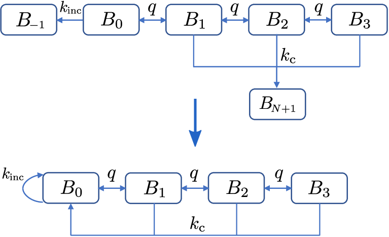
With and given, we are able to calculate the unconditioned mean escape time which is defined by
| (35) |
One can also apply the same arguments to as we used for and and seek instead of .
Another way to calculate was introduced by Hill [44]. He showed that the unconditioned mean escape time can be calculated if we consider the steady state in a transformed network without absorbing states. The transformed network is obtained by rewiring the transitions to absorbing states to the initial state in the original network. For instance, the maximum backtracking depth is set to be in Fig. 7, and all transitions to absorbing states are rewired to the initial state
The probability distribution of the stationary state of the rewired network can be found as , where , , , , and
The unconditioned mean escape time is given by
| (36) |
One should note that we can get for free by using Eq. (35) if we have the conditional incorporation time , the conditional cleavage time , the incorporation and cleavage probability , and . However, one cannot recover the conditional mean times and even if we know , , and because essentially, we are trying to solve and from [44]
which does not have a unique solution.
V.2 Mean conditional times for a trailing RNAP that advances
To derive the incorporation probability when the trailing RNAP is moving forward with elongation rate , we use Fig. 2 to build our solution. Let be the probability of incorporating the error, given that the RNAP start at state . Note that by definition, only makes sense for , where is the maximum backtracking depth, which is also the distance between the trailing and leading RNAP when the backtracking dynamics first started.
As a boundary condition, we have . This is because when the leading RNAP is at the realignment position and there is no room for backtracking, it can only incorporate the error and move forward. Suppose now we have for all , we can recursively build the solution for for via
| for all | ||||
| (37) |
We can use similar method as the previous section and study (numerically) the mean escape times. Let , where is the time to reach one of the absorption states, is the indicator function for the event and the subscript represents the initial state , with and . The stochastic equations are given by
| (38) |
The derivation for is similar. The linear system (37)-(38) can be easily solved since the size of the matrix in the linear system is on the order of the typical gap size between RNAPs during transcription. The mean time for a backtracking polymerase to incorporate the wrong nucleotide is when the initial distance from the trailing polymerase is . The corresponding mean time for a backtracking polymerase to cleave the wrong nucleotide is and the unconditioned mean escape time is . The above analyses provides an alternative methods for computing mean exit times and have been verified against the direct method presented in the main text.