Data-driven sensitivity analysis in surface structure determination using total-reflection high-energy positron diffraction (TRHEPD)Journal: Computer Physics Communications

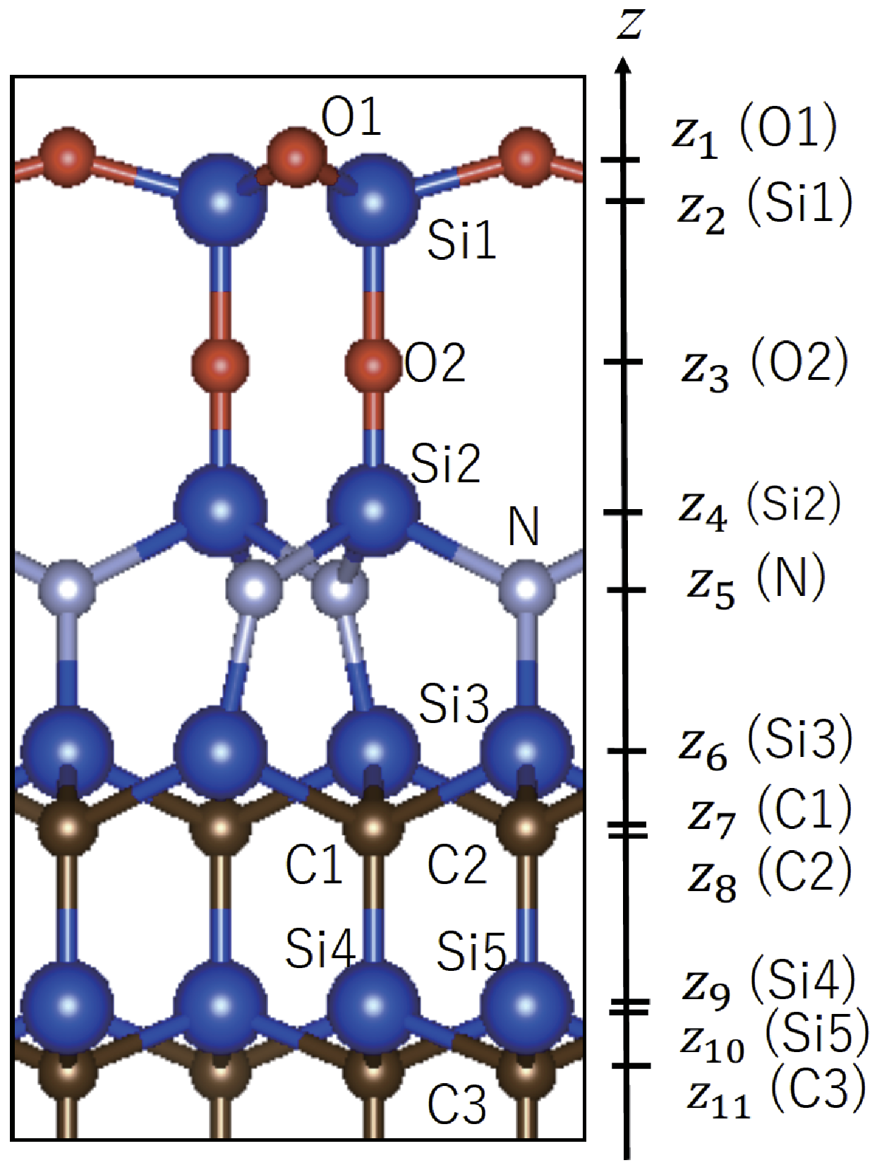
The surface measured by TRHEPD in the present work is Si₄O₅N₃ / 6H-SiC (0001)-($\sqrt{3}\times\sqrt{3}$) R30^∘ [8, 9, 10]. Figure 1 shows a side view of the structure reported in references  [8, 9, 10]. The $z$ axis is chosen to be perpendicular to the surface. The top view is found, for example, in Fig.1(c) of Ref.[10]. We restricted ourselves to the analysis of the TRHEPD data in the one-beam condition (see Sec. 3.2) which is sensitive only to the atomic coordinates perpendicular to the surface, $z$. The notation of the atomic sites in Fig. 1, such as O1, Si1 and O2, follows that in Ref. [10]. The $z$ coordinates of the sites are denoted as $z_{1}({\rm O1})$, $z_{2}({\rm Si1)}$, $z_{3}({\rm O2)}$, $z_{4}({\rm Si2)}$, $z_{5}({\rm N)}$, $z_{6}({\rm Si3)}$, $z_{7}({\rm C1)}$, $z_{8}({\rm C2)}$, $z_{9}({\rm Si4)}$, $z_{10}({\rm Si5)}$, and $z_{11}({\rm C3)}$ in the descending order ($z_{1}>z_{2}>....>z_{11}$).

The preparation of the sample (of size $5\times 10\,{\rm mm}^{2}$) was as follows. The epitaxial SiON layer was grown on an on-axis 4H-SiC(0001) substrate [8]. The substrate was initially etched with hydrogen gas under atmospheric pressure at 1623K for 15 min to clean and atomically smoothen the surface [15], and subsequently exposed to nitrogen gas at the same temperature. Oxygen gas was not intentionally introduced in this experiment but may have been mixed in the reactant as an impurity. Samples were then transferred to the TRHEPD measurement chamber and further annealed (973 K, 60 min) in UHV (less than $1.0\times 10^{-7}$ Pa) to remove surface contamination.

The details of the TRHEPD station at the KEK-IMSS-SPF are described elsewhere [6, 16, 17] and a brief overview is given below. A linac-based brightness-enhanced positron beam with an energy of 10 keV was used. The diffraction patterns were obtained under the one-beam condition [14, 4], where the beam azimuthal angle was set at 7.5^∘ off the $[11\bar{2}0]$ direction. In the one-beam condition, the diffraction spot intensity depends primarily on the atomic coordinates perpendicular to the surface because the in-plane diffraction is effectively suppressed. The dependence of the 00-spot diffraction intensity ($I_{00}^{\rm(exp)}(\theta)$) on the glancing angle ($\theta$) of incidence, called the rocking curve [14, 4], was extracted from the series of TRHEPD patterns acquired, taken with an exposure time of 1.5 min each. The glancing angle was varied from $\theta_{\rm min}=0.5^{\circ}$ to $\theta_{\rm max}=6.5^{\circ}$ in $\Delta\theta=0.1^{\circ}$ steps by tilting the sample. The experimental rocking curve was expressed as $F_{\rm exp}=(I^{\rm(exp)}_{00}(\theta_{1}=\theta_{\rm min}),...,I^{\rm(exp)}_{00}(\theta_{\nu}=\theta_{\rm max}))$, with $\nu\equiv 1+(\theta_{\rm max}-\theta_{\rm min})/\Delta\theta=61$. The experimental data and the corresponding calculated data were normalized as $|F_{\rm exp}|=\{\sum_{i}^{\nu}|I^{\rm(exp)}_{00}(\theta_{i})|^{2}\}^{1/2}=1$ and $|F_{\rm cal}|=\{\sum_{i}^{\nu}|I^{\rm(cal)}_{00}(\theta_{i})|^{2}\}^{1/2}=1$, respectively, when the R-factor (1) was calculated. Since only the data obtained in the one-beam condition were analyzed, the procedure described in the next subsection concerns only that with the $z$ coordinates $(X=(z_{1},z_{2},...))$.

The optimization procedure was carried out with the R-factor as the function of the eight coordinates, $\{z_{i}\}_{i=1,8}$ ($R=R(z_{1},z_{2},z_{3},z_{4},z_{5},z_{6},z_{7},z_{8})$. The eight coordinates were chosen so that the probed region consists of the whole SiON region ($z_{1},z_{2},z_{3},z_{4},z_{5}$) and a set of bulk SiC layers ($z_{6},z_{7},z_{8}$). The variables $z_{9},z_{10},z_{11}$ are fixed to be those in the initial structure, which are similar to the bulk positions. The calculated system contains a semi-infinite bulk region, as in the existing papers of TRHEPD measurement ([4] and references therein).

The iterative optimization procedure was made using the gradient-free, Nelder-Mead algorithm [19, 20] for which a Python code was developed in the previous work [1, 2]. The Nelder–Mead algorithm was performed by a module in the scipy library (scipy.optimize.fmin). Hereafter we use the notation $X$ specifically for the vector $X=(z_{1},z_{2},z_{3},z_{4},z_{5},z_{6},z_{7},z_{8})^{\rm T}$ in the eight-dimensional data space. In the Nelder-Mead algorithm, some of the set of $n+1(=9)$ sampling points $\{X^{(l)}\}^{[k]}(l=0,1...,8)$ are replaced by new points suitably found by calculation in every iteration, where $l$ is the sampling point index and $k$ is the iteration step index ($k=0,1,2...$). The best sampling point $X^{[k]}\equiv{\rm argmin}_{l}(\{R(X^{(l)})\}^{[k]}))$ is obtained in the course of the iteration. The iterative procedure is performed until the R-factor value converges within a given criteria of $\Delta R=5\times 10^{-4}$. The criteria value $\Delta R=5\times 10^{-4}$ is lower than the required threshold of magnitude, since an R-factor value less than 0.02 ($R(X)\leq 0.02$) is regarded as acceptable in the TRHEPD experiments noted at the beginning of the present section. Such a criteria value was used so as to demonstrate that even such a narrow convergence can be attained within short computational time. The initial data of the sampling points $\{X^{(l)}\}^{[k]}(l=0,1,2,...,8)$ is chosen by the researcher. The structure in Ref. [10] was chosen to be the initial data of the zero-th sampling point $X^{[0](0)}=(z^{[0](0)}_{1},z^{[0](0)}_{2},...,z^{[0](0)}_{8})^{\rm T}$, as mentioned above. The initial data of the other sampling points $\{X^{(l)}\}^{[0]}(l=1,2,...,8)$ were chosen so that the $l$-th sampling point $X^{(l)[0]}=(z^{(l)[0]}_{1},z^{(l)[0]}_{2},...,z^{(l)[0]}_{8})^{\rm T}$ is displaced by $0.05$ Å  from the zero-th sampling point $X^{[0](0)}$ only in the $l$-th coordinate ($z^{(l)[0]}_{l}=z^{(0)[0]}_{l}+0.05$Å, $z^{(l)[0]}_{i}=z^{[0](0)}_{i}$ for $i\neq l$).

The optimization procedure with the Nelder-Mead algorithm converged at the 42-th iteration. This took the computational time, $T$, of approximately one minute of one CPU of the Oakforest-PACS. The R-factor values for the initial and converged structures were $R^{\rm(ini)}=R(X^{\rm(ini)})=2.28\times 10^{-2}$ and $R^{\ast}=R(X^{\ast})=0.91\times 10^{-2}$, respectively. The converged point was $X^{\ast}=(z_{1}^{\ast},z_{2}^{\ast},...,z_{8}^{\ast})\approx$ (9.09Å, 8.67Å, 7.03Å, 5.60Å, 4.80Å, 3.11Å, 2.64Å, 2.44Å). The difference between the initial and converged structures ($\delta z_{i}\equiv z_{i}^{\ast}-z_{i}^{\rm(ini)}$) was ($\delta z_{1}$, $\delta z_{2}$, $\delta z_{3}$, $\delta z_{4}$, $\delta z_{5}$, $\delta z_{6}$, $\delta z_{7}$, $\delta z_{8}$) $\approx$ (-0.10Å, 0.00Å, -0.01Å, 0.15Å, -0.03Å, 0.00Å, 0.01Å, 0.00Å).

Figure 2 shows the calculated rocking curves $F_{\rm cal}$ in the initial and converged structures, together with the experimental data $F_{\rm exp}$. The calculated rocking curves $F_{\rm cal}$ in the converged structure agrees with the experimental data $F_{\rm exp}$ more closely than the rocking curve of the initial structure. Note that TRHEPD technique is sensitive to the small difference ($|\delta z_{i}|\leq 0.15$Å). While it is certain that the structure of the present specimen is essentially the same as that in the previous papers [8, 9, 10], it would be of interest to see whether the variation in the sample preparation procedure produced this small difference.

The sensitivity analysis was carried out after the optimization, by capturing the numerical behavior of $R(X)$ near the converged point $X^{\ast}$. We used supercomputers to compute $R(X)$ on the local grid of the coordinates $z_{i}\equiv z_{i}^{\ast}+mh$ for $m=-3,-2,-1,0,1,2,3$ and $i=1,...,8$ with the uniform grid interval $h=0.05$ Å. The total number of eight-dimensional grid points was $N_{\rm grid}=7^{8}=5,764,801$. Although the total operational cost on the grid points is large, a fast computation is possible on modern massive parallel supercomputers. The parallelism was carried out with Message Passing Interface (MPI) and each CPU executed one MPI process. The total computational time $T$ with the $N_{\rm grid}$ grid points was approximately 1.5 hours using $N_{\rm CPU}=2,048$ CPUs of Oakforest-PACS. Each CPU calculated the R-factor $R(X)$ at approximately $N_{\rm grid}/N_{\rm CPU}\approx 2815$ grid points.

Figure  3 demonstrates the anisotropic sensitivity among a few two-dimensional isovalue plots of $R=R(z_{1},z_{2},...,z_{8})$ on the local grid with the use of color-coding. Figure  3(a) is the isovalue plot on the $z_{1}$-$z_{2}$ plane, where all the other variables are fixed to be the converged values ($z_{i}=z_{i}^{\ast}$ for $i=3-8$). We found that the function $R(X)$ is quite sensitive to the deviation in the $(1,-1,0,0,0,0,0,0)^{\rm T}$ direction, being proportional to the distance of the two atomic layers $(z_{1}-z_{2})$, therefore showing that there is a significant contribution to the diffraction signal by the interaction of the positron waves scattered from the two atomic layers $z_{1}$ and $z_{2}$. Figure  3(b) is the isovalue plot on the $z_{1}$-$z_{8}$ plane showing that the function $R(X)$ is insensitive to the deviation in the $(0,0,0,0,0,0,0,1)^{\rm T}$ direction or the $z_{8}$-axis direction. Figure  3(c) is the isovalue plot on the $z_{7}$-$z_{8}$ plane and indicates that the function $R(X)$ is insensitive to any deviation on the $z_{7}$-$z_{8}$ plane. These properties are consistent with surface selectivity or the statement that the TRHEPD measurement observes mainly the shallow region with $z\geq z_{6}$.

The anisotropic behavior of the function $R(X)$ was systematically examined by the variance-covariance matrix $S$, whose $(i,j)$ component is defined as

for $i,j=1,2,...,8$ with the weight function

and the normalization factor

A parameter $s=0.002$, called the scaling parameter, is introduced, which is the tolerance measure of the uncertainty for the R-factor value.

It is noteworthy that the function $R(X)$ can be written formally by the second-order Taylor expansion

with $\Gamma_{ij}\equiv\partial^{2}(Rs^{-1})/(\partial z_{i}\partial z_{j})$ of the curvature matrix $\Gamma$. If the third- and higher-order terms of the Taylor expansion are ignored, the inverse matrix of $S$ is the curvature matrix $\Gamma$ ($S=\Gamma^{-1}$). The isovalue plot of Eq. (5) ($R(X)={\rm(constant)}$) forms an $n$-dimensional ellipsoid and the $k$-th eigenvector $\bm{v}_{k}$ indicates a principal axis of the $n$-dimensional ellipsoid.

When the integrals in Eq. (2) and Eq. (4) are reduced to the sum over the local grid points defined at the beginning of this section, the matrix $S$ was obtained as

in units of $10^{-3}$ Ų. The matrix, $S$, is symmetric and Eq. (15) shows only the upper triangular elements explicitly. The importance of the off-diagonal elements is characterized by the quantity $q_{i}\equiv(\sum_{j\neq i}|S_{ij}|)/|S_{ii}|$ for each column ($i=1,2,...,8$). The values were $q_{1}=1.87,q_{2}=1.94,q_{3}=1.04,q_{4}=1.43,q_{5}=0.54,q_{6}=0.45,q_{7}=0.19,q_{8}=0.08$. It was found that the off-diagonal elements are significant among the first to fifth columns ($q_{i}\geq 0.5$ for $i=1,...,5$). The presence of the significant off-diagonal elements in S indicates that the effect of the displacement of each atomic layer correlates significantly to the value of the R-factor in the first to fifth layers.

The principal deviation direction in the eight-dimensional data space is obtained by solving the $8\times 8$ matrix eigenvalue equation

with $0\leq\lambda_{1}\leq\lambda_{2}\leq...\leq\lambda_{8}$ and $|\bm{v}_{k}|=1$. The $k$-th eigenvalue $\lambda_{k}$ indicates the directional variance in the $\bm{v}_{k}$ direction. The values were $\lambda_{1}=0.73\times 10^{-3}$Ų, $\lambda_{2}=4.53\times 10^{-3}$Ų, $\lambda_{3}=6.18\times 10^{-3}$Ų, $\lambda_{4}=8.20\times 10^{-3}$Ų, $\lambda_{5}=9.62\times 10^{-3}$Ų, $\lambda_{6}=9.92\times 10^{-3}$Ų, $\lambda_{7}=11.3\times 10^{-3}$Ų, $\lambda_{8}=18.7\times 10^{-3}$Ų. The sum of the eigenvalues ${\rm Tr}[S]=\sum_{k=1}^{8}\lambda_{k}$ quantifies the total uncertainty and the difference between the eigenvalues indicates the anisotropy in the uncertainty. For example, the first eigenvector $\bm{v}_{1}$ with the smallest eigenvalue (directional variance) ${\lambda_{1}}$ represents the most sensitive direction or the direction with the smallest uncertainty.

Figure 4 shows the values of the eigenvector components $\bm{v}_{k}=(v_{1k},v_{2k},..,v_{8k})^{\rm T}$ for $k=1,2,...,8$ revealing the principal axis directions for the anisotropic sensitivity. As an example, the first eigenvector $\bm{v}_{1}$ is approximated to be $\bm{v}_{1}\approx(1/\sqrt{2})(1,-1,0,0,0,0,0,0)^{\rm T}$ and thus the function $R(X)$ should be quite sensitive to the deviation in the $(1,-1,0,0,0,0,0,0)^{\rm T}$, as seen on Figure  3(a). As another example, the sixth and seventh eigenvectors are similar to the eighth and seventh original axis vectors ($\bm{v}_{6}\approx(0,0,0,0,0,0,0,1)^{\rm T},\bm{v}_{7}\approx(0,0,0,0,0,0,1,0)^{\rm T}$), respectively, which indicates that almost no interacting wavefunction is formed by the scattering process at the seventh and eighth atomic layers and so the variables $z_{7}$ and $z_{8}$ are barely correlated to the other variables. Thus the function $R(X)$ may be almost unchanged on the $(z_{7},z_{8})$ plane, as seen on Figure  3(c). In addition, it is also noted that $\bm{v}_{8}\approx(1/\sqrt{5})(1,1,1,1,1,0,0,0)^{\rm T}$ in Figure 4(h), which means that the function $R(X)$ is hardly affected by the constant shift among $z_{1},z_{2},z_{3},z_{4}$ and $z_{5}$ ($z_{i}\Rightarrow z_{i}+\alpha$ for $i=1,...,5$). In other words, the function $R(X)$ is contributed to mainly by the relative positions between the atoms within the slab region that contains the first to fifth layers.

The above sensitivity analysis implies that the optimization analysis with the six variables ($z_{1}$, $z_{2}$, $z_{3}$, $z_{4}$, $z_{5}$, $z_{6}$) would give a reasonable result. Thus, we performed the optimization analysis with these six variables. The calculated system is a slab that consists only of the eleven layers at $z=z_{1},....,z_{11}$ in Figure 1, and neglecting the bulk part, since it has been shown that the R-factor for TRHEPD seems not to be sensitive (or hardly at all) to the atomic positions of the deeper layers ($z<z_{11}$). The variables $z_{7},z_{8},z_{9},z_{10},z_{11}$ are fixed to be those in the initial structure.

The optimization procedure converged at the 32-nd iteration. The converged point was $X^{\ast}=(z_{1}^{\ast},z_{2}^{\ast},...,z_{6}^{\ast})\approx$ (9.12 Å, 8.69 Å, 7.08Å, 5.58Å, 4.76Å, 3.09Å). The R-factor value at the converged structure was $R^{\ast}=R(X^{\ast})=0.97\times 10^{-2}$. The difference in the initial and converged structure ($\delta z_{i}\equiv z_{i}^{\ast}-z_{i}^{\rm(ini)}$) was ($\delta z_{1}$, $\delta z_{2}$, $\delta z_{3}$, $\delta z_{4}$, $\delta z_{5}$, $\delta z_{6}$) $\approx$ (-0.07Å, 0.02Å, 0.04Å, 0.13Å, -0.07Å, -0.02Å). Figure 5 shows the calculated rocking curves for the converged structures by the six-variable optimization procedure (dotted line), together with that by the former eight-variable optimization procedure (solid line) and the experimental data (open circles). The difference in the converged coordinates between the eight- and six-variable analyses was (-0.03 Å, -0.02 Å, -0.05 Å, 0.02 Å, 0.04 Å, 0.02 Å) for $(z_{1}^{\ast},z_{2}^{\ast},...,z_{6}^{\ast})$. Since the eight and six-variable optimization procedures give only a small difference between the resulting converged structure and the rocking curves, we concluded that both optimization procedures are acceptable.

The present sensitivity analysis gives a guide for the valid practical choice of a set of variables, in terms of both computational cost and reliability.

Finally, we comment on the generality of the above data-driven sensitivity analysis. The sensitivity analysis gives a foundation for the appropriate choice of the variable set $X$ by solving the eigenvalue equation of the variance-covariance matrix. For example, if a material contains light and heavy atoms, the TRHEPD diffraction signal tends to be more sensitive to a heavy atom than to a light atom. For such cases, it is not trivial to choose an appropriate set of variables because a heavy atom at a deeper layer may make a larger contribution to the diffraction signal than a light atom at a shallower layer. Also, the analysis method can handle variables of different physical dimension at the same time, such as the position and the coverage (occupation fraction) of each surface atom. We hope to apply this method to other experiments for two-dimensional structures, such as those using surface X-ray diffraction (SXRD), low energy electron diffraction (LEED), low energy positron diffraction (LEPD) [21, 22].

It should be noted that a grid-based calculation is a rigorous global-search method but may incur a high computational cost with a large data dimension. The total computational cost of the grid-based calculation is proportional to the number of the grid points $N_{\rm grid}$. We should recall that the calculation on the eight-dimensional grid in Sec. 4.2 requires $N_{\rm grid}=7^{8}=5,764,801$ grid points and takes 1.5 hours using a quarter of the Oakforest-PACS supercomputer. The grid-based calculation on the ten-dimensional grid requires $N_{\rm grid}=7^{10}=282,475,249$ grid points and is estimated to take approximately one day using the whole system. Occupying the whole system for more than one day, however, is not usually allowed. In such a high-dimensional case, the Monte Carlo sampling method is promising both in the optimization procedure and the numerical integration such as Eq. (2). There are already research examples [23, 24] in which the Monte Carlo method has been used for the analysis of SXRD data, though the sensitivity analysis with the eigenvalue problem in Eq. (16) was not performed. Furthermore, it would be desirable to utilize the parallelizable Monte Carlo method [25] that can efficiently use massively parallel supercomputers.

References

- [1] K. Tanaka, T. Hoshi, I. Mochizuki, T. Hanada, A. Ichimiya, T. Hyodo, Acta. Phys. Pol. A 137 (2020) 188.
- [2] K. Tanaka, I. Mochizuki, T. Hanada, A. Ichimiya, T. Hyodo, T. Hoshi, jJAP Conf. Series, in press; Preprint:https://arxiv.org/abs/2002.12165/. arXiv:2002.12165.
- [3] C. Hugenschmidt, Surf. Sci. Rep. 71 (2016) 547.
- [4] Y. Fukaya, A. Kawasuso, A. Ichimiya, T. Hyodo, J. Phys. D 52 (2019) 013002.
- [5] Y. Fukaya, Chapter 4 - Diffraction: Determination of atomic structure, in: I. Matsuda (Ed.), Monatomic Two-Dimensional Layers, Micro and Nano Technologies, Elsevier, 2019, pp. 75 – 111.
- [6] I. Mochizuki, H. Ariga, Y. Fukaya, K. Wada, M. Maekawa, A. Kawasuso, T. Shidara, K. Asakura, T. Hyodo, Phys. Chem. Chem. Phys. 18 (2016) 7085.
- [7] Y. Endo, Y. Fukaya, I. Mochizuki, A. Takayama, T. Hyodo, S. Hasegawa, Carbon 157 (2020) 857.
- [8] T. Shirasawa, K. Hayashi, S. Mizuno, S. Tanaka, K. Nakatsuji, F. Komori, H. Tochihara, Phys. Rev. Lett. 98 (2007) 136105.
- [9] T. Shirasawa, K. Hayashi, H. Yoshida, S. Mizuno, S. Tanaka, T. Muro, Y. Tamenori, Y. Harada, T. Tokushima, Y. Horikawa, E. Kobayashi, T. Kinoshita, S. Shin, T. Takahashi, Y. Ando, K. Akagi, S. Tsuneyuki, H. Tochihara, Phys. Rev. B 79 (2009) 241301(R).
- [10] S. Mizuno, T. Matsuo, T. Nakagawa, Surf. Sci. 661 (2017) 22.
- [11] A. Ichimiya, in: Positrons at Metallic Surfaces, Vol. 28 of Solid State Phenomena, Trans Tech Publications Ltd, 1992, pp. 143–148.
- [12] A. Kawasuso, S. Okada, Phys. Rev. Lett. 81 (1998) 2695.
- [13] A. Ichimiya, Jpn. J. Appl. Phys. 22 (1983) 176.
- [14] A. Ichimiya, Surf. Sci. Lett. 192 (1987) L893.
- [15] H. Nakagawa, S. Tanaka, I. Suemune, Phys. Rev. Lett. 91 (2003) 226107.
- [16] K. Wada, T. Hyodo, A. Yagishita, M. Ikeda, S. Ohsawa, T. Shidara, K. Michishio, T. Tachibana, Y. Nagashima, Y. Fukaya, M. Maekawa, A. Kawasuso, Eur. Phys. J. D 66 (2012) 37.
- [17] M. Maekawa, K. Wada, Y. Fukaya, A. Kawasuso, I. Mochizuki, T. Shidara, T. Hyodo, Eur. Phys. J. D 68 (2014) 165.
- [18] T. Hanada, H. Daimon, S. Ino, Phys. Rev. B 51 (1995) 13320.
- [19] J. A. Nelder, R. Mead, The Computer Journal 7 (1965) 308.
- [20] M. Wright, Direct search methods: Once scorned, now respectable, in: D. Griffiths, G. Watson (Eds.), Numerical analysis, Addison-Wesley, 1996, pp. 191–208.
- [21] S. Y. Tong, Surf. Sci. 457 (2000) L432.
- [22] K. Wada, T. Shirasawa, I. Mochizuki, M. Fujinami, M. Maekawa, A. Kawasuso, T. Takahashi, T.Hyodo, e-J. Surf. Sci. Nanotechnol. 16 (2018) 313.
- [23] M. Anada, Y. Nakanishi-Ohno, M. Okada, T. Kimura, Y. Wakabayashi, J. Appl. Cryst. 50 (2017) 1611.
- [24] M. Anada, K. Kowa, H. Maeda, E. Sakai, M. Kitamura, H. Kumigashira, O. Sakata, Y. Nakanishi-Ohno, M. Okada, T. Kimura, Y. Wakabayashi, Phys. Rev. B 98 (2018) 014105.
- [25] K. Hukushima, Y. Iba, AIP Conf. Proc. 690 (2003) 200.