Multi-Source Domain Adaptation with Collaborative Learning for Semantic Segmentation
Abstract
Multi-source unsupervised domain adaptation (MSDA) aims at adapting models trained on multiple labeled source domains to an unlabeled target domain. In this paper, we propose a novel multi-source domain adaptation framework based on collaborative learning for semantic segmentation. Firstly, a simple image translation method is introduced to align the pixel value distribution to reduce the gap between source domains and target domain to some extent. Then, to fully exploit the essential semantic information across source domains, we propose a collaborative learning method for domain adaptation without seeing any data from target domain. In addition, similar to the setting of unsupervised domain adaptation, unlabeled target domain data is leveraged to further improve the performance of domain adaptation. This is achieved by additionally constraining the outputs of multiple adaptation models with pseudo labels online generated by an ensembled model. Extensive experiments and ablation studies are conducted on the widely-used domain adaptation benchmark datasets in semantic segmentation. Our proposed method achieves 59.0% mIoU on the validation set of Cityscapes by training on the labeled Synscapes and GTA5 datasets and unlabeled training set of Cityscapes. It significantly outperforms all previous state-of-the-arts single-source and multi-source unsupervised domain adaptation methods.
1 Introduction

Semantic segmentation as one of the core tasks in computer vision community, aims to assign semantic label to each pixel of images, e.g., person, car, road and etc.. With the development of convolutional neural networks (CNNs), semantic segmentation has made great progress recently. For example, recent deep methods [2, 6, 8, 13, 43], have achieved superior performance on almost all public benchmarks. However, their success is based on the large numbers of densely annotated images which used to train the networks. Dense pixel-level annotation for semantic segmentation is very laborious and expensive, e.g., annotating one image in the Cityscapes dataset [5] takes about 90 minutes, which makes it difficult and sometimes even impossible to collect large amounts of densely annotated images for semantic segmentation. Thanks to the recent progress in graphics and simulation infrastructure, simulators can generate lots of images with dense annotation for semantic segmentation, such as recent proposed large-scale dense labeled datasets SYNTHIA [31], GTA5 [30] and Synscapes [38]. Although the huge amounts of annotated synthesized images are very close to the real scene, there is still great domain gap between synthetic datasets and real scene datasets. The domain gap causes another problem that networks trained on synthetic datasets often perform poorly on real target scenes. To handle this issue, many un-/semi-supervised domain adaptation (UDA) approaches are proposed, like [15, 24, 3, 12, 33, 37, 39] and etc., with the purpose of mitigating the gap between synthetic source and real target domain. Over the past years, UDA has made a great progress.
Although existing works have greatly boosted the performance of UDA for semantic segmentation, most of them focus on single source. Seldom works consider a more practical setting where labeled datasets from multiple sources with different distributions are available, e.g., SYNTHIA and GTA5. Training with multiple sources can further alleviate the problem on lack of annotated data. Moreover, multiple sources sampled from different distribution can also encourage networks to learn more essential knowledge for semantic segmentation. A straightforward approach is to simply combine all source domains into a single one, and then trains a UDA model on the combined sources and target domain dataset. This simple method can indeed boost the performance, but it does not fully exploit the abundant information across multiple source domains. Domain shift across multiple sources restricts the power within them in learning a more powerful domain adaptation model.
There are several multi-source deep UDA methods are proposed recently to exploit multiple source domains for better adaptation. They align different domains by translating images from source domains to the target style via generative adversarial networks (GAN). However, most of them [26, 32, 17] work on image classification task except for MADAN [45] which works on semantic segmentation, a pixel-wise prediction task. In this paper, we propose an approach based on collaborative learning and image translation to address multi-source domain adaptation for semantic segmentation.
Our observation shows that appearance discrepancy especially color discrepancy between source domains and target domain has a great impact on the performance of adaptation. Existing works [35, 14, 40, 11] demonstrate that style transfer could reduce this discrepancy in some extent. However, most of them are complicated to plug in networks during training process. Therefore, we propose a simple image translation method to first mitigate domain gap between sources and target. Unlike MADAN [45], FDA [39] and GAN-based translation methods, we propose to translate source domain images to the target style by aligning different distributions to the target domain in LAB color space. In addition, we observe that apart from discrepancy in appearance, images from different domains do still share much similarity in semantic contexts as shown in Fig 1. The shape of instances (person, car, bike and etc.) and spatial layout of different instances (cars always on the road, sidewalk adjacent to the road, sky on the top and etc.) are almost the same in all domains. Two collaborative learning strategies are proposed to explore essential and domain-invariant semantic contexts across different domains. First we propose a collaborative learning between source domains to investigate the case of domain adaptation without seeing any data from target domain, which is also called domain generalization in previous works [7, 25, 42]. For each source domain, we have a semantic segmentation network supervised by annotation maps, and an additional soft supervision coming from other models trained on a different source domain. In addition, similar to previous UDA methods [45, 39], we also consider making full use of the unlabeled data of the target domain to further boost the performance. A collaborative learning based on target domain is proposed, in which an ensemble of models trained on source domains is used to produce pseudo labels for data from target domain in an online fashion. In turn, each model can be additionally supervised by the generated pseudo labels. Such two collaborations help constantly improve each model’s adaptation capability to target domain during the training process.
The performance of our method significantly outperforms other state-of-the-art single-source and multi-source UDA methods. This success of proposed method is mainly attributed to the effective image translation and domain-invariant feature learning. Note that, our method can be trained in both end-to-end and stage-wise.
2 Related works
In this section, we briefly review some related works in the literature, i.e., semantic segmentation, domain generalization and unsupervised domain adaptation.
2.1 Semantic Segmentation
Semantic segmentation plays a vital role in computer vision community and is beneficial to many practical applications, such as autonomous driving, virtual reality and medical imaging and etc.. It has developed several decade years and is well researched. Since Long et al. [18] propose to transform the classification CNNs to fully convolutional network for semantic segmentation, large numbers of deep learning based methods have been proposed and greatly boost the advances of this task. For example, Chen et al.propose the DeepLab series [1, 2] approaches which utilize átrous spatial pyramid pooling (ASPP) to capture different scale of context information. Fu et al. [6] involve non-local attention block into the CNNs architecture to exploit the global context of image and relation of objects. Hou et al. [10] propose a new effective strip pooling to model long-range dependencies. However, the advanced performance of these semantic segmentation methods often build on the large amounts of densely annotated images which are usually hard and sometimes impossible to collect.

2.2 Domain Generalization
Domain generalization is a particular case of transfer learning. It’s purpose is to enhance the generalization ability of models on new domains that have not been seen during the training process. Currently, most of the domain generalization methods can be categorized to three parts: data-based, feature-based and meta-learning based. Most data-based methods employ GANs, Variational Autoencoder (VAE) or other image edit methods to generate new data for network training to enhance robustness and generalization of the models, e.g., Dlow [7] and STRG [41]. Then, the feature-based methods mainly aim to learn representations invariant to different domains by adversarial learning to align features or employing normalization to eliminate the style information, like CADAG [28] and IBN-Net [25]. Meta-learning based methods aim to enhance the generalization ability by using meta learning, such as Zhang et al. [42] deal with the domain generalization from the training scheme perspective and develop a target-specific normalization method to further boost the generalization ability in unseen target domain. Domain generalization do not access the data in target domain which may not learn the optimal feature for target domain.
2.3 Unsupervised Domain Adaptation
In contrast to domain generalization, unsupervised domain adaptation involves in unlabeled data of target domain during training process to learn knowledge of it. UDA has developed many years and large numbers of methods have been proposed. From the perspective of the number of source domains, domain adaptation methods can be split into two categories: single-source and multi-source.
Single-source domain adaptation focuses on single-source-single-target setting. Most of existing UDA works are for classification, like MMD [19, 20], ADDA [34] and et al.. With the synthetic dataset GTA5, SYNTHIA and Synscapes proposed , UDA for semantic segmentation has also achieved great advances in recent. For example, Tsai et al. [33] propose AdaptSeg that based on adversarial learning to aligns scene layout and local context of images between source and target domain. Yang et al. [39] draw on the image-to-image translation and propose to using Fourier Transform to translate images in source domain to the style of target domain. While Li et al. [15] propose a bidirectional framework for domain adaptation and learn a image translation model with perceptual loss to translate images to target style. These methods have significantly boost the performance of UDA in semantic segmentation. However, they do not take the existing multiple different source domains into account which is a great waste of labeled resources.
Multi-source domain adaptation aims to make full use of existing labeled source for adaptation. Compared to single-source UDA, it is relatively more challenging because of the shift between source domains. There are also some multi-source UDA works but most of them focus on image classification. Directly extending these methods for semantic segmentation may not work. Zhao et al. [45] propose MADAN for semantic segmentation. They first learns a cycle GAN [46] for each source domain to translate images to target, and then combine different adapted sources with specific weights. Finally, training a adaptation network on the combined data in a way similar to single-source UDA. In contrast to [45], we not only draw on the style-transfer for image-to-image translation, also aim to learn the shared semantic information of source domains and explore the knowledge of unlabeled target data.

3 Proposed Approaches
3.1 LAB-based Image Translation
We observe that the domain discrepancy between domains mainly lies in appearance of images, i.e., color and texture. For example, the appearance discrepancy between source domains (GTA5 and SYNTHIA), and between source domains and target domain (GTA5 and Cityscapes) as demonstrated in Fig. 1. This discrepancy would further increase the difficulty of multi-source domain adaptation. An effective style transfer could reduce this discrepancy to some extent. For simplicity and efficiency, we proposed an image translation method that translates the style of images in source domains to the style of target domain by aligning the distribution of pixel values, like [29]. Specifically, due to the gamut of LAB color space is larger than RGB color space, and the style of images translated on LAB color space are closer to the style of images in target domain than directly operated on RGB color space as shown in Fig. 3, we involve the image translation based on LAB color space to achieve the target of reducing domain discrepancy.
Specifically, for a RGB image in source domains, it is firstly converted to LAB color space to generate LAB image , . Then, we calculate the mean and standard deviation values of each channel of the generated LAB image . At the same time, an image from target domain is randomly selected and converted to LAB color space in same way as image from source. After that, we also calculate the mean and standard deviation values of this converted target image. Finally, we translate the converted LAB image from source domains to the style of target by shifting the distribution of pixel values to the image of target domain, ie.,
| (1) |
After aligning distribution in LAB color space, we then convert the translated LAB image from source domains back to the RGB color space , , for the subsequent training. The and are the library conversion function in python, and also easy to implement it with CUDA to accelerate computation. Fig 3 shows the qualitative comparison between RGB- and LAB-based translation. We can see that the images after translation are closer to the style of target domain, which the gap between domains is reduced to some extent. Moreover, the LAB-based translated images are closer to the style of target images.
3.2 Collaborative Learning between Labeled Source Domains
As shown in Fig. 1, although the images of different source domains are sampled from different simulators, i.e., from different i.i.d distributions, they are highly structured and share many similarities, e.g., the spatial layout of different categories and local context of objects. Based on this observation and to encourage models learn these essential similar properties for semantic segmentation, we propose a collaborative learning (Co-Learning) method which fully takes advantage of the capacity of different models learned on different source domains. This approach utilizes a model learn from one source domain to teach the model trained on another one, which allows that model to learn the knowledge from current source domain.
Assume that there are different labeled source domains which are sampled from different i.i.d distributions, and deep neural networks of the same architecture but different weights learned on these source domains. Then, for an model , the learning process of model is supervised by segmentation loss on labeled data from source and collaborative loss on output from source . That is, for model , the object function is
| (2) |
where the loss is the cross entropy loss, i.e.,
| (3) |
and the loss is the average of Kullback-Leibler (KL) divergence loss, i.e.,
| (4) |
| (5) |
are the input image, outputs of networks and the corresponding ground truth respectively. For , the subscript indicates that is generated by while the superscript indicates is the feature computed for images from domain , i.e., . is the number of categories to be segmented, indicates the softmax function, represents the number of pixels in image . Collaborative learning can allow the model learn the knowledge of other models learned from corresponding source . Thus, rather than stuck in the source domain , model also tries to learn essential properties between all the source domains for better generalization and segmentation on target domain.
Difference with existing works: In the co-training of CLAN [21] and CT [27], two diversified classifiers are produced to make predictions and their ensemble with either summation or multiplication is taken as the final prediction; however, in the collaborative learning framework, two segmentation models trained based on each source domain teach each other to extract essential semantic information across domains. CrDoCo [4] uses bi-directional KL divergence to encourage segmentation consistency between images in unlabeled target domain and their source-style transformed correspondences. However, in our work, images from both source domains are first transformed to the same style, i.e., target domain style. Then an arbitrary image is sent to two models that are trained for source 1 and source 2 respectively. The prediction of the model trained for the source domain that image comes from works as teacher to supervise the other model’s prediction on the same image.
3.3 Collaborative Learning on Unlabeled Target Domain
In practice, unlabeled data is often relatively easy and cheap to collect. Moreover, models trained on the data of target domain can learn better features and perform well on target domain. Therefore, we propose a collaborative learning method to fully take advantage of the unlabeled images in target domain, and further boost the performance of models on target domain.
Denote target domain as which has collected large amounts of unlabeled images . For an image in the target domain , we first feed it to all the models and compute the corresponding outputs of models for the input image as , i.e., . Outputs of these networks are ensembled and a softmax function is used to compute the probability map, i.e.,
| (6) |
Finally, we generate one-hot pseudo labels for the target image by utilizing the probability map in a way similar to [15, 47], and the detail process is described in the Algorithm 1. After then, we can train models with both source domains and target domain. Thus, the object function for model becomes
| (7) |
where cross entropy loss is employed to compute the loss and is same as Equ. 3, the only difference is that the target labels are generated pseudo labels. Here the the weight term is designed to prevent poor predictions of the target image in early training process collapsing the network training, and represent current and maximum iterations of training process.
for c 0 to do 1
get the number of pixels which are predicted to category : ;
get the threshold that used to filter the prediction: ;
;
;
. end for 2
3.4 Network Architecture and Training
The overall architecture of proposed approach are shown in Fig. 2. In summary, it consists of three parts, i.e., image-to-image translation based on LAB color space, collaborative learning between labeled source domains and on unlabeled target domain. Firstly, images of source domains are translated to the style of target domain as described in Sec. 3.1 during training process. Note that for simplicity, we just showcase the collaborative learning approach for multi-source domain adaptation with two source domains. As shown in Fig. 2, we train a segmentation network, e.g., DeepLab v2 [1], for each source domain. These networks can be trained end-to-end which initialized from ImageNet pretrained model, or trained with stage-wise which initialized from source fine-tuned model. For each network, the final overall object function is as follows,
| (8) |
The loss ensures the correct functionality of networks for segmentation, while the loss allows the network to learn the similarities that shared by source domains. In addition, the loss allows the network learn the property of target data. When network training get converged, we have two strategies to obtain the final model. One is to choose the model which achieves the best performance on target domain. The other is to keep all models, and ensemble their outputs when inference. Unless otherwise specified, all refer to the last case. The following section tests the validity of proposed approach.
| GTA5Cityscapes | |||
|---|---|---|---|
| Methods | Before | Trans | Diff. |
| Direct Transfer | 39.53 | 43.36 | 3.83 |
| AdaptSeg [33] | 41.32 | 43.66 | 2.43 |
| AdaptSeg-LS [33] | 43.11 | 45.95 | 2.84 |
| Advent [37] | 44.30 | 45.96 | 1.66 |
4 Experiments
4.1 Datasets
In this subsection, we briefly introduce the datasets used to validate our adaptation method, i.e., the widely used dataset Cityscapes [5], and recent proposed synthetic datasets GTA5 [30], SYNTHIA [31], and Synscapes [38].
Cityscapes [5] consists of 5,000 real-world urban traffic scene images with 20481024 resolution and dense-pixel annotation. This dataset is split to 2,975 for training, 500 for validation and 1,525 for testing. Cityscapes annotates 33 categories and 19 of them are used for training and evaluation. The training set without ground truth is used for training adaptation models and validation set for evaluation.
GTA5 [30] includes 24,966 dense annotated images that are synthesized from a game engine with the resolution of 19141052. Its ground-truth labels are consistent with Cityscapes [5]. In a way similar to previous works [15, 37], common categories between GTA5 and Cityscapes are used in all experiments.
SYNTHIA [31] is a large synthetic dataset that consists of photo-realistic frames rendered from a virtual city. In experiments, we use the SYNTHIA-RAND-CITYSCAPES [31] set for adaptation. It contains 9,400 images with a resolution of 1280760 which are annotated into 16 categories. Similar to GTA5, its annotation are also automatically produced and compatible with Cityscapes. Following previous works [39, 33, 37], we evaluate performance on 16 and 13 common categories between Cityscapes and SYNTHIA when SYNTHIA is used.
Synscapes [38] is a synthetic dataset that created using photo-realistic rendering techniques. It consists of 25,000 images at 1440720 resolution with 33 categories dense annotation and only 19 of them are used. Similarly, its annotations are compatible with Cityscapes. The style of Syncscapes is closer to Cityscapes than GTA5 and Synscapes.
4.2 Implementation Details
We implement our proposed approach with PyTorch and conduct experiments by adopting DeepLab-v2 [1] with ResNet-101 [9] as backbone. We report the performance of both initialization from ImageNet pretrained model and initialization from source pretrained model, which are respectively denoted as end-to-end and stage-wise training stratgies. Following prior works [39, 37, 33], all the networks are trained with stochastic gradient descent (SGD) optimizer. The initial learning rate and momentum are set to and 0.9, respectively, and the polynomial decay policy with power of 0.9 is adopted to adjust the learning rate. We set the batch size to 1 for all datasets during training because of memory limitation. The hyper-parameters in collaborative learning on target domain, and are set to 50% and 0.9, respectively. It indicates that we keep pixels that prediction probability within the top 50% or higher than 0.9 as true labels, and reminder are ignored. The weights and for collaborative learning losses are set to 0.5, 0.1 for end-to-end training and 9.5, 0.1 for stage-wise training. Following Advent [37], we set the number of maximum iterations to 250,000 but early stop at 120,000 iterations. Same as previous works [39, 37, 33, 24], the metric mean intersection-over-union (mIoU) is used to evaluate the performance of our proposed adaptation method.
| (a) | ||
|---|---|---|
| Model | E | S |
| 56.90 | 57.72 | |
| 56.65 | 57.81 | |
| 58.55 | 59.04 | |
| (b) | ||
|---|---|---|
| Methods | mIoU | Diff. |
| Data Combination | 51.56 | – |
| MLDG+TN [42] | 52.73 | 1.17 |
| Co-Learning-Src | 55.79 | 4.23 |
4.3 Ablation Study
In this subsection, extensive experiments on adaptation from GTA+Synscapes to Cityscapes are conducted to study the effectiveness of each component in the proposed approach.
Firstly, LAB-based image translation is applied to the state-of-the-art UDA methods in semantic segmentation, i.e., AdaptSeg [33] and Advent [37], to investigate the effectiveness of proposed image translation method. Table 1 is the performance comparison of previous UDA methods training on original and translated images. From the results, we can see that LAB-based image translation can greatly boost the performance of UDA methods for semantic segmentation. For example, LAB-based translation advances the performance of direct transfer from 39.38% to 43.36%, which improves about 3.83%. The performance of AdaptSeg and Advent are also significantly boosted, i.e., 2.43%, 2.84% and 1.66% for AdaptSeg, AdaptSeg-LS and Advent respectively. These results demonstrate that the proposed simple image translation method based on LAB color space is effective for UDA in semantic segmentation. It is easy to implement, with only a little additional computation and without any extra hyper parameter. Note that, all results are reproduced with the code provided by the authors.
| GTA5 + Synscapes Cityscapes | ||||
| LAB-based | Data | Co-Learning | Co-Learning | mIoU |
| Trans. | Comb. | between Src. | on Target | |
| ✓ | 51.59 | |||
| ✓ | 54.38 | |||
| 54.03 | ||||
| 56.03 | ||||
| 57.27 | ||||
| 58.55 | ||||
| Methods |
Appr. |
Source |
road |
sidewalk |
building |
wall |
fence |
pole |
light |
sign |
veg |
terrain |
sky |
person |
rider |
car |
truck |
bus |
train |
mbike |
bike |
mIoU |
|---|---|---|---|---|---|---|---|---|---|---|---|---|---|---|---|---|---|---|---|---|---|---|
| DT [33] | – | S | 81.8 | 40.6 | 76.1 | 23.3 | 16.8 | 36.9 | 36.8 | 40.1 | 83.0 | 34.8 | 84.9 | 59.9 | 37.7 | 78.5 | 20.4 | 20.5 | 7.8 | 27.3 | 52.5 | 45.3 |
| AdaptSeg [33] | Adv | 94.2 | 60.9 | 85.1 | 29.1 | 25.2 | 38.6 | 43.9 | 40.8 | 85.2 | 29.7 | 88.2 | 64.4 | 40.6 | 85.8 | 31.5 | 43.0 | 28.3 | 30.5 | 56.7 | 52.7 | |
| FDA [39] | ST | 93.6 | 58.1 | 84.0 | 30.4 | 29.2 | 39.0 | 43.1 | 51.7 | 85.9 | 28.8 | 86.9 | 64.0 | 45.7 | 84.7 | 30.4 | 36.5 | 28.5 | 34.4 | 62.4 | 53.5 | |
| Advent [37] | Adv | 92.2 | 51.3 | 85.0 | 40.8 | 31.2 | 39.0 | 42.5 | 42.5 | 86.5 | 46.1 | 84.8 | 65.2 | 39.0 | 87.0 | 32.6 | 49.0 | 29.5 | 28.6 | 50.0 | 53.8 | |
| UIA [24] | Adv | 94.0 | 60.0 | 84.9 | 29.5 | 26.2 | 38.5 | 41.6 | 43.7 | 85.3 | 31.7 | 88.2 | 66.3 | 44.7 | 85.7 | 30.7 | 53.0 | 29.5 | 36.5 | 60.2 | 54.2 | |
| DT [33] | – | G | 75.8 | 16.8 | 77.2 | 12.5 | 21.0 | 25.5 | 30.1 | 20.1 | 81.3 | 24.6 | 70.3 | 53.8 | 26.4 | 49.9 | 17.2 | 25.9 | 6.5 | 25.3 | 36.0 | 36.6 |
| AdaptSeg [33] | Adv | 86.5 | 25.9 | 79.8 | 22.1 | 20.0 | 23.6 | 33.1 | 21.8 | 81.8 | 25.9 | 75.9 | 57.3 | 26.2 | 76.3 | 29.8 | 32.1 | 7.2 | 29.5 | 32.5 | 41.4 | |
| Advent [37] | Adv | 89.4 | 33.1 | 81.0 | 26.6 | 26.8 | 27.2 | 33.5 | 24.7 | 83.9 | 36.7 | 78.8 | 58.7 | 30.5 | 84.8 | 38.5 | 44.5 | 1.7 | 31.6 | 32.4 | 45.5 | |
| UIA [24] | Adv | 90.6 | 36.1 | 82.6 | 29.5 | 21.3 | 27.6 | 31.4 | 23.1 | 85.2 | 39.3 | 80.2 | 59.3 | 29.4 | 86.4 | 33.6 | 53.9 | 0.0 | 32.7 | 37.6 | 46.3 | |
| PyCDA [16] | CL | 90.5 | 36.3 | 84.4 | 32.4 | 28.7 | 34.6 | 36.4 | 31.5 | 86.8 | 37.9 | 78.5 | 62.3 | 21.5 | 85.6 | 27.9 | 34.8 | 18.0 | 22.9 | 49.3 | 47.4 | |
| BDL [15] | ST | 91.0 | 44.7 | 84.2 | 34.6 | 27.6 | 30.2 | 36.0 | 36.0 | 85.0 | 43.6 | 83.0 | 58.6 | 31.6 | 83.3 | 35.3 | 49.7 | 3.3 | 28.8 | 35.6 | 48.5 | |
| FDA [39] | ST | 92.5 | 53.3 | 82.4 | 26.5 | 27.6 | 36.4 | 40.6 | 38.9 | 82.3 | 39.8 | 78.0 | 62.6 | 34.4 | 84.9 | 34.1 | 53.1 | 16.9 | 27.7 | 46.4 | 50.5 | |
| PIT [22] | RL | 87.5 | 43.4 | 78.8 | 31.2 | 30.2 | 36.3 | 39.9 | 42.0 | 79.2 | 37.1 | 79.3 | 65.4 | 37.5 | 83.2 | 46.0 | 45.6 | 25.7 | 23.5 | 49.9 | 50.6 | |
| Data Comb. | – | A | 85.1 | 36.9 | 84.1 | 39.0 | 33.3 | 38.7 | 43.1 | 40.2 | 84.8 | 37.1 | 82.4 | 65.2 | 37.8 | 69.4 | 43.4 | 38.8 | 34.6 | 33.2 | 53.1 | 51.6 |
| AdaptSeg [33] | Adv | 89.3 | 47.3 | 83.6 | 40.3 | 27.8 | 39.0 | 44.2 | 42.5 | 86.7 | 45.5 | 84.5 | 63.1 | 38.0 | 79.4 | 34.9 | 48.3 | 42.1 | 30.7 | 52.3 | 53.7 | |
| Advent [37] | Adv | 91.8 | 49.0 | 84.6 | 39.4 | 31.5 | 39.9 | 42.9 | 43.5 | 86.3 | 45.1 | 84.6 | 65.3 | 41.0 | 87.1 | 37.9 | 49.2 | 31.0 | 30.3 | 48.8 | 54.2 | |
| MDAN [44] | Adv | 92.4 | 56.1 | 86.8 | 42.7 | 32.9 | 39.3 | 48.0 | 40.3 | 87.2 | 47.2 | 90.5 | 64.1 | 35.9 | 87.8 | 33.8 | 48.6 | 39.0 | 27.6 | 49.2 | 55.2 | |
| MADAN [45] | Adv | 94.1 | 61.0 | 86.4 | 43.3 | 32.1 | 40.6 | 49.0 | 44.4 | 87.3 | 47.7 | 89.4 | 61.7 | 36.3 | 87.5 | 35.5 | 45.8 | 31.0 | 33.5 | 52.1 | 55.7 | |
| Ours-E | – | 94.2 | 61.8 | 86.7 | 47.7 | 34.1 | 39.3 | 44.6 | 34.2 | 87.2 | 49.6 | 89.7 | 65.6 | 38.1 | 88.2 | 48.1 | 63.0 | 41.9 | 39.2 | 59.2 | 58.6 | |
| Ours-S | – | 93.6 | 59.6 | 87.1 | 44.9 | 36.7 | 42.1 | 49.9 | 42.5 | 87.7 | 47.6 | 89.9 | 63.5 | 40.3 | 88.2 | 41.0 | 58.3 | 53.1 | 37.9 | 57.7 | 59.0 |
Because our method can be trained in different strategies and there are models in the framework, we then test the performance of each single model and the final ensemble one with different training strategies. All these results are based on the setting that adapting from GTA5Synscapes to Cityscapes. As shown in Table 2 (a), the performance of all models are significantly improved and the ensembled model achieves the best performance. Therefore, we only report the ensembled model’s performance later. The collaborative learning between source domains does not access to the unlabeled target data and therefore can be used to address the task of domain generalization. Table 2 (b) shows the performance comparison with the recent multi-source domain generalization method MLDG [42] and a baseline based on simple data combination. We can see that collaborative learning achieves better generalization performance. For example, MLDG only marginally outperforms the simple baseline about 1.17%, while collaborative learning boosts the performance about 4.23%. Note that, collaborative learning here is only applied to source domains without image translation for fair comparison.
Table 3 shows different contribution of each component to performance of our proposed approach. As the results shown, training on combination of source domains can improve the performance on target domain to some extent, which achieves 51.59% and 54.38% respectively. Collaborative learning between different source domains further boosts the performance to 56.03%. Collaborative learning on target domain also boosts the performance on target which achieves 54.03%. This result shows that collaborative learning between source domains brings more improvements than on target domain. Moreover, full version of our approach achieves the best performance, achieving 58.55% on target domain. Thus, we can conclude that the proposed approach is effective for unsupervised domain adaptation in semantic segmentation.
4.4 Comparison with SOTA
In this subsection, our proposed approach is compared to the recent state-of-the-art single-source and multi-source UDA methods on the GTA5Synscapes to Cityscapes, including a baseline of source-only direct transfer (DT), single-source UDA methods [33, 24, 37, 16, 15, 39, 22], the multi-source baseline that simple combination of source domains and multi-source UDA methods [44, 45]. We further validate the effectiveness of our proposed method by conducting experiments based on adapting different number of source domains to target domain.
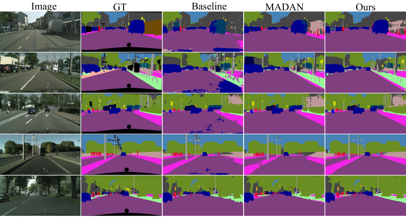
Table 6 shows the results comparison with other methods and Fig. 4 demonstrates the visual comparison with baseline and MADAN [45]. From the results of Table 6, we can see that simply combining the images of source domains for networks training can already greatly boost the generalization performance on target domain, which advances from the 44.1% of GTA5Cityscapes and 45.3% of SynscapesCityscapes to 51.6%. Simply adapting UDA methods to train on combination of source domains does not bring much improvements, such as AdaptSeg has only 1% improvement and Advent only 0.5%. By employing adaptation strategy, multi-source UDA further boost the performance, i.e., MDAN [44] achieves 55.2% and MADAN [45] achieves 55.7%. By further integrating collaborative learning on the source domains and target domain, we achieve 58.6% mIoU with the end-to-end training strategy and 59.0% mIoU with stage-wise training strategy, which
| sources | mIoU19 | mIoU16 | mIoU13 | |
|---|---|---|---|---|
| Source-Only | G | 39.53 | 43.28 | 48.25 |
| S | 44.43 | 48.74 | 54.09 | |
| Y | – | 32.31 | 37.41 | |
| Multi-Sources | GS | 59.04 | 61.25 | 65.87 |
| GY | – | 54.03 | 59.42 | |
| SY | – | 58.19 | 63.18 | |
| GSY | – | 62.24 | 67.15 |
greatly outperforms all the previous methods. When compared to single-source UDA, we observed that our approach achieves more significant improvement on categories such as train, truck, bus and et al.. These objects have rigid body and share much similarity in shape among different source domains. These results also validate the effectiveness of our proposed method. It is noteworthy that our approach does not employ any adversarial learning or any other sophisticated tricks, such as curriculum learning or self-training. More results see supplementary.
Table 5 shows the performance comparison that adapting different source domains to Cityscapes. As the results shown, our approach can make full use of the labeled source domains and significantly improve the performance on target domain. We can see that adapting from GTA5 and Synscapes achieves 59.04% mIoU on 19 categories and 61.25% mIoU on 16 categories, which brings about 15% and 13% improvements w.r.t to the best model training on single-source. When adapting from all the three labeled source domains, our method further improve the performance (mIoU on 16 categories) from 61.25% to 62.24%. These results further illustrates the effectiveness of our method.
5 Conclusion
In this paper, we present an effective multi-source domain adaptation framework for semantic segmentation based on collaborative learning. A simple image translation method is proposed to reduce the gap between domains. A collaborative learning method based on both labeled source domains and unlabeled target domain is proposed to fully explore essential semantic contexts across domains. Extensive experiments and ablation studies show that the proposed framework is able to significantly outperform all previous state-of-the-arts single-source and multi-source unsupervised domain adaptation methods, by effectively taking advantage of labeled data from multiple source domains and unlabeled data from target domain.
References
- [1] Liang-Chieh Chen, George Papandreou, Iasonas Kokkinos, Kevin Murphy, and Alan L Yuille. Deeplab: Semantic image segmentation with deep convolutional nets, atrous convolution, and fully connected crfs. IEEE transactions on pattern analysis and machine intelligence, 40(4):834–848, 2017.
- [2] Liang-Chieh Chen, Yukun Zhu, George Papandreou, Florian Schroff, and Hartwig Adam. Encoder-decoder with atrous separable convolution for semantic image segmentation. In Proceedings of the European conference on computer vision (ECCV), pages 801–818, 2018.
- [3] Shuaijun Chen, Xu Jia, Jianzhong He, and Jianzhuang Liu. Semi-supervised domain adaptation based on dual-level domain mixing for semantic segmentation. In Proceedings of the IEEE international conference on computer vision, 2021.
- [4] Yun-Chun Chen, Yen-Yu Lin, Ming-Hsuan Yang, and Jia-Bin Huang. Crdoco: Pixel-level domain transfer with cross-domain consistency. In Proceedings of the IEEE/CVF Conference on Computer Vision and Pattern Recognition, pages 1791–1800, 2019.
- [5] Marius Cordts, Mohamed Omran, Sebastian Ramos, Timo Rehfeld, Markus Enzweiler, Rodrigo Benenson, Uwe Franke, Stefan Roth, and Bernt Schiele. The cityscapes dataset for semantic urban scene understanding. In Proceedings of the IEEE conference on computer vision and pattern recognition, pages 3213–3223, 2016.
- [6] Jun Fu, Jing Liu, Haijie Tian, Yong Li, Yongjun Bao, Zhiwei Fang, and Hanqing Lu. Dual attention network for scene segmentation. In Proceedings of the IEEE Conference on Computer Vision and Pattern Recognition, pages 3146–3154, 2019.
- [7] Rui Gong, Wen Li, Yuhua Chen, and Luc Van Gool. Dlow: Domain flow for adaptation and generalization. In Proceedings of the IEEE Conference on Computer Vision and Pattern Recognition, pages 2477–2486, 2019.
- [8] Jianzhong He, Shiliang Zhang, Ming Yang, Yanhu Shan, and Tiejun Huang. Bdcn: Bi-directional cascade network for perceptual edge detection. IEEE Transactions on Pattern Analysis and Machine Intelligence, 2020.
- [9] Kaiming He, Xiangyu Zhang, Shaoqing Ren, and Jian Sun. Deep residual learning for image recognition. In Proceedings of the IEEE conference on computer vision and pattern recognition, pages 770–778, 2016.
- [10] Qibin Hou, Li Zhang, Ming-Ming Cheng, and Jiashi Feng. Strip pooling: Rethinking spatial pooling for scene parsing. In Proceedings of the IEEE/CVF Conference on Computer Vision and Pattern Recognition (CVPR), June 2020.
- [11] Xun Huang and Serge Belongie. Arbitrary style transfer in real-time with adaptive instance normalization. In Proceedings of the IEEE International Conference on Computer Vision, pages 1501–1510, 2017.
- [12] Takashi Isobe, Xu Jia, Shuaijun Chen, Jianzhong He, Yongjie Shi, Jianzhuang Liu, Shengjin Wang, and Huchuan Lu. Multi-target domain adaptation with collaborative consistency learning. In Proceedings of the IEEE international conference on computer vision, 2021.
- [13] Xia Li, Yibo Yang, Qijie Zhao, Tiancheng Shen, Zhouchen Lin, and Hong Liu. Spatial pyramid based graph reasoning for semantic segmentation. In IEEE/CVF Conference on Computer Vision and Pattern Recognition (CVPR), June 2020.
- [14] Yijun Li, Ming-Yu Liu, Xueting Li, Ming-Hsuan Yang, and Jan Kautz. A closed-form solution to photorealistic image stylization. In Proceedings of the European Conference on Computer Vision (ECCV), pages 453–468, 2018.
- [15] Yunsheng Li, Lu Yuan, and Nuno Vasconcelos. Bidirectional learning for domain adaptation of semantic segmentation. In Proceedings of the IEEE Conference on Computer Vision and Pattern Recognition, pages 6936–6945, 2019.
- [16] Qing Lian, Fengmao Lv, Lixin Duan, and Boqing Gong. Constructing self-motivated pyramid curriculums for cross-domain semantic segmentation: A non-adversarial approach. In Proceedings of the IEEE/CVF International Conference on Computer Vision (ICCV), October 2019.
- [17] Hongfu Liu, Ming Shao, and Yun Fu. Structure-preserved multi-source domain adaptation. In 2016 IEEE 16th International Conference on Data Mining (ICDM), pages 1059–1064. IEEE, 2016.
- [18] Jonathan Long, Evan Shelhamer, and Trevor Darrell. Fully convolutional networks for semantic segmentation. In Proceedings of the IEEE conference on computer vision and pattern recognition, pages 3431–3440, 2015.
- [19] Mingsheng Long, Yue Cao, Jianmin Wang, and Michael Jordan. Learning transferable features with deep adaptation networks. In International conference on machine learning, pages 97–105. PMLR, 2015.
- [20] Mingsheng Long, Han Zhu, Jianmin Wang, and Michael I Jordan. Unsupervised domain adaptation with residual transfer networks. In Advances in neural information processing systems, pages 136–144, 2016.
- [21] Yawei Luo, Liang Zheng, Tao Guan, Junqing Yu, and Yi Yang. Taking a closer look at domain shift: Category-level adversaries for semantics consistent domain adaptation. In Proceedings of the IEEE/CVF Conference on Computer Vision and Pattern Recognition, pages 2507–2516, 2019.
- [22] Fengmao Lv, Tao Liang, Xiang Chen, and Guosheng Lin. Cross-domain semantic segmentation via domain-invariant interactive relation transfer. In Proceedings of the IEEE/CVF Conference on Computer Vision and Pattern Recognition, pages 4334–4343, 2020.
- [23] Gerhard Neuhold, Tobias Ollmann, Samuel Rota Bulò, and Peter Kontschieder. The mapillary vistas dataset for semantic understanding of street scenes. In International Conference on Computer Vision (ICCV), 2017.
- [24] Fei Pan, Inkyu Shin, Francois Rameau, Seokju Lee, and In So Kweon. Unsupervised intra-domain adaptation for semantic segmentation through self-supervision. In Proceedings of the IEEE/CVF Conference on Computer Vision and Pattern Recognition, pages 3764–3773, 2020.
- [25] Xingang Pan, Ping Luo, Jianping Shi, and Xiaoou Tang. Two at once: Enhancing learning and generalization capacities via ibn-net. In Proceedings of the European Conference on Computer Vision (ECCV), pages 464–479, 2018.
- [26] Xingchao Peng, Qinxun Bai, Xide Xia, Zijun Huang, Kate Saenko, and Bo Wang. Moment matching for multi-source domain adaptation. In Proceedings of the IEEE/CVF International Conference on Computer Vision (ICCV), October 2019.
- [27] Can Qin, Lichen Wang, Yulun Zhang, and Yun Fu. Generatively inferential co-training for unsupervised domain adaptation. In Proceedings of the IEEE/CVF International Conference on Computer Vision Workshops, pages 0–0, 2019.
- [28] Mohammad Mahfujur Rahman, Clinton Fookes, Mahsa Baktashmotlagh, and Sridha Sridharan. Correlation-aware adversarial domain adaptation and generalization. Pattern Recognition, 100:107124, 2020.
- [29] Erik Reinhard, Michael Adhikhmin, Bruce Gooch, and Peter Shirley. Color transfer between images. IEEE Computer graphics and applications, 21(5):34–41, 2001.
- [30] Stephan R. Richter, Vibhav Vineet, Stefan Roth, and Vladlen Koltun. Playing for data: Ground truth from computer games. In Bastian Leibe, Jiri Matas, Nicu Sebe, and Max Welling, editors, European Conference on Computer Vision (ECCV), volume 9906 of LNCS, pages 102–118. Springer International Publishing, 2016.
- [31] German Ros, Laura Sellart, Joanna Materzynska, David Vazquez, and Antonio M. Lopez. The synthia dataset: A large collection of synthetic images for semantic segmentation of urban scenes. In The IEEE Conference on Computer Vision and Pattern Recognition (CVPR), June 2016.
- [32] Qian Sun, Rita Chattopadhyay, Sethuraman Panchanathan, and Jieping Ye. A two-stage weighting framework for multi-source domain adaptation. In Advances in neural information processing systems, pages 505–513, 2011.
- [33] Yi-Hsuan Tsai, Wei-Chih Hung, Samuel Schulter, Kihyuk Sohn, Ming-Hsuan Yang, and Manmohan Chandraker. Learning to adapt structured output space for semantic segmentation. In Proceedings of the IEEE Conference on Computer Vision and Pattern Recognition, pages 7472–7481, 2018.
- [34] Eric Tzeng, Judy Hoffman, Kate Saenko, and Trevor Darrell. Adversarial discriminative domain adaptation. In Proceedings of the IEEE conference on computer vision and pattern recognition, pages 7167–7176, 2017.
- [35] Dmitry Ulyanov, Andrea Vedaldi, and Victor Lempitsky. Improved texture networks: Maximizing quality and diversity in feed-forward stylization and texture synthesis. In Proceedings of the IEEE Conference on Computer Vision and Pattern Recognition, pages 6924–6932, 2017.
- [36] Girish Varma, Anbumani Subramanian, Anoop Namboodiri, Manmohan Chandraker, and CV Jawahar. Idd: A dataset for exploring problems of autonomous navigation in unconstrained environments. In 2019 IEEE Winter Conference on Applications of Computer Vision (WACV), pages 1743–1751. IEEE, 2019.
- [37] Tuan-Hung Vu, Himalaya Jain, Maxime Bucher, Matthieu Cord, and Patrick Pérez. Advent: Adversarial entropy minimization for domain adaptation in semantic segmentation. In Proceedings of the IEEE conference on computer vision and pattern recognition, pages 2517–2526, 2019.
- [38] Magnus Wrenninge and Jonas Unger. Synscapes: A photorealistic synthetic dataset for street scene parsing. arXiv preprint arXiv:1810.08705, 2018.
- [39] Yanchao Yang and Stefano Soatto. Fda: Fourier domain adaptation for semantic segmentation. In IEEE/CVF Conference on Computer Vision and Pattern Recognition (CVPR), June 2020.
- [40] Jaejun Yoo, Youngjung Uh, Sanghyuk Chun, Byeongkyu Kang, and Jung-Woo Ha. Photorealistic style transfer via wavelet transforms. In Proceedings of the IEEE/CVF International Conference on Computer Vision, pages 9036–9045, 2019.
- [41] Xiangyu Yue, Yang Zhang, Sicheng Zhao, Alberto Sangiovanni-Vincentelli, Kurt Keutzer, and Boqing Gong. Domain randomization and pyramid consistency: Simulation-to-real generalization without accessing target domain data. In Proceedings of the IEEE International Conference on Computer Vision, pages 2100–2110, 2019.
- [42] Jian Zhang, Lei Qi, Yinghuan Shi, and Yang Gao. Generalizable semantic segmentation via model-agnostic learning and target-specific normalization. arXiv preprint arXiv:2003.12296, 2020.
- [43] Hengshuang Zhao, Jianping Shi, Xiaojuan Qi, Xiaogang Wang, and Jiaya Jia. Pyramid scene parsing network. In Proceedings of the IEEE conference on computer vision and pattern recognition, pages 2881–2890, 2017.
- [44] Han Zhao, Shanghang Zhang, Guanhang Wu, José MF Moura, Joao P Costeira, and Geoffrey J Gordon. Adversarial multiple source domain adaptation. In Advances in neural information processing systems, pages 8559–8570, 2018.
- [45] Sicheng Zhao, Bo Li, Xiangyu Yue, Yang Gu, Pengfei Xu, Runbo Hu, Hua Chai, and Kurt Keutzer. Multi-source domain adaptation for semantic segmentation. In Advances in Neural Information Processing Systems, pages 7287–7300, 2019.
- [46] Jun-Yan Zhu, Taesung Park, Phillip Isola, and Alexei A Efros. Unpaired image-to-image translation using cycle-consistent adversarial networks. In Proceedings of the IEEE international conference on computer vision, pages 2223–2232, 2017.
- [47] Yang Zou, Zhiding Yu, BVK Kumar, and Jinsong Wang. Unsupervised domain adaptation for semantic segmentation via class-balanced self-training. In Proceedings of the European conference on computer vision (ECCV), pages 289–305, 2018.
Appendix A More Experiments
A.1 Datasets
| Methods |
Source |
Target |
road |
sidewalk |
building |
wall |
fence |
pole |
light |
sign |
veg |
terrain |
sky |
person |
rider |
car |
truck |
bus |
train |
mbike |
bike |
mIoU |
|---|---|---|---|---|---|---|---|---|---|---|---|---|---|---|---|---|---|---|---|---|---|---|
| DT | S | IDD | 80.5 | 7.8 | 51.1 | 17.8 | 6.4 | 23.4 | 4.0 | 22.4 | 77.5 | 9.2 | 90.4 | 41.4 | 37.3 | 68.6 | 32.0 | 27.9 | 0.0 | 55.7 | 18.6 | 35.37 |
| AdaptSeg [33] | 92.5 | 19.4 | 58.1 | 23.2 | 8.9 | 20.4 | 5.0 | 25.7 | 77.2 | 9.5 | 93.9 | 49.6 | 42.7 | 72.0 | 37.1 | 30.6 | 0.0 | 59.6 | 20.0 | 39.23 | ||
| Advent [37] | 93.2 | 19.5 | 59.1 | 21.9 | 8.4 | 23.9 | 5.6 | 24.8 | 79.1 | 9.4 | 94.7 | 48.2 | 40.2 | 71.4 | 37.1 | 29.7 | 0.0 | 58.9 | 21.3 | 39.28 | ||
| DT | G | 90.2 | 27.9 | 56.3 | 23.4 | 20.4 | 27.8 | 4.9 | 26.0 | 74.4 | 29.6 | 87.8 | 46.4 | 39.1 | 65.1 | 47.3 | 36.6 | 0.0 | 49.1 | 26.9 | 41.01 | |
| AdaptSeg [33] | 92.8 | 21.4 | 64.7 | 25.0 | 23.3 | 26.9 | 6.0 | 40.7 | 76.7 | 30.5 | 92.5 | 45.7 | 34.0 | 70.9 | 50.5 | 37.5 | 0.0 | 47.6 | 26.2 | 42.78 | ||
| Advent [37] | 93.0 | 25.1 | 66.2 | 31.9 | 22.3 | 29.1 | 10.0 | 38.1 | 73.7 | 26.4 | 93.2 | 49.4 | 43.2 | 72.1 | 52.5 | 40.0 | 0.0 | 50.7 | 26.6 | 44.40 | ||
| DT | S+G | 92.2 | 19.1 | 66.0 | 32.1 | 19.4 | 29.4 | 9.5 | 45.1 | 80.3 | 35.7 | 94.8 | 59.4 | 40.5 | 76.4 | 49.3 | 46.6 | 0.0 | 59.9 | 38.4 | 47.06 | |
| AdaptSeg [33] | 92.0 | 18.9 | 66.2 | 23.9 | 17.6 | 30.6 | 5.8 | 45.8 | 81.7 | 30.1 | 94.4 | 57.3 | 47.5 | 75.2 | 51.5 | 53.6 | 0.0 | 58.9 | 35.4 | 46.65 | ||
| Advent [37] | 93.9 | 28.8 | 68.2 | 32.1 | 20.0 | 32.1 | 8.8 | 44.9 | 77.1 | 23.1 | 95.0 | 58.8 | 47.1 | 74.3 | 57.4 | 49.4 | 0.0 | 61.0 | 32.8 | 47.61 | ||
| Ours-M1 | 95.4 | 38.5 | 70.0 | 36.7 | 21.2 | 25.0 | 14.2 | 43.9 | 78.6 | 28.5 | 94.8 | 58.9 | 45.0 | 70.8 | 56.1 | 48.3 | 0.0 | 63.4 | 38.8 | 48.86 | ||
| Ours-M2 | 95.1 | 35.2 | 71.2 | 39.0 | 19.3 | 27.2 | 11.5 | 48.1 | 77.8 | 26.3 | 95.3 | 57.6 | 39.2 | 69.7 | 52.2 | 46.1 | 0.0 | 60.0 | 34.0 | 47.63 | ||
| Ours-Ensemble | 95.8 | 41.8 | 72.9 | 39.5 | 21.5 | 26.4 | 18.2 | 44.5 | 78.1 | 28.1 | 95.5 | 62.2 | 43.0 | 70.6 | 58.9 | 49.5 | 0.0 | 63.5 | 38.9 | 49.94 | ||
| Ours-M1 | 95.6 | 39.6 | 71.5 | 38.4 | 19.9 | 30.1 | 12.8 | 47.8 | 78.3 | 31.5 | 95.3 | 55.6 | 47.5 | 74.6 | 48.9 | 54.9 | 0.0 | 64.5 | 39.9 | 49.83 | ||
| Ours-M2 | 95.3 | 37.5 | 71.5 | 36.4 | 21.1 | 31.2 | 13.1 | 44.6 | 79.4 | 33.0 | 95.2 | 55.4 | 46.9 | 73.4 | 51.6 | 44.8 | 0.0 | 64.8 | 41.5 | 49.30 | ||
| Ours-Ensemble | 95.8 | 39.9 | 73.1 | 38.8 | 21.0 | 31.0 | 14.1 | 43.8 | 78.2 | 32.2 | 95.5 | 58.2 | 47.2 | 74.2 | 52.6 | 50.7 | 0.0 | 65.8 | 41.4 | 50.19 | ||
| DT | S | Mapillary | 70.4 | 23.6 | 63.6 | 14.8 | 12.0 | 25.8 | 30.7 | 32.7 | 75.2 | 41.2 | 89.4 | 36.2 | 22.0 | 73.0 | 19.5 | 17.2 | 0.2 | 27.7 | 31.1 | 37.18 |
| AdaptSeg [33] | 85.9 | 24.2 | 73.2 | 17.7 | 27.4 | 26.4 | 33.0 | 39.0 | 75.4 | 44.6 | 94.3 | 34.7 | 27.8 | 77.4 | 25.8 | 16.5 | 1.2 | 29.9 | 31.2 | 41.35 | ||
| Advent [37] | 86.2 | 23.9 | 74.6 | 17.8 | 26.8 | 29.5 | 35.9 | 39.8 | 79.4 | 43.6 | 96.2 | 37.3 | 27.5 | 78.4 | 26.3 | 16.1 | 1.4 | 29.1 | 29.1 | 42.04 | ||
| DT | G | 82.2 | 28.6 | 74.2 | 23.4 | 27.2 | 35.3 | 36.4 | 18.6 | 73.8 | 29.2 | 89.6 | 58.9 | 39.2 | 74.5 | 35.0 | 17.2 | 12.5 | 31.3 | 27.8 | 42.89 | |
| AdaptSeg [33] | 86.5 | 31.6 | 78.2 | 24.6 | 30.0 | 36.1 | 35.8 | 31.6 | 73.4 | 33.2 | 93.7 | 59.2 | 44.5 | 78.6 | 41.2 | 39.3 | 14.8 | 36.5 | 32.3 | 47.44 | ||
| Advent [37] | 86.6 | 28.3 | 77.9 | 24.7 | 30.6 | 36.1 | 36.0 | 32.5 | 75.8 | 34.9 | 94.4 | 58.8 | 44.1 | 79.9 | 41.3 | 42.3 | 15.7 | 35.6 | 32.6 | 47.79 | ||
| DT | S+G | 77.7 | 30.9 | 75.2 | 27.0 | 27.5 | 33.4 | 37.2 | 37.3 | 76.9 | 43.1 | 93.3 | 55.8 | 38.0 | 72.5 | 38.4 | 40.2 | 2.8 | 36.9 | 42.3 | 46.64 | |
| AdaptSeg [33] | 84.2 | 33.4 | 78.0 | 27.9 | 34.0 | 38.0 | 41.6 | 39.4 | 78.6 | 34.5 | 92.7 | 46.9 | 41.6 | 81.9 | 38.3 | 39.0 | 3.6 | 41.5 | 40.5 | 48.19 | ||
| Advent [37] | 87.2 | 36.2 | 78.0 | 27.1 | 31.2 | 38.4 | 40.8 | 40.2 | 80.8 | 44.2 | 96.0 | 47.1 | 43.5 | 82.3 | 39.0 | 39.3 | 5.0 | 42.0 | 40.3 | 49.40 | ||
| Ours-M1 | 88.2 | 32.5 | 81.0 | 29.1 | 37.5 | 39.9 | 41.7 | 39.6 | 80.4 | 44.6 | 95.8 | 58.7 | 40.2 | 83.1 | 48.1 | 40.7 | 2.3 | 40.1 | 43.2 | 50.89 | ||
| Ours-M2 | 87.8 | 31.6 | 81.0 | 30.0 | 37.8 | 34.8 | 38.3 | 41.3 | 78.1 | 39.1 | 95.1 | 60.1 | 49.5 | 82.2 | 42.7 | 39.0 | 19.2 | 45.9 | 48.0 | 51.67 | ||
| Ours-Ensemble | 88.5 | 34.3 | 81.9 | 31.9 | 41.1 | 39.0 | 40.1 | 41.5 | 79.7 | 45.0 | 95.7 | 62.7 | 51.1 | 83.3 | 49.9 | 45.9 | 8.5 | 46.4 | 47.5 | 53.37 | ||
| Ours-M1 | 87.5 | 40.1 | 80.9 | 31.0 | 37.4 | 40.0 | 42.5 | 40.6 | 79.6 | 42.4 | 95.2 | 55.5 | 46.5 | 84.5 | 45.1 | 40.3 | 16.5 | 41.6 | 39.1 | 51.92 | ||
| Ours-M2 | 88.6 | 36.5 | 81.4 | 29.7 | 38.2 | 41.3 | 43.0 | 43.4 | 80.2 | 45.8 | 95.6 | 58.3 | 43.8 | 84.5 | 42.5 | 42.0 | 10.1 | 46.2 | 43.9 | 52.37 | ||
| Ours-Ensemble | 88.4 | 40.1 | 81.9 | 32.4 | 39.8 | 41.4 | 42.2 | 42.7 | 80.1 | 46.4 | 95.6 | 58.2 | 48.5 | 84.7 | 46.6 | 45.5 | 11.7 | 46.9 | 42.4 | 53.44 |
Mapillary and IDD are another two widely used benchmarks for autonomous driven scene. They are have more images sampled from more various scenes. Tab. 7 shows the statistics comparison of different datasets.
Mapillary Vistas dataset (M) is a large-scale diverse street-level image dataset that containing 25,000 high resolution images with densely pixel-level annotated into 66 object categories. It is designed and compiled to cover diversity, richness of detail and geographic extent. The images are from all around the world, captured at various conditions regarding weather, season and daytime. Moreover, these images come from different imaging devices (mobile phones, tablets, action cameras, professional capturing rigs) and differently experienced photographers. To evaluation our proposed method, we train models with the common 19 categories with Cityscapes [5] training labels.
IDD (India Driving Dataset) [36] (I) consists of 20,000 images, which are obtained from a front facing camera attached to a car and finely annotated with 34 classes collected from 182 drive sequences on Indian roads. Most of images are 1080p resolution with some are 720p. Their label set is expanded in comparison to Cityscapes [5], to account for new classes. We train all the models based on the common 19 classes with Cityscapes for adaptation setting. Note that, IDD has another 10k version and here we use thus 20k version one for evalutaion of our proposed method.
A.2 Results
Tab. 8 shows the performance comparison of proposed collaborative learning between sources trained on the original images which is not translated with baseline that simple combination and domain generalization method MLDG [42]. From the results, we can see that our proposed collaborative learning can achieve better or comparable performance compared with the state-of-the-art domain generalization method. For example, we achieve 47.80% and 47.16% on the IDD and Mapillary dataset, respectively. Both of them are better or comparable to the MLDG.
| Dataset | Num. of Images | Num. of Scenes | Cats. (Train/All) | Avg. Resolution |
|---|---|---|---|---|
| Cityscapes [5] | 5K | 50 | 19/30 | 20481024 |
| Mapillary [23] | 25K | – | 19/66 | 19201080 |
| IDD [36] | 20k | 180 | 19/34 | 1678968 |
| GTA5+Synscapes | ||
|---|---|---|
| Method | Target | mIoU |
| Data Combination | I | 47.06 |
| MLDG+TN [42] | 47.42 | |
| Co-Learning-Srcs | 47.80 | |
| Data Combination | M | 46.64 |
| MLDG+TN [42] | 47.11 | |
| Co-Learning-Srcs | 47.16 | |
Tab. 6 shows the comparison of ): the reproduce of AdaptSeg [33] and Advent [37] that adapting from GTA5, Synscapes and combination of GTA5 and Synscapes to IDD and Mapillary, and ): Direct Transfer from GTA5, Synscapes and GTA5Synscapes to IDD and Mapillary, and ): each model and ensemble of our proposed method that adapting from GTA5 Synscapes to IDD and Mapillary. Note that, the network architecture and hyperparameters for different losses are same as the setting to Cityscapes.
From Tab. 6, we can see that our proposed method achieve the best performance no matter what the target dataset, i.e., achieving 50.19% and 53.44% on IDD and Mapillary respectively. Moreover, directly adopting UDA methods on combined sources data sometimes could not achieve better performance than direct transfer. For example, AdaptSeg only achieves 46.65% when IDD as target domain which is lower the performance of directly transfer based on combined data. All these results further validate the effectiveness of our proposed method.