Learning Graph Neural Networks with Positive and Unlabeled NodesJournal: TKDDVolume: 1111Price: 15.00DOI: 10.xxx/xxxJournal: TKDDVolume: 111111CCS: Information systems Social networks
Abstract.
Graph neural networks (GNNs) are important tools for transductive learning tasks, such as node classification in graphs, due to their expressive power in capturing complex interdependency between nodes. To enable graph neural network learning, existing works typically assume that labeled nodes, from two or multiple classes, are provided, so that a discriminative classifier can be learned from the labeled data. In reality, this assumption might be too restrictive for applications, as users may only provide labels of interest in a single class for a small number of nodes. In addition, most GNN models only aggregate information from short distances (e.g., 1-hop neighbors) in each round, and fail to capture long distance relationship in graphs. In this paper, we propose a novel graph neural network framework, long-short distance aggregation networks (LSDAN), to overcome these limitations. By generating multiple graphs at different distance levels, based on the adjacency matrix, we develop a long-short distance attention model to model these graphs. The direct neighbors are captured via a short-distance attention mechanism, and neighbors with long distance are captured by a long distance attention mechanism. Two novel risk estimators are further employed to aggregate long- short-distance networks, for PU learning and the loss is back-propagated for model learning. Experimental results on real-world datasets demonstrate the effectiveness of our algorithm.
Keywords:
Positive unlabeled graph learning, Graph neural networks, Attention1. Introduction
With the rapid development of networking platforms and data intensive applications, graphs are becoming convenient and fundamental tools to model the complex inter-dependence among big scale data. As a result, networks (or graphs) are being widely used in many applications, including citation networks (Kipf and Welling 2016a), social media networks (Rahimi et al. 2018), webpage networks (Chen et al. 2017), protein-protein interaction networks (Fout et al. 2017) and so forth. Graph data, however, is inherently sparse and highly complex, making it difficult to carry out graph analytic tasks. For example, graph node classification attempts to categorize nodes in a network into a number of groups, where the essential challenge is the integration of both the graph structure and the node content information.
In order to capture node content and graph structure, many approaches have been proposed recently to embed both structure and node content information of graphs into a compact and low dimensional space for a new representation learning. These existing methods can be roughly categorized into two groups: (1) two-step graph embedding based classification algorithms, and (2) end-to-end graph convolutional neural nets methods.
For two-step graph embedding methods, graph embedding based algorithms first embed nodes in a given graph into vector representation by preserving both structure, node content, and other side information. Then a classical supervised learning algorithm, such as support vector machine, is built from the vector data for classification. Graph embedding algorithms are often learned in an unsupervised manner. They either capture the walk-based similarity between nodes, such as DeepWalk (Perozzi et al. 2014), LINE (Tang et al. 2015), node2vec (Grover and Leskovec 2016), or apply autoencoder-based models to reconstruct the graph structure information, such as DNGR (Cao et al. 2016) and SDNE (Wang et al. 2016). While being relatively simple, one limitation of these models is that they separate the embedding and the classification task into two steps. As a result, the learned node features may not have best representation for the succeeding classifiers to learn an effective discriminitive model for the node classification task.

On the other hand, graph neural network approaches, such as graph convolutional networks (GCNs) (Kipf and Welling 2016a), employ an end-to-end framework to overcome the limitation of two-step approaches and have achieved impressive performances in the node classification task. The essential idea of GCNs is to generate a convolutional layer to exploit the irregular graph structure information and utilize a classification loss function to assist an attributed graph accomplish the classification task. The graph convolution operation is described as a filtering process aggregating features from neighboring nodes, i.e.,
| (1) |
here, and are latent feature representations of the node at the and -th layer, respectively, and Aggregate() is an operation that assorts information from neighbor nodes () of vertex .
After obtaining the new information, GCN applies a neural network to learn a new representation via through a learnable weight matrix . More specifically, GCN and GraphSage (Hamilton et al. 2017a) define the Aggregate() as the average, , or summarization of neighboring feature information that equally considers the significance of each neighbor in the learning process. The recent proposed graph attention network (GAT) aims to learn the weights of different neighbors for aggregating information (Velickovic et al. 2017).
1.1. Motivation
Although commonly used, one of the key limitations of graph neural networks (including GAT (Velickovic et al. 2017)) is that they rely on direct (1-hop) neighbor nodes to learn weight information. As a result, long distance relationship is largely ignored in the representation learning process (Wu et al. 2019a).
In practice, long distance relationship is vitally significant. For example, in social networks, an individual is influenced by her/his neighborhood relations at different distance levels, ranging from short distance relationships (e.g. families, friends), to long distance relationships (e.g. society, nation states). An example of long distance relationship is illustrated in Figure 1. Since every single relationship is generally sparse and biased, long distance relationship should be additionally considered for graph learning to obtain a comprehensive representation of each node collaboratively.
In addition to the long-short distance relationships, another limitation of existing graph neural networks is that they require users to label data from two or more classes to help facilitate the classification task. This is because that most existing graph neural networks, such as GCN and GAT, are supervised learning or semi-supervised learning approaches, where training samples should include labeled positive and negative samples for binary classification tasks or more types of labeled samples for multi-class classification tasks. Such requirement inevitably imposes significant labeling costs, and in some cases, users may only provide labels of interest for a small number of nodes in one specific class. For example, when surfing the Internet, which is an enormous graph, users may only bookmark pages interesting to them and ignore rest of pages. As a result, only positive samples (i.e. bookmarked pages) are labeled and all other pages are unlabeled.
The above observations show a positive unlabeled learning problem setting to recommend pages or news of interest to users. An example of the positive unlabeled learning, compared to supervised learning and semi-supervised learning, is illustrated in Figure 2. As graphs are becoming increasingly popular in applications, many methods are replying on graph neural networks and graph attention mechanisms for learning and analysis. Although positive and unlabeled learning have been previously studied for generic data (Li and Liu 2003) and graphs (Wu et al. 2017), this problem has not been addressed and explored by existing graph neural networks.
Motivated by the above observation, our research intends to leverage long-short distance relationships and design new graph neural network approaches for positive and unlabeled graph learning.
1.2. Challenges and Contribution
In this paper, we explore the positive unlabeled graph neural network learning, in which only partial positive nodes are labeled. Considering the extensive usage of graph neural networks as learning frameworks in previous study(Kipf and Welling 2016a; Hamilton et al. 2017a), we summarize following two main challenges:
- •
Challenge 1: How to capture graph structure information from long-distance neighbors? Typically, existing graph neural networks only utilize short-distance information in a single layer.
- •
Challenge 2: How to design an end to end framework for positive unlabeled graph learning? Existing graph neural networks all require labeled nodes from two or more classes to learn a model.
In order to address the above challenges, we propose a novel long-short distance aggregation network (LSDAN) for positive unlabeled (PU) graph learning. For Challenge 1, we first generate multiple graphs in different hops based on the adjacency matrix, then develop a long-short distance attention model for these graphs. The long-short distance attention model employs a short-distance attention mechanism to capture the importance of each neighbor node to a target node, and utilizes a long-distance attention approach to model the weights of the different graph with different neighbor nodes for representation learning. For Challenge 2, we employ two novel risk estimators for positive unlabeled learning and the expected loss is back-propagated for model learning. Experimental results on three real datasets validate the design and effectiveness of our approach. Our contributions can be summarized below:
- •
We first study positive unlabeled graph learning for network node classification task (i.e. network transductive learning), and present a new deep learning model LSDAN as a solution.
- •
We propose a novel attention network for graph data, which captures node significance in both short-distance and long-distance graphs, to model the long-short distance neighboring information in a single layer.
- •
Experiments on benchmark graph datasets demonstrate that our graph neural network approach outperforms the baseline methods.
The remainder of the paper is structured as follows. Section 2 reviews the related work. Section 3 provides the problem statement. Section 4 presents the proposed algorithm, long-short distance aggregation networks, for PU graph learning. Section 5 illustrates the experimental study, and we conclude this paper in Section 7.
2. Related work
This work is closely related to graph neural networks, positive unlabeled learning and PU learning for graph data, which are briefly reviewed below.
2.1. Graph Neural Networks
Network node representation aims to map nodes with higher proximities in a network closer to each other in the low-dimensional latent space, which is based on network topology structure only or with side information. For topology structure only embedding methods, most of existing works focused on preserving network structures and properties in embedding vectors (Perozzi et al. 2014) (Tang et al. 2015) (Grover and Leskovec 2016). LINE (Tang et al. 2015) and SDNE (Wang et al. 2016) seek to preserve the first-order and second-order proximities between nodes based on the first-order and second-order neighbors. DeepWalk (Perozzi et al. 2014) employs the random walk sampling strategy to generate the neighborhood of each node. Then, some deep learning approaches (Cao et al. 2016; Shen and Chung 2017) have been employed to learn more similar feature representations for nodes which can more easily reach each other within steps. Aside from topology structure only methods, many approaches are proposed to incorporate side information such as node features (Pan et al. 2018) (Xu et al. 2018b) (Zhang et al. 2018b).
Recently, graph neural networks, which are designed to use deep learning architectures on graph-structured data, have drawn significant attention from the research community. Many solutions are proposed to generalize well-established neural network models that work on regular grid structure to deal with graphs with arbitrary structures (Wu et al. 2020a; Wang et al. 2019; Pan et al. 2020). Bruna et al. 2014 generalized the convolution operation in the Fourier domain by computing the eigendecomposition of the graph Laplacian. Then, a parameterization of the spectral filters with smooth coefficients was proposed to make them spatially localized (Henaff et al. 2015). Duvenaud et al. 2015 also considered in the form of spectral analysis, and these networks allowed end-to-end learning of prediction pipelines whose inputs were graphs of arbitrary size and shape. Defferrard et al. 2016 proposed to approximate the filters by means of a Chebyshev expansion of the graph Laplacian. Finally, Kipf and Welling 2016a simplified the previous method by restricting the filters to operate in a -hop neighborhood around each node, which can render the extension of CNN to irregular graphs to learn local and stationary features on graphs. Li et al. 2016 studied feature learning techniques for graph-structured inputs, they modified Graph Neural Networks (Scarselli et al. 2009) to use gated recurrent units and modern optimization techniques and then extended to output sequences. Recently, Hamilton et al. 2017b introduced GraphSAGE, a general inductive framework that leverages node feature information to efficiently generate node embeddings for previously unseen data. Li et al. 2018 proposed a generalized and flexible graph CNN taking data of arbitrary graph structure as input. In that way, a task-driven adaptive graph was learned for each graph data while training. You et al. 2018 proposed Graph Convolutional Policy Network (GCPN), a general graph convolutional network based model for goal-directed graph generation through reinforcement learning. With the widespread application of attention mechanisms, the development of graph attention network methods in graphs has also been promoted. Velickovic et al. 2017 introduced the attention mechanism to graph neural network through specifying different weights to different nodes in a neighborhood. Zhang et al. 2018a proposed Gated Attention Networks (GaAN), for learning on graphs. Unlike the traditional multi-head attention mechanism, which equally consumed all attention heads, GaAN used a convolutional sub-network to control each attention head’s importance. Graph neural networks has also been used for cross domain text classification (Wu et al. 2019b) or purely unsupervised cross network node classification (Wu et al. 2020b). Xu et al. (Xu et al. 2018a) study the expressiveness of graph neural networks in terms of their ability to distinguish any two graphs and introduce Graph Isomorphism Network, which is proved to be as powerful as the Weisfeiler-Lehman test for graph isomorphism. You et al. (You et al. 2020) release GraphGym, a powerful platform for exploring different GNN designs and tasks. Chen et al. (Chen et al. 2020) propose an end-to-end graph learning framework, namely Iterative Deep Graph Learning (IDGL), for jointly and iteratively learning graph structure and graph embedding.
In a recent graph U-Nets design, a gPool (Gao and Ji 2019) procedure is proposed to select top- nodes to form an induced sub-graph for the next input layer. Although their up-pooling process is efficient, gPool might lose the completeness of the graph structure information, because it only selects top- nodes, and result in isolated sub-graphs, which hampers the message passing process in subsequent layers. In order to model long-distance relationships, GTNs (Yun et al. 2019) consider all possible meta-paths within a length limit. Instead of using pooling approaches, we develop a long-short distance attention mechanism to model these graphs by generating multiple graphs at different distances based on the adjacency matrix. The long-short distance attention mechanism serves similar purposes as GTNs (Yun et al. 2019), but without compromise the graph completeness.
All existing graph neural networks require users to label data from two or more classes to facilitate the classification task. To solve this issue, this work aims to propose a novel long-short distance aggregation network (LSDAN) for positive unlabeled (PU) learning from graphs.
2.2. Positive Unlabeled Learning
Positive unlabeled (PU) learning learns a binary classifier model from positive () and unlabelled () data. Existing PU methods can be divided into two categories based on how unlabeled data data are handled. The first category is referred as the two-step strategy, which first identifies possible negative () data in , and then performs the ordinary supervised (PN) learning from both positive and reliable negative examples (Li and Liu 2003). The second category is referred to as a direct learning method, and regards data as data with smaller weights, which learns classification models from the and data directly such as One-class SVM (Schölkopf et al. 2014), Biased-SVM (Liu et al. 2003). However, the former heavily relies on the heuristics in identifying data, and the latter heavily relies on different choices of the weights of data, which is computationally expensive to tune.
To deal with this issue, some unbiased PU learning methods (Plessis et al. 2014; Niu and Sugiyama 2015; Kiryo et al. 2017b) are proposed. The main solution is to adopt some novel risk estimators to avoid the bias for PU classification. Specifically, In Niu and Sugiyama 2015’s work, an unbiased risk estimator is proposed to avoid the intrinsic bias for unbiased PU learning. Recently, a non-negative risk estimator (Kiryo et al. 2017b) is proposed for PU learning, and it is more robust against overfitting when getting minimized, and thus some flexible models can be used given a limited number of (positive) data. The methods in (Kiryo et al. 2017b; Niu and Sugiyama 2015) employ different estimators for positive and unlabeled data, but they mainly focus on the non-graph data or non-relational data. Different from the earlier papers, we focus on the positive unlabeled problem on graph data, by taking both node features and relationships between them into consideration. Moreover, although the methods in (Kiryo et al. 2017b; Niu and Sugiyama 2015) tried to tackle the positive unlabeled learning problem, they are limited to feature extraction but cannot be employed for graph feature learning. In our paper, we mainly focus on the graph data and model the long-short distance neighboring information for each node to obtain node features. Through a novel attention network, our method captures node significance in both short-distance and long-distance graphs, which further enhance the feature learning and positive unlabeled graph learning.
2.3. PU Learning for Graph Data
A handful of works have studied PU Learning for graph data, but under different problem settings. Zhao et al. 2012 proposed an integrated approach to select discriminative features for graph classification based upon positive and unlabeled graphs. Wu et al. 2017 proposed a learning framework for classifying a bag of multiple graphs. They assume each object is represented as a bag of graphs and only partial of bags are positively labeled. So their task is to predict the class label for a whole graph or a bag of graphs.
Our problem setting and learning framework are fundamentally different from these works in three aspects: 1) Existing PU learning for graph data deal with a graph dataset consisting of many graphs, and the task is to predict the class label for a whole graph or a bag of graphs (i.e. inductive graph learning). Our goal is to deal with a single large graph and classify nodes in the given graph (i.e. transductive graph learning); 2) Existing PU learning on graph are all shallow and biased models, our algorithm, in comparison, is an unbiased and deep neural network model; and 3) In order to achieve PU learning for graph node classification, we propose to combine graph feature learning into the classification task, using specifically designed objective function.
| Notations | Descriptions |
|---|---|
| An attributed graph | |
| Node set and edge set of | |
| Labeled and unlabled node set of | |
| Number of nodes in | |
| Adjacency matrix () and length- walk matrix () of | |
| Feature matrix of | |
| Feature vector of node . Each node has dimensional features | |
| Label of node . A node is either positive (1) or unlabeled (u). | |
| Label matrix of | |
| the maximum hops for long-short distance aggregation | |
| a non-linear activation function | |
| A shared weight matrix for short-distance feature aggregation learning | |
| Weight value of the neighbor for node | |
| Short-distance attention function | |
| Short-distance attention feature embedding results | |
| Long-short distance attention feature embedding results | |
| Attention coefficient between and | |
| Attention coefficient matrix consisting of | |
| hop adjacency matrix derived from | |
| A shared weight matrix for long-short distance feature attention learning | |
| Long-short distance attention function | |
| the attention coefficient computed by long-short distance attention function | |
| the expected loss/risk | |
| the expected loss/risk for positive class | |
| the expected loss/risk for negtive class | |
| the empirical loss/risk in traditional binary classification | |
| the empirical loss/risk for positive class with loss | |
| the empirical loss/risk for positive class with loss | |
| the empirical loss/risk for negtive class | |
| the empirical loss/risk for positive and unlabeled learning | |
| the empirical loss/risk for unlabelled class |
3. Problem Statement
Graph:
A graph is represented as , where is a vertex set representing nodes in a graph, and is an edge indicating relationships between nodes. The topological structure of graph can be represented by an adjacency matrix , where if ; otherwise . indicates content features associated with each node . is the ground-truth class label for each node, where “1” denotes positive class, and “0” denotes negative class (not positive). If a node is of interest to a user, then , or otherwise. It is worth noting that although the ground-truth label of each node is binary (1 or 0), only a small portion of positive nodes are labeled in PU graph learning, so the labeled set only has positive samples.
Positive Unlabeled Graph Learning (PUGL):
Assume , where are the labeled nodes (, ) and are unlabeled nodes. Given a graph , Positive Unlabeled Graph Learning (PUGL) aims to learn a binary classifier model, , to predict the class labels for unlabeled nodes . In this paper, we propose the first deep learning model for PUGL.
For ease of understanding, Table 1 summarizes major symbols and notations used in the paper.
4. Long-short Distance Aggregation Networks for PU Graph Learning
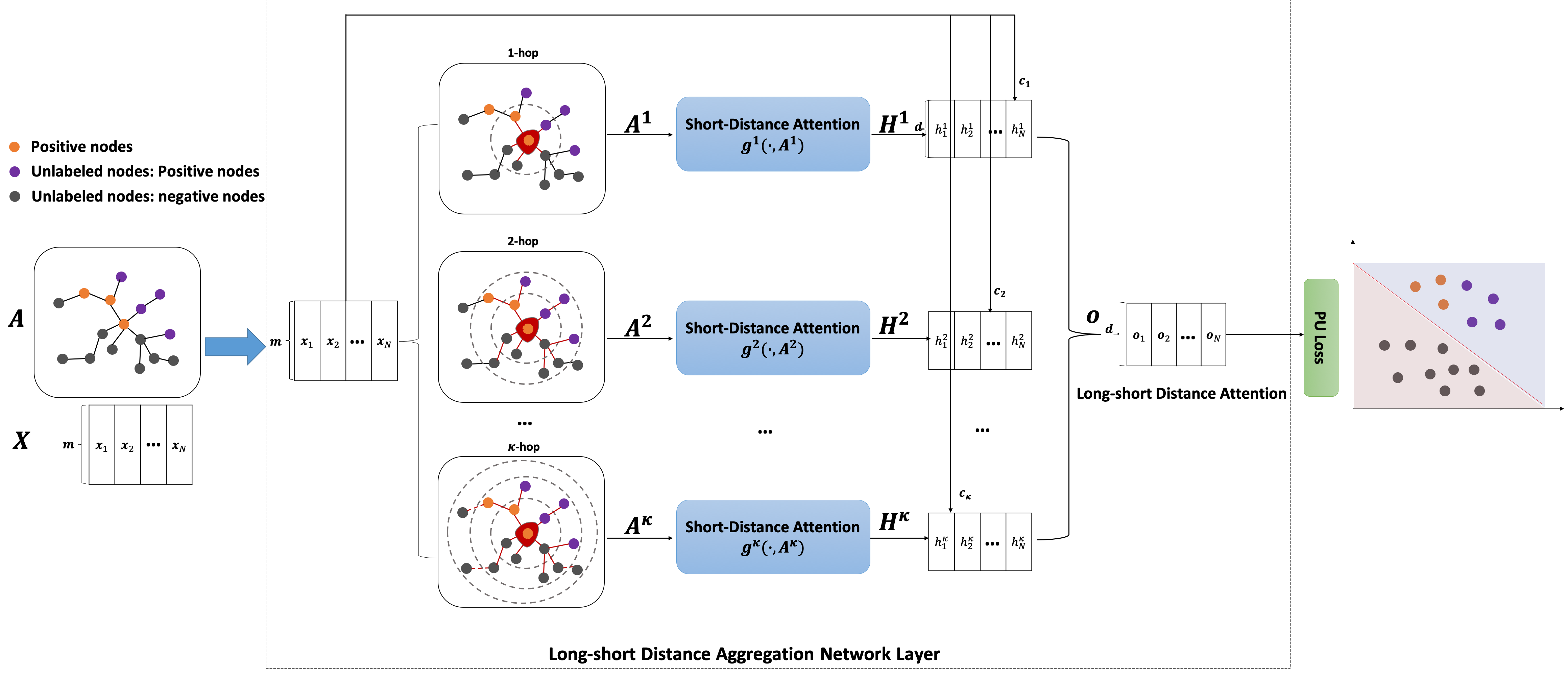
In this section, we present our proposed LSDAN algorithm for PU Graph learning. Our learning objectives are to (1) capture the long-short distance relationship between nodes, and (2) enable PU learning on a graph. We will first present our long-short distance attention network which exploits both short-distance and long-distance attention for long-short distance relationship modeling. Then we present two risk estimators for PU learning. Our framework, as shown in Figure 3, mainly consists of three components:
- •
Short-Distance Attention. For the input and an adjacent matrix , a short-distance self attention mechanism is applied to learn a representation for each node.
- •
Long-short Distance Attention. Given an input graph , we will first generate multi-hop graph representation based on adjacent matrix . The matrix captures the neighbors in the -th hop of the graph . We develop a long-distance attention approach to automatically determine the weights of different graphs .
- •
Positive Unlabeled Learning. Based on our long-short distance attention model, we develop a deep architecture for learning the graph representation of each node. Then the unbiased risk estimator and the non-negative risk estimator are used to estimate the classification loss, respectively. The loss is further back-propagated to the learning progress in an end to end learning framework.
4.1. Short-Distance vs. Long-Distance
Definition 4.1.
Short-Distance: Short-distance is defined as the distance from direct (1-hop) neighbor nodes to a target node.
The (normalized) adjacency matrix A characterizes the first-order proximity to model the direct relationship (1-hop) between vertices.
Definition 4.2.
Long-Distance: Long-distance is defined as the distances of -hop neighbors () to a target node.
In order to capture long-distance relation for each node, we propose to consider -distance (with varying ) relational information from the network for graph learning. Given an input graph , we will first generate multi-hop graph representation based on adjacent matrix . The matrix captures the neighbors in the -th hop of the graph , as shown in Figure 4. Therefore, the -distance relationship can be captured by:
| (2) |
where refers to the -hop link relation between node and . In other words, if , it means that node and have a -hop relation, or zero otherwise.

4.2. Long-short Distance Attention
In this subsection, we propose to differentiate and combine short-distance attention and long-distance attention to learn network feature representation PU learning.
4.2.1. Short-Distance Attention
Given the input denoting content matrix for all nodes where each node has dimension feature, and an adjacent matrix , a short-distance self attention mechanism is applied to learn a representation for each node, which aims to capture the node features of the whole graph with short distance by aggregating feature values within each node’s neighborhood. Specifically, the input is a set of node features, , denotes feature vector for node where denotes the number of input features of each node. The output of the short-distance attention is a new set of node features, , where and denotes the number of embedding features of each node.
| (3) |
where is a non-linear activation function, serves as a mask to only aggregate node ’s direct neighbors (short-distance neighbors) for feature learning. is weight value capturing the importance of neighbor for node . To automatically learn the parameter , a short-distance self-attention mechanism is developed.
To compute , a shared linear transformation is applied to each node through multiply a shared weight matrix in the initial step. Then an attention coefficient is computed by an attention function :
| (4) |
which measures the importance of vertex to vertex . In the most general formulation, the model allows every node to attend on every other node, dropping all structural information. We inject the graph structure into the mechanism by performing masked attention, masking out all other nodes except direct neighbors based on the adjacency matrix .
Furthermore, in order to make coefficients comparable among vertices, a softmax function is utilized to normalize attention coefficients:
| (5) |
In the experiment, the attention mechanism is instantiated with a dot product (parametrized by a weight vector ) and a LeakyReLU (Xu et al. 2015) nonlinearity. Fully expanded out, the normalized attention coefficients can be expressed as:
| (6) |
where denotes the concatenation operation of vector and .

4.2.2. Long-Distance Attention
To capture long-distance relation between nodes, we need to aggregate embedding from different range of neighborhoods to produce a unified representation. Because neighbors from different distances contribute differently to learning the representation, we propose a Long-Distance Attention scheme to capture the significance of each -hop distance graph neighbors.
Specially, for each , we will perform the self attention to learn the embedding for each node (as shown in Figure 5). In order to obtain -hop neighborhood for each node, we define a matrix to capture whether two nodes ( and are -hop neighbors).
| (7) |
By using to mask out other nodes except -hop neighbors, we can learn -hop neighbor aggregated feature embedding as follows.
| (8) |
We then use the original input , as the key of the attention mechanism, and perform attention on each graph output , , an attention coefficient is computed by an attention function : :
| (9) |
where is a shared weight matrix for long-short feature attention learning, characterizing the consistency between short-distance and long-distance aggregated features ( also enforces the input of node to have the same dimension as the hop embedding features ). In this paper, we denote as a dot-product attention function. After that, we further normalize the weight with a softmax layer.
| (10) |
After implementing the attention, final embedding output :
| (11) |
4.3. Deep Long-short Distance Aggregation Networks
The short-distance attention and long-distance attention components are integrated into a unified layer, Long-short Distance Aggregation Network Layer (LSDAN), which serves as a building block to construct a deep architecture for node classification in a single network, as shown in Figure 6. The LSDAN layers are stacked in the following way:
-
The input to the th layer is the sum of the output and the input from layer :
(12) -
A residual connection (He et al. 2016) around two sub-layers and the multi-graph information are used in different layers. The residual connection method provides the input without any transformation to the output of the th layer, which makes the th layer learn something new about the network.
-
At the first layer of the network ( = 1), let , we will not use the residual connection (i.e. ), because we need to first map a high-dimensional node representation to a low-dimensional representation.
-
At the last layer of the network ( = L), we do not use the residual connection, and map the embedding of nodes to the 2-dimensional representation for PU classification.
By this way, we can build arbitrary deep long-short distance aggregation networks to effectively learn graph representation, by leveraging the long-short distance neighboring information.

4.4. Positive and Unlabeled Graph Learning
After integrating the structure and content information via a deep long-short distance aggregation network, we will obtain the new representation in the final layer. One key question has arisen as how can we perform positive unlabelled learning from this new representation?
We first formulate the traditional binary classification problem as a risk minimization problem, and then employ two effective positive unlabeled learning methods to approximate the risk for PUGL. An unbiased risk estimator and a non-negative risk estimator are used to approximate the risk for PU learning, respectively. By minimizing the risk, our model is learned in an end-to-end manner.
4.4.1. Traditional Binary Classification
Given a set of the obtained representations , where is new feature representation of node . In the traditional binary classification, we need to learn a model , to classify each node into the predefined categories , which is the ground-truth label of the node ( denotes positive samples, denotes negative samples).
Let be a loss function, then measures the predicting loss for an output when the ground truth is . Let be a mapping function, and maps the input in the range (0,1). The traditional binary classification problem is formulated as a risk minimization problem:
| (13) |
where and are the expected loss for positive and negative samples. Here, we denote be the class-prior probability, . is assumed to known throughout the paper, and it can be estimated from positive data (Jain et al. 2016).
Therefore, for traditional binary classification problem i.e., positive and negative learning (PN Learning), we can minimize an approximated by,
| (14) |
where and . Here, and denote the number of positive/neagtive samples, respectively.
4.4.2. Unbiased Risk Estimator for PU Learning
For positive unlabeled (PU) learning, however, negative training data is unavailable. As a result, we need to estimate via Eq. (14). Here, we use a novel unbiased risk estimator to approximate (Plessis et al. 2014). Specifically, the expected loss of negative samples can be obtain by the expected loss of positive samples and the expected loss of unlabeled samples, and is defined as
| (15) |
where , and . Here, and denote the number of positive/unlabeled samples, respectively.
Therefore, for positive unlabeled (PU) learning, the risk can be approximated by,
| (16) |
4.4.3. Non-negative Risk Estimator for PU Learning
Although the unbiased risk estimator can efficiently solve the positive unlabeled learning problem. However, Eq. (16) may cause the risk value get negative, because there’s a negative sign in front of . The refers to the sample in the positive sample set which is predicted to get the expected risk value with the negative label through the model, that is: if the prediction is the negative sample, loss is 0; if the prediction is not the negative sample, loss is positive. This will cause overfitting problem for PU Learning. Motivated by Kiryo et al. 2017a, we employ a non-negative risk estimator , given as follows,
| (17) |
In our paper, we will minimize the unbiased empirical risk and non-negative empirical risk, respectively. Specifically, let be a mapping function, and we use a Sigmoid activation function to map the input o, which can be learned by our graph neural network module in Eq. (11), to the range (0,1). The Logistic Loss is used in the paper, and the loss function of each sample is defined as:
| (18) |
where and are the model predict score and the ground-truth for each sample. The expected loss/risk can be computed by the unbiased empirical risk and non-negative empirical risk via Eq. (16) and Eq. (17), respectively.
4.5. Algorithm Description
Our algorithm is illustrated in Algorithm 1. Given a graph , the goal of Positive Unlabeled Graph Learning (PUGL) is to learn the node representations and learn a binary classifier model, , to predict class labels for unlabeled nodes in .
The algorithm first obtains adjacency matrix and its power matrices from by Eq. (2) (Step 1). After that, it uses labelled node set and unlabelled node set to calculate class-prior probability from (Steps 2-4). Next, the algorithm carry out long-short distance aggregation to effectively learn node representations by leveraging the long-short distance neighboring information. The final output of node representations are denoted by (Steps 5-18). Finally, the algorithm formulates a binary classification task as a risk minimization problem, and employs two effective positive unlabeled learning methods to approximate the risk for PUGL. An unbiased risk estimator and a non-negative risk estimator are used to approximate the risk for PU learning, respectively. By minimizing the risk, the loss can be further back-propagated in our proposed model to guide the representation learning to achieve better PU graph learning results (Steps 19-23).
4.6. Time Complexity Analysis
Given a graph , the proposed Long-short Distance Aggregation Network Layer (LSDAN) consists of two parts: short-distance attentions, and long-short distance attention, where denotes the number of hops. It is worth noting that the calculation of the matrix can be done in advance, and there is no need to recalculate the matrix during the training process. The calculation of requires time complexity. The time complexity for computing each short-distance attention is , where and are the numbers of nodes and edges in the graph, respectively, and and denote the dimensions of the input feature and output feature of a single layer, respectively. The time complexity of long-short distance attention is . Therefore, the overall time complexity of the proposed Long-short Distance Aggregation Network Layer (LSDAN) is .
In real-world networks, the number of nodes and the number of edges are much larger than feature dimension , embedding size , and the the maximum hops for long-short distance aggregation , where and are more than thousands, and , , and are in hundreds maximum. In addition, we know that . Therefore, LSDAN’s complexity is asymptotically bounded by .
5. Experiments
In this section, we conduct experiments to evaluate our model against state-of-the-art algorithms on three real-world datasets. Furthermore, we also provide detailed experimental analysis to show more insights of our model.
5.1. Experiment Setting
Datasets We employ three widely used citation network datasets (Cora, Citeseer, DBLP) for node classification (Yang et al. 2015; Pan et al. 2016). The details of the experimental datasets are displayed in Table 2. The Cora dataset contains 2708 nodes, 5429 edges with 7 classes and 1433 features. The Citeseer dataset contains 3312 nodes, 4732 edges with 6 classes and 3703 features. The DBLP dataset contains 5818 nodes, 3633 edges with 4 classes and 1587 features. As these datasets have multiple classes, we select the class with the relatively large number of samples as P (positive) class, and all the other classes are regarded as N (negative) class. Specifically, for the Cora, Citeseer, and DBLP datasets, we select the class with the label is 3, 2, and 1, respectively, as P (positive) class and the remaining classes as N (negative) class. After selecting the positive class, we convert the original classification problems of each dataset into binary classification tasks.
| Dataset | Node | Edges | Classes | Features |
|---|---|---|---|---|
| Cora | 2708 | 5429 | 7 | 1433 |
| Citeseer | 3312 | 4732 | 6 | 3703 |
| DBLP | 5818 | 3633 | 4 | 1587 |
Baselines To the best of our knowledge, there is no existing study on positive unlabeled graph neural network learning. To make a fair comparison and evaluate the effectiveness of our design, we select the following baselines with necessary adaption.
We first compare our model with the classical PU learning methods, which focus on the one-step strategy and two-step strategy.
-
OC-SVM: OC-SVM (Schölkopf et al. 2014) (One-class SVM algorithm) is a classical machine learning algorithm based on support vector machine. It only uses positive examples from the node content to build a binary classifier. In our experiments, we use node features as the input of One-class SVM.
-
LINE_OC-SVM: We first use an unsupervised network embedding method (LINE (Tang et al. 2015)) to learn node representation. After that, the learned features are used as the input of One-class SVM.
-
GAE_OC-SVM: We use an unsupervised graph embedding method (Graph Auto-Encoders, GAE (Kipf and Welling 2016b)) to learn node representation by using both the adjacency matrix of nodes and the features of nodes. After that, the learned features are used as the input of One-class SVM.
-
Roc-SVM: Roc-SVM (Li and Liu 2003) uses two step strategies to build a classifier from the node content, and combines the Rocchio method and the SVM technique for PU learning algorithm. In our experiments, we use the features of nodes as the input of Roc-SVM.
-
LINE_Roc-SVM: We use an unsupervised network embedding method (LINE (Tang et al. 2015)) to learn node representation by only using the adjacency matrix of nodes. After that, the learned features are used as the input of Roc-SVM.
-
GAE_Roc-SVM: We use an unsupervised graph embedding method (Graph Auto-Encoders, GAE (Kipf and Welling 2016b)) to learn node representation by using both the adjacency matrix of nodes and the features of nodes. After that, the learned features are used as the input of Roc-SVM.
In addition the above baseline, we also compare our algorithm with different deep learning models. Note that we have integrated the unbiased risk estimator and non-negative risk estimator into the following models for PU learning.
-
FC: Full-connected network only applies node features to a multiple layer perceptron (MLP) to learn node representation without using the adjacency matrix of nodes.
-
FS: Full-connected self-attention network uses the node features with a self-attention network to obtain the representation without the adjacency matrix of nodes.
-
GCN: GCN uses the graph convolutional network (Kipf and Welling 2016a) to integrate structure and content information of nodes to learn node representation using the adjacency matrix of nodes.
-
GAT: GAT uses the graph attention nets (Velickovic et al. 2017) to exploit structure and content information of nodes to obtain node representation using the adjacency matrix of nodes. Note that, in the experiments, we only utilize one attention head.
-
GATH: GATH uses the graph attention nets (Velickovic et al. 2017) to exploit structure and content information of nodes to obtain node representation using the adjacency matrix of nodes. In addition, multi-head attention is further utilized to stabilize the learning process and encapsulate detailed information about the neighborhood.
Our method:
-
LSDAN_UPU: LSDAN_UPU employs a long-short distance aggregation network to exploit structure and content information of nodes to obtain the final graph representation, and the unbiased risk estimator is utilized for PU learning.
-
LSDAN_NNPU: LSDAN_NNPU employs a long-short distance aggregation network to exploit structure and content information of nodes to obtain the graph representation, and the non-negative risk estimator is utilized for PU learning.
Experimental Setup For fairness of comparison, we randomly split each PN dataset into positive and unlabeled set. Following Kiryo et al. 2017a, we sample (the total number of positive nodes) nodes from as negative class. Then we select nodes from as the training set, the rest positive nodes and negative nodes are used as the unlabeled set ( is the percentage of training (positive) nodes). We conduct trials of randomly splitting, and report the average F1 score as final experimental results.
All models were implemented in TensorFlow with the Adam optimizer with a learning rate of for steps. For parameter setting, we set the embedding dimension of nodes to for all methods. We choose layers for GCN-PU and GAT-PU, where the first GCN/GAT layer contains hidden units, and the second layer contains hidden units for classification. For the proposed LSDAN, the number hops is set to . The number of heads for the multi-head attention mechanism for GATH is set as 8.
5.2. Experimental Results
| %p | OC-SVM | LINE_OC-SVM | GAE_OC-SVM | Roc-SVM | LINE_Roc-SVM | GAE_Roc-SVM |
| %0.01 | 0.0230.004 | 0.0410.011 | 0.5170.099 | 0.0180.005 | 0.1770.036 | 0.3930.019 |
| %0.02 | 0.0380.011 | 0.1960.028 | 0.6140.028 | 0.0570.007 | 0.3140.024 | 0.4640.015 |
| %0.03 | 0.0540.015 | 0.3040.028 | 0.6310.024 | 0.0790.007 | 0.3810.039 | 0.4850.020 |
| %0.04 | 0.0900.009 | 0.3610.024 | 0.6460.013 | 0.1150.009 | 0.4240.026 | 0.4930.019 |
| %0.05 | 0.0890.017 | 0.4300.024 | 0.6580.011 | 0.1460.016 | 0.4460.027 | 0.5000.017 |
| %p | FC_UPU | FS_UPU | GCN_UPU | GAT_UPU | GATH_UPU | LSDAN_UPU |
| %0.01 | 0.5150.112 | 0.4560.141 | 0.3370.166 | 0.5310.083 | 0.5640.086 | 0.6470.073 |
| %0.02 | 0.5220.109 | 0.5530.051 | 0.4110.139 | 0.5780.067 | 0.6060.070 | 0.6970.067 |
| %0.03 | 0.5330.094 | 0.5780.026 | 0.4960.084 | 0.5820.038 | 0.6140.042 | 0.7100.054 |
| %0.04 | 0.5600.060 | 0.6290.017 | 0.5400.061 | 0.6450.017 | 0.6680.024 | 0.7170.051 |
| %0.05 | 0.5880.042 | 0.6810.010 | 0.5900.055 | 0.6960.019 | 0.7110.016 | 0.7380.036 |
| %p | FC_NNPU | FS_NNPU | GCN_NNPU | GAT_NNPU | GATH_NNPU | LSDAN_NNPU |
| %0.01 | 0.6840.013 | 0.6820.007 | 0.4330.258 | 0.7750.030 | 0.7770.029 | 0.7860.043 |
| %0.02 | 0.6260.054 | 0.6950.008 | 0.5640.300 | 0.7750.024 | 0.7790.022 | 0.8040.028 |
| %0.03 | 0.7100.016 | 0.7050.009 | 0.6230.259 | 0.7960.017 | 0.8030.015 | 0.8130.014 |
| %0.04 | 0.7340.013 | 0.7250.009 | 0.7210.199 | 0.8140.015 | 0.8150.009 | 0.8280.009 |
| %0.05 | 0.7430.015 | 0.7450.008 | 0.8120.011 | 0.8300.011 | 0.8320.008 | 0.8400.007 |
| %p | OC-SVM | LINE_OC-SVM | GAE_OC-SVM | Roc-SVM | LINE_Roc-SVM | GAE_Roc-SVM |
| %0.01 | 0.4450.029 | 0.3490.035 | 0.5760.033 | 0.0560.012 | 0.3550.017 | 0.5150.037 |
| %0.02 | 0.5430.009 | 0.4710.023 | 0.6240.017 | 0.1440.026 | 0.4630.029 | 0.5670.038 |
| %0.03 | 0.5800.004 | 0.5190.018 | 0.6370.012 | 0.2340.019 | 0.4990.022 | 0.5970.025 |
| %0.04 | 0.6010.006 | 0.5470.012 | 0.6430.008 | 0.3140.037 | 0.5240.027 | 0.6130.013 |
| %0.05 | 0.6110.006 | 0.5670.015 | 0.6430.007 | 0.3710.037 | 0.5450.023 | 0.6160.017 |
| %p | FC_UPU | FS_UPU | GCN_UPU | GAT_UPU | GATH_UPU | LSDAN_UPU |
| %0.01 | 0.5100.108 | 0.5230.060 | 0.3980.134 | 0.5470.033 | 0.5820.050 | 0.6870.056 |
| %0.02 | 0.5260.075 | 0.6120.022 | 0.5010.096 | 0.6550.035 | 0.6900.031 | 0.7090.067 |
| %0.03 | 0.5720.042 | 0.6450.012 | 0.5730.072 | 0.7290.023 | 0.7340.018 | 0.7400.049 |
| %0.04 | 0.6100.029 | 0.6710.010 | 0.6330.054 | 0.7490.021 | 0.7530.015 | 0.7570.035 |
| %0.05 | 0.6460.020 | 0.6930.010 | 0.6690.052 | 0.7710.013 | 0.7710.012 | 0.7770.033 |
| %p | FC_NNPU | FS_NNPU | GCN_NNPU | GAT_NNPU | GATH_NNPU | LSDAN_NNPU |
| %0.01 | 0.6500.032 | 0.6770.007 | 0.4190.128 | 0.7670.019 | 0.7750.018 | 0.8080.012 |
| %0.02 | 0.5210.092 | 0.6950.023 | 0.5990.050 | 0.8070.017 | 0.8080.014 | 0.8330.015 |
| %0.03 | 0.7100.011 | 0.7150.007 | 0.6850.032 | 0.8240.008 | 0.8250.009 | 0.8240.008 |
| %0.04 | 0.5970.046 | 0.7250.011 | 0.7340.026 | 0.8360.009 | 0.8380.009 | 0.8490.010 |
| %0.05 | 0.7410.009 | 0.7460.009 | 0.7600.024 | 0.8450.009 | 0.8450.008 | 0.8570.010 |
| %p | OC-SVM | LINE_OC-SVM | GAE_OC-SVM | Roc-SVM | LINE_Roc-SVM | GAE_Roc-SVM |
| %0.01 | 0.1110.213 | 0.1010.016 | 0.6180.046 | 0.0390.008 | 0.2290.042 | 0.4470.040 |
| %0.02 | 0.2630.004 | 0.2600.031 | 0.6980.027 | 0.0730.010 | 0.3480.032 | 0.4970.029 |
| %0.03 | 0.2930.010 | 0.3670.025 | 0.7000.019 | 0.1280.013 | 0.4110.029 | 0.5040.015 |
| %0.04 | 0.3240.014 | 0.4330.032 | 0.7010.018 | 0.1690.017 | 0.4430.030 | 0.5020.017 |
| %0.05 | 0.3580.015 | 0.4820.026 | 0.7080.014 | 0.2180.018 | 0.4650.017 | 0.5160.022 |
| %p | FC_UPU | FS_UPU | GCN_UPU | GAT_UPU | GATH_UPU | LSDAN_UPU |
| %0.01 | 0.5240.098 | 0.5030.115 | 0.4540.079 | 0.5630.080 | 0.5970.086 | 0.7460.073 |
| %0.02 | 0.5310.091 | 0.5670.056 | 0.5790.059 | 0.6930.055 | 0.7200.055 | 0.7960.050 |
| %0.03 | 0.5610.053 | 0.6230.024 | 0.6500.035 | 0.7710.022 | 0.7900.017 | 0.8240.017 |
| %0.04 | 0.5860.036 | 0.6610.019 | 0.6860.034 | 0.8080.020 | 0.8210.016 | 0.8360.018 |
| %0.05 | 0.6140.026 | 0.6860.015 | 0.7210.021 | 0.8290.016 | 0.8380.010 | 0.8430.013 |
| %p | FC_NNPU | FS_NNPU | GCN_NNPU | GAT_NNPU | GATH_NNPU | LSDAN_NNPU |
| %0.01 | 0.5420.086 | 0.6730.008 | 0.6100.248 | 0.7720.026 | 0.7820.013 | 0.8250.016 |
| %0.02 | 0.5930.039 | 0.6830.008 | 0.7710.078 | 0.8170.024 | 0.8260.022 | 0.8410.020 |
| %0.03 | 0.6410.033 | 0.6970.010 | 0.8190.041 | 0.8420.016 | 0.8480.016 | 0.8500.013 |
| %0.04 | 0.6660.028 | 0.7130.010 | 0.8420.018 | 0.8590.015 | 0.8590.010 | 0.8600.013 |
| %0.05 | 0.6910.025 | 0.7250.008 | 0.8500.012 | 0.8660.008 | 0.8660.007 | 0.8670.009 |
The results of our evaluation experiments are presented in Table 3, 4, and Table 5, Table 6, Table 7, and Table 8, Table 9, Table 10, and Table 11. From these results, we have the following observations:
- (1)
In most cases, OC-SVM and Roc-SVM are inferior to other methods. This is because the traditional shallow learning methods do not capture the underlying graph structure information. Besides, we can also find that on the DBLP data set (in Table 6, 7, and 8), when the value of %p is small, the performance of OC-SVM may be higher than that of GCN_NNPU. This may be because it is difficult for the model to learn good representation features for all nodes when there are rather few positive samples.
- (2)
Both GAE_OC-SVM and GAE_Roc-SVM outperform OC-SVM and LINE_OC-SVM, Roc-SVM and LINE_Roc-SVM, respectively. This shows the effectiveness of unsupervised graph embedding by using both the adjacency matrix of nodes and the features of node.
- (3)
GAT_UPU and GAT_NNPU outperform FC_UPU, FS_UPU, and FC_NNPU, FS_NNPU, respectively. This confirms that it is useful to take node relationships into consideration for node representation learning. Furthermore, GATH_UPU and GATH_NNPU outperform GAT_UPU and GAT_NNPU, which shows the effectiveness of introducing the multi-head attention.
- (4)
The proposed LSDAN_UPU and LSDAN_NNPU outperform GAT_UPU and GAT_NNPU which only capture short-distance neighboring information. The results show the effectiveness of our algorithm in exploiting multi-hop neighbors to capture long-short distance relationship in graph learning. Meanwhile, our model shows superior performance in positive unlabeled learning problem.
- (5)
The results also show that the proposed LSDAN_UPU and LSDAN_NNPU consistently outperform all the other baselines on all three datasets with different training ratios. It demonstrates that long-short distance aggregation network together with the unbiased and non-negative risk estimators (UPU and NNPU) can better capture data distribution and the underlying relationship among data by integrating the feature information and graph information into a unified framework.
5.3. Analysis of Different Components
As our proposed model contains two key components: the long-short distance aggregation network (LSDAN) and the positive unlabeled (PU) learning component. In this section, we compare variants of the proposed model with respect to the following aspects to demonstrate the effectiveness of the long-short distance aggregation network and the positive unlabeled (PU) learning component.
The following LSDAN variants are designed for comparison.
- •
LSDAN: A variant of LSDAN with the positive unlabeled (PU) loss being removed, and only using the cross entropy loss.
- •
LSDAN_UPU: A variant of LSDAN_UPU with the long-short distance aggregation network being removed, and only using the short-distance aggregation layer.
- •
LSDAN_NNPU: A variant of LSDAN_NNPU with the long-short distance aggregation network being removed, and only using the short-distance aggregation layer.
The ablation study results are shown in Table 12, Table 13 and Table 14.
| %p | LSDAN | LSDAN_UPU | LSDAN_UPU | LSDAN_NNPU | LSDAN_NNPU |
| %0.01 | 0.362 | 0.531 | 0.647 | 0.775 | 0.786 |
| %0.02 | 0.373 | 0.578 | 0.697 | 0.775 | 0.804 |
| %0.03 | 0.385 | 0.582 | 0.710 | 0.796 | 0.813 |
| %0.04 | 0.396 | 0.645 | 0.717 | 0.814 | 0.828 |
| %0.05 | 0.409 | 0.696 | 0.738 | 0.830 | 0.840 |
| %p | LSDAN | LSDAN_UPU | LSDAN_UPU | LSDAN_NNPU | LSDAN_NNPU |
| %0.01 | 0.431 | 0.547 | 0.687 | 0.767 | 0.808 |
| %0.02 | 0.437 | 0.655 | 0.709 | 0.807 | 0.833 |
| %0.03 | 0.441 | 0.729 | 0.740 | 0.824 | 0.824 |
| %0.04 | 0.461 | 0.749 | 0.757 | 0.836 | 0.849 |
| %0.05 | 0.472 | 0.771 | 0.777 | 0.845 | 0.857 |
| %p | LSDAN | LSDAN_UPU | LSDAN_UPU | LSDAN_NNPU | LSDAN_NNPU |
| %0.01 | 0.337 | 0.563 | 0.746 | 0.772 | 0.825 |
| %0.02 | 0.349 | 0.693 | 0.796 | 0.817 | 0.841 |
| %0.03 | 0.372 | 0.771 | 0.824 | 0.842 | 0.850 |
| %0.04 | 0.394 | 0.808 | 0.836 | 0.859 | 0.860 |
| %0.05 | 0.415 | 0.829 | 0.843 | 0.866 | 0.867 |


5.3.1. Impact of the PU loss
We compare LSDAN with LSDAN_UPU and LSDAN_NNPU to investigate the effectiveness of the positive unlabeled risk estimators employed in our paper. From the result, we find that both LSDAN_UPU and LSDAN_NNPU perform better than LSDAN, which confirms the superiority of the risk estimators for positive unlabeled learning problem.
5.3.2. Impact of long-short distance aggregation network
For fair comparisons, in the actual operation, we only employ one attention head for GAT_UPU and GAT_NNPU. In other words, LSDAN_UPU are the same as GAT_UPU, and LSDAN_NNPU are the same as GAT_NNPU. Therefor, the results of LSDAN_UPU are the the same as that of GAT_UPU, and same for LSDAN_NNPU vs. GAT_NNPU. In order to verify the effectiveness of the long-short distance aggregation network, we compare LSDAN_UPU with LSDAN_UPU, and LSDAN_NNPU with LSDAN_NNPU. From Table 12, Table 13 and Table 14, we can easily observe that LSDAN_UPU and LSDAN_NNPU perform significantly better than LSDAN_UPU and LSDAN_NNPU. This confirms that the usage of long-short distance aggregation network can learn a superior representation for nodes in graphs.
5.4. Analysis of the Learned Long-Distance Attention
We further study the learned attentions to understand why our long-distance attention mechanism helps improve the performance. Specifically, we examine which graph () attracts more attentions for the classification task. We report F1 score using only and its attention weight value learned by our LSDAN algorithm. For simplicity, we only report the results on LSDAN_NNPU which are presented in Figure 7.
The results show that the performance of the single graph () and the long-distance attention value positively correlate. For instance, on the Citeseer dataset, receives more weight as its predictive power is stronger. The results validate that our approach allows different nodes to focus on the different hops based on the adjacency matrix, to achieve better performance.
5.5. Parameter Analysis
Embedding Dimensions : We vary with , and report the results on the three datasets in Fig. 8(a). We can find that F1 scores show a clear increase from to on the Cora and DBLP, while it decreases slightly in the nd dimension in the Citeseer. When the number of embedding dimensions continuously increases, the performance starts to remain stable. This is intuitive as more embedding dimensions can encode more useful information from data.
Distance at -Hops : We also report F1 scores over different choices of with and on the three datasets in Fig. 8(b). It can be seen from Fig. 8(b) that when =4, satisfactory results have been achieved on different data sets. This confirms that the long distance relation is really important to better capture graph structure information, and multiple graphs can learn complementary local information. Simultaneously, when is greater than 4, as gets bigger and bigger, the result becomes worse, possible because some redundant information interfere the learning, and the learned -hop relational information becomes less informative for node representation learning.
Number of layers : Fig. 8(c) shows the influence of the number of layers on performance on three datasets. Here, we set , and . For the datasets considered here, best results are obtained with a - or -layer model. We can see that the setting = 2 has a significant improvement over the setting = 1 on three datasets. We observe that the performance will slightly decrease for models deeper than layers, this may overfit as the number of parameters increases with model depth.
6. Discussion
PU learning is traditionally applied to data with independent and identical distributions (i.e. non-relational data). Some earlier works have extended it to graph (relational data) databases. For example, (Zhao
et al. 2012) proposed an integrated approach
to select discriminative features for graph classification based upon positive and unlabeled graphs.
(Wu
et al. 2017) proposed a learning framework for classifying a bag of multiple graphs. Therefore, there are existing work which apply PU learning to graphs/networks, but under different learning settings.
In our problem settings, although nodes are not independent, we can assume that labels are independently provided for selected nodes (which will be marked as labeled nodes). In other words, when setting a set of nodes to be labeled, a random approach is used to select a small porting of nodes being labeled. In fact, all existing works in node classification (transductive graph learning) employ this setting. Once the labels are provided, graph neural networks here are employed to learn the new representation for each node. After each node is represented into a vector space, this task is similar to general PU learning, and then the risk estimators can be employed for PU learning.
One novelty of our approach is that we integrate the feature learning by GNNs and risk estimation into a unified and end-to-end framework. As demonstrated in our algorithm, this approach performs very well in the benchmark datasets.
In this paper, we are following common protocols in the research to set up the PU learning for graphs, with a small portion of randomly selected nodes being labeled. However, some nodes may have a higher chance being labeled, due to their linkages or connections. This is, indeed, determined by the applications and network structures. It will be a very interesting direction for future work to investigate further.
7. Conclusion
In this paper, we propose a novel long-short distance aggregation network (LSDAN) for positive unlabeled graph learning. We argue that existing algorithms largely overlook the long-distance relationship, and only exploit 1-hop neighbors to aggregate information to learn feature representation for nodes. In order to leverage long-distance relation between nodes, we propose a long-short distance aggregation network to jointly exploit the short-distance and long-short attention from different range of neighborhood to learn feature for each node. In addition, two novel risk estimators are proposed for positive unlabeled graph learning. Experiments and comparisons on three benchmark graph datasets demonstrate the effectiveness of our algorithm.
Acknowledgements.
This research is supported by the U.S. National Science Foundation (NSF) through Grant Nos. IIS-1763452, CNS-1828181, and IIS-2027339.References
- (1)
- Bruna et al. (2014) Joan Bruna, Wojciech Zaremba, Arthur Szlam, and Yann Lecun. 2014. Spectral Networks and Locally Connected Networks on Graphs. In Proc. of ICLR.
- Cao et al. (2016) Shaosheng Cao, Wei Lu, and Qiongkai Xu. 2016. Deep neural networks for learning graph representations. In Proc. of AAAI. 1145–1152.
- Chen et al. (2017) Meihao Chen, Zhuoru Lin, and Kyunghyun Cho. 2017. Graph Convolutional Networks for Classification with a Structured Label Space. In arXiv preprint arXiv:1804.08049.
- Chen et al. (2020) Yu Chen, Lingfei Wu, and Mohammed Zaki. 2020. Iterative Deep Graph Learning for Graph Neural Networks: Better and Robust Node Embeddings. Advances in Neural Information Processing Systems 33 (2020).
- Defferrard et al. (2016) Michaël Defferrard, Xavier Bresson, and Pierre Vandergheynst. 2016. Convolutional neural networks on graphs with fast localized spectral filtering. In Proc. of NIPS. 3844–3852.
- Duvenaud et al. (2015) David Duvenaud, Dougal Maclaurin, Jorge Aguilera-Iparraguirre, Rafael Gómez-Bombarelli, Timothy Hirzel, Alán Aspuru-Guzik, and Ryan P. Adams. 2015. Convolutional Networks on Graphs for Learning Molecular Fingerprints. In Proc. of NIPS. 2224–2232.
- Fout et al. (2017) Alex Fout, Jonathon Byrd, Basir Shariat, and Asa Ben-Hur. 2017. Protein interface prediction using graph convolutional networks. In Proc. of NIPS. 6530–6539.
- Gao and Ji (2019) Hongyang Gao and Shuiwang Ji. 2019. Graph u-nets. arXiv preprint arXiv:1905.05178 (2019).
- Grover and Leskovec (2016) Aditya Grover and Jure Leskovec. 2016. Node2vec: Scalable feature learning for networks. In Proc. of SIGKDD. ACM, 855–864.
- Hamilton et al. (2017a) Will Hamilton, Zhitao Ying, and Jure Leskovec. 2017a. Inductive representation learning on large graphs. In Proc. fo NIPS. 1024–1034.
- Hamilton et al. (2017b) William L. Hamilton, Zhitao Ying, and Jure Leskovec. 2017b. Inductive Representation Learning on Large Graphs. In Proc. of NIPS. 1024–1034.
- He et al. (2016) Kaiming He, Xiangyu Zhang, Shaoqing Ren, and Jian Sun. 2016. Deep residual learning for image recognition. In Proc. of CVPR. 770–778.
- Henaff et al. (2015) Mikael Henaff, Joan Bruna, and Yann Lecun. 2015. Deep Convolutional Networks on Graph-Structured Data. In arXiv preprint arXiv:1506.05163.
- Jain et al. (2016) Shantanu Jain, Martha White, and Predrag Radivojac. 2016. Estimating the class prior and posterior from noisy positives and unlabeled data. In Proc. of NIPS. 2693–2701.
- Kipf and Welling (2016a) Thomas N Kipf and Max Welling. 2016a. Semi-supervised classification with graph convolutional networks. arXiv preprint arXiv:1609.02907 (2016).
- Kipf and Welling (2016b) Thomas N Kipf and Max Welling. 2016b. Variational Graph Auto-Encoders. NIPS Workshop on Bayesian Deep Learning (2016).
- Kiryo et al. (2017a) Ryuichi Kiryo, Gang Niu, Marthinus C du Plessis, and Masashi Sugiyama. 2017a. Positive-unlabeled learning with non-negative risk estimator. In Proc. of NIPS. 1675–1685.
- Kiryo et al. (2017b) Ryuichi Kiryo, Gang Niu, Marthinus C. Du Plessis, and Masashi Sugiyama. 2017b. Positive-Unlabeled Learning with Non-Negative Risk Estimator. In Proc. of NIPS. 1674–1684.
- Li et al. (2018) Ruoyu Li, Sheng Wang, Feiyun Zhu, and Junzhou Huang. 2018. Adaptive Graph Convolutional Neural Networks. In Proc. of AAAI. 3546–3553.
- Li and Liu (2003) Xiaoli Li and Bing Liu. 2003. Learning to classify texts using positive and unlabeled data. In Proc. of IJCAI. 587–592.
- Li et al. (2016) Yujia Li, Daniel Tarlow, Marc Brockschmidt, and Richard S. Zemel. 2016. Gated Graph Sequence Neural Networks. In Proc. of ICLR.
- Liu et al. (2003) Bing Liu, Yang Dai, Xiaoli Li, Wee Sun Lee, and Philip S Yu. 2003. Building Text Classifiers Using Positive and Unlabeled Examples. In Proc. of ICDM. 179.
- Niu and Sugiyama (2015) Gang Niu and Masashi Sugiyama. 2015. Convex formulation for learning from positive and unlabeled data. In Proc. of ICML. 1386–1394.
- Pan et al. (2020) Shirui Pan, Ruiqi Hu, Sai-fu Fung, Guodong Long, Jing Jiang, and Chengqi Zhang. 2020. Learning graph embedding with adversarial training methods. IEEE Transactions on Cybernetics 50, 6 (2020), 2475–2487.
- Pan et al. (2018) Shirui Pan, Ruiqi Hu, Guodong Long, Jing Jiang, Lina Yao, and Chengqi Zhang. 2018. Adversarially regularized graph autoencoder for graph embedding. arXiv preprint arXiv:1802.04407 (2018).
- Pan et al. (2016) Shirui Pan, Jia Wu, Xingquan Zhu, Chengqi Zhang, and Yang Wang. 2016. Tri-party deep network representation. In Proc. of IJCAI. 1895–1901.
- Perozzi et al. (2014) Bryan Perozzi, Rami Al-Rfou, and Steven Skiena. 2014. Deepwalk: Online learning of social representations. In Proc. of SIGKDD. ACM, 701–710.
- Plessis et al. (2014) M. C. Du Plessis, Gang Niu, and Masashi Sugiyama. 2014. Analysis of Learning from Positive and Unlabeled Data. In Proc. of NIPS. 703–711.
- Rahimi et al. (2018) Afshin Rahimi, Trevor Cohn, and Timothy Baldwin. 2018. Semi-supervised User Geolocation via Graph Convolutional Networks. In Proc. of ACL. 2009–2019.
- Scarselli et al. (2009) Franco Scarselli, Marco Gori, Ah Chung Tsoi, Markus Hagenbuchner, and Gabriele Monfardini. 2009. The Graph Neural Network Model. IEEE Trans. Neural Networks 20, 1 (2009), 61–80.
- Schölkopf et al. (2014) Bernhard Schölkopf, John C. Platt, John Shawe-Taylor, Alex J. Smola, and Robert C. Williamson. 2014. Estimating the Support of a High-Dimensional Distribution. Neural Computation 13, 7 (2014), 1443–1471.
- Shen and Chung (2017) Xiao Shen and Fu-Lai Chung. 2017. Deep network embedding with aggregated proximity preserving. In Proceedings of the 2017 IEEE/ACM International Conference on Advances in Social Networks Analysis and Mining 2017. ACM, 40–43.
- Tang et al. (2015) Jian Tang, Meng Qu, Mingzhe Wang, Ming Zhang, Jun Yan, and Qiaozhu Mei. 2015. LINE: Large-scale Information Network Embedding. In Proc. of WWW. 1067–1077.
- Velickovic et al. (2017) Petar Velickovic, Guillem Cucurull, Arantxa Casanova, Adriana Romero, Pietro Lio, and Yoshua Bengio. 2017. Graph attention networks. arXiv preprint arXiv:1710.10903 (2017).
- Wang et al. (2019) Chun Wang, Shirui Pan, Ruiqi Hu, Guodong Long, Jing Jiang, and Chengqi Zhang. 2019. Attributed Graph Clustering: A Deep Attentional Embedding Approach. In Proc. of IJCAI. 3670–3676.
- Wang et al. (2016) Daixin Wang, Peng Cui, and Wenwu Zhu. 2016. Structural deep network embedding. In Proc. of SIGKDD. ACM, 1225–1234.
- Wu et al. (2017) Jia Wu, Shirui Pan, Xingquan Zhu, Chengqi Zhang, and Xindong Wu. 2017. Positive and Unlabeled Multi-Graph Learning. IEEE Trans. Cybernetics 47, 4 (2017), 818–829.
- Wu et al. (2019a) Man Wu, Shirui Pan, Lan Du, Ivo W. Tsang, Xingquan Zhu, and Bo Du. 2019a. Long-short Distance Aggregation Networks for Positive Unlabeled Graph Learning. In Proc. of ACM CIKM International Conference.
- Wu et al. (2020b) Man Wu, Shirui Pan, Chuan Zhou, Xiaojun Chang, and Xingquan Zhu. 2020b. Unsupervised Domain Adaptive Graph Convolutional Networks. In Proceedings of The Web Conference 2020. 1457–1467.
- Wu et al. (2019b) Man Wu, Shirui Pan, Xingquan Zhu, Chuan Zhou, and Lei Pan. 2019b. Domain-adversarial graph neural networks for text classification. In 2019 IEEE International Conference on Data Mining (ICDM). IEEE, 648–657.
- Wu et al. (2020a) Zonghan Wu, Shirui Pan, Fengwen Chen, Guodong Long, Chengqi Zhang, and Philip S Yu. 2020a. A comprehensive survey on graph neural networks. IEEE Transactions on Neural Networks and Learning Systems (2020).
- Xu et al. (2015) Bing Xu, Naiyan Wang, Tianqi Chen, and Mu Li. 2015. Empirical evaluation of rectified activations in convolutional network. arXiv preprint arXiv:1505.00853 (2015).
- Xu et al. (2018a) Keyulu Xu, Weihua Hu, Jure Leskovec, and Stefanie Jegelka. 2018a. How powerful are graph neural networks? arXiv preprint arXiv:1810.00826 (2018).
- Xu et al. (2018b) Linchuan Xu, Xiaokai Wei, Jiannong Cao, and Philip S Yu. 2018b. On exploring semantic meanings of links for embedding social networks. In Proceedings of the 2018 World Wide Web Conference. International World Wide Web Conferences Steering Committee, 479–488.
- Yang et al. (2015) Cheng Yang, Zhiyuan Liu, Deli Zhao, Maosong Sun, and Edward Y Chang. 2015. Network representation learning with rich text information.. In Proc. of IJCAI. 2111–2117.
- You et al. (2018) Jiaxuan You, Bowen Liu, Zhitao Ying, Vijay S. Pande, and Jure Leskovec. 2018. Graph Convolutional Policy Network for Goal-Directed Molecular Graph Generation. In Proc. of NIPS. 6412–6422.
- You et al. (2020) Jiaxuan You, Zhitao Ying, and Jure Leskovec. 2020. Design space for graph neural networks. Advances in Neural Information Processing Systems 33 (2020).
- Yun et al. (2019) Seongjun Yun, Minbyul Jeong, Raehyun Kim, Jaewoo Kang, and Hyunwoo J Kim. 2019. Graph transformer networks. In Advances in Neural Information Processing Systems. 11983–11993.
- Zhang et al. (2018a) Jiani Zhang, Xingjian Shi, Junyuan Xie, Hao Ma, Irwin King, and Dit-Yan Yeung. 2018a. GaAN: Gated Attention Networks for Learning on Large and Spatiotemporal Graphs. In Proc. of UAI. 339–349.
- Zhang et al. (2018b) Zhen Zhang, Hongxia Yang, Jiajun Bu, Sheng Zhou, Pinggang Yu, Jianwei Zhang, Martin Ester, and Can Wang. 2018b. ANRL: Attributed Network Representation Learning via Deep Neural Networks.. In Proc. of IJCAI, Vol. 18. 3155–3161.
- Zhao et al. (2012) Yuchen Zhao, Xiangnan Kong, and Philip S Yu. 2012. Positive and Unlabeled Learning for Graph Classification. In Proc. of ICDM. 962–971.