An auditory cortex model for sound processing

Human capacity for speech recognition with reduced intelligibility has mostly been studied from a phenomenological and descriptive point of view (see [18] for a review on noise in speech, as well as a wide range of situations in [2, 17]). What is lacking is a proper mathematical model informing us on how the human auditory system is able to reconstruct a degraded speech sound. The aim of this study is to provide a neuro-geometric model for sound reconstruction based on the description of the functional architecture of the auditory cortex.

Knowledge on the functional architecture of the auditory cortex and the principles of auditory perception are limited. For that reason, we turn to recent advances in the mathematical modeling of the functional architecture of the primary visual cortex and the processing of visual inputs [21, 12, 8] (which recently yield very successful applications to image processing [14, 23, 10] ) to extrapolate a model of the auditory cortex. This idea is not new: neuroscientists take models of V1 as a starting point for understanding the auditory system (see, e.g., [19]). Indeed, biological similarities between the structure of the primary visual cortex (V1) and the primary auditory cortex (A1) are well-known to exist. V1 and A1 share a “topographic” organization, a general principle determining how visual and auditory inputs are mapped to those neurons responsible for their processing [25]. Furthermore, the existence of receptive fields of neurons in V1 and A1 that allow for a subdivision of neurons in “simple” and “complex” cells supports the idea of a “common canonical processing algorithm within cortical columns” [26].

The neuro-geometric model of V1 finds its roots in the experimental results of Hubel and Wiesel [15]. This gave rise to the so-called sub-Riemannian model of V1 in [22, 12, 8, 23]. The main idea behind this model is that an image, seen as a function $f:\mathbb{R}^{2}\to\mathbb{R}_{+}$ representing the grey level, is lifted to a distribution on $\mathbb{R}^{2}\times P^{1}$, the bundle of directions of the plane. Here, $P^{1}$ is the projective line, i.e., $P^{1}=\mathbb{R}/\pi\mathbb{Z}$. More precisely, the lift is given by $Lf(x,y,\theta)=\delta_{Sf}(x,y,\theta)f(x,y)$ where $\delta_{S_{f}}$ is the Dirac mass supported on the set $S_{f}\subset\mathbb{R}^{2}\times P^{1}$ of points $(x,y,\theta)$ such that $\theta$ is the direction of the tangent line to $f$ at $(x,y)$.

When $f$ is corrupted (i.e. when $f$ is not defined in some region of the plane), the reconstruction is obtained by applying a deeply anisotropic diffusion mimicking the flow of information along the horizontal and vertical connections of V1, with initial condition $L_{f}$. This diffusion is known as the sub-Riemannian diffusion in $\mathbb{R}^{2}\times P^{1}$, cf. [1]. One of the main features of this diffusion is that it is invariant by rototranslation of the plane, a feature that will not be possible to translate to the case of sounds, due to the special role of the time variable.

The V1-inspired pipeline is then the following: first a lift of the input signal to an adequate contact space, then a processing of the lifted signal according to sub-Riemannian diffusions, then projection of the output to the signal space.

The sensory input reaching A1 comes directly from the cochlea. The sensors are tonotopically organized (in a frequency-specific fashion), with cells close to the base of the ganglion being more sensitive to low-frequency sounds and cells near the apex more sensitive to high-frequency sounds, see Figure 1. This implies that sound is transmitted to the primary auditory cortex A1 in the form of a ‘spectrogram’: when a sound $s:[0,T]\to\mathbb{R}$ is heard, A1 is fed with its time-frequency representation $S:[0,T]\times\mathbb{R}\to\mathbb{C}$. If $s\in L^{2}(\mathbb{R}^{2})$, as given by the short-time Fourier transform of $s$, that is

Here, $W:\mathbb{R}\to[0,1]$ is a compactly supported (smooth) window, so that $S\in L^{2}(\mathbb{R}^{2})$. The function $S$ depends on two variables: the first one is time, that here we indicate with the letter $\tau$, and the second one is frequency, denoted by $\omega$.

Since $S$ is complex-valued, it can be thought as the collection of two black-and-white images: $|S|$ and $\arg S$. Roughly speaking, $|S(\tau,\omega)|$ represents the strength of the presence of the frequency $\omega$ at time $\tau$. In the following, we call $S$ the sound image. The V1-inspired approach is then to apply image perception models on $|S|$. However, in this case time plays a special role: the whole sound image does not reach the auditory cortex simultaneously, but sequentially, and invariance by image rotations is lost. As a consequence, different symmetries have to be taken into account and a different model for both the lift and the processing in the contact space are required.

The discretization of the time and frequency domains is determined by the sampling rate of the original signal and the window size chosen in the STFT procedure. That is, by the Nyquist-Shannon sampling theorem, for a temporal sampling rate $\delta t$ and a window size of $T_{w}$, we consider the frequencies $\omega$ such that $|\omega|<1/(2\delta t)$, with a finest discretization rate of $1/(2T_{w})$. Observe, in particular, that the frequency domain is bounded. Nevertheless, the chirpiness $\nu$ defined as $\nu\partial_{\omega}\left\lvert S\right\rvert(\tau,\omega)+\partial_{\tau}\left\lvert S\right\rvert(\tau,\omega)=0$ is unbounded and, since generically there exists points such that $\partial_{\omega}|S|(\tau_{0},\omega_{0})=0$, it stretches over the entire real line.

To overcome this problem, a natural strategy is to model the chirpiness values as a random variable, and considering only chirpinesses falling inside the confidence interval $I_{p}$ for some reasonable $p$-value (e.g., $p=0.95$). A reasonable assumption for the distribution of $X$ is that it follows a Cauchy distribution $\mathrm{Cauchy}(x_{0},\gamma)$. Indeed, this corresponds to assuming that $\partial_{\omega}|S|$ and $\partial_{\tau}|S|$ are normal (and independent) distributions [20]. As it is customary, we chose as estimator for the location parameter $x_{0}$ the median of $X$ and for the scale parameter $\gamma$ half the interquartile distance.

Although statistical tests on a library of real-world speech signals ^††footnotemark: rejected the assumption that $X\sim\mathrm{Cauchy}(x_{0},\gamma)$, the fit is quite good according to the Kolmogorov-Smirnov statistic $D_{n}=\sup_{x}\left\lvert F_{n}(x)-F_{X}(x)\right\rvert$. Here, $F_{X}$ is the cumulative distribution function of $X$ and $F_{n}$ is the empirical distribution function evaluated over the chirpiness values.

For simple experiments on synthetic sounds, highligting the characteristics of the proposed algorithm, we refer to [9].

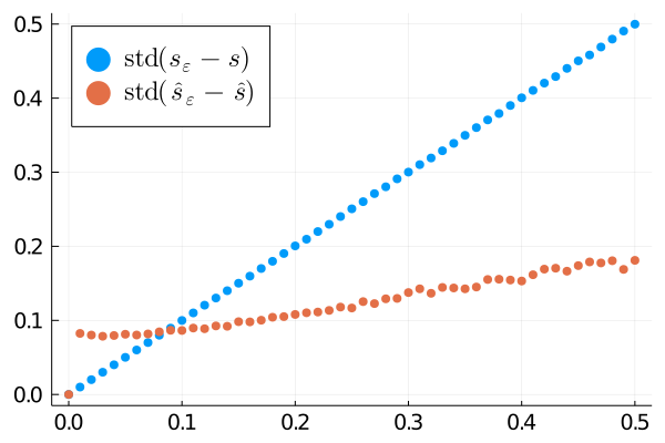
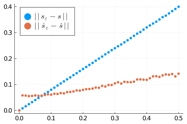
In Figure 4 we present the results of the algorithm applied to a denoising task. Namely, given a sound signal $s$, we let $s_{\varepsilon}=s+g_{\varepsilon}$, where $g_{\varepsilon}\sim\mathcal{N}(0,\varepsilon)$ is a gaussian random variable. We then apply the proposed sound processing algorithm to obtain $\widehat{s_{\varepsilon}}$. As a reconstruction metric we present both the norm $\left\lVert\cdot\right\rVert$ where for a real signal $s$, $\left\lVert s\right\rVert=\left\lVert s\right\rVert_{1}/\dim(s)$ with $\left\lVert\cdot\right\rVert_{1}$ as the $L_{1}$ norm and the standard deviation $\mathrm{std}(\widehat{s_{\varepsilon}}-\widehat{s})$. We observe that according to both metrics the algorithm indeed improves the signal.

References

- [1] Agrachev, A., Barilari, D., Boscain, U.: A Comprehensive Introduction to Sub-Riemannian Geometry. Cambridge Studies in Advanced Mathematics, Cambridge University Press (2019)
- [2] Assmann, P., Summerfield, Q.: The Perception of Speech Under Adverse Conditions, pp. 231–308. Springer New York, New York, NY (2004)
- [3] Barilari, D., Boarotto, F.: Kolmogorov-fokker-planck operators in dimension two: heat kernel and curvature (2017)
- [4] Bertalmío, M., Calatroni, L., Franceschi, V., Franceschiello, B., Gomez Villa, A., Prandi, D.: Visual illusions via neural dynamics: Wilson-cowan-type models and the efficient representation principle. Journal of Neurophysiology (2020)
- [5] Bertalmío, M., Calatroni, L., Franceschi, V., Franceschiello, B., Prandi, D.: A cortical-inspired model for orientation-dependent contrast perception: A link with wilson-Cowan equations. In: Scale Space and Variational Methods in Computer Vision. Springer International Publishing, Cham (2019)
- [6] Bertalmìo, M., Calatroni, L., Franceschi, V., Franceschiello, B., Prand i, D.: Cortical-inspired Wilson-Cowan-type equations for orientation-dependent contrast perception modelling. J. Math. Imaging Vision (2020)
- [7] Boscain, U., Chertovskih, R., Gauthier, J.P., Remizov, A.: Hypoelliptic diffusion and human vision: a semi-discrete new twist on the petitot theory. SIAM J. Imaging Sci. 7(2), 669–695 (2014)
- [8] Boscain, U., Duplaix, J., Gauthier, J.P., Rossi, F.: Anthropomorphic image reconstruction via hypoelliptic diffusion (2010)
- [9] Boscain, U., Prandi, D., Sacchelli, L., Turco, G.: A bio-inspired geometric model for sound reconstruction. The Journal of Mathematical Neuroscience 11(1), 2 (2021)
- [10] Boscain, U.V., Chertovskih, R., Gauthier, J.P., Prandi, D., Remizov, A.: Highly corrupted image inpainting through hypoelliptic diffusion. J. Math. Imaging Vision 60(8), 1231–1245 (2018)
- [11] Bressloff, P.C., Cowan, J.D., Golubitsky, M., Thomas, P.J., Wiener, M.C.: Geometric visual hallucinations, Euclidean symmetry and the functional architecture of striate cortex. Philosophical Transactions of the Royal Society of London B: Biological Sciences 356(1407), 299–330 (2001)
- [12] Citti, G., Sarti, a.: A Cortical Based Model of Perceptual Completion in the Roto-Translation Space. J. Math. Imaging Vis. 24(3), 307–326 (feb 2006)
- [13] Ermentrout, G.B., Cowan, J.D.: A mathematical theory of visual hallucination patterns. Biological cybernetics 34, 137–150 (1979)
- [14] Franken, E., Duits, R.: Crossing-Preserving Coherence-Enhancing Diffusion on Invertible Orientation Scores. International Journal of Computer Vision 85(3), 253–278 (2009)
- [15] Hubel, D.H., Wiesel, T.N.: Receptive fields of single neurons in the cat’s striate cortex. The Journal of Physiology 148(3), 574–591 (1959)
- [16] Loebel, A., Nelken, I., Tsodyks, M.: Processing of Sounds by Population Spikes in a Model of Primary Auditory Cortex. Frontiers in Neuroscience 1(1), 197–209 (2007)
- [17] Luce, P.A., McLennan, C.T.: Spoken Word Recognition: The Challenge of Variation, chap. 24, pp. 590–609. ”John Wiley & Sons, Ltd” (2008)
- [18] Mattys, S., Davis, M., Bradlow, A., Scott, S.: Speech recognition in adverse conditions: A review. Language, Cognition and Neuroscience 27(7-8), 953–978 (9 2012)
- [19] Nelken, I., Calford, M.B.: Processing Strategies in Auditory Cortex: Comparison with Other Sensory Modalities, pp. 643–656. Springer US, Boston, MA (2011)
- [20] Papoulis, A.: Probability, Random Variables and Stochastic Processes, p. 138. McGraw-Hill Companies, 3rd edn. (1991)
- [21] Petitot, J., Tondut, Y.: Vers une neurogéométrie. fibrations corticales, structures de contact et contours subjectifs modaux. Mathématiques et Sciences humaines 145, 5–101 (1999)
- [22] Petitot, J., Tondut, Y.: Vers une Neurogéométrie. Fibrations corticales, structures de contact et contours subjectifs modaux pp. 1–96 (1999)
- [23] Prandi, D., Gauthier, J.P.: A semidiscrete version of the Citti-Petitot-Sarti model as a plausible model for anthropomorphic image reconstruction and pattern recognition. SpringerBriefs in Mathematics, Springer International Publishing, Cham (2017)
- [24] Rankin, J., Sussman, E., Rinzel, J.: Neuromechanistic Model of Auditory Bistability. PLoS Computational Biology 11(11), e1004555 (nov 2015)
- [25] Rauschecker, J.P.: Auditory and visual cortex of primates: a comparison of two sensory systems. The European journal of neuroscience 41(5), 579–585 (03 2015)
- [26] Tian, B., Kuśmierek, P., Rauschecker, J.P.: Analogues of simple and complex cells in rhesus monkey auditory cortex. Proceedings of the National Academy of Sciences 110(19), 7892–7897 (2013)
- [27] Wilson, H.R., Cowan, J.D.: Excitatory and inhibitory interactions in localized populations of model neurons. Biophysical journal 12(1), 1–24 (jan 1972)
- [28] Zulfiqar, I., Moerel, M., Formisano, E.: Spectro-Temporal Processing in a Two-Stream Computational Model of Auditory Cortex. Frontiers in Computational Neuroscience 13, 95 (jan 2020)