A method of immersed layers on Cartesian grids,
with application to incompressible flows

Let us suppose that $\varphi$ is a piecewise twice-differentiable scalar field in each region separated by $\chi=0$, vanishing at infinity. We can obviously define the masked form $\overline{\varphi}$ in the same manner as (1). The gradient of $\overline{\varphi}$ follows from (2). And furthermore, the divergence of the gradient follows from (114). From these, it is easy to show from the identities in A that

where, using our notation (110), we have defined a masked form of the Laplacian operation,

Suppose that each $\varphi^{\pm}$ individually satisfies a Poisson equation in its respective region:

where $q^{+}$ and $q^{-}$ are integrable source functions. Then $\overline{\nabla^{2}\varphi}=\overline{q}$, and equation (4) with this substitution represents a generalized form of the Poisson equation for the function $\overline{\varphi}$. The Laplacian of the masked form $\overline{\varphi}$ explicitly introduces jumps on the surface $\chi=0$ in both the function itself as well as its normal derivative into an augmented form of the source function. In fact, these are familiar as single- and double-layer potentials, respectively, with corresponding strengths $\bm{n}\cdot(\nabla\varphi^{+}-\nabla\varphi^{-})$ and $\varphi^{+}-\varphi^{-}$. We can formally solve the generalized Poisson equation (4) with the help of Green’s function of the (negative of the) Laplacian, $G$, defined by

In A.3 we develop the Green’s function solution to equation (4),

By identity (86), the second and third integrals are equivalent to surface integrals on $\chi=0$, expressing the influence of the jumps in the normal derivative of $\varphi$ and of $\varphi$ itself on this surface, corresponding to standard single- and double-layer potentials, respectively. Unsurprisingly, the solution (2.1) is equivalent to the Green’s function solution of the usual Poisson equation (obtained from integrals over each region).

The Green’s function form (2.1) serves as a starting point for solving problems with known boundary data [26]. For example, suppose that we seek the solution for discontinuous Dirichlet boundary conditions, $\varphi^{+}=\varphi^{+}_{b}$ and $\varphi^{-}=\varphi^{-}_{b}$ on the surface $\chi=0$. We would substitute the jump in these known values into the double-layer potential, and seek the unknown jump in normal derivatives in the single-layer potential by setting the full expression (2.1) equal to the known value of $\overline{\varphi}$ on the surface, $(\varphi^{+}_{b}+\varphi^{-}_{b})/2$. However, for our later use in the discrete problem, it is helpful to express this procedure in a saddle-point form. We denote the unknown strength distribution of the single-layer potential by $\sigma=\bm{n}\cdot(\nabla\varphi^{+}-\nabla\varphi^{-})$. Then, we can write the problem for $\overline{\varphi}$ and $\sigma$ as

which emphasizes the role of the single-layer strength $\sigma$ as a Lagrange multiplier for enforcing the Dirichlet conditions on the masked function $\overline{\varphi}$. This form demonstrates the roles of the companion functions, $\delta(\chi)$ and $\delta^{T}(\chi)$ for, respectively, immersing surface data into the full space and for restricting a full-space function onto the surface. We will pose the problem in this form later in the discrete context, where we will also show that these functions become the familiar regularization and interpolation operators—transposes of one another—in immersed boundary methods.

An important special case of (4) and its solution (2.1) emerges when we take $\varphi^{+}=0$ and $\varphi^{-}=1$, both of which are trivial solutions of Laplace’s equations in their respective regions. The masked function corresponding to these is simply $\overline{\varphi}=H(-\chi)$, and equation (4) reduces to

This equation, which can be interpreted as a governing equation for the interior masking function $H(-\chi)$, will serve a crucial role in our development of discrete masking functions later in the paper. The solution (2.1) reduces to

In this manner, the interior mask is effectively generated by a double-layer potential of strength $-1$ on the level set $\chi=0$. The exterior mask $H(\chi)$ follows immediately from the fact that $H(\chi)=1-H(-\chi)$. We will develop discrete analogs of these expressions in Section B.

We note, in passing, that one is tempted to use (2.1) to form an expression similar to (11) for this exterior mask. However, we cannot simply set $\varphi^{+}=1$ and $\varphi^{-}=0$, since we have assumed that $\varphi^{+}$ vanishes at infinity. Indeed, we cannot obtain the uniform value of $1$—a homogeneous solution of the Poisson equation—by means of the Green’s theorem (2.1).

Let us now consider a generic inhomogeneous convection-diffusion equation for a scalar quantity $\varphi$

where $\bm{v}$ is the velocity of the fluid, $q$ is a volumetric forcing term, and the flux vector $\bm{Q}$ has the typical form $\bm{Q}=-\kappa\nabla\varphi$. We will assume that this equation governs both the interior and exterior regions. For simplicity, we will also assume that the scalar diffusion coefficient $\kappa$ is uniform and identical in both regions, though we are not restricted to do so. We wish to write this equation in masked form, with each of the quantities in the equation replaced by a masked version. Using the results obtained in A.2, it is straightforward to show that this form is

where we have defined the surface force function, $\sigma$, as

where $\dot{\bm{X}}$ denotes the local velocity of the surface $\chi=0$. The function $\sigma$ represents the net diffusive plus convective flux through the surface. Using the form of the flux vector and equation (2), we can write the masked version of this flux vector as

and the final form of the masked convection-diffusion equation is thus

When Dirichlet conditions $\varphi^{\pm}=\varphi^{\pm}_{b}$ are imposed on the interface $\chi=0$, the final term in (16) becomes a known forcing (similar to the double layer in the Poisson equation) and the surface force function $\sigma$ serves, as in the case of the Poisson equation, as a Lagrange multiplier for the constraint $\delta^{T}(\chi)\overline{\varphi}=\frac{1}{2}(\varphi^{+}_{b}+\varphi^{-}_{b})$. Once $\sigma$ is found as part of the solution, it can be interpreted physically via (14).

In this section, we formulate the Navier–Stokes equations for incompressible flow in a masked form appropriate for all of $\mathbb{R}^{d}$, when these equations govern the regions both interior and exterior to the interface $\chi=0$, i.e.,

where $\bm{I}$ is the identity tensor in $\mathbb{R}^{d}$. We will assume that the viscosity $\mu$ is uniform and identical in each region. Much of the work we performed in developing the convection-diffusion equation (16) is immediately useful here, with some minor adaptations needed to accommodate the tensor form of $\bm{S}$. Here, the equations become

The right-hand side of the continuity equation represents a distributed set of sources that correct for a possible jump in normal velocity on the interface. The surface force function $\bm{\sigma}$ is the sum of surface tractions on either side, plus the jump in momentum fluxes through the surface,

and we have defined the symmetric viscous surface tensor $\bm{\Sigma}$ as

This surface tensor introduces the interface’s velocity jump into the rate of deformation tensor in the Newtonian fluid model. As in the previous model equations, the surface force function $\bm{\sigma}$ can serve as a Lagrange multiplier for enforcing the Dirichlet (no-slip) boundary condition for $\overline{\bm{v}}$ on the surface $\chi=0$,

Thus far, these equations are quite generally applicable to several scenarios. Let us suppose our goal is to solve for a flow exterior to a closed body whose bounding surface is defined by the level set $\chi=0$ and moves with local velocity $\dot{\bm{X}}=\bm{v}_{b}$. Thus, the boundary condition we seek to enforce on this surface is $\bm{v}_{b}^{+}=\bm{v}_{b}$. We will discuss two possible approaches to using equations (18) to solve this flow, which differ in the manner in which we set a condition on $\bm{v}_{b}^{-}$ in the superfluous interior region.

In the first approach, we also set $\bm{v}_{b}^{-}=\bm{v}_{b}$, and the governing equations (18) reduce to

These equations are of the form used in the immersed boundary method [23] and the immersed boundary projection method [27]. It is important to observe that the surface force function $\bm{\sigma}$ is equal to $(\bm{S}^{+}-\bm{S}^{-})\cdot\bm{n}$, the sum of the surface tractions exerted from either side, in this approach. Thus, if one desires the exterior traction $\bm{S}^{+}\cdot\bm{n}$, it is not possible to obtain it from $\bm{\sigma}$ without some independent knowledge of the flow generated in the interior region. Such knowledge is available in special cases: a stationary surface, in which case $\bm{v}^{-}$ is identically zero throughout the interior region, so $\bm{S}^{-}$ itself is zero; and uniform $\bm{v}_{b}$—i.e., rigid-body translation—so that $\bm{v}^{-}=\bm{v}_{b}$ is the solution at all times in the interior. In this latter case, the integral of the interior traction $\bm{S}^{-}\cdot\bm{n}$ is equal to the rate of change of rigid-body momentum in the interior [31], and its local value could be determined by considering the distributed force required to ensure rigid-body motion. For cases of rigid-body rotation or deforming body motion, however, a non-trivial flow is generated in the interior by the imposed boundary condition.

In this first approach, our difficulty arises from keeping the exterior and interior regions coupled to one another via their shared boundary condition. Thus, in the second approach, we isolate the exterior region from the interior by explicitly setting the interior boundary condition to zero, $\bm{v}_{b}^{-}=0$, ensuring that the velocity and stress throughout this region is also zero. This results in the following set of equations for $\overline{\bm{v}}$, slightly more complicated than in the first approach:

Now, the surface traction can be easily found from the Lagrange multiplier $\bm{\sigma}$ and the known momentum flux by a slight re-arrangement of (19):

The overall force and moment on any body can easily be obtained by integrating. A similar approach can be used, simply by setting $\bm{v}_{b}^{+}=0$ and $\bm{v}_{b}^{-}=\bm{v}_{b}$, if the desire is to simulate an interior flow and preserve quiescent flow in the exterior region.

It is useful to express the incompressible flow equations for $\overline{\bm{v}}$ in vorticity form. We will use the general set of equations (18) as a starting point, and either of the approaches we outlined in the previous section can be expressed in a vorticity form with the equations we establish here. We first note that, from (115), the curl of the masked velocity has the form

The first term on the right-hand side is the masked vorticity, bounded everywhere but possibly discontinuous on the interface. The second term represents the strength of a vortex sheet, associated with the jump in velocity across the interface. For shorthand, we have denoted the overall curl of velocity, including the singular part associated with the vortex sheet, by $\overline{\bm{\omega}}_{\mathrm{t}}$. We will refer to this as the augmented vorticity field.

The vorticity form of Navier-Stokes arises, as usual, by taking the curl of these equations. It follows easily that

in which $\bm{\sigma}$ remains the Lagrange multiplier for the boundary condition on the velocity, the no-slip condition (21). It should be noted that this set of equations holds for the augmented vorticity field, $\overline{\bm{\omega}}_{\mathrm{t}}$, including the vortex sheet associated with the jump in interface velocities.

To recover the velocity from the vorticity field, we rely as usual on a vector potential, $\overline{\bm{\psi}}$ (streamfunction in two dimensions), assumed to have zero divergence. The masked velocity field cannot be written entirely as the curl of a vector potential because of the jump in normal velocities on the right-hand side of the continuity equation; this calls for an additional scalar potential field, $\overline{\varphi}$. We also include a uniform flow, if present, and write the overall masked velocity field using the Helmholtz decomposition as

It should be noted that, in obtaining this masked form of the decomposition, we have required that the exterior and interior values $\bm{\psi}^{\pm}$ and $\varphi^{\pm}$ each match across the interface to eliminate singular terms in these potentials and ensure that the velocity field is non-singular. By taking the curl and divergence, respectively, of (27), we obtain Poisson equations for each of the potentials,

The only boundary conditions on $\overline{\bm{\psi}}$ and $\overline{\varphi}$ are that they should vanish at infinity. Each of them is readily solved by the Green’s function treatment described in Section 2.1. The velocity in (27) is constituted from the solutions. Thus, with these equations and (26), we obtain a vorticity form of Navier–Stokes in which we can apply a specific set of conditions on the interface, as in the velocity–pressure form discussed in the previous section.

Our starting point for these will be to write the discrete analog of equation (3), but for the interior masking function $H(-\chi)$, letting $\mathsf{H}_{\mathcal{C}}^{-}$ denote the discrete form of this function on the space of cell centers, $\mathcal{C}$. The discrete equation we propose is

The grouping on the right-hand side, $\mathsf{R}_{\mathcal{F}}\bm{\mathsfit{n}}$, which regularizes the surface normal vectors onto the cell faces on the grid, is a discrete version of $\delta(\chi)\bm{n}$ and important in the rest of this paper. Equation (30) does not quite give us a means of finding $\mathsf{H}_{\mathcal{C}}^{-}$, but if we take the discrete divergence of this equation, we get

where $\mathsf{D}$ is the discrete divergence. Thus, the masking operator is generated from source data comprising the divergence of the regularized normals of the discretized surface. The lattice Green’s function on the cell centers and its associated inverse Laplacian $\mathsf{L}^{-1}_{\mathcal{C}}$ allow us to immediately write the solution of (31):

Thus, we have formed the interior masking operator $\mathsf{H}_{\mathcal{C}}^{-}$ on the grid for a particular closed shape (or set of shapes), represented discretely by a set of immersed points and their associated areas and normals. An example of this masking operator, constructed for several shapes, is shown in Figure 2. The exterior masking operator is easily obtained from the interior one, $\mathsf{H}_{\mathcal{C}}^{+}=\mathsf{1}-\mathsf{H}_{\mathcal{C}}^{-}$. The masking operators for vector-valued data, $\mathsf{H}_{\mathcal{F}}^{\pm}\in\mathcal{F}$, are defined by interpolating the cell-centered functions:

The discrete Heaviside function defined in equation (32) and the associated masking identities that will be developed in this section form the foundations of the present framework. It must be emphasized that, although we apply them using finite difference methods on a staggered Cartesian grid, these foundational equations are independent of the type of grid (structured or unstructured) or numerical method (finite difference, finite volume). Nevertheless, we now make use of some of the relationships available on a staggered grid to establish some helpful discrete identities for our current implementation. It can be readily shown that the divergence and Laplacian operations commute with one another on a staggered grid,

If we right multiply by $\mathsf{L}^{-1}_{\mathcal{F}}$ and left multiply by $\mathsf{L}^{-1}_{\mathcal{C}}$, then this commutativity extends to the inverses, as well:

Thus, the interior masking function in (32) can equivalently be written as

This form is the discrete analog of (11). Their difference in sign is due to the fact that the inverse of the discrete Laplacian is constituted by the negative of the lattice Green’s function.

With the definitions presented thus far in this section, we can immediately obtain three crucial identities. The first arises when we apply the discrete gradient $\mathsf{G}$ to the masked vector

where $\mathsf{f}^{\pm}\in\mathcal{C}$. Using the first of a series of discrete product rules (128) and the defining equation (30) for the masking function, we get the discrete version of equation (2) expressing the gradient of a masked scalar-valued grid vector:

where ${}^{\mathcal{F}}\mathsf{I}_{\mathcal{C}}$ is the interpolation operator from $\mathcal{F}$ to $\mathcal{C}$ and, for convenience, we have defined $\overline{\mathsf{G}\mathsf{f}}$ to denote the masked form of the gradient,

The second identity arises by applying the discrete divergence $\mathsf{D}$ to the masked function

where $\mathsf{u}^{\pm}\in\mathcal{F}$. Applying the second discrete product rule (129) and the definition (30), we now get the discrete version of equation (114) expressing the divergence of a masked vector-valued grid vector:

where

Though we do not present them, one can also generate similar identities for the discrete curl and gradient of vector-valued data and for the divergence of tensor-valued data, each of which also arises in the applications to follow.

Finally, by combining the identities (38) and (42), it is straightforward to show that the discrete Laplacian applied to the masked vector (37) is

where the masked Laplacian is defined as

Equation (43) is the discrete equivalent of equation (4).

Identities (38), (42), and (43), analogous to their continuous counterparts, incorporate the jumps in field quantities across an interface into the discrete calculus operations on these field data. In particular, by simple comparison between (43) and the continuous equation (4), the second term on the right-hand side of (43) resembles a discrete form of a single layer and the third term a discrete double layer. However, they use the grid itself to attach these jumps to the interface, so they are not in a form that readily allows us to introduce known data or prescribed conditions on the interface into the discrete operators. For such purposes, we would expect the discrete interface terms to each contain an element from the immersed point space $\mathcal{S}^{N}$ to describe the jump. Thus, we will define scalar-valued quantities on the sets of immersed points $\mathsfit{s},\mathsfit{d}\in\mathcal{S}^{N}$ as follows:

for $\mathsf{u}^{\pm}\in\mathcal{F}$ and $\mathsf{f}^{\pm}\in\mathcal{C}$. For brevity, we will refer to these terms as an immersed single layer and immersed double layer, respectively, and $\mathsfit{s}$ and $\mathsfit{d}$ as their respective strengths.

To interpret these definitions, let us suppose that $\mathsf{u}^{\pm}$ and $\mathsf{f}^{\pm}$ respectively approximate vector-valued fields $\bm{u}^{\pm}$ and scalar-valued fields $f^{\pm}$,

We will denote the interface values of these fields by $\bm{u}_{b}^{\pm}$ and $f_{b}^{\pm}$. Definitions (45) suggest that $\mathsfit{s}$ can be interpreted as the jump in the normal component of the interface values of $\bm{u}$, and that $\mathsfit{d}$ can be interpreted as the jump in $f$ across the interface:

(Strictly, these equalities only hold at the discrete interface points, but we have omitted this for brevity.) In the generalized Laplacian in (43), the strength $\mathsfit{s}$ would represent the jump in the normal derivative of the scalar field.

Before we proceed to use these definitions to develop our solution procedures, it is useful to assess the error in the relationship between a grid-discretized field and its corresponding point-discretized interface values. One way to do this is to prescribe values for a scalar grid vector $\mathsf{d}\in\mathcal{C}$, representing the difference $\mathsf{f}^{+}-\mathsf{f}^{-}$ on the grid, and to compare the results of two analogous operations on this vector: ${}^{\mathcal{F}}\mathsf{I}_{\mathcal{C}}\mathsf{d}\circ\mathsf{R}_{\mathcal{F}}\bm{\mathsfit{n}}$, which is our immersed double layer defined above; and $\mathsf{R}_{\mathcal{F}}(\mathsf{R}^{T}_{\mathcal{C}}\mathsf{d}\circ\bm{\mathsfit{n}})$, which is the left-hand side of the double layer definition in (45), but with the layer strength vector $\mathsfit{d}$ replaced by the interpolation of $\mathsf{d}$ from the grid to the interface points. These two terms represent two ways of latching field data to the interface normals: one in which they are latched on the grid, and another in which they are first interpolated to the interface points, latched to the normals, and then regularized back to the grid.

For this comparison, we will evaluate these operations on the field $\mathsf{d}=\sin(\pi kx^{\mathcal{C}})$, where $k$ and $\Delta x$ each take a variety of values, and the immersed points are arranged in a circular shape of radius $1$ and separated by distance $1.5\Delta x$ from each other. Throughout this paper, we use the smoothed 3-point DDF proposed by Yang et al. [32], though the results are similar for other DDF kernels, such as the one used by Roma et al. [25]. This comparison is depicted in Figure 3, in which the error (normalized by $||{{}^{\mathcal{F}}\mathsf{I}_{\mathcal{C}}\mathsf{d}\circ\mathsf{R}_{\mathcal{F}}\bm{\mathsfit{n}}}||_{\mathcal{F}}$) is plotted versus the dimensionless grid spacing $k\Delta x$. The difference between these two analogous operations is $\sim(k\Delta x)^{2}$, determined by the order of accuracy of the grid interpolation ${}^{\mathcal{F}}\mathsf{I}_{\mathcal{C}}$. However, this does not imply that the error of the numerical solution of partial differential equations with the proposed method will be second-order accurate, but only that these two approaches of communicating data between the surface points and the grid are equivalent to within second-order accuracy. As we will see in the next section, the numerical solution of equations is first-order accurate.

Suppose we seek to solve Poisson problems (6) in the regions exterior and interior to an interface defined by $\chi=0$, with Dirichlet boundary conditions $\varphi^{+}=\varphi^{+}_{b}$ and $\varphi^{-}=\varphi^{-}_{b}$ on the interface. In equation (9) we described a means of setting up such a problem for solution in the continuous form. Here, we present a discrete analog of this problem and a means of solution. We approximate the continuous relationship between $\varphi$ and the forcing function $q$ in each region by discrete Poisson equations,

in which the scalar grid vector $\mathsf{f}\in\mathcal{C}$ is the discrete approximation of $\varphi$ and $\mathsf{q}\in\mathcal{C}$ approximates $q$:

Let us write the masked form of grid vector $\mathsf{f}$,

and an analogous one for $\mathsf{q}$. Using (43) and the definitions of the immersed layers, the discrete Poisson equation for $\overline{\mathsf{f}}$ takes the form

where the respective strengths are $\mathsfit{s}\in\mathcal{S}^{N}$ for the single layer and $\mathsfit{d}\in\mathcal{S}^{N}$ for the double layer. Following our discussion in Section 3.2, we should interpret $\mathsfit{s}$ as equal to the jump in the normal derivative of $\varphi$ across the interface and $\mathsfit{d}$ as the jump in $\varphi$ itself. That is, the elements of $\mathsfit{s}$ approximate $(\nabla\varphi_{b}^{+}-\nabla\varphi_{b}^{-})\cdot\bm{n}$, and those of $\mathsfit{d}$ approximate $\varphi_{b}^{+}-\varphi_{b}^{-}$.

To solve for the masked vector $\overline{\mathsf{f}}$, we first set the double-layer strength $\mathsfit{d}$ equal to the difference of the prescribed interface values,

where the components of these vectors are given by $\mathsfit{f}^{\pm}_{b}(p)=\varphi^{+}_{b}(\bm{X}_{p})$ for $p=1,\ldots,N$. We also define $\overline{\mathsfit{f}}_{b}\in\mathcal{S}^{N}$ as the mean of these prescribed exterior and interior vectors,

and, analogously to the continuous case, we constrain the interpolated solution vector on the immersed points to this mean:

Then, to solve the problem, we simultaneously seek the masked vector $\overline{\mathsf{f}}$ and the unknown single-layer strength vector $\mathsfit{s}$, which serves as a Lagrange multiplier for this constraint (54). Our system of equations for these unknowns can be adapted from (51) and (54) and written in matrix form as

We solve this saddle-point problem by means of a block-LU decomposition.

As a demonstration of this methodology, we apply it to a two-dimensional example problem used by Leveque and Li [17]. The Laplace equation governs the respective solutions $\varphi^{+}$ and $\varphi^{-}$ in the regions exterior and interior to a circle of radius $R=1/2$ centered at the origin. The conditions on this circle are different: $\varphi_{b}^{+}=0$ and $\varphi_{b}^{-}=\mathrm{e}^{x}\cos y$. It is easy to verify that these are also the solutions throughout their respective regions. In Figure 4 we show the solution of this problem with $\Delta x/R=0.01$ and with the circular interface discretized with points separated by a distance of approximately $1.5\Delta x$ (that is, $N=418$). It is clear that the solution matches well in both the interior and exterior regions with the exact solution. In particular, the numerical solution in the superfluous region, exterior to a zone surrounding the interface of approximately two cells’ width, is smaller than 1 percent. In Figure 5 we show that this error (measured here by the $L_{2}$ norm) converges to zero at the expected rate, proportional to $\Delta x$.

In this section, we apply our discrete operators to the solution of the convection-diffusion equation (13). This discrete form, for a scalar field $\mathsf{f}\in\mathcal{C}$ convected by a velocity field $\mathsf{v}\in\mathcal{F}$, is obtained in much the same the same way that we used to develop the Poisson equation: using the extended form of discrete Laplace operator (43) and then replacing the surface terms with the immersed single and double layers defined in (45). Additionally, we discretize the convective term using the form that satisfies the discrete product rule (129). We arrive at a form that mirrors the continuous form (16),

where $\overline{\mathsf{q}}\in\mathcal{C}$ is a known forcing vector and

As in the case of the Poisson equation, the single-layer strength vector $\mathsfit{s}\in\mathcal{S}^{N}$ serves as a Lagrange multiplier for the Dirichlet condition,

where

By equation (14), the constraint force $\mathsfit{s}$ can be interpreted as an approximation of the local diffusive flux of $\varphi$ into the circle.

As a demonstration, we evaluate the methodology for solving the two-dimensional homogeneous linear diffusion equation (with convective velocity set to zero) in a circle of radius $R$, with Dirichlet boundary conditions on the circle. For the interior of the circle, we set the Dirichlet value on the circle to a uniform constant, $\varphi^{-}_{b}=1$; exterior to the circle, the Dirichlet value is set to zero, $\varphi^{+}_{b}=0$. The exact solution of this problem in the circle interior is [2]

where $r=(x^{2}+y^{2})^{1/2}$, $\kappa$ is the diffusion coefficient, $J_{n}$ is the $n$th-order Bessel function of the first kind, and $j_{k}$ is the $k$th root of $J_{0}(j_{k})=0$. The exact solution outside the circle remains zero, $\varphi^{+}=0$, for all time.

For the numerical solution, we set $\mathsfit{f}^{+}_{b}=0$ and $\mathsfit{f}^{-}_{b}=\mathsfit{1}$. The grid solution vector $\overline{\mathsf{f}}$ is initially set to zero; grid velocity $\overline{\mathsf{v}}$ is absent in this problem. The equations can be written as

where $\overline{\mathsfit{f}}_{b}=\frac{1}{2}\mathsfit{1}$, $\mathsfit{d}=-\mathsfit{1}$, and we have defined $\mathcal{L}^{\kappa}_{\mathcal{C}}$, the semi-discrete linear diffusion operator acting at cell centers, as

Writing the equations in this form reveals the underlying saddle-point structure of the problem and also renders it conducive to solution by the 2nd-order integrating factor/half-explicit Runge–Kutta method developed by Liska and Colonius [18]. At the end of the $n$th time step, the solution, $\overline{\mathsf{f}}^{n}$, and the associated constraint force, $\mathsfit{s}^{n}$, are solved for simultaneously. In each case considered below, the time step is chosen so that $\kappa\Delta t/\Delta x^{2}=0.5$.

The solution of the problem for grid spacing $\Delta x/R=0.01$ is shown in Figure 6 and compared with the exact solution at several instants. In these results, we can see that the numerical solution is nearly zero outside of the circle except for a small region adjacent to the set of immersed points. Importantly, this region of non-zero values does not vary substantially with time, i.e., any spurious diffusion outside the circle is insignificant. When we calculate the normalized $L_{2}$ error of the solution at a single time instant with a variety of grid spacings, shown in the left panel of Figure 7, we find first-order accuracy as the grid spacing decreases.

In this section we apply the immersed layer approach to approximate the Navier–Stokes equations (18). Denoting the grid approximation of the masked velocity field by $\overline{\mathsf{v}}$, we can write the semi-discrete Navier–Stokes equations as

where $\overline{\mathsf{p}}$ is a grid pressure, whose role is to enforce the discrete continuity equation (equation (63b)); $N(\overline{\mathsf{v}})$ is an approximation of the convective acceleration, using the first term on the right-hand side of (131); and we have defined

The surface tensor $\bm{\mathsfit{S}}$ is the discrete form of the viscous surface tensor $\bm{\Sigma}$, defined in (20). We can write these equations in saddle-point form as

using a definition for the linear diffusion operator $\mathcal{L}^{\nu}_{\mathcal{F}}$ similar to that in (62).

Extending our interpretation from the continuous form (19), the Lagrange multiplier vector $\bm{\mathsfit{t}}\in\mathcal{V}^{N}$ is a discrete approximation of the jumps in surface traction and momentum flux (scaled by density). The force and moment on a body are then straightforward to compute. For example, on a single body with external surface velocity $\bm{\mathsfit{v}}^{+}_{b}=\bm{\mathsfit{v}}_{b}$ and with internal velocity set to zero to ensure zero spurious motion and stress inside the body, the traction exerted by the fluid follows from the analogy with (24)

and the $k$th component of the density-scaled force is

The moment $m_{k}$ is straightforward, utilizing a moment arm generated by the vector of point coordinates $\bm{\mathsfit{r}}\in\mathcal{V}^{N}$,

If we take the discrete curl of the masked velocity, we get the equivalent of (25), a discrete vorticity $\overline{\mathsf{w}}_{\mathrm{t}}\in\mathcal{E}$ that includes both the masked vorticity as well as a discrete jump across the interface points:

By taking the curl of (63a), and exploiting the commutativity of the discrete operators, we arrive at the discrete vorticity transport equation,

We reconstruct the masked velocity field from the discrete equivalent of the Helmholtz decomposition (27)

in which the discrete potentials $\overline{\mathsf{s}}\in\mathcal{E}$ and $\overline{\mathsf{f}}\in\mathcal{C}$ each are the solution of a Poisson equation,

Thus, we can write the overall system of equations as

where $\mathcal{L}^{\nu}_{\mathcal{E}}$ is defined similarly to (62) but with viscosity $\nu$ and on the space of cell edges, $\mathcal{E}$.

As in the diffusion problem, we utilize a 2nd-order half-explicit Runge–Kutta method with integrating factor [18] to advance the system of equations. To validate the methodology, we present the application on a problem with an exact solution and with non-zero wall velocity: the two-dimensional fluid motion inside a circular region rotated impulsively about its center. We denote the constant angular velocity by $\Omega$ and the radius of the region by $R$. It is straightforward to show that the exact solution of this flow is given by the azimuthal velocity and moment

respectively, where $\lambda_{n}$ are the zeros of the first-order Bessel function of the first kind.

Results for the numerical solution of this problem using the present method at Reynolds number $\Omega R^{2}/\nu=100$ are compared with this exact solution in Figure 8. Goza et al. [12] simulated this problem with the IBPM, necessarily generating flows both internal and external to the rotating circle; for reference we show the results obtained with the IBPM, using the lattice Green’s function version of this method developed by Liska and Colonius [19]. In both numerical solutions, the grid spacing is $\Delta x/R=0.01$, the time step size is set so that $\nu\Delta t/\Delta x^{2}=0.5$ (so that $\Omega\Delta t=0.005$), and the points on the circular wall are spaced by $1.5\Delta x$. The agreement between both numerical methods and the exact solution is very good in the interior of the circle. However, as expected, the IBPM also generates a superfluous flow outside the circle. The effect of this superfluous flow is exhibited in Figure 9. The left panel of this figure depicts the sum of the internal and external wall shear stress distributions (i.e., the tangential component of $\bm{\mathsfit{t}}$) obtained by each method at $\nu t/R^{2}=0.002$ ($\Omega t=0.2$). First, we note that the distribution predicted by the present method is somewhat noisier than that predicted by the IBPM. This noise, explored by Goza et al. [12], is due to the ill conditioning of the Schur complement system, which tends to amplify high-frequency noise contained in the right-hand side vector of this system. Since the Schur complement operators are the same in the two methods, the origin of the larger noise in the present method lies in the right-hand side (in the terms associated with the jumps in fluid velocity). However, after applying the filtering technique devised in [12] (which we emphasize is an optional post-processing step) we obtain a cleaner distribution, as shown in the figure. In contrast to the IBPM, the present method only contains the influence of the internal flow, so its value agrees well with the exact solution, whereas the IBPM exhibits the sum of shear stresses from both the internal and external flows. This agreement is revealed more clearly by the methods’ moment histories, shown in the right panel, where the present method’s prediction remains close to the exact solution for the entire interval.

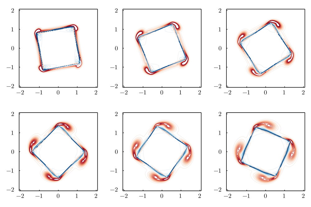
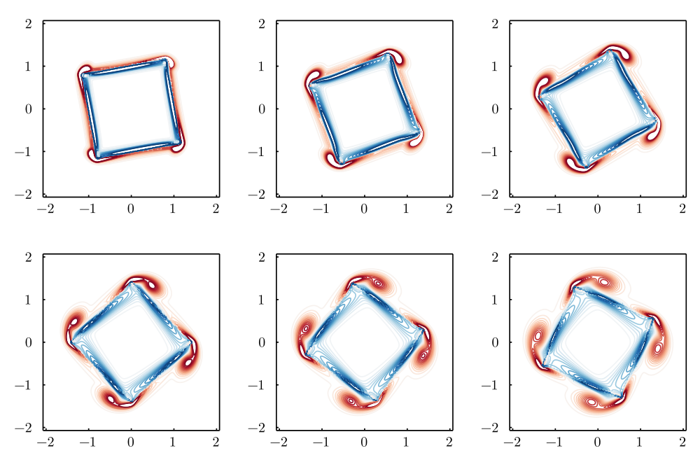
In the next example, we solve for the flow exterior to an impulsively-rotating square of side length $L$, at Reynolds number $\Omega L^{2}/\nu=400$. This case serves as a test of the discrete immersed layers to resolve the flow in the vicinity of a sharp corner. We use a grid spacing of $\Delta x/L=0.02$ and 260 forcing points distributed uniformly about the square’s perimeter; the time step size is set to $\nu\Delta t/\Delta x^{2}=0.25$ (or $\Omega\Delta t=0.01$). Figure 10 depicts the resulting vorticity using the current method. A small amount of vorticity is observed in the interior regions, but this leakage remains constant as the exterior vorticity develops due to flow separation from the corners. In contrast, the original IBPM [27, 19] generates an interior flow, as expected, shown in Figure 11.

References

- [1] E. Balaras and J. Yang. Nonboundary conforming methods for large-eddy simulations of biological flows. J. Fluids Eng., 127:851–857, 2005.
- [2] Horatio Scott Carslaw and John Conrad Jaeger. Conduction of Heat in Solids. Oxford University Press, 1959.
- [3] T. Colonius and K. Taira. A fast immersed boundary method using a nullspace approach and multi-domain far-field boundary conditions. Comput. Methods Appl. Mech. Engrg., 197:2131–2146, 2008.
- [4] Le Duan, Xiaowen Wang, and Xiaolin Zhong. A high-order cut-cell method for numerical simulation of hypersonic boundary-layer instability with surface roughness. J. Comput. Phys., 229(19):7207–7237, 2010.
- [5] Jeff D. Eldredge. ViscousFlow: A framework for simulating viscous incompressible flows about arbitrary body shapes. Zenodo. DOI: 10.5281/zenodo.4473257, 2021.
- [6] E. A. Fadlun, R. Verzicco, P. Orlandi, and J. Mohd-Yusof. Combined immersed-boundary finite-difference methods for three-dimensional complex flow simulations. J. Comput. Phys., 161:35–60, 2000.
- [7] F. Farassat. Introduction to Generalized Functions With Applications in Aerodynamics and Aeroacoustics. NASA Technical Paper 3428, 1996.
- [8] Ronald P. Fedkiw, Tariq Aslam, Barry Merriman, and Stanley Osher. A non-oscillatory Eulerian approach to interfaces in multimaterial flows (the ghost fluid method). J. Comput. Phys., 152(2):457–492, 1999.
- [9] Thomas Gillis, Grégoire Winckelmans, and Philippe Chatelain. Fast immersed interface Poisson solver for 3D unbounded problems around arbitrary geometries. J. Comput. Phys., 354:403–416, 2018.
- [10] R. Glowinski, T. W. Pan, and J. Périaux. Distributed Lagrange multiplier methods for incompressible viscous flow around moving rigid bodies. J. Comput. Phys., 151:181–194, 1998.
- [11] Andres Goza and Tim Colonius. A strongly-coupled immersed-boundary formulation for thin elastic structures. J. Comput. Phys., 336:401–411, 2017.
- [12] Andres Goza, Sebastian Liska, Benjamin Morley, and Tim Colonius. Accurate computation of surface stresses and forces with immersed boundary methods. J. Comput. Phys., 321:860–873, 2016.
- [13] Jungwoo Kim, Dongjoo Kim, and Haecheon Choi. An immersed-boundary finite-volume method for simulations of flow in complex geometries. J. Comput. Phys., 171(1):132–150, 2001.
- [14] Uǧis Lācis, Kunihiko Taira, and Shervin Bagheri. A stable fluid–structure-interaction solver for low-density rigid bodies using the immersed boundary projection method. J. Comput. Phys., 305:300–318, 2016.
- [15] M.-C. Lai and C. S. Peskin. An immersed boundary method with formal second-order accuracy and reduced numerical viscosity. J. Comput. Phys., 160:705–719, 2000.
- [16] L. Lee and R. J. LeVeque. An immersed boundary method for incompressible Navier–Stokes equations. SIAM J. Sci. Comput., 25:832–856, 2003.
- [17] R. J. Leveque and Z. Li. The immersed interface method for elliptic equations with discontinuous coefficients and singular sources. SIAM J. Num. Anal., 31(4):1019–1044, 1994.
- [18] S. Liska and T. Colonius. A fast lattice Green’s function method for solving viscous incompressible flows on unbounded domains. J. Comput. Phys., 316:360–384, 2016.
- [19] S. Liska and T. Colonius. A fast immersed boundary method for external incompressible viscous flows using lattice Green’s functions. J. Comput. Phys., 331:257–279, 2017.
- [20] Xu-Dong Liu, Ronald P. Fedkiw, and Myungjoo Kang. A boundary condition capturing method for Poisson’s equation on irregular domains. J. Comput. Phys., 160(1):151–178, 2000.
- [21] R. Mittal and G. Iaccarino. Immersed boundary methods. Annu. Rev. Fluid Mech., 37:239–61, 2005.
- [22] Rajat Mittal, Haibo Dong, Meliha Bozkurttas, FM Najjar, Abel Vargas, and Alfred Von Loebbecke. A versatile sharp interface immersed boundary method for incompressible flows with complex boundaries. J. Comput. Phys., 227(10):4825–4852, 2008.
- [23] C. S. Peskin. Numerical analysis of blood flow in the heart. J. Comput. Phys., 25:220–252, 1977.
- [24] C. S. Peskin and D. M. McQueen. A three-dimensional computational method for blood flow in the heart. I. Immersed elastic fibers in a viscous incompressible fluid. J. Comput. Phys., 81:372–405, 1989.
- [25] A. M. Roma, C. S. Peskin, and M. J. Berger. An adaptive version of the immersed boundary method. J. Comput. Phys., 153:509–534, 1999.
- [26] Ivar Stakgold. Boundary Value Problems of Mathematical Physics: Volume 2. SIAM, 2000.
- [27] K. Taira and T. Colonius. The immersed boundary method: a projection approach. J. Comput. Phys., 225:2118–2137, 2007.
- [28] Kunihiko Taira and Tim Colonius. Three-dimensional flows around low-aspect-ratio flat-plate wings at low Reynolds numbers. J. Fluid Mech., 623:187–207, 2009.
- [29] Hsieh-Chen Tsai and Tim Colonius. Coriolis effect on dynamic stall in a vertical axis wind turbine. AIAA Journal, 54(1):216–226, 2016.
- [30] H. S. Udaykumar, R. Mittal, P. Rampunggoon, and A. Khanna. A sharp interface Cartesian grid method for simulating flows with complex moving boundaries. J. Comput. Phys., 174:345–380, 2001.
- [31] C. Wang and J. D. Eldredge. Strongly coupled dynamics of fluids and rigid-body systems with the immersed boundary projection method. J. Comput. Phys., 295:87–113, 2015.
- [32] Xiaolei Yang, Xing Zhang, Zhilin Li, and Guo-Wei He. A smoothing technique for discrete delta functions with application to immersed boundary method in moving boundary simulations. J. Comput. Phys., 228(20):7821–7836, 2009.
- [33] Hong Zhao, Jonathan B. Freund, and Robert D. Moser. A fixed-mesh method for incompressible flow–structure systems with finite solid deformations. J. Comput. Phys., 227(6):3114–3140, 2008.