Zero-Sum Semi-Markov Games with State-Action-Dependent Discount Factors
Abstract
Semi-Markov model is one of the most general models for stochastic dynamic systems. This paper deals with a two-person zero-sum game for semi-Markov processes. We focus on the expected discounted payoff criterion with state-action-dependent discount factors. The state and action spaces are both Polish spaces, and the payoff function is -bounded. We first construct a fairly general model of semi-Markov games under a given semi-Markov kernel and a pair of strategies. Next, based on the standard regularity condition and the continuity-compactness condition for semi-Markov games, we derive a “drift condition” on the semi-Markov kernel and suppose that the discount factors have a positive lower bound, under which the existence of the value function and a pair of optimal stationary strategies of our semi-Markov game are proved by using the Shapley equation. Moreover, when the state and action spaces are both finite, a value iteration-type algorithm for computing the value function and -Nash equilibrium of the game is developed. The convergence of the algorithm is also proved. Finally, we conduct numerical examples to demonstrate our main results.
Keywords: Semi-Markov game, state-action-dependent discount factor, value iteration-type algorithm, -Nash equilibrium.
1 Introduction
Game theory is a fundamental mathematical model to study strategic interactions among rational decision-makers. It has wide applications in many fields, such as social science, computer science, management science, and economic systems. In the early period of game theory, it focuses on matrix games with two persons and zero sum, where each participant’s gains or losses are exactly balanced by those of the other. When the system state evolves over time, matrix games are transformed into two-person zero-sum stochastic games.
The study of zero-sum stochastic games is initiated by Shapley 1953, and many extensions of that work have been investigated in the literature. As is well known, it can be roughly classified into the following four main groups. The first group is discrete-time Markov games (Hernández-Lerma and Lasserre 2000; Küenle and Schurath 2003; Sennott 1994), which can be considered as an extension of discrete-time Markov control processes, that is, the decision epoch is the fixed discrete-time point and the state-action process is discrete. The second group deals with stochastic differential games (Basar 1999; Borkar and Ghosh 1996; Kushner 2003; Ramachandran 1999), where the evolution of state variables is governed by stochastic differential equations. The third group deals with continuous-time Markov games (Guo and Hernández-Lerma 2003; Guo and Hernández-Lerma 2005; Guo and Hernández-Lerma 2007; Neyman 2017) in which the sojourn times between consecutive decision epochs are exponentially distributed and the players can select their actions continuously in time. The fourth group is semi-Markov games (SMGs) (Jaskiewicz 2002; Lal and Sinha 1992; Luque-Vásquez 2002; Minjárez-Sosa and Luque-Vásquez 2008; Mondal et al. 2016), where the state process is continuous over time, the sojourn time between two consecutive decision epochs follows any distribution and players take actions just at the moment when the state changes.
In certain sense, we may argue that semi-Markov processes can model almost every possible stochastic dynamic system, since the sojourn time can be any distribution and the Markovian property can be satisfied by state augment. Therefore, it is important to study semi-Markov games which can be used to formulate wide varieties of decision-making problems in social and economic systems. In this paper, we focus on the study of two-person zero-sum SMGs. Lal and Sinha 1992 deal with two-person zero-sum SMGs under both expected discounted and long-run average payoff criterion, where the state space is denumerable and the payoff function is bounded. For the discounted case, they prove the existence of the value function and a pair of optimal stationary strategies by using the Shapley equation. For the long-run average case, they further establish the optimality equation and propose a standard ergodic condition under which the existence of the value function and a pair of optimal stationary strategies are ensured through solving the optimality equation in a unified manner. Jaskiewicz 2002 studies the two-person zero-sum SMGs under the long-run average payoff criterion with a more general model, where the state and action spaces are both Borel spaces and the payoff function is -bounded. This paper derives some generalized geometric ergodicity conditions on the transition probabilities under which the optimality equation has a solution which can be obtained by solving some -perturbed SGMs. This paper also proves the existence of the value function and a pair of optimal stationary strategies of the SMGs. There is further literature work on two-person zero-sum SMGs that extends the similar results to the expected discounted payoff criterion. Luque-Vásquez 2002 considers the -stage SMGs as well as the infinite horizon case with Borel state and action spaces and -bounded payoff function. The existence of the value function and a pair of optimal stationary strategies are also shown under suitable assumptions on the transition law. Moreover, Minjárez-Sosa and Luque-Vásquez 2008 study the discounted zero-sum SMGs with unknown holding time distribution for one player. They propose a state-action independent condition on to get independent observations during the evolution of the system, under which they combine suitable methods of statistical estimation of with control procedures to construct an asymptotically discount optimal pair of strategies.
Most of the literature work on game theory focuses on the existence of Nash equilibrium. However, how to efficiently solve a stochastic dynamic game and compute a pair of optimal stationary strategies are especially important for practical implementation of game theory. The classic algorithmic study on game theory focuses on static games, where the matrix game and the bimatrix game can be solved by linear programming and quadratic programming, respectively (Barron 2013). Recently, there are emerging investigations that aim to study the efficient computation for stochastic dynamic games using approximation or learning algorithms. Littman 1994 proposes a minimax-Q algorithm to solve discrete-time two-person zero-sum Markov games, which is essentially motivated by the standard Q-learning algorithm with a minimax operator in Markov games replacing the max operator in reinforcement learning. Al-Tamimi et al. 2007 utilize the method of Q-learning and approximate dynamic programming (ADP) to solve a discrete-time linear system quadratic zero-sum game, and the proof of the convergence of the algorithm is also given. Vamvoudakis and Lewis 2012 deal with a continuous-time two-person zero-sum game with infinite horizon cost for nonlinear systems with known dynamics. They propose a “synchronous” zero-sum game policy iteration algorithm to solve the game through learning the Hamilton-Jacobi-Isaacs (HJI) equation in real time. Moreover, a persistence of excitation condition is given under which the convergence to the optimal saddle point and the stability of the system are also guaranteed. Mondal et al. 2016 study the AR-AT (Additive Reward-Additive Transition) two-person zero-sum SMGs, where the state and action spaces are both finite. They prove that such game can be formulated as a vertical linear complementarity problem (VLCP), which can be solved by the Cottle-Dantzig’s algorithm.
All the above literature work on SMGs assumes that the discount factor is a constant, which may not always hold. For example, considering the application in economics, the discount factor (interest rate) may depend both on economy environments and decision-makers’ actions. That is, the interest rate usually varies in different financial markets and monetary policies, where financial markets can be considered as states and monetary policies are actions taken by the government. Thus, it is necessary and reasonable to study the SMGs with state-action-dependent discount factors. Problems with non-constant discount factors have been studied for Markov decision processes (MDP) (Minjárez-Sosa 2015; Ye and Guo 2012) and two-person zero-sum discrete-time Markov games (González-Sánchez et al. 2019). In this paper, we aim at studying the two-person zero-sum SMGs with expected discounted payoff criterion in which the discount factors are state-action-dependent. The objective is to find a pair of optimal strategies to maximize the payoff of player (P1) and minimize the payoff of player (P2). More precisely, we deal with the SMGs specified by five primitive data: the state space ; the action spaces for P1 and P2, respectively; the semi-Markov kernel ; the discount factor ; and the payoff function . The state space and action spaces are all Polish spaces, and the payoff function is -bounded. With these data, we construct an SMG model with a fairly general problem setting. Then we impose suitable conditions on the model parameters shown in Assumptions 1-4, under which we establish the Shapley equation and prove the existence of the value function and a pair of optimal stationary strategies of the game. Our proof is quite different from González-Sánchez et al. 2019 since we directly search for Nash equilibrium in history-dependent strategies instead of turning to Markov strategies. In addition, when the state and action spaces are both finite, we derive a value iteration-type algorithm to approach to the value function and Nash equilibrium of the game based on the Shapley equation. The convergence of the algorithm is also proved. Finally, we conduct numerical examples on investment problem to demonstrate the main results of our paper.
The contributions of this paper can be summarized as follows. (1) We construct the two-person zero-sum SMG model with expected discounted payoff criterion in which the discount factors are state-action-dependent. To the best of our knowledge, our work is the first one that the discount factor is regarded as a variable in stochastic semi-Markov games, which could complement the theoretical study on SMGs. (2) We derive a “drift condition” (see Assumption 3) on the semi-Markov kernel, which is more general than the counterpart in the literature work (Luque-Vásquez 2002), as stated in Remark 4. (3) We propose a value iteration-type algorithm to compute the value function and -Nash equilibrium of the SMG. This algorithm can be viewed as a combination of the value iteration of MDP and the linear programming of matrix games. Moreover, the convergence and the error-bound of the algorithm are also guaranteed.
The rest of this paper is organized as follows. In Section 2, we introduce the model of SMG as well as the optimality criterion. In Section 3, we impose suitable conditions on the model parameters under which the existence of the value function and a pair of optimal stationary strategies are proved by using the Shapley equation. A value iteration-type algorithm for computing the -Nash equilibrium is developed in Section 4, and some numerical examples are conducted to demonstrate our main results in Section 5. Finally, we conclude the paper and discuss some future research topics in Section 6.
2 Two-Person Zero-Sum Semi-Markov Game Model
Notation: If is a Polish space (that is, a complete and separable metric space), its Borel -algebra is denoted by , and denotes the family of probability measures on endowed with the topology of weak convergence.
In this section, we introduce a two-person zero-sum SMG model with expected discounted payoff criterion and state-action-dependent discount factors, which is denoted by the collection
where the symbols are explained as follows.
is the state space which is a Polish space, and and are action spaces for P1 and P2, respectively, which are also supposed to be Polish spaces.
and are Borel subsets of and , which represent the sets of the admissible actions for P1 and P2 at state , respectively. Let
be a measurable Borel subset of .
is a semi-Markov kernel which satisfies the following properties.
(a) For each fixed , is a probability measure on , whereas for each fixed , is a real-valued Borel function on .
(b) For each fixed and , is a non-decreasing right-continuous real-valued Borel function on such that .
(c) For each fixed ,
denotes the distribution function of the sojourn time at state when the actions are chosen. For each and , when P1 and P2 select actions and , respectively, denotes the joint probability that the sojourn time in state is not greater than and the next state belongs to D.
is a measurable function from to which denotes the state-action-dependent discount factor.
and are two real-valued functions on , which represent the payoff function for P1 and P2, respectively.
If for all , then the model is called a two-person zero-sum SMG. Otherwise, the game is nonzero-sum. In this paper, we focus on the zero-sum case. We denote , and regard P1 as the maximizer and P2 as the minimizer. The evolution of SMGs with the expected discounted payoff criterion carries on as follows.
Assume that the game starts at the initial state at the initial decision epoch . The two players choose simultaneously a pure action pair according to the variables and , then P1 and P2 receive immediate rewards , respectively. Consequently, after staying at state up to time , the system moves to a new state according to the transition law . Once the state transition to occurs at the st decision epoch , the entire process repeats again and the game evolves in this way.
Thus, we obtain an admissible history at the th decision epoch
When the game goes to infinity, we obtain the history
where , for all . Moreover, let be the class of all admissible histories of the system up to the th decision epoch, endowed with a Borel -algebra.
To introduce our expected discounted payoff criterion discussed in this paper, we give the definitions of strategies as follows.
Definition 1.
A randomized history-dependent strategy for P1 is a sequence of stochastic kernels that satisfies the following conditions:
(i) for each , is a Borel function on , and for each , is a probability measure on A;
(ii) is concentrated on , that is
We denote by the set of all the randomized history-dependent strategies for P1 for simplicity.
Definition 2.
(1) A strategy is called a randomized Markov strategy if there exists a sequence of stochastic kernels such that
(2) A randomized Markov strategy is called stationary if is independent of ; that is, if there exists a stochastic kernel on given such that
(3) Moreover, if is a Dirac measure for all , then the stationary strategy is called a pure strategy.
We denote by , and the sets of all the randomized Markov strategies, randomized stationary strategies and pure strategies for P1, respectively.
The sets of all randomized history-dependent strategies , randomized Markov strategies , randomized stationary strategies , pure strategies for P2 are defined similarly, with in lieu of . Clearly, and .
For each , by the Tulcea’s theorem (Hernández-Lerma and Lasserre 1996), there exists a unique probability space and a stochastic process such that for each and , we have
Corresponding to the stochastic process with probability space , we define an underlying continuous-time state-action process as
where , , are some isolated points, , and is an indicator function on any set .
Definition 3.
The stochastic process is called a semi-Markov game.
Next, we will show the definition of the expected discounted payoff criterion in this paper, where denotes the expectation operator associated with .
Definition 4.
For each , the initial state and discount factor , the expected discounted payoff criterion for player is defined as follows:
| (1) |
Remark 1.
Since , we just need to consider the expected discounted payoff criterion for P1. Let
This paper focuses on the study of the value function and Nash equilibrium of the SMG. So we need the following concepts.
Definition 5.
The upper value and lower value of the expected discounted payoff SMG are defined as
respectively. Obviously, for all . Moreover, if it holds that for all , then the common function is called the value function of the game and denoted by .
Definition 6.
Assume that the game has a value . Then a strategy is said to be optimal for P1 if
Similarly, is said to be optimal for P2 if
If is optimal for player (), then we can call a pair of optimal strategies (Nash equilibrium).
Remark 2.
is a pair of optimal strategies if and only if
Remark 2 is an effective method to verify whether a pair of strategy is a Nash equilibrium, which is widely used in the literature; see, for instance, Luque-Vásquez 2002, and the references therein.
3 Optimality Analysis
In this section, we give some suitable assumptions on the model parameters under which the existence of the value function and a pair of optimal stationary strategies are guaranteed. The related proofs are also discussed.
Given a measurable function , a function on is said to be -bounded if it has finite -norm which is defined as
such a function can be referred to as a weight function. For convenience, we write the Banach space of all -bounded measurable functions on .
Next, we give some hypotheses to guarantee the existence of a pair of optimal strategies.
Assumption 1.
There exist constants and such that
Remark 3.
Assumption 1 is a regularity condition which indicates that for each fixed and , we have
which avoids possibility of infinitely many decision epochs during the finite time interval; see, for instance, Lal and Sinha 1992, Luque-Vásquez 2002, and the references therein .
To guarantee the finiteness of the expected discounted payoff defined in (1), we propose the following assumption.
Assumption 2.
(a) There exists a constant such that for all . (b) There exists a measurable function and a nonnegative constant such that for all ,
Lemma 1.
Proof.
Assumption 3.
There exists a constant with such that for all fixed and ,
| (3) |
where is the function mentioned in Assumption 2.
Remark 4.
We call Assumption 3 the “drift condition”, which is needed to ensure that the Shapley operator (defined later in (6)) is a contraction operator as well as our main results. Particularly, if , where denotes the state transition probability, (3) degenerates into , which is the same as the Assumption 3(b) of Luque-Vásquez 2002. Thus, our Assumption 3 is more general than the counterpart in the literature Luque-Vásquez 2002.
Moreover, we impose the following continuity-compactness conditions to ensure the existence of a pair of optimal stationary strategies of our SMG model.
Assumption 4.
(a) For each fixed , and are both compact sets.
(b) For each fixed , is upper semi-continuous on and is lower semi-continuous on .
(c) For each fixed , and , the functions
are continuous on and , respectively.
(d) For each fixed , is continuous on .
(e) The function is continuous on .
Remark 5.
Assumption 4 is similar to the standard continuity-compactness hypotheses for Markov control processes; see, for instance, Hernández-Lerma and Lasserre 1999, and the references therein. It is commonly used for the existence of minmax points of games.
By Lemma in Nowak 1984, if Assumption 4(a) holds, then the probability spaces are also compact for each .
We now introduce the following notations: for each given function and , we write
| (5) |
For each fixed and probability measures , we denote
whenever the integral is well defined.
We define an operator on by
| (6) |
which is called the Shapley operator. A function is said to be a solution of the Shapley equation if
In order to explore the existence of a pair of optimal stationary strategies, we also need to define another operator on by
where is a pair of stationary strategies.
Before stating our main results, we need the following lemmas:
Lemma 2.
Proof.
By Assumption 2 and formulation (4), for each given function and , we can easily get
The above inequality yields , which implies is in , and so .
On the one hand, by Assumption 4, it follows that is upper semi-continuous in , then for each fixed , by the Fatou’s theorem, the function
is also upper semi-continuous in . Moreover, since the probability measures on endowed with the topology of weak convergence, by Theorem in Ash et al. 2000, the function is upper semi-continuous in . Similarly, is lower semi-continuous in . Thus, by Theorem in Ash et al. 2000, the supremum and the infimum are indeed attained in (6), which means
Then, by the Fan’s minimax Theorem (Fan 1953), we obtain (7).
On the other hand, it is clear that is both concave and convex in with respect to and in with respect to . Hence, by the well-known measurable selection theorem (Nowak 1985), there exists a pair of stationary strategies that satisfies (8). ∎
Lemma 3.
Both and are contraction operators with modulus less than .
Proof.
First, it is easy to verify that the operator is monotonically increasing. Let , by the definition of -norm, , it follows that for each fixed , we have
| (9) | ||||
where the last inequality is followed by formulation (4). Furthermore, taking maximum of and minimum of on both sides of the inequality (9), we have
i.e.
Similarly, interchanging and , we obtain
Combining the two inequalities above, we have
i.e.
which implies is a contraction operator with modulus . Using the same arguments, we can prove that is also a contraction operator with modulus . ∎
Since and are both contraction operators, then there exist unique functions and such that and by the Banach’s fixed point theorem.
Lemma 4.
For each and ,
where , and which denotes the translation of strategy.
Proof.
where the third and fourth equalities are ensured by the property of conditional expectation. The fifth equality follows from the strong Markovian property. Hence,
which is required. ∎
Now, if we set and specially, which are both stationary strategies, from Lemma 4, we have
which implies that the function is the unique fixed point of the contraction operator .
Proof.
Next, we present our main results.
Theorem 1.
(a) The semi-Markov game has a value function , which is the unique function in that satisfies the Shapley equation
and furthermore, there exists a pair of optimal strategies.
(b) A pair of stationary strategies is optimal if and only if its expected payoff satisfies the Shapley equation for all .
Proof.
(a) Let be the unique fixed point of in , that is
By Lemma 2, there exists a pair of stationary strategies such that for each ,
| (10) | ||||
which implies that
Moreover, by Lemma 4,
from which we can derive
Next, we prove that is the value function of the game and is a pair of optimal strategies, that is
| (11) |
We first prove the first inequality in (11). Then a similar proof can follow for the second inequality. By (10), we have
Particularly, let be an indicator function such that . Then for each , we have
taking as a random variable , then for all , we have
For , integrating on both sides in the above inequality, we have
Multiplying on both sides in the above inequality and using the properties of the conditional expectation, we have
Then, taking the expectation , we have
Now, summing over , we obtain
Letting , according to Lemma 5, we derive
which means that the first inequality in (11) holds.
(b) ()
Suppose that is a pair of optimal stationary strategies, then for each , we have
For each fixed , let with and , then by Lemma 4, for each , we have
which yields
Similarly, we can prove
Combining the last two inequalities, we obtain the desired result.
()
This part holds, which has been proved in part . ∎
4 Algorithm
In this section, we develop an iterative algorithm to approach to the value function and Nash equilibrium of our two-person zero-sum stochastic SMG, where numerically solving matrix games is iteratively utilized at every state in a form of value iteration. First, we introduce some concepts about matrix games (Barron 2013).
A two-person zero-sum static game in a matrix form means that there is a matrix of real numbers so that if P1, the row player chooses to play row , while P2, the column player chooses to play column , then the payoff to P1 is and the payoff to P2 is . Every row and column represents a pure strategy adopted by P1 and P2, respectively. Both players aim to choose strategies that maximize their individual payoffs. To guarantee the optimality, we have to consider mixed strategies, where a player chooses a row or column according to some probability distributions.
Definition 7.
A mixed strategy is a vector for P1, and for P2, where
The components and represent the probabilities that row will be chosen by P1 and column will be chosen by P2, respectively. Denote the set of mixed strategies with components by
Definition 8.
Let be a mixed strategy for P1, and be a mixed strategy for P2, then the expected payoff to P1 is
In a two-person zero-sum game, the expected payoff to P2 is .
Both players aim to choose strategies that maximize their individual payoffs. P1 wants to choose a strategy to maximize the payoff in the matrix, while P2 wants to choose a strategy to minimize the payoff in the matrix.
Definition 9.
The upper and lower values of the matrix game are defined as
If , then the common value is called the value of the game and denoted by .
Moreover, a saddle point in mixed strategies is a pair , which satisfies
By Theorem in Barron 2013, we know that any matrix game has a unique value as well as at least one saddle point. There is a method of formulating the matrix game as a linear program as follows (Barron 2013):
P1 aims to choose a mixed strategy to maximize the payoff
| (12) |
P2 aims to choose a mixed strategy to minimize the payoff
We can use the classic algorithms to solve the two linear programs (12) and (4), such as simplex method or interior point method. Note that the optimal values of solved by (12) and (4) are always equal. Therefore, the optimal strategies of P1 and P2 and the value of the game can be obtained in a straightforward way.
Next, we utilize the above technique of solving matrix games to study the computation of two-person zero-sum stochastic SMGs, where a value iteration-type algorithm is developed to approach to the value function and Nash equilibrium . To this end, we need to introduce the following concept.
Definition 10.
Assume that the SMG has a value function . Then a pair of strategies is said to be an -Nash equilibrium of the game if
Moreover, is called the -value function of the game.
Consider the mathematical model of SMG discussed in this paper. In order to numerically approach to the value function and Nash equilibrium, we simplify the general state and action spaces as finite case for convenience. Without loss of generality, we assume that and , for any . Under Assumptions 1-4 mentioned in Section 3, we obtain the Shapley equation as follows
| (18) |
For each fixed and given function , let be an -dimensional matrix with elements defined as
where is defined in (5). We further define as an -dimensional vector and as an -dimensional vector, which are all mixed strategies. According to (4), we have
| (19) |
which can be viewed as a matrix game for the value function at each state .
However, we cannot directly solve (19) since the value function is unknown. Below, we develop Algorithm 1 to iteratively compute a series of matrix games whose values can asymptotically approach to at each state . From the lines 11-12 of Algorithm 1, we can see that at the th iteration, we can obtain and by using linear programming (12) and (4) to solve the game with matrix whose element is , where , , , and . This iterative procedure of computing a series of is similar to the classic value iteration algorithm in the MDP theory. Furthermore, we give a theorem (Theorem 2) to prove the convergence of Algorithm 1.
Initialize: for all arbitrarily
repeat 1
Loop for each do 2
for do 3
until ; 5
and
Remark 6.
Theorem 2.
Proof.
According to the iterative formula of Algorithm 1, we have
which by iteration yields
For each given and initial value , if , choose , and we have
otherwise, if , choose , and we have
Combining the two cases above, choose and we have , which implies that Algorithm 1 can converge within iterations.
Moreover, since is the unique solution of the Shapley equation, we have
thus,
taking , and we have
which implies that is an -Nash equilibrium by Definition 10. ∎
Therefore, with Algorithm 1, we can iteratively approach to the value function and Nash equilibrium of our SMG problem through recursively solving linear programming (12) and (4) at each state . Theorem 2 guarantees the convergence of Algorithm 1. We can implement Algorithm 1 with discretization techniques for computers to solve practical problems, as illustrated in the next section.
5 Numerical Experiment
In this section, we conduct numerical examples to illustrate our main results derived in Sections 3&4. First, we give an example to demonstrate that Assumptions 1-4 ensuring the existence of the value function and Nash equilibrium of SMGs are easy to verify in practice.
Example 1.
Consider a system with a model of SMG which is defined as follows:
The state space and the action spaces with admissible action sets for each . The semi-Markov kernel is given by:
where is a positive constant and is a probability distribution. The payoff function is denoted by which is bounded. Moreover, the discount factor is defined as .
Now, we verify that the conditions on the existence of a pair of optimal stationary strategies described in Assumptions 1-4 are satisfied in this example. To this end, we need the following hypothesis:
Assumption 5.
There exist positive constants and such that for each , we have for each and for each .
With this hypothesis, we directly have the following result.
Proposition 1.
Proof.
Obviously, Assumption 2 holds by choosing and . Since and are discrete, Assumption 4 holds. Next we verify Assumptions 1&3. According to the semi-Markov kernel , we have
Let and , we have that
if ,
if ,
which implies that Assumption 1 holds.
By Lemma 1, we derive
Next, we give another example about investment problem to demonstrate the numerical computation of Algorithm 1 to solve the value function and a pair of optimal stationary strategies of the game.
Example 2.
Consider an investment problem with three states , which denotes the benefit, medium and loss economy environments, respectively. At each state, the investor will buy some assets while the market-maker will sell. The interest rate depends on the economy environments as well as the number of assets that investor buys and market-maker sells. In state , the investor buys a certain amount of assets from and the market-maker sells from , which leads to a payoff to the investor and to the market-maker, where . Then the system moves to a new state with probability after staying at state for a random time which follows exponential-distribution with parameter . In state , the investor buys a certain amount of assets from and the market-maker sells from , which leads to a payoff to the investor and to the market-maker, where . Then the system moves to a new state with probability after staying at state for a random time uniformly distributed in with parameter . For this system, the decision makers aim to find a pair of optimal strategies.
First, we establish a model of SMG for this example as follows.
We set , , for each and the semi-Markov kernel is given by:
from which we can obtain
and
Then by (5), we have
To take numerical calculation for this example, we assume that the values of model parameters are shown in Table 1.
| state | 1 | 2 | 3 | |||||||||||||||||||||||||||||||||
|---|---|---|---|---|---|---|---|---|---|---|---|---|---|---|---|---|---|---|---|---|---|---|---|---|---|---|---|---|---|---|---|---|---|---|---|---|
| action |
|
|
|
|
|
|
|
|
|
|
|
| ||||||||||||||||||||||||
| 0.98 | 0.96 | 0.92 | 0.9 | 0.78 | 0.76 | 0.73 | 0.7 | 0.86 | 0.84 | 0.89 | 0.82 | |||||||||||||||||||||||||
| 40 | 24 | 18 | 33 | 12 | 8 | 10 | 17 | 3 | 5 | 2 | 6 | |||||||||||||||||||||||||
| 20 | 30 | 11 | 13 | 7 | 8 | 6.5 | 4 | 0.34 | 0.44 | 0.55 | 0.15 | |||||||||||||||||||||||||
| 0 | 0 | 0 | 0 | 0.46 | 0.48 | 0.39 | 0.3 | 0.45 | 0.24 | 0.43 | 0.4 | |||||||||||||||||||||||||
| 0.5 | 0.43 | 0.32 | 0.62 | 0 | 0 | 0 | 0 | 0.55 | 0.76 | 0.57 | 0.6 | |||||||||||||||||||||||||
| 0.5 | 0.57 | 0.68 | 0.38 | 0.54 | 0.52 | 0.61 | 0.7 | 0 | 0 | 0 | 0 | |||||||||||||||||||||||||
Under these data, we can verify that Assumptions 1-4 hold by using Proposition 1. Thus, the existence of the value function and Nash equilibrium of the SMG are ensured by Theorem 1. Moreover, by Assumption 5 and proposition 1, we can choose , from which we obtain . Next, we use Algorithm 1 to find the value function and a pair of optimal stationary strategies of the game. The detailed steps are listed as follows.
Step 1: Initialization.
Let , and ; set a small threshold , and we have .
Step 2: Iteration.
For , , we have
Then, for each state , we solve the linear program
| (23) |
with the solution denoted by where , .
Step 3: Termination judgement.
If , then the iteration stops, is the -value function and is -Nash equilibrium of the SMG; Otherwise, set and go to Step 2.
We use Matlab to implement the iteration algorithm for this example. It takes about seconds to stop at the rd iteration. The curves of the error of two successive iterations, the value function, and the strategy pair of players with respect to the iteration times are illustrated by Figures 2-3.
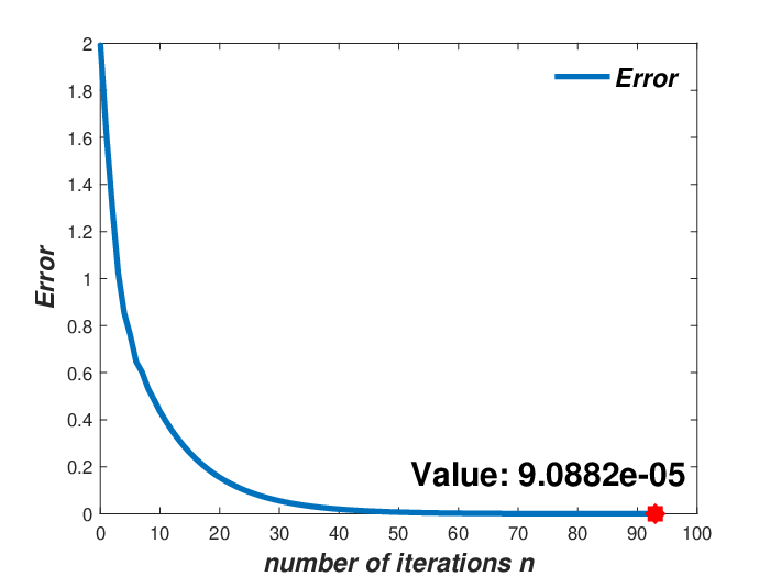


Based on the experimental results, we have the following observations:
When the state is benefit, the investor should take action with probability and with probability , while the market-maker should take action with probability and with probability ;
When the state is medium, the investor should take action with probability and with probability , while the market-maker should take action with probability and with probability ;
When the state is loss, the investor should always take action while the market-maker should always take action ;
If both investor and market-maker use the optimal strategies, the investor will obtain a profit at benefit state, at medium state and at loss state, while the market-maker will lose the same amount, respectively.
Remark 7.
In this example, we choose a uniformly distributed sojourn time at state to show that arbitrary distributions are permitted for the sojourn time of semi-Markov processes. Other distributions can also be chosen for the sojourn time according to practical situations. Moreover, if all the sojourn times are exponentially distributed, the semi-Markov games degenerate into discrete-time Markov games.
6 Conclusion
In this paper, we concentrate on the two-person zero-sum SMG with expected discounted payoff criterion in which the discount factors are state-action-dependent. We first construct the SMG model with a fairly general definition setting. Then we impose suitable conditions on the model parameters, under which we establish the Shapley equation whose unique solution is the value function and prove the existence of a pair of optimal stationary strategies of the game. While the state and action spaces are finite, a value iteration-type algorithm for approaching to the value function and Nash Equilibrium is developed. Finally, we apply our results to an investment problem, which demonstrates that our algorithm performs well.
One of the future research topics is to deal with the nonzero-sum case of this game model. We wish to find sufficient conditions under which we use the similar arguments to establish the Shapley equation and prove the existence of a pair of optimal stationary strategies for such game. In addition to the value iteration algorithm, the policy iteration algorithm is also widely used to solve MDPs. Therefore, it is also promising to develop a policy iteration-type algorithm to solve the two-person zero-sum SMGs. Moreover, considering the limitations of computing resources, the dynamic programming algorithm is difficult to implement in reality when the scale of the game becomes huge. Another future research topic is to develop data-driven learning algorithms to approximately solve the game problems, such as the combination with multi-agent reinforcement learning approaches.
Acknowledgements
This work was supported in part by the National Natural Science Foundation of China (11931018, 61573206).
References
- Al-Tamimi et al. (2007) Al-Tamimi A, Lewis FL, Abu-Khalaf M (2007) Model-free Q-learning designs for linear discrete-time zero-sum games with application to H-infinity control.Automatica 43(3):473–481
- Ash et al. (2000) Ash RB, Robert B, Doleans-Dade CA, Catherine A (2000) Probability and Measure Theory. Academic Press
- Barron (2013) Barron EN (2013) Game Theory: An Introduction, vol 2. John Wiley & Sons
- Basar (1999) Basar T (1999) Nash equilibria of risk-sensitive nonlinear stochastic differential games. Journal of Optimization Theory and Applications 100(3):479–498
- Borkar and Ghosh (1996) Borkar VS, Ghosh MK (1996) Stochastic differential games: occupation measure based approach. Journal of Optimization Theory and Applications 88(1):251–252
- Fan (1953) Fan K (1953) Minimax theorems. Proceedings of the National Academy of Sciences of the United States of America 39(1):42–47
- González-Sánchez et al. (2019) González-Sánchez D, Luque-Vásquez F, Minjárez-Sosa JA (2019) Zero-Sum Markov Games with Random State-Actions-Dependent Discount Factors: Existence of Optimal Strategies. Dynamic Games and Applications 9(1):103–121
- Guo and Hernández-Lerma (2003) Guo X, Hernández-Lerma O (2003) Zero-sum games for continuous-time Markov chains with unbounded transition and average payoff rates. Journal of Applied Probability 40(2):327–345
- Guo and Hernández-Lerma (2005) Guo X, Hernández-Lerma O (2005) Zero-sum continuous-time Markov games with unbounded transition and discounted payoff rates. Bernoulli 11(6):1009–1029
- Guo and Hernández-Lerma (2007) Guo X, Hernández-Lerma O (2007) Zero-sum games for continuous-time jump Markov processes in Polish spaces: discounted payoffs. Advances in Applied Probability 39(3):645–668
- Hernández-Lerma and Lasserre (1996) Hernández-Lerma O, Lasserre JB (1996) Discrete-Time Markov Control Processes. Springer Science & Business Media
- Hernández-Lerma and Lasserre (1999) Hernández-Lerma O, Lasserre JB (1999) Further Topics on Discrete-Time Markov Control Processes. Springer Science & Business Media
- Hernández-Lerma and Lasserre (2000) Hernández-Lerma O, Lasserre JB (2000) Zero-sum stochastic games in Borel spaces: average payoff criteria. SIAM Journal on Control and Optimization 39(5):1520–1539
- Jaskiewicz (2002) Jaskiewicz A (2002) Zero-sum semi-Markov games. SIAM Journal on Control and Optimization 41(3):723–739
- Küenle and Schurath (2003) Küenle HU, Schurath R (2003) The optimality equation and -optimal strategies in Markov games with average reward criterion. Mathematical Methods of Operations Research 56(3):451–471
- Kushner (2003) Kushner HJ (2003) Numerical approximations for stochastic differential games: the ergodic case. SIAM Journal on Control and Optimization 42(6):1911–1933
- Lal and Sinha (1992) Lal AK, Sinha S (1992) Zero-sum two-person semi-Markov games. Journal of Applied Probability 29(1):56–72
- Littman (1994) Littman ML (1994) Markov games as a framework for multi-agent reinforcement learning. In: Machine Learning Proceedings, Elsevier, pp 157–163
- Luque-Vásquez (2002) Luque-Vásquez F (2002) Zero-sum semi-Markov game in Borel spaces with discounted payoff. Morfismos 6(1):15–29
- Minjárez-Sosa (2015) Minjárez-Sosa JA (2015) Markov control models with unknown random state–action-dependent discount factors. Top 23(3):743–772
- Minjárez-Sosa and Luque-Vásquez (2008) Minjárez-Sosa JA, Luque-Vásquez F (2008) Two person zero-sum semi-Markov games with unknown holding times distribution on one side: a discounted payoff criterion. Applied Mathematics and Optimization 57(3):289–305
- Mondal et al. (2016) Mondal P, Sinha S, Neogy SK, Das AK (2016) On discounted AR–AT semi-Markov games and its complementarity formulations. International Journal of Game Theory 45(3):567–583
- Neyman (2017) Neyman A (2017) Continuous-time stochastic games. Games and Economic Behavior 104:92–130
- Nowak (1984) Nowak AS (1984) On zero-sum stochastic games with general state space I.Probability and Mathematical Statistics 4(1):13–32
- Nowak (1985) Nowak AS (1985) Measurable selection theorems for minimax stochastic optimization problems. SIAM Journal on Control and Optimization 23(3):466–476
- Ramachandran (1999) Ramachandran K (1999) A convergence method for stochastic differential games with a small parameter. Stochastic Analysis and Applications 17(2):219–252
- Sennott (1994) Sennott LI (1994) Zero-sum stochastic games with unbounded costs: discounted and average cost cases. Zeitschrift für Operations Research 39(2):209–225
- Shapley (1953) Shapley LS (1953) Stochastic games. Proceedings of the National Academy of Sciences 39(10):1095–1100
- Vamvoudakis and Lewis (2012) Vamvoudakis KG, Lewis FL (2012) Online solution of nonlinear two-player zero-sum games using synchronous policy iteration. International Journal of Robust and Nonlinear Control 22(13):1460–1483
- Ye and Guo (2012) Ye L, Guo X (2012) Continuous-time Markov decision processes with state-dependent discount factors. Acta Applicandae Mathematicae 121(1):5–27