跳到论文正文
W Papers独立论文阅读器 arXiv:2103.03801 论文正文 计算阅读时间 · 0%
引用这篇论文根据当前论文元数据生成,正式投稿前建议核对。


License: CC Zero
arXiv:2103.03801v1 [cs.IT] 05 Mar 2021

Error-Correction for Sparse
Support Recovery Algorithms

Mohammad Mehrabi    Aslan Tchamkerten Thanks: M. Mehrabi is with the Data Sciences and Operations Department, Marshall School of Business, University of Southern California, Los Angeles, CA 90089-0809, US. Thanks: A. Tchamkerten is with the Department of Communications and Electronics, Telecom Paris, Institut Polytechnique de Paris, 19 Place Marguerite Perey, 91120 Palaiseau, FR.
Abstract

Consider the compressed sensing setup where the support 𝐬∗\mathbf{s}^{*} of an mm-sparse dd-dimensional signal 𝐱\mathbf{x} is to be recovered from nn linear measurements with a given algorithm. Suppose that the measurements are such that the algorithm does not guarantee perfect support recovery and that true features may be missed. Can they efficiently be retrieved?

This paper addresses this question through a simple error-correction module referred to as LiRE. LiRE takes as input an estimate 𝐬in\mathbf{s}_{\text{in}} of the true support 𝐬∗\mathbf{s}^{*}, and outputs a refined support estimate 𝐬out\mathbf{s}_{\text{out}}. In the noiseless measurement setup, sufficient conditions are established under which LiRE is guaranteed to recover the entire support, that is 𝐬out⊇𝐬∗\mathbf{s}_{\text{out}}\supseteq\mathbf{s}^{*}. These conditions imply, for instance, that in the high-dimensional regime LiRE can correct a sublinear in mm number of errors made by Orthogonal Matching Pursuit (OMP). The computational complexity of LiRE is 𝒪⁡(m​n​d){\cal{O}}(mnd).

Experimental results with random Gaussian design matrices show that LiRE substantially reduces the number of measurements needed for perfect support recovery via Compressive Sampling Matching Pursuit, Basis Pursuit (BP), and OMP. Interestingly, adding LiRE to OMP yields a support recovery procedure that is more accurate and significantly faster than BP. This observation carries over in the noisy measurement setup where the combination of LiRE and OMP is faster and more accurate than LASSO. Finally, as a standalone support recovery algorithm with a random initialization, experiments show that LiRE’s reconstruction performance lies between OMP and BP.

These results suggest that LiRE may be used generically, on top of any suboptimal baseline support recovery algorithm, to improve support recovery or to operate with a smaller number of measurements, at the cost of a relatively small computational overhead. Alternatively, LiRE may be used as a standalone support recovery algorithm that is competitive with respect to OMP.

Index Terms: 
Compressed sensing, error-correction, feature selection, high dimension, linear model, support recovery

I Introduction

Consider the support recovery problem of an mm-sparse signal 𝐱∗∈ℝd\mathbf{x}^{*}\in{\mathbb{R}}^{d} from n<dn<d linear measurements:

𝐲=𝚽​𝐱∗,\displaystyle{\mathbf{y}}={\mathbf{\Phi}}\mathbf{x}^{*}, (1)

where 𝚽∈ℝn×d{\mathbf{\Phi}}\in{\mathbb{R}}^{n\times d} refers to the design matrix. Suppose an algorithm AA is used to recover the support 𝐬∗\mathbf{s}^{*} of 𝐱∗\mathbf{x}^{*} in a regime where errors may happen; for instance, the Restricted Isometry Property (RIP) constant of 𝚽{\mathbf{\Phi}} need not be small enough to guarantee perfect support recovery—see, e.g., [1] for such a condition for OMP. Can potential errors be efficiently corrected?

We address this question through a simple low complexity error-correction module, referred to as LiRE—for List Regression Error-correction. LiRE takes as input an initial support estimate

𝐬in​=def​A​(𝐲,𝚽)\mathbf{s}_{\text{in}}\overset{\text{def}}{=}A({\mathbf{y}},{\mathbf{\Phi}})

provided by a baseline algorithm AA, and produces a second support estimate

𝐬out​=def​LiRE​(𝐲,𝐬in,𝚽)​=notation​LiRE∘A⁡(𝐲,𝚽)\mathbf{s}_{\text{out}}\overset{\text{def}}{=}\text{LiRE}({\mathbf{y}},\mathbf{s}_{\text{in}},{\mathbf{\Phi}})\overset{\text{notation}}{=}\text{LiRE}\circ A({\mathbf{y}},{\mathbf{\Phi}})

of size mm. Under certain RIP conditions that depend on the number of missed features |𝐬∗\𝐬in||\mathbf{s}^{*}\backslash\mathbf{s}_{\text{in}}|, LiRE’s estimate 𝐬out\mathbf{s}_{\text{out}} includes 𝐬∗\mathbf{s}^{*} (see Theorem 1 and Corollaries 1,2 in Section II). In the high-dimensional regime, these conditions imply, for instance, that we can use OMP in a regime where perfect support recovery is not guaranteed, and yet LiRE will recover all missed features as long as their number grows sublinearly in the sparsity level.

In a second part of the paper, we further assess the performance of LiRE first as an error-correction module, then as a standalone support recovery algorithm with a random initialization. We present four sets of numerical experiments that address the following questions: Can LiRE improve the support recovery of (good) baseline algorithms? Can LiRE be combined with a baseline algorithm of similarly low complexity to achieve the performance of more complex reconstruction algorithms? Is LiRE robust to noise? And, how efficient is LiRE as a standalone support recovery algorithm? These questions are addressed by considering random Gaussian supports and design matrices.

  • •

    The first experiment considers OMP, BP ([2]), and Compressive Sampling Matching Pursuit (CoSaMP, [3]) as baseline algorithms. Results show that a few (five) iterations of LiRE increases and never decreases the average percentage of exact support recovery, for a non-trivial range of undersampling-sparsity operating regimes. In particular, LiRE reduces the number of measurements needed for perfect support recovery via CoSaMP, BP, and OMP by up to 15%15\%, 25%25\%, and 40%40\%, respectively, depending on the the sparsity level.

  • •

    The second set of simulations compares LiRE∘\circOMP against BP and shows that even though LiRE∘\circOMP has a significantly lower complexity than BP (𝒪⁡(m​n​d){\mathcal{O}}(mnd) vs. 𝒪⁡(n2​d1.5){\mathcal{O}}(n^{2}d^{1.5}), see [4]), it achieves an average percentage of successful support recovery that is at least as large as BP, and sometimes larger.

  • •

    The third set of simulations evaluates the robustness of LiRE against noise in the Gaussian additive model

    𝐲=𝚽​𝐱∗+𝐳.{\mathbf{y}}={\mathbf{\Phi}}\mathbf{x}^{*}+{\mathbf{z}}.

    By repeating the second set of experiments but now with LiRE∘\circOMP against the LASSO solution, we observe that LiRE∘\circOMP is superior to LASSO as the noise level increases even though computing the LASSO has a computational cost that is at least quadratic in dd [5].

  • •

    The fourth set of simulations evaluates the performance of LiRE as a standalone support recovery algorithm with a random initialization. Results show that in terms of percentage of exact support recovery LiRE lies between OMP and BP.

I-A Related works

The problem of solving the under-determined system of equations given by (1) to recover the planted solution 𝐱∗\mathbf{x}^{*}, a.k.a. compressed sensing, has a vast literature. By assuming some structural properties of 𝐱∗\mathbf{x}^{*}, there exists a unique solution to (1) which may be found efficiently depending on 𝚽{\mathbf{\Phi}}. The most common property is that 𝐱∗\mathbf{x}^{*} is m−m-sparse. Finding the sparsest solution

min𝐱:𝚽​𝐱=𝐲||𝐱||0\min_{\mathbf{x}:{\mathbf{\Phi}}\mathbf{x}={\mathbf{y}}}||\mathbf{x}||_{0}

is a non-convex NP-hard problem [6], but convex optimization can recover 𝐱∗\mathbf{x}^{*} if the design matrix 𝚽{\mathbf{\Phi}} satisfies certain conditions. For instance, in [7] it is shown that if 𝚽{\mathbf{\Phi}} satisfies a certain RIP condition, then the sparsest solution corresponds to 𝐱∗\mathbf{x}^{*} but also corresponds to the solution of the convex optimization problem min𝐱:𝚽​𝐱=𝐲||𝐱||1\min_{\mathbf{x}:{\mathbf{\Phi}}\mathbf{x}={\mathbf{y}}}||\mathbf{x}||_{1}, a.k.a. Basis Pursuit. For alternative structural properties and related conditions see, e.g., [8, 9, 10].

Over the past fifteen years, a significant amount of work has gone into the design of ever more efficient reconstruction algorithms, and conditions on 𝚽{\mathbf{\Phi}} under which reconstruction is possible, see, e.g., [2, 11, 3, 12, 13, 14, 15, 16, 17]. The performance of these algorithms is typically quantified in terms of computational complexity and the sparsity-undersampling tradeoff, that is the nn vs. mm curve (at fixed dd) that characterizes the regimes where support recovery is attained, possibly within some prescribed distortion [18, 7, 19, 20, 21, 22, 23, 24, 25]. Recall that in high dimensions (say, d=ω⁡(n3)d=\omega(n^{3})), the computational bottleneck for computing 𝐱∗\mathbf{x}^{*} lies in finding 𝐬∗\mathbf{s}^{*}. Given 𝐬∗\mathbf{s}^{*}, the signal 𝐱∗\mathbf{x}^{*} is obtained by minimizing ‖𝐲−𝚽​𝐱‖2||{\mathbf{y}}-{\mathbf{\Phi}}\mathbf{x}||_{2} over all 𝐱\mathbf{x} with support 𝐬∗\mathbf{s}^{*}. In turn, this least square estimate is equal to Penrose’s pseudo-inverse 𝚽†{\mathbf{\Phi}}^{\dagger} of 𝚽{\mathbf{\Phi}} applied to 𝐲{\mathbf{y}}, which can be performed with order 𝒪⁡(m2​n){\mathcal{O}}(m^{2}n) computations using direct methods (e.g., QR factorization) or cost 𝒪⁡(m​n){\mathcal{O}}(mn) using approximation methods, e.g., Richardson’s method (see, e.g., [3, Section 5.1]).

There are two main categories of signal reconstruction algorithms. In the first category, algorithms attempt to solve a convex relaxation of the original non-convex optimization problem, similarly to BP. In the second category, a support estimate is first constructed, typically in an iterative and greedy manner, then the signal is estimated. Prominent algorithms here include OMP and CoSaMP. It is generally accepted that algorithms based on convex relaxations achieve better sparsity-undersampling performance than greedy algorithms at the cost of an increase in computational complexity—see, for instance, [26] for complexity/performance comparison of BP and OMP. Beyond greedy algorithms and in the quest of ever faster reconstruction algorithms, a line of works takes advantage of distributed and parallel computation to further reduce computational time (see, e.g., [27, 28]).

Although many recovery algorithms have been shown to perform well in certain settings, the tradeoff between reconstruction performance and computational complexity remains elusive in general. The present work is a further exploration of this tradeoff by providing a means to increase reconstruction performance at the cost of a relatively small computational overhead.

Remark.

This paper is an extended version of the ISIT 20212021 conference submission [29]. The main difference with the present paper is that the ISIT submission states Theorem 1 but without proof. The proof consists of a sequence of eight Lemmas and one proposition which shed light on the role of the list, the key component of LiRE. The ISIT version did not include Corollary 1 and Example 1, and included only part of the simulations presented here. In particular, simulations pertaining to LiRE’s robustness to noise and pertaining to LiRE as a standalone support recovery algorithm are not present in the ISIT submission.

I-B Paper organization

We end this section with notational conventions. In Section II, we introduce LiRE and state sufficient conditions under which LiRE corrects all errors made by the baseline algorithm. In Section III, we provide experimental results. In Section IV, we prove the results of Section II, and in Section V we draw concluding remarks and outline open problems.

I-C Notational conventions

The set of possible features is denoted as ℱd​=def​{1,2,…,d}\mathcal{F}_{d}\overset{\text{def}}{=}\{1,2,...,d\}. A support vector refers to a vector whose entries in ℱd\mathcal{F}_{d} are listed the ascending order. Given a support vector 𝐬\mathbf{s}, 𝐬⁡[i]\mathbf{s}[i] denotes the iith entry of 𝐬\mathbf{s}, 𝐬⁡[−i]\mathbf{s}[-i] denotes the vector obtained by removing the iith entry of 𝐬\mathbf{s}, and 𝐬¯\bar{\mathbf{s}} denotes a vector with entries in ℱd\mathcal{F}_{d} and not in 𝐬\mathbf{s}. We use j∈𝐬j\in\mathbf{s} whenever 𝐬⁡[i]=j\mathbf{s}[i]=j for some i∈{1,2,…,d}i\in\{1,2,...,d\}. The length and the support of a vector 𝐱∈ℝd\mathbf{x}\in\mathbb{R}^{d} are denoted as |𝐱||\mathbf{x}| and supp​(𝐱)\text{supp}(\mathbf{x}), respectively. Vector 𝐱\mathbf{x} is said to be mm-sparse if |supp​(𝐱)|≤m|\text{supp}(\mathbf{x})|\leq m. Given support vectors 𝐫\mathbf{r} and 𝐬\mathbf{s}, we use 𝐫\𝐬\mathbf{r}\backslash\mathbf{s} to denote the support vector whose entries belong to 𝐫\mathbf{r} and not to 𝐬\mathbf{s}. We write 𝐫⊂𝐬\mathbf{r}\subset\mathbf{s} whenever 𝐫\𝐬\mathbf{r}\backslash\mathbf{s} is the null vector. Further, we use 𝐫∩𝐬\mathbf{r}\cap\mathbf{s} to denote the support vector whose entries appear in both 𝐫\mathbf{r} and 𝐬\mathbf{s}, and use 𝐫∪𝐬\mathbf{r}\cup\mathbf{s} to denote the support vector whose entries appear in 𝐬\mathbf{s} or 𝐫\mathbf{r}. For example, given support vectors 𝐫=[1,2,3,4]\mathbf{r}=[1,2,3,4] and 𝐬=[1,4,5]\mathbf{s}=[1,4,5] in ℱ6\mathcal{F}_{6}, we have 𝐫⁡[−1]=[2,3,4],𝐬\𝐫=[5],𝐬∩𝐫=[1,4]\mathbf{r}[-1]=[2,3,4],\mathbf{s}\backslash\mathbf{r}=[5],\mathbf{s}\cap\mathbf{r}=[1,4], 𝐫∪𝐬=[1,2,3,4,5]\mathbf{r}\cup\mathbf{s}=[1,2,3,4,5], and that 𝐫⁡[−1]\mathbf{r}[-1] and 𝐬\𝐫\mathbf{s}\backslash\mathbf{r} are disjoint.

Throughout the paper 𝚽{\mathbf{\Phi}} refers to an n×dn\times d real matrix and we use 𝚽𝐬{\mathbf{\Phi}}_{\mathbf{s}} to denote the matrix 𝚽{\mathbf{\Phi}} restricted to the set of columns indexed by the entries of 𝐬\mathbf{s}. The transpose of matrix 𝚽{\mathbf{\Phi}} is denoted as 𝚽𝖳{\mathbf{\Phi}}^{\mathsf{T}} and 𝚽𝐬𝖳{\mathbf{\Phi}}_{\mathbf{s}}^{\mathsf{T}} denotes (𝚽𝐬)𝖳({\mathbf{\Phi}}_{\mathbf{s}})^{\mathsf{T}}.

Given 𝚿∈ℝn×m{\mathbf{\Psi}}\in\mathbb{R}^{n\times m}, the (least square) residual of 𝐲∈ℝn{\mathbf{y}}\in\mathbb{R}^{n} is defined as

𝐲⟂𝚿​=def​𝐲−𝚿⋅arg​min𝐳∈ℝm⁡‖𝐲−𝚿​𝐳‖2.\displaystyle{{\mathbf{y}}}^{\perp{{\mathbf{\Psi}}}}\overset{\text{def}}{=}{\mathbf{y}}-{\mathbf{\Psi}}\cdot\argmin\limits_{{\mathbf{z}}\in\mathbb{R}^{m}}||{\mathbf{y}}-{\mathbf{\Psi}}{\mathbf{z}}||_{2}.

Recall that if 𝚿𝖳​𝚿{\mathbf{\Psi}}^{\mathsf{T}}{\mathbf{\Psi}} is invertible then

𝐲⟂𝚿=(I−P⁡{𝚿})​𝐲{{\mathbf{y}}}^{\perp{{\mathbf{\Psi}}}}=(I-P\{{\mathbf{\Psi}}\}){\mathbf{y}}

where

P⁡{𝚿}​=def​𝚿​(𝚿𝖳​𝚿)−1​𝚿𝖳P\{{\mathbf{\Psi}}\}\overset{\text{def}}{=}{\mathbf{\Psi}}({\mathbf{\Psi}}^{\mathsf{T}}{\mathbf{\Psi}})^{-1}{\mathbf{\Psi}}^{\mathsf{T}}

is the projection operator (see, e.g., [30]).

With a slight abuse of notation, the residual with respect to a support vector 𝐬\mathbf{s} is defined as

𝐲⟂𝐬​=def​𝐲⟂𝚽𝐬.{{\mathbf{y}}}^{\perp{\mathbf{s}}}\overset{\text{def}}{=}{{\mathbf{y}}}^{\perp{{\mathbf{\Phi}}_{\mathbf{s}}}}.

The support vector consisting of the ℓ\ell most correlated features with respect to 𝐲⟂𝐬{{\mathbf{y}}}^{\perp{\mathbf{s}}} is defined as

ℒ⁡(ℓ,𝐬)​=def​arg​max𝐪,|𝐪|=ℓ⁡‖𝚽𝐪𝖳​𝐲⟂𝐬‖1,{\mathcal{L}}(\ell,\mathbf{s})\overset{\text{def}}{=}\argmax\limits_{\mathbf{q},|\mathbf{q}|=\ell}||{\mathbf{\Phi}}_{\mathbf{q}}^{\mathsf{T}}{\mathbf{y}}^{\perp\mathbf{s}}||_{1}\,,

where the maximum is intended to be over support vectors in ℱd\mathcal{F}_{d}. The least square estimate with respect to a support vector 𝐬\mathbf{s} is defined as

ℰ⁡(𝐬)​=def​arg​min𝐱∈ℝd,supp​(𝐱)⊆𝐬⁡‖𝐲−𝚽​𝐱‖2.\mathcal{E}(\mathbf{s})\overset{\text{def}}{=}\argmin\limits_{\mathbf{x}\in\mathbb{R}^{d},\text{supp}(\mathbf{x})\subseteq\mathbf{s}}||{\mathbf{y}}-{\mathbf{\Phi}}\mathbf{x}||_{2}\,.

II List Regression Error-Correction (LiRE)

Consider the noiseless linear model

𝐲=𝚽​𝐱∗\displaystyle{\mathbf{y}}={\mathbf{\Phi}}\mathbf{x}^{*} (2)

with 𝐱∗∈ℝd\mathbf{x}^{*}\in\mathbb{R}^{d}, 𝐲∈ℝn{\mathbf{y}}\in\mathbb{R}^{n}, n≤dn\leq d, and where the design matrix 𝚽∈ℝn×d{\mathbf{\Phi}}\in\mathbb{R}^{n\times d} is assumed to have unit l2l_{2} columns without loss of generality. Given 𝚽{\mathbf{\Phi}}, 𝐲{\mathbf{y}}, and knowing that

|𝐬∗​|=def|​supp​(𝐱∗)|≤m≤n,|\mathbf{s}^{*}|\overset{\text{def}}{=}|\text{supp}(\mathbf{x}^{*})|\leq m\leq n,

we want to find 𝐬\mathbf{s} such that 𝐬∗⊆𝐬\mathbf{s}^{*}\subseteq\mathbf{s} and |𝐬|=m|\mathbf{s}|=m.

Given an initial estimate 𝐬in\mathbf{s}_{\text{in}} of 𝐬∗\mathbf{s}^{*} that potentially misses true features, LiRE attempts to produce a second estimate 𝐬out\mathbf{s}_{\text{out}} that contains all true features, that is 𝐬out⊇𝐬∗\mathbf{s}_{\text{out}}\supseteq\mathbf{s}^{*}. At the heart of LiRE is a leave-one-out procedure for error-correction purpose which checks, for each feature of the initial support estimate, whether it can be replaced by a better one. The pseudo-code of LiRE is given below and is followed by comments in light of existing support recovery algorithms:

Algorithm 1 LiRE (List Regression Error-Correction)
 Input:
 ∙\bullet n×dn\times d real design matrix 𝚽{\mathbf{\Phi}}
 ∙\bullet nn dimensional data vector 𝐲{\mathbf{y}}
 ∙\bullet upper bound mm on support size of 𝐱∗\mathbf{x}^{*}
 ∙\bullet list size 1≤ℓ≤m1\leq\ell\leq m (internal parameter)
 ∙\bullet initial estimate 𝐬in\mathbf{s}_{\text{in}} of 𝐬∗\mathbf{s}^{*} with |𝐬in|≤m|\mathbf{s}_{\text{in}}|\leq m
 Initialization:
 If |𝐬in|<m|\mathbf{s}_{\text{in}}|<m, add any m−|𝐬in|m-|\mathbf{s}_{\text{in}}| features from ℱd\mathcal{F}_{d} to 𝐬in\mathbf{s}_{\text{in}} such that |𝐬in|=m|\mathbf{s}_{\text{in}}|=m. Set 𝐬out=𝐬in\mathbf{s}_{\text{out}}=\mathbf{s}_{\text{in}}.
 Procedure:
 for i=1i=1 to mm do
  ∙\bullet If 𝐲⟂𝐬out​[−i]=0{\mathbf{y}}^{\perp\mathbf{s}_{\text{out}}[-i]}=0, exit the for loop. Else, find the ℓ\ell most correlated features with respect to 𝐲⟂𝐬out​[−i]{\mathbf{y}}^{\perp\mathbf{s}_{\text{out}}[-i]}:
𝒍​=def​ℒ​(ℓ,𝐬out​[−i]).\bm{l}\overset{\text{def}}{=}{\mathcal{L}}(\ell,\mathbf{s}_{\text{out}}[-i]).
  ∙\bullet Compute the least square estimate with respect to features 𝐬out​[−i]∪𝒍\mathbf{s}_{\text{out}}[-i]\cup\bm{l}:
𝐱^​=def​ℰ​(𝐬out​[−i]∪𝒍)\hat{\mathbf{x}}\overset{\text{def}}{=}\mathcal{E}(\mathbf{s}_{\text{out}}[-i]\cup\bm{l})
  ∙\bullet Pick j∈𝒍j\in\bm{l} such that |𝐱^j|=‖𝐱^𝒍‖∞|\hat{\mathbf{x}}_{j}|=||\hat{\mathbf{x}}_{\bm{l}}||_{\infty}.
  ∙\bullet Replace 𝐬out​[i]\mathbf{s}_{\text{out}}[i] by jj.
 end for
 Output:
 ∙\bullet Support vector 𝐬out\mathbf{s}_{\text{out}}

Feature ii is first removed from the current support estimate and the residual is computed. If the residual is non-zero, the ℓ\ell features that are most correlated with the residual are added to the support. This results in an expanded support of size m−1+ℓm-1+\ell, from which a signal estimate is computed. Finally, feature ii is replaced with the most relevant feature of this estimate, restricted to the list elements—in particular, feature ii could replace itself if it belongs to the list.

The support expansion through the list is reminiscent of the signal proxy formation in several greedy algorithms, including OMP, gOMP [31], and CoSaMP. This step, however, serves here the purpose of error-correction as it allows to test whether a particular feature should be replaced or not. Intuitively, a wrong feature is less likely to be corrected if the list size is small. But a correct feature is also more likely to get replaced by a wrong feature if the list is large. Accordingly, the theoretical guarantees for successful error-correction provided below (Section II-B) tie the number of errors and the list size in an attempt to strike a balance between these two types of error.

II-A Computational complexity of LiRE

For each of its mm rounds, LiRE involves:

  • •

    Two least square problems, cost 𝒪⁡(m2​n){\mathcal{O}}(m^{2}n) using direct methods or cost 𝒪⁡(m​n){\mathcal{O}}(mn) using approximation methods (see Section I-A).

  • •

    dd inner products of nn dimensional vectors, cost 𝒪⁡(n​d){\mathcal{O}}(nd).

  • •

    Two sortings of dd numbers, cost 𝒪⁡(d​log⁡d){\mathcal{O}}(d\log d) (e.g., by Merge Sort).

Hence, LiRE’s computational cost is 𝒪⁡(m​n​d){\mathcal{O}}(mnd), with the restriction m≤dm\leq\sqrt{d} if we use direct methods for the least square problems. Notice that the second and third computations can be performed efficiently through parallelization.

II-B Sufficient conditions for error-correction

Theorem 1 below provides a sufficient condition under which one pass of LiRE recovers all missed true features of the initial support estimate.

Theorem 1.

Fix integers 1≤ℓ≤m≤n≤d1\leq\ell\leq m\leq n\leq d, and consider the model (2) for a given design matrix 𝚽∈ℝn×d{\mathbf{\Phi}}\in\mathbb{R}^{n\times d}. Let 𝐬in\mathbf{s}_{\text{in}}, with |𝐬in|≤m|\mathbf{s}_{\text{in}}|\leq m, denote an estimate of the true support 𝐬∗\mathbf{s}^{*}, let e​=def​|𝐬∗\𝐬in|e\overset{\text{def}}{=}|\mathbf{s}^{*}\backslash\mathbf{s}_{\text{in}}| denote the number of missed true features, and let

t​=def​max⁡{m+e,ℓ+e+1},t\overset{\text{def}}{=}\max\{m+e,\ell+e+1\},
ηt​=def​2​δt​(1−δt2)(1−δt−δt2)​(1−2​δt),\eta_{t}\overset{\text{def}}{=}\frac{\sqrt{2}\delta_{t}(1-\delta_{t}^{2})}{(1-\delta_{t}-\delta_{t}^{2})(1-2\delta_{t})},

where δt\delta_{t} denotes the order-tt RIP constant of 𝚽{\mathbf{\Phi}}.11 1 Given an integer t≥1t\geq 1, the order-tt Restricted Isometry Property (RIP) constant δt\delta_{t} of matrix 𝚽{\mathbf{\Phi}} is defined as the smallest δ\delta such that the inequality (1−δ)​‖𝐱‖22≤‖𝚽​𝐱‖22≤(1+δ)||𝐱||22\displaystyle(1-\delta)||\mathbf{x}||_{2}^{2}\leq||{\mathbf{\Phi}}\mathbf{x}||_{2}^{2}\leq(1+\delta)||\mathbf{x}||_{2}^{2} holds for all tt-sparse vectors 𝐱\mathbf{x}.

Suppose that ee, ℓ\ell, and 𝚽{\mathbf{\Phi}} satisfy the following inequalities:

ℓ≤max⁡{e,1}\displaystyle\ell\leq\max\{e,1\} (3)
e+1≤2​(1−δt−δt2)​(1−2​δt)δt​(1+δt)​(1+2​δt−δt2)\displaystyle\sqrt{e+1}\leq\frac{\sqrt{2}(1-\delta_{t}-\delta_{t}^{2})(1-2\delta_{t})}{\delta_{t}(1+\delta_{t})(1+2\delta_{t}-\delta_{t}^{2})} (4)
ℓ>(1−δt2+δt)​ηt​e+1−1+δt1−δt−δt​ηt​e+1​e+1\displaystyle\sqrt{\ell}>\frac{(1-\delta_{t}^{2}+\delta_{t})\eta_{t}\sqrt{e+1}-1+\delta_{t}}{1-\delta_{t}-\delta_{t}\eta_{t}\sqrt{e+1}}\sqrt{e+1} (5)
δℓ+m−1<0.5.\displaystyle\delta_{\ell+m-1}<0.5. (6)

Then, given 𝐬in\mathbf{s}_{\text{in}}, LiRE with list size ℓ\ell outputs 𝐬out\mathbf{s}_{\text{out}} such that 𝐬out⊃𝐬∗\mathbf{s}_{\text{out}}\supset\mathbf{s}^{*} and |𝐬out|=m|\mathbf{s}_{\text{out}}|=m.

A more explicit sufficient condition for error correction is obtained by choosing ℓ=max⁡{e,1}\ell=\max\{e,1\}, which implies t≤m+e+2t\leq m+e+2 since e≤me\leq m, and ℓ≤e+1\ell\leq e+1. Condition (4) in Theorem 1 with strict inequality implies Condition (5). Furthermore, Condition (6) is implied by the condition δm+e<0.5\delta_{m+e}<0.5 since ℓ≤e+1\ell\leq e+1. It then follows:

Corollary 1.

LiRE with list size ℓ=max⁡{e,1}\ell=\max\{e,1\} corrects exactly ee errors (i.e., |𝐬out|=m|\mathbf{s}_{\text{out}}|=m, 𝐬out⊃𝐬∗\mathbf{s}_{\text{out}}\supset\mathbf{s}^{*}, |𝐬∗\𝐬in|=e|\mathbf{s}^{*}\backslash\mathbf{s}_{\text{in}}|={e}) if 𝚽{\mathbf{\Phi}} satisfies the following RIP conditions:

δm+e<0.5,\delta_{m+e}<0.5,
e+1<(2​(1−δm+e+2−δm+e+22)​(1−2​δm+e+2)δm+e+2​(1+2​δm+e+2−δm+e+22)​(1+δm+e+2))2.\displaystyle e+1<\left(\frac{\sqrt{2}(1-\delta_{m+e+2}-\delta_{m+e+2}^{2})(1-2\delta_{m+e+2})}{\delta_{m+e+2}(1+2\delta_{m+e+2}-\delta_{m+e+2}^{2})(1+\delta_{m+e+2})}\right)^{2}. (7)

Theorem 1 and Corollary 1 assume that the number of errors to be corrected is known to be exactly ee. If we want LiRE to correct any number of errors up to some number e¯≥1\bar{e}\geq 1, then by Condition (3) we should pick ℓ=1\ell=1 which yields the following result:

Corollary 2.

LiRE with list size ℓ=1\ell=1 corrects up to e¯\bar{e} errors if 𝚽{\mathbf{\Phi}} satisfies the following RIP conditions:

δm<0.5,\displaystyle\delta_{m}<0.5, (8)
e¯+1≤((1−δm+e¯+1−δm+e¯+12)​(1−2​δm+e¯+1)δm+e¯+1​2​(1+δm+e¯+1−δm+e¯+12)​(1+δm+e¯+1))2.\displaystyle\bar{e}+1\leq\left(\frac{(1-\delta_{m+\bar{e}+1}-\delta_{m+\bar{e}+1}^{2})(1-2\delta_{m+\bar{e}+1})}{\delta_{m+\bar{e}+1}\sqrt{2}(1+\delta_{m+\bar{e}+1}-\delta_{m+\bar{e}+1}^{2})(1+\delta_{m+\bar{e}+1})}\right)^{2}. (9)
Proof of Corollary 2.

Inequality (9) implies (4) and renders inequality (5) vacuous as its right-hand side becomes non-positive. Finally, note that (6) is satisfied if ℓ=1\ell=1 and (8) holds. ∎

For small values of δ\delta’s the upperbound (9) is about four times larger than the upperbound (7), but is sufficient to show that LiRE can actually correct errors beyond the regime of exact support recovery of certain baseline algorithms. The following example shows that LiRE corrects a sublinear in mm number of errors in a regime where OMP may produce errors:

Example 1 (OMP, sublinear number of errors).

Corollary 2 implies that LiRE corrects up to e¯\bar{e} errors if

δm+1+e¯≤(1+o⁡(1))e¯as ​e¯,m→∞​ with ​e¯≤m.\displaystyle\delta_{m+1+\bar{e}}\leq\frac{(1+o(1))}{\sqrt{\bar{e}}}\qquad\text{as }\bar{e},m\to\infty\text{ with }\bar{e}\leq m. (10)

On the other hand, the RIP necessary (and sufficient) condition for OMP to recover the support is (see [32, 33])22 2 If (11) is reversed, then there exists design matrices for which OMP is not guaranteed to always recover 𝐬∗\mathbf{s}^{*}.

δm+1<1m+1.\displaystyle\delta_{m+1}<\frac{1}{\sqrt{m+1}}. (11)

Now, using the property δa​b≤b⋅δ2​a\delta_{ab}\leq b\cdot\delta_{2a} for positive integers aa and bb [3, Corollary 3.4] with a=(m+1)/2a=(m+1)/2 and b=2​(1+e¯/(m+1))b=2(1+\bar{e}/(m+1)), we deduce that in the regime e¯,m→∞\bar{e},m\to\infty with e¯=o⁡(m)\bar{e}=o(m), Condition (11) implies

δm+1+e¯≤2​(1+o​(1))m+1,\delta_{m+1+\bar{e}}\leq\frac{2(1+o(1))}{\sqrt{m+1}},

which is is more stringent than (10). In summary, if the design matrix satisfies (10), OMP alone is not guaranteed to recover the support and LiRE will retrieve the missed features as long as their number is known and sublinear in the sparsity.

In general, to quantify the benefits due to LiRE through Corollary 2 we need to identify a meaningful regime, namely conditions on the design matrix under which the baseline algorithm potentially makes errors, and an upper bound on the number of errors. (Note that from Corollary 2 it is unclear how LiRE performs when the actual number of errors is above e¯\bar{e} or different than ee for Theorem 1 and Corollary 1.)

Unfortunately, such conditions are hardly available. And even when they are, such as for OMP, non-trivial upper bounds on the number of errors remain elusive.33 3 Note that here we are interested in conditions on the design matrix under which a suboptimal algorithm produces at most a certain number of errors, in the worst-case over 𝐱∗\mathbf{x}^{*}. In fact, several works investigate the fundamental limitations of non-zero error support recovery, or recovery with distortion, in probabilistic setups (see, e.g., [24, 25]). Hence, to provide a practical assessment of the performance of LiRE without bounds on the number of errors we resorted to numerical simulations which are presented in the next section.

III Numerical experiments

Refer to caption

Fig. 1: Improvement due to LiRE. Levels of red indicate the difference in the percentage of exact support recovery with and without LiRE, for OMP, CoSaMP, and BP—differences are always nonnegative. White cells indicate no improvement and dark red cells indicate regimes where LiRE allows to entirely recover the underlying support whereas the baseline algorithm alone makes errors.

The simulations described next evaluate the performance of LiRE both as an error correction module and as a standalone support recovery algorithm, with random Gaussian support and design matrices. Following the guidelines of reproducible research, the code for the simulations described below is availabe at:

https://github.com/mehrabi4/LiRE.

List size

Theorem 1 suggests that the list size should be tied to the number of errors. Since this number is typically unknown, for all the numerical experiments we chose ℓ\ell empirically to be equal to 0.5​m0.5m if 1.5​m≤n1.5m\leq n, and n−mn-m otherwise.

III-A Improvement over OMP, CoSaMP, and BP

The first set of experiments shows how LiRE improves the support recovery of OMP, CoSaMP, and BP for different normalized sparsity levels m/dm/d and number of samples n/dn/d. Experiments were carried for d∈{256,512,1024}d\in\{256,512,1024\} for different values of mm and nn with step size of about 0.015​d0.015d for mm and 0.03​d0.03d for nn. Given m,n,dm,n,d, a design matrix 𝚽{\mathbf{\Phi}} was first randomly generated with i.i.d. normal 𝒩⁡(0,1n)\mathcal{N}(0,\frac{1}{n}) entries. The signal 𝐱\mathbf{x} was randomly generated with a uniformly chosen support of size mm and with independently generated i.i.d. 𝒩⁡(0,1)\mathcal{N}(0,1) entries. The percentages of perfect support recovery over 5050 experiments were computed with and without LiRE—each experiment is run with and without LiRE. For each experiment, LiRE was run 55 consecutive times. The number of iterations of CoSaMP was chosen to be d/4d/4. In Fig. 1, levels of red indicate improvement—percentage of exact support recovery with LiRE minus percentage of exact support recovery without LiRE—from 0%0\% (white squares) to 100%100\% (dark red squares).

Discussion

The lower white region in each plot of Fig. 1 corresponds to no recovery (0%0\%) with and without LiRE, whereas the upper white region corresponds to maximal (100%100\%) recovery with and without LiRE. Between these two regions LiRE improves recovery, up to 100%100\% for the dark red regions. We observe that LiRE never degrades performance, and numerical values at d=1024d=1024 reveal that LiRE reduces the number of samples needed to reach perfect (100%100\%) reconstruction by 30−40%30-40\% for OMP, 10−15%10-15\% for CoSaMP, and 15−25%15-25\% for BP. Notice that the dark red regions correspond to regimes where the baseline algorithm always produces errors, and LiRE correct them all.

The choice of running LiRE five times was based on empirical trials. This guaranteed a non-negative improvement of the percentage of exact support recovery across the entire range of sparsity levels (from 0.080.08 to 0.230.23). By contrast, we observed that fewer iterations could result in a slight decrease in performance for certain sparsity levels. This is possibly due to the fact that the list size was not optimized.

III-B LiRE∘\circOMP versus BP

The second set of experiments is perhaps the most interesting as it shows how LiRE may boost the performance of a low complexity reconstruction algorithm to achieve the performance of significantly more complex ones. We ran the same experiments as in the previous section but now compared BP against LiRE∘\circOMP. Levels of red in Fig. 2 correspond to the percentage of exact support recovery of LiRE∘\circOMP minus the percentage of exact support recovery of BP, with LiRE run 11, 33, and 55 consecutive times.

Fig. 3 shows the percentage of exact support recovery as a function of the number of measurements, for LiRE∘\circOMP and BP, with LiRE run only once, d=512d=512, and three sparsity levels (3535, 7070, and 100100).

Refer to caption

Fig. 2: Same experiment as illustrated in Fig. 1, but for LiRE∘\circOMP vs. BP, with 1,31,3 and 55 iterations of LiRE.

Fig. 3: LiRE∘\circOMP vs. BP, for d=512d=512.

Discussion

Referring to Fig. 2, we observe that LiRE∘\circOMP performs at least as well BP—in certain regimes strictly better—despite the significantly lower computational cost: 𝒪⁡(m​n​d){\mathcal{O}}(mnd) for LiRE∘\circOMP vs. 𝒪⁡(n2​d1.5){\mathcal{O}}(n^{2}d^{1.5}) for BP [4]. We also note that the region of improvement (non-white region) does not substantially change with the number of iterations. Finally, the numerical data for Fig. 3 shows that LiRE∘\circOMP reduces by 5−10%5-10\% the number of measurements needed by BP to achieve perfect support recovery.

III-C Robustness to noise: LiRE∘\circOMP vs. LASSO

In the third set of experiments, see Fig.4, we considered the noisy measurement model

𝐲=𝚽​𝐱∗+𝐳,{\mathbf{y}}={\mathbf{\Phi}}\mathbf{x}^{*}+{\mathbf{z}},

and compared LiRE∘\circOMP (with LiRE run only once) against LASSO, similarly as for the previous set of experiments (difference of percentage of exact recovery computed over 5050 experiments for any given pair of normalized sparsity level and number of samples). The noise vector 𝐳{\mathbf{z}} was i.i.d. Gaussian across components, with zero mean and variance σ2∈{0.0005,0.001,0.002}\sigma^{2}\in\{0.0005,0.001,0.002\}. The variance values were chosen empirically; high enough to put LASSO outside its comfort zone of perfect reconstruction, but not too high to allow LiRE to correct errors. The ℓ1\ell_{1}-regularization parameter of LASSO was chosen by performing a ten-fold cross-validation.

Refer to caption

Fig. 4: Same experiment as illustrated in Fig. 1, but for LiRE∘\circOMP vs. LASSO at different noise levels.

Discussion

In Fig. 4, we observe that LiRE∘\circOMP always improves support recovery over LASSO (except for the white region where the support is never fully recovered, with and without LiRE) and is also significantly faster since LASSO solver’s complexity is quadratic or cubic in dd, depending on the sparsity level [5]. Outside the white region the improvement is significant, mostly by more than 50%50\%.

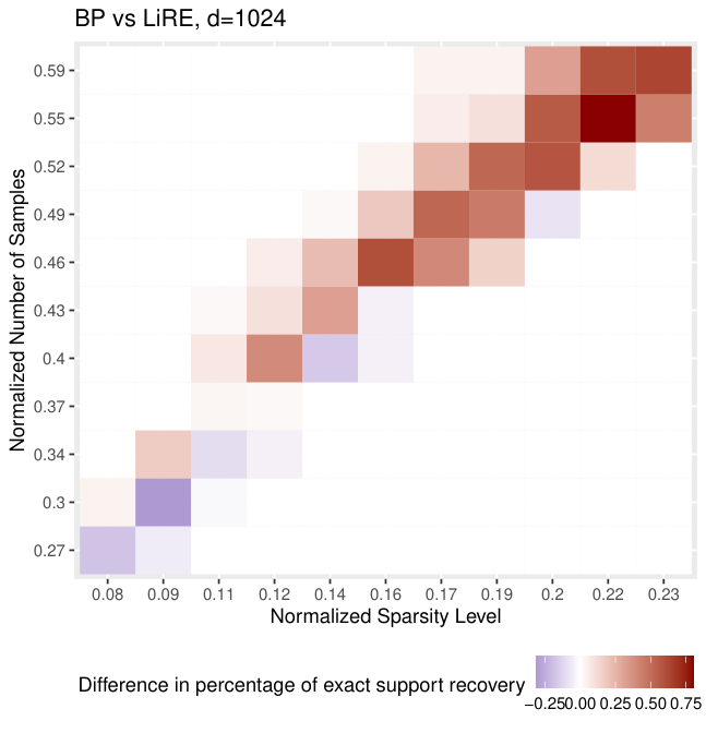
III-D LiRE as a standalone support recovery algorithm?

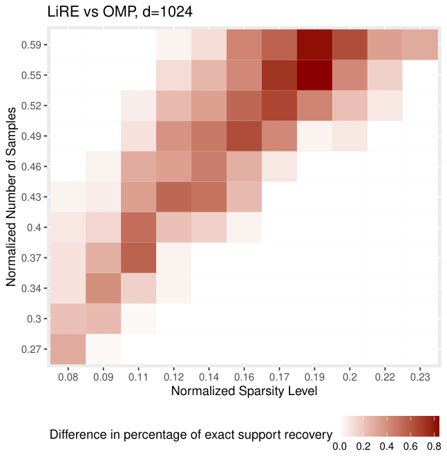
In the fourth set of experiments (Fig. 5), we compared LiRE (one pass) as a standalone support recovery algorithm against BP and OMP, and run similar experiments as described in Section III-B. LiRE was initialized with a randomly and uniformly selected 𝐬in\mathbf{s}_{\text{in}}. Fig. 5(a) gives the percentage of exact support recovery with BP minus the percentage of exact support recovery with LiRE. Red favors BP and blue favors LiRE, and similarly for LiRE against OMP in Fig. 5(b) where red favors LiRE. Recall that the computational complexities of LiRE and OMP are similar, of order 𝒪⁡(m​n​d){\cal{O}}(mnd), whereas it is order 𝒪⁡(n2​d1.5){\mathcal{O}}(n^{2}d^{1.5}) for BP.

Discussion

Fig. 5(a) shows that BP is superior to LiRE at higher sparsity levels. At lower sparsity levels performances appear to be close. Fig. 5(b) shows that LiRE achieves better performance than OMP, and that the difference gets more pronounced as the sparsity level increases.

Note here that with a random initialization 𝐬in\mathbf{s}_{\text{in}} may contain no correct feature, that is e¯=m\bar{e}=m. Applying Corollary 2 with the trivial upper bound e¯=m\bar{e}=m yields the sufficient condition

δ2​m+1≤12​m​(1+o⁡(1))m→∞\displaystyle\delta_{2m+1}\leq\frac{1}{\sqrt{2m}}(1+o(1))\quad m\to\infty (12)

for LiRE to recover an arbitrary number of errors. This condition is significantly more stringent than the sufficient condition for OMP to recover the underlying support: δm+1<1m+1\delta_{m+1}<\frac{1}{\sqrt{m+1}}. In light of Fig. 5(b), LiRE’s sufficient condition (12) to recover an arbitrary number of errors appears to be loose.

Refer to caption
(a) BP vs. LiRE.
Refer to caption
(b) LiRE vs. OMP.
Fig. 5: LiRE as a standalone support recovery algorithm. Red squares favor BP in Fig. 5(a) and favor LiRE in Fig. 5(b).

IV Analysis

Lemma 1 (Lemmas 11 and 22 in [12]).

Let 𝐥,𝐬\bm{l},\mathbf{s} be disjoint support vectors and suppose δ|𝐥|+|𝐬|<1\delta_{|\bm{l}|+|\mathbf{s}|}<1. Then, for all 𝐚∈ℝ|𝐥|\bf{a}\in\mathbb{R}^{|\bm{l}|} and 𝐛∈ℝ|𝐬|\bf{b}\in\mathbb{R}^{|\mathbf{s}|} we have

|𝐚𝖳​𝚽𝐥𝖳​𝚽𝐬​𝐛|≤δ|𝐥|+|𝐬|​‖𝐚‖𝟐​‖𝐛‖𝟐,\displaystyle|\bf{a}^{\mathsf{T}}{\mathbf{\Phi}}_{\bm{l}}^{\mathsf{T}}{\mathbf{\Phi}}_{\mathbf{s}}\bf{b}|\leq\delta_{|\bm{l}|+|\mathbf{s}|}||\bf{a}||_{2}||\bf{b}||_{2}\,,
‖𝚽𝒍𝖳​𝚽𝐬​𝐛‖𝟐≤δ|𝐥|+|𝐬|​‖𝐛‖𝟐.\displaystyle||{\mathbf{\Phi}}_{\bm{l}}^{\mathsf{T}}{\mathbf{\Phi}}_{\mathbf{s}}\bf{b}||_{2}\leq\delta_{|\bm{l}|+|\mathbf{s}|}||\bf{b}||_{2}\,.
Lemma 2.

Let 𝐬,𝐪\mathbf{s},\mathbf{q} be support vectors that are disjoint from support vector 𝐥\bm{l}. If max⁡{δ|𝐬|+|𝐥|,δ|𝐪|+|𝐥|}<1\max\{\delta_{|\mathbf{s}|+|\bm{l}|},\delta_{|\mathbf{q}|+|\bm{l}|}\}<1, then for any 𝐚∈ℝ|𝐬|{\bf{a}}\in\mathbb{R}^{|\mathbf{s}|} we have

‖P⁡{𝚽𝒍}​𝚽𝐬​𝐚‖2≤δ|𝐬|+|𝒍|1−δ|𝒍|​‖𝐚‖2,\displaystyle||P\{{\mathbf{\Phi}}_{\bm{l}}\}{\mathbf{\Phi}}_{\mathbf{s}}{\bf{a}}||_{2}\leq\frac{\delta_{|\mathbf{s}|+|\bm{l}|}}{\sqrt{1-\delta_{|\bm{l}|}}}||{\bf{a}}||_{2}\,,
‖𝚽𝐪𝖳​P​{𝚽𝒍}​𝚽𝐬​𝐚‖2≤δ|𝐬|+|𝒍|​δ|𝐪|+|𝒍|1−δ|𝒍|​‖𝐚‖𝟐.\displaystyle||{\mathbf{\Phi}}_{\mathbf{q}}^{\mathsf{T}}P\{{\mathbf{\Phi}}_{\bm{l}}\}{\mathbf{\Phi}}_{\mathbf{s}}{\bf{a}}||_{2}\leq\frac{\delta_{|\mathbf{s}|+|\bm{l}|}\delta_{|\mathbf{q}|+|\bm{l}|}}{{1-\delta_{|\bm{l}|}}}||\bf{a}||_{2}\,.
Proof.

We know that

‖P⁡{𝚽𝒍}​𝚽𝐬​𝐚‖22=𝐮𝖳​(𝚽𝒍𝖳​𝚽𝒍)−1​𝐮,||P\{{\mathbf{\Phi}}_{\bm{l}}\}{\mathbf{\Phi}}_{\mathbf{s}}{\bf{a}}||_{2}^{2}=\mathbf{u}^{\mathsf{T}}({\mathbf{\Phi}}^{\mathsf{T}}_{\bm{l}}{\mathbf{\Phi}}_{\bm{l}})^{-1}\mathbf{u}\,,

where 𝐮​=def​𝚽𝒍𝖳​𝚽𝐬​𝐚\mathbf{u}\overset{\text{def}}{=}{\mathbf{\Phi}}_{\bm{l}}^{\mathsf{T}}{\mathbf{\Phi}}_{\mathbf{s}}{\bf{a}}. From the definition of the restricted isometry property we get

𝐮𝖳​(𝚽𝒍𝖳​𝚽𝒍)−1​𝐮≤‖𝐮‖221−δ|𝒍|.\mathbf{u}^{\mathsf{T}}({\mathbf{\Phi}}^{\mathsf{T}}_{\bm{l}}{\mathbf{\Phi}}_{\bm{l}})^{-1}\mathbf{u}\leq\frac{||\mathbf{u}||_{2}^{2}}{1-\delta_{|\bm{l}|}}\,.

Next, Lemma 1 gives us

‖𝐮‖2≤δ|𝒍|+|𝐬|​‖𝐚‖2.||\mathbf{u}||_{2}\leq\delta_{|\bm{l}|+|\mathbf{s}|}||\mathbf{a}||_{2}\,.

This implies

‖P⁡{𝚽𝒍}​𝚽𝐬​a‖2≤δ|𝒍|+|𝐬|1−δ|𝒍|​‖a‖2.||P\{{\mathbf{\Phi}}_{\bm{l}}\}{\mathbf{\Phi}}_{\mathbf{s}}a||_{2}\leq\frac{\delta_{|\bm{l}|+|\mathbf{s}|}}{\sqrt{1-\delta_{|\bm{l}|}}}||a||_{2}.

For the proof of the second inequality in Lemma 2 first assume ‖𝐛‖2≤1||\mathbf{b}||_{2}\leq 1. Then, the Cauchy inequality yields

𝐛𝖳​𝚽𝐪𝖳​P​{𝚽𝒍}​𝚽𝐬​𝐚≤‖P⁡{𝚽𝒍}​𝚽𝐪​𝐛‖2||P⁡{𝚽𝒍}​𝚽𝐬​𝐚||2.\mathbf{b}^{\mathsf{T}}{\mathbf{\Phi}}_{\mathbf{q}}^{\mathsf{T}}P\{{\mathbf{\Phi}}_{\bm{l}}\}{\mathbf{\Phi}}_{\mathbf{s}}\mathbf{a}\leq||P\{{\mathbf{\Phi}}_{\bm{l}}\}{\mathbf{\Phi}}_{\mathbf{q}}\mathbf{b}||_{2}||P\{{\mathbf{\Phi}}_{\bm{l}}\}{\mathbf{\Phi}}_{\mathbf{s}}\mathbf{a}||_{2}.

Next, by invoking the first inequality in Lemma 2 we obtain

max‖𝐛‖2≤1⁡𝐛𝖳​𝚽𝐪𝖳​P​{𝚽𝒍}​𝚽𝐬​𝐚≤δ|𝐬|+|𝒍|​δ|𝐪|+|𝒍|1−δ|𝒍|​‖𝐚‖2,\max\limits_{||\mathbf{b}||_{2}\leq 1}\mathbf{b}^{\mathsf{T}}{\mathbf{\Phi}}_{\mathbf{q}}^{\mathsf{T}}P\{{\mathbf{\Phi}}_{\bm{l}}\}{\mathbf{\Phi}}_{\mathbf{s}}\mathbf{a}\leq\frac{\delta_{|\mathbf{s}|+|\bm{l}|}\delta_{|\mathbf{q}|+|\bm{l}|}}{{1-\delta_{|\bm{l}|}}}||\mathbf{a}||_{2}\,,

which establishes the desired result. ∎

Lemma 3.

Let 𝐬1,𝐬2\mathbf{s}_{1},\mathbf{s}_{2} be two disjoint support vectors with |𝐬1|=k1|\mathbf{s}_{1}|=k_{1} and |𝐬2|=k2|\mathbf{s}_{2}|=k_{2}. If δk1+k2≤0.5\delta_{k_{1}+k_{2}}\leq 0.5, then 𝚽𝐬1𝖳​(I−P⁡{𝚽𝐬2})​𝚽𝐬1{\mathbf{\Phi}}_{\mathbf{s}_{1}}^{\mathsf{T}}(I-P\{{\mathbf{\Phi}}_{\mathbf{s}_{2}}\}){\mathbf{\Phi}}_{\mathbf{s}_{1}} is invertible and

(𝚽𝐬1𝖳​(I−P⁡{𝚽𝐬2})​𝚽𝐬1)−1⪰11+δk1​Ik1.\displaystyle({\mathbf{\Phi}}_{\mathbf{s}_{1}}^{\mathsf{T}}(I-P\{{\mathbf{\Phi}}_{\mathbf{s}_{2}}\}){\mathbf{\Phi}}_{\mathbf{s}_{1}})^{-1}\succeq\frac{1}{1+\delta_{k_{1}}}I_{k_{1}}\,.
Proof.

Given 𝐳∈ℝk1{\mathbf{z}}\in\mathbb{R}^{k_{1}} we have

𝐳𝖳​(𝚽𝐬1𝖳​(I−P⁡{𝚽𝐬2})​𝚽𝐬1)​z=‖𝚽𝐬1​𝐳‖22−‖P⁡{𝚽𝐬2}​𝚽𝐬1​𝐳‖22,{\mathbf{z}}^{\mathsf{T}}({\mathbf{\Phi}}_{\mathbf{s}_{1}}^{\mathsf{T}}(I-P\{{\mathbf{\Phi}}_{\mathbf{s}_{2}}\}){\mathbf{\Phi}}_{\mathbf{s}_{1}})z=||{\mathbf{\Phi}}_{\mathbf{s}_{1}}{\mathbf{z}}||_{2}^{2}-||P\{{\mathbf{\Phi}}_{\mathbf{s}_{2}}\}{\mathbf{\Phi}}_{\mathbf{s}_{1}}{\mathbf{z}}||_{2}^{2}\,,

which is no larger than ‖𝚽𝐬1​𝐳‖22||{\mathbf{\Phi}}_{\mathbf{s}_{1}}{\mathbf{z}}||_{2}^{2}. Next, recall that the RIP property implies

‖𝚽𝐬1​z‖22≤(1+δk1)​‖𝐳‖22.||{\mathbf{\Phi}}_{\mathbf{s}_{1}}z||_{2}^{2}\leq(1+\delta_{k_{1}})||{\mathbf{z}}||_{2}^{2}. (13)

Therefore,

(𝚽𝐬1𝖳​(I−P⁡{𝚽𝐬2})​𝚽𝐬1)⪯(1+δk1)​Ik1.({\mathbf{\Phi}}_{\mathbf{s}_{1}}^{\mathsf{T}}(I-P\{{\mathbf{\Phi}}_{\mathbf{s}_{2}}\}){\mathbf{\Phi}}_{\mathbf{s}_{1}})\preceq(1+\delta_{k_{1}})I_{k_{1}}.

Moreover, Lemma 2 gives us

‖P⁡{𝚽𝐬2}​𝚽𝐬1​𝐳‖22≤δk2​‖𝐳‖221−δk2.||P\{{\mathbf{\Phi}}_{\mathbf{s}_{2}}\}{\mathbf{\Phi}}_{\mathbf{s}_{1}}{\mathbf{z}}||_{2}^{2}\leq\frac{\delta_{k}^{2}||{\mathbf{z}}||_{2}^{2}}{1-\delta_{k_{2}}}. (14)

By combining (13) and (14) we get

(1−δk1−δk21−δk2)​Ik1\displaystyle(1-\delta_{k_{1}}-\frac{\delta_{k}^{2}}{1-\delta_{k_{2}}})I_{k_{1}} ⪯(𝚽𝐬1𝖳​(I−P⁡{𝚽𝐬2})​𝚽𝐬1)\displaystyle\preceq({\mathbf{\Phi}}_{\mathbf{s}_{1}}^{\mathsf{T}}(I-P\{{\mathbf{\Phi}}_{\mathbf{s}_{2}}\}){\mathbf{\Phi}}_{\mathbf{s}_{1}})
⪯(1+δk1)​Ik1.\displaystyle\preceq(1+\delta_{k_{1}})I_{k_{1}}\,.

Therefore (𝚽𝐬1𝖳​(I−P⁡{𝚽𝐬2})​𝚽𝐬1)({\mathbf{\Phi}}_{\mathbf{s}_{1}}^{\mathsf{T}}(I-P\{{\mathbf{\Phi}}_{\mathbf{s}_{2}}\}){\mathbf{\Phi}}_{\mathbf{s}_{1}}) is invertible and we have the desired property. ∎

Lemma 4.

Let 𝐬1,𝐬2\mathbf{s}_{1},\mathbf{s}_{2} be two disjoint support vectors, let 𝐬=𝐬1∪𝐬2\mathbf{s}=\mathbf{s}_{1}\cup\mathbf{s}_{2}, and suppose δ|𝐬1|+|𝐬2|≤0.5\delta_{|\mathbf{s}_{1}|+|\mathbf{s}_{2}|}\leq 0.5. Then,

𝐱𝐬1=(𝚽𝐬1𝖳​(I−P⁡{𝚽𝐬2})​𝚽𝐬1)−1​𝚽𝐬1𝖳​𝐲⟂𝐬2.\displaystyle\mathbf{x}_{\mathbf{s}_{1}}=({\mathbf{\Phi}}_{\mathbf{s}_{1}}^{\mathsf{T}}(I-P\{{\mathbf{\Phi}}_{\mathbf{s}_{2}}\}){\mathbf{\Phi}}_{\mathbf{s}_{1}})^{-1}{\mathbf{\Phi}}_{\mathbf{s}_{1}}^{\mathsf{T}}{\mathbf{y}}^{\perp\mathbf{s}_{2}}.
Proof.

Since δ|𝐬1|+|𝐬2|<1\delta_{|\mathbf{s}_{1}|+|\mathbf{s}_{2}|}<1 we have that 𝚽𝐬{\mathbf{\Phi}}_{\mathbf{s}} is invertible and 𝐱𝐬=(𝚽𝐬𝖳​𝚽𝐬)−1​𝚽𝐬𝖳​𝐲{\mathbf{x}}_{\mathbf{s}}=({\mathbf{\Phi}}_{\mathbf{s}}^{\mathsf{T}}{\mathbf{\Phi}}_{\mathbf{s}})^{-1}{\mathbf{\Phi}}_{\mathbf{s}}^{\mathsf{T}}{\mathbf{y}}. Also, since 𝐬=𝐬1∪𝐬2\mathbf{s}=\mathbf{s}_{1}\cup\mathbf{s}_{2} we have

[𝐱𝐬1𝐱𝐬2]=[𝚽𝐬1𝖳​𝚽𝐬1𝚽𝐬1𝖳​𝚽𝐬2𝚽𝐬2𝖳​𝚽𝐬1𝚽𝐬2𝖳​𝚽𝐬2]−1​[𝚽𝐬1𝖳​𝐲𝚽𝐬2𝖳​𝐲].\displaystyle\begin{bmatrix}{\mathbf{x}}_{\mathbf{s}_{1}}\\ {\mathbf{x}}_{\mathbf{s}_{2}}\end{bmatrix}=\begin{bmatrix}{\mathbf{\Phi}}_{\mathbf{s}_{1}}^{\mathsf{T}}{\mathbf{\Phi}}_{\mathbf{s}_{1}}&{\mathbf{\Phi}}_{\mathbf{s}_{1}}^{\mathsf{T}}{\mathbf{\Phi}}_{\mathbf{s}_{2}}\\ {\mathbf{\Phi}}_{\mathbf{s}_{2}}^{\mathsf{T}}{\mathbf{\Phi}}_{\mathbf{s}_{1}}&{\mathbf{\Phi}}_{\mathbf{s}_{2}}^{\mathsf{T}}{\mathbf{\Phi}}_{\mathbf{s}_{2}}\\ \end{bmatrix}^{-1}\begin{bmatrix}{\mathbf{\Phi}}_{\mathbf{s}_{1}}^{\mathsf{T}}{\mathbf{y}}\\ {\mathbf{\Phi}}_{\mathbf{s}_{2}}^{\mathsf{T}}{\mathbf{y}}\\ \end{bmatrix}\,.

Let 𝚿{\mathbf{\Psi}} denote the Schur complement of block 𝚽𝐬2𝖳​𝚽𝐬2{\mathbf{\Phi}}_{\mathbf{s}_{2}}^{\mathsf{T}}{\mathbf{\Phi}}_{\mathbf{s}_{2}} of the matrix 𝚽𝐬𝖳​𝚽𝐬{\mathbf{\Phi}}_{\mathbf{s}}^{\mathsf{T}}{\mathbf{\Phi}}_{\mathbf{s}}. It then follows that

𝚿=𝚽𝐬1𝖳​𝚽𝐬1−𝚽𝐬1𝖳​𝚽𝐬2​(𝚽𝐬2𝖳​𝚽𝐬2)−1​𝚽𝐬2𝖳​𝚽𝐬1,{\mathbf{\Psi}}={\mathbf{\Phi}}_{\mathbf{s}_{1}}^{\mathsf{T}}{\mathbf{\Phi}}_{\mathbf{s}_{1}}-{\mathbf{\Phi}}_{\mathbf{s}_{1}}^{\mathsf{T}}{\mathbf{\Phi}}_{\mathbf{s}_{2}}({\mathbf{\Phi}}_{\mathbf{s}_{2}}^{\mathsf{T}}{\mathbf{\Phi}}_{\mathbf{s}_{2}})^{-1}{\mathbf{\Phi}}_{\mathbf{s}_{2}}^{\mathsf{T}}{\mathbf{\Phi}}_{\mathbf{s}_{1}},

i.e., 𝚿=𝚽𝐬1𝖳​(I−P⁡{𝚽𝐬2})​𝚽𝐬1{\mathbf{\Psi}}={\mathbf{\Phi}}_{\mathbf{s}_{1}}^{\mathsf{T}}(I-P\{{\mathbf{\Phi}}_{\mathbf{s}_{2}}\}){\mathbf{\Phi}}_{\mathbf{s}_{1}}. Since δ|𝐬1|+|𝐬2|≤0.5\delta_{|\mathbf{s}_{1}|+|\mathbf{s}_{2}|}\leq 0.5, we have that 𝚿{\mathbf{\Psi}} is invertible by Lemma 3. On the other hand, from the properties of invertible Schur complement we know that

𝐱𝐬1=𝚿−1​𝚽𝐬1𝖳​𝐲−𝚿−1​𝚽𝐬1𝖳​𝚽𝐬2​(𝚽𝐬2𝖳​𝚽𝐬2)−1​𝚽𝐬2𝖳​𝐲,{\mathbf{x}}_{\mathbf{s}_{1}}={\mathbf{\Psi}}^{-1}{\mathbf{\Phi}}_{\mathbf{s}_{1}}^{\mathsf{T}}{\mathbf{y}}-{\mathbf{\Psi}}^{-1}{\mathbf{\Phi}}_{\mathbf{s}_{1}}^{\mathsf{T}}{\mathbf{\Phi}}_{\mathbf{s}_{2}}({\mathbf{\Phi}}_{\mathbf{s}_{2}}^{\mathsf{T}}{\mathbf{\Phi}}_{\mathbf{s}_{2}})^{-1}{\mathbf{\Phi}}_{\mathbf{s}_{2}}^{\mathsf{T}}{\mathbf{y}},

which can be rewritten as 𝐱𝐬1=𝚿−1​𝚽𝐬1𝖳​𝐲⟂𝐬2{\mathbf{x}}_{\mathbf{s}_{1}}={\mathbf{\Psi}}^{-1}{\mathbf{\Phi}}_{\mathbf{s}_{1}}^{\mathsf{T}}{{\mathbf{y}}}^{\perp{\mathbf{s}_{2}}}, thereby completing the proof. ∎

Lemma 5.

Fix a length kk support vector 𝐥\bm{l}, let ℓ​=def​max⁡{m+1,k}\ell\overset{\text{def}}{=}\max\{m+1,k\}, and let 𝐱\mathbf{x} be the regression of 𝐲{\mathbf{y}} on 𝐥\bm{l}, i.e., 𝐱=ℰ⁡(𝐥)\mathbf{x}=\mathcal{E}(\bm{l}). If δℓ≤0.5\delta_{\ell}\leq 0.5, then for any 1≤j≤k1\leq j\leq k we have

|𝐱𝒍⁡[j]|≤δℓ1−δℓ−δℓ2​‖𝐱𝐬∗/𝒍∗‖2|\mathbf{x}_{\bm{l}[j]}|\leq\frac{\delta_{\ell}}{1-\delta_{\ell}-\delta_{\ell}^{2}}||\mathbf{x}^{*}_{\mathbf{s}^{*}/\bm{l}}||_{2}

whenever 𝐥⁡[j]∉𝐬∗\bm{l}[j]\notin\mathbf{s}^{*}.

Proof.

Write 𝒍\bm{l} as 𝒍⁡[j]∪𝒍⁡[−j]\bm{l}[j]\cup\bm{l}[-j]. Since δk≤0.5\delta_{k}\leq 0.5 we can apply Lemma 4 and get

|𝐱𝒍⁡[j]|=|𝚽𝒍⁡[j]𝖳​𝐲⟂𝒍⁡[−j]|‖𝚽𝒍⁡[j]⟂𝒍⁡[−j]‖22.|\mathbf{x}_{\bm{l}[j]}|=\frac{|{\mathbf{\Phi}}_{\bm{l}[j]}^{\mathsf{T}}{\mathbf{y}}^{\perp\bm{l}[-j]}|}{||{\mathbf{\Phi}}_{\bm{l}[j]}^{\perp\bm{l}[-j]}||_{2}^{2}}. (15)

We proceed by upper-bounding the numerator and lower-bounding the denominator of (15). For the numerator we have

|𝚽𝒍⁡[j]𝖳​𝐲⟂𝒍⁡[−j]|\displaystyle|{\mathbf{\Phi}}_{\bm{l}[j]}^{\mathsf{T}}{\mathbf{y}}^{\perp\bm{l}[-j]}| =|𝚽𝒍⁡[j]𝖳​(I−P⁡{𝚽𝒍⁡[−j]})​𝚽𝐬∗​𝐱∗|\displaystyle=|{\mathbf{\Phi}}_{\bm{l}[j]}^{\mathsf{T}}(I-P\{{\mathbf{\Phi}}_{\bm{l}[-j]}\}){\mathbf{\Phi}}_{\mathbf{s}^{*}}\mathbf{x}^{*}|
=|𝚽𝒍⁡[j]𝖳​(I−P⁡{𝚽𝒍⁡[−j]})​𝚽𝐬∗/𝒍⁡[−j]​𝐱𝐬∗/𝒍⁡[−j]∗|\displaystyle=|{\mathbf{\Phi}}_{\bm{l}[j]}^{\mathsf{T}}(I-P\{{\mathbf{\Phi}}_{\bm{l}[-j]}\}){\mathbf{\Phi}}_{\mathbf{s}^{*}/\bm{l}[-j]}\mathbf{x}^{*}_{\mathbf{s}^{*}/\bm{l}[-j]}|
≤|𝚽𝒍⁡[j]𝖳​𝚽𝐬∗/𝒍⁡[−j]​𝐱𝐬∗/𝒍⁡[−j]∗|+|𝚽𝒍⁡[j]𝖳​P​{𝚽𝒍⁡[−j]}​𝚽𝐬∗/𝒍⁡[−j]​𝐱𝐬∗/𝒍⁡[−j]∗|\displaystyle\leq|{\mathbf{\Phi}}_{\bm{l}[j]}^{\mathsf{T}}{\mathbf{\Phi}}_{\mathbf{s}^{*}/\bm{l}[-j]}\mathbf{x}^{*}_{\mathbf{s}^{*}/\bm{l}[-j]}|+|{\mathbf{\Phi}}_{\bm{l}[j]}^{\mathsf{T}}P\{{\mathbf{\Phi}}_{\bm{l}[-j]}\}{\mathbf{\Phi}}_{\mathbf{s}^{*}/\bm{l}[-j]}\mathbf{x}^{*}_{\mathbf{s}^{*}/\bm{l}[-j]}|
≤(a)​δm+1​‖𝐱𝐬∗/𝒍⁡[−j]∗‖2+‖P⁡{𝚽𝒍⁡[−j]}​𝚽𝒍⁡[j]‖2||P⁡{𝚽𝒍⁡[−j]}​𝚽𝐬∗/𝒍⁡[−j]​𝐱𝐬∗/𝒍⁡[−j]∗||2\displaystyle\overset{(a)}{\leq}\delta_{m+1}||\mathbf{x}^{*}_{\mathbf{s}^{*}/\bm{l}[-j]}||_{2}+||P\{{\mathbf{\Phi}}_{\bm{l}[-j]}\}{\mathbf{\Phi}}_{\bm{l}[j]}||_{2}||P\{{\mathbf{\Phi}}_{\bm{l}[-j]}\}{\mathbf{\Phi}}_{\mathbf{s}^{*}/\bm{l}[-j]}\mathbf{x}^{*}_{\mathbf{s}^{*}/\bm{l}[-j]}||_{2}
≤(b)​δm+1​‖𝐱𝐬∗/𝒍⁡[−j]∗‖2+δk21−δk−1​‖𝐱𝐬∗/𝒍⁡[−j]∗‖2,\displaystyle\overset{(b)}{\leq}\delta_{m+1}||\mathbf{x}^{*}_{\mathbf{s}^{*}/\bm{l}[-j]}||_{2}+\frac{\delta_{k}^{2}}{1-\delta_{k-1}}||\mathbf{x}^{*}_{\mathbf{s}^{*}/\bm{l}[-j]}||_{2}\,,

where (a)(a) follows from Lemma 1 and where (b)(b) holds by Lemma 2 and the Cauchy inequality. Therefore, from the monotonicity of the RIP constant we get

|𝚽𝒍⁡[j]𝖳​𝐲⟂𝒍⁡[−j]|≤δℓ1−δℓ​‖𝐱𝐬∗/𝒍⁡[−j]∗‖2.|{\mathbf{\Phi}}_{\bm{l}[j]}^{\mathsf{T}}{\mathbf{y}}^{\perp\bm{l}[-j]}|\leq\frac{\delta_{\ell}}{1-\delta_{\ell}}||\mathbf{x}^{*}_{\mathbf{s}^{*}/\bm{l}[-j]}||_{2}. (16)

For the denominator of (15) we have

‖𝚽𝒍⁡[j]⟂𝒍⁡[−j]‖22=1−‖P⁡{𝚽𝒍⁡[−j]}​𝚽𝒍⁡[j]‖22,||{\mathbf{\Phi}}_{\bm{l}[j]}^{\perp\bm{l}[-j]}||_{2}^{2}=1-||P\{{\mathbf{\Phi}}_{\bm{l}[-j]}\}{\mathbf{\Phi}}_{\bm{l}[j]}||_{2}^{2},

hence by Lemma 2 we get ‖𝚽𝒍⁡[j]⟂𝒍⁡[−j]‖22≥1−δk21−δk−1||{\mathbf{\Phi}}_{\bm{l}[j]}^{\perp\bm{l}[-j]}||_{2}^{2}\geq 1-\frac{\delta^{2}_{k}}{1-\delta_{k-1}}. This inequality together with inequalities (16) and (15) complete the proof. ∎

Lemma 6.

Let 𝐬\mathbf{s} be a support vector of size kk, and e=|𝐬∗\𝐬|e=|\mathbf{s}^{*}\backslash\mathbf{s}|. Under setting (1), suppose k+ℓ>mk+\ell>m, ℓ≤e\ell\leq e, and suppose the design matrix 𝚽{\mathbf{\Phi}} satisfies δk+ℓ≤0.5\delta_{k+\ell}\leq 0.5. Let 𝐥​=def​ℒ​(ℓ,𝐬)\bm{l}\overset{\text{def}}{=}{\mathcal{L}}(\ell,\mathbf{s}), 𝐱​=def​ℰ​(𝐩){\mathbf{x}}\overset{\text{def}}{=}\mathcal{E}(\mathbf{p}), and t​=def​max⁡{k+e,ℓ+e}t\overset{\text{def}}{=}\max\{k+e,\ell+e\}. Consider j∈𝐥j\in\bm{l} such that |𝐱^j|=‖𝐱^𝐥‖∞|\hat{\mathbf{x}}_{j}|=||\hat{\mathbf{x}}_{\bm{l}}||_{\infty}. If 𝐬∗⊄𝐩\mathbf{s}^{*}\not\subset\mathbf{p} and j∉𝐬∗j\notin\mathbf{s}^{*}, then

‖𝐱𝒍∩𝐬∗∗‖2≤(δt​(1−δt2)​2​e(1−δt−δt2)​(1−2​δt)−1)​‖𝐱𝐬∗\𝐩∗‖2.||\mathbf{x}^{*}_{\bm{l}\cap\mathbf{s}^{*}}||_{2}\leq\left(\frac{\delta_{t}(1-\delta^{2}_{t})\sqrt{2e}}{(1-\delta_{t}-\delta_{t}^{2})(1-2\delta_{t})}-1\right)||\mathbf{x}^{*}_{\mathbf{s}^{*}\backslash\mathbf{p}}||_{2}.
Proof.

From Lemma 5 we have

|𝐱^j|≤δk+ℓ1−δk+ℓ−δk+ℓ2​‖𝐱𝐬∗\𝐩∗‖2.|\hat{\mathbf{x}}_{j}|\leq\frac{\delta_{k+\ell}}{1-\delta_{k+\ell}-\delta_{k+\ell}^{2}}||\mathbf{x}^{*}_{\mathbf{s}^{*}\backslash\mathbf{p}}||_{2}. (17)

On the other hand, we have

‖𝐱^𝒍‖∞\displaystyle||\hat{\mathbf{x}}_{\bm{l}}||_{\infty} =‖(𝚽𝒍𝖳​(I−P⁡{𝚽𝐬})​𝚽𝒍)−1​𝚽𝒍𝖳​𝐲⟂𝐬‖∞\displaystyle=||({\mathbf{\Phi}}_{\bm{l}}^{\mathsf{T}}(I-P\{{\mathbf{\Phi}}_{\mathbf{s}}\}){\mathbf{\Phi}}_{\bm{l}})^{-1}{\mathbf{\Phi}}_{\bm{l}}^{\mathsf{T}}{\mathbf{y}}^{\perp\mathbf{s}}||_{\infty}
≥1ℓ​‖(𝚽𝒍𝖳​(I−P⁡{𝚽𝐬})​𝚽𝒍)−1​𝚽𝒍𝖳​𝐲⟂𝐬‖2\displaystyle\geq\frac{1}{\sqrt{\ell}}||({\mathbf{\Phi}}_{\bm{l}}^{\mathsf{T}}(I-P\{{\mathbf{\Phi}}_{\mathbf{s}}\}){\mathbf{\Phi}}_{\bm{l}})^{-1}{\mathbf{\Phi}}_{\bm{l}}^{\mathsf{T}}{\mathbf{y}}^{\perp\mathbf{s}}||_{2}
≥(a)​1ℓ​(1+δℓ)​‖𝚽𝒍𝖳​𝐲⟂𝐬‖2\displaystyle\overset{(a)}{\geq}\frac{1}{\sqrt{\ell}(1+\delta_{\ell})}||{\mathbf{\Phi}}_{\bm{l}}^{\mathsf{T}}{\mathbf{y}}^{\perp\mathbf{s}}||_{2}
≥(b)​1e​(1+δℓ)​‖𝚽𝐬∗\𝐬𝖳​𝐲⟂𝐬‖2\displaystyle\overset{(b)}{\geq}\frac{1}{\sqrt{e}(1+\delta_{\ell})}||{\mathbf{\Phi}}_{\mathbf{s}^{*}\backslash\mathbf{s}}^{\mathsf{T}}{\mathbf{y}}^{\perp\mathbf{s}}||_{2}
≥(c)​1e​(1+δℓ)​(‖𝚽𝐬∗\𝐬𝖳​𝚽𝐬∗\𝐬​𝐱𝐬∗\𝐬∗‖2−CLOSE\displaystyle\overset{(c)}{\geq}\frac{1}{\sqrt{e}(1+\delta_{\ell})}\big(||{\mathbf{\Phi}}_{\mathbf{s}^{*}\backslash\mathbf{s}}^{\mathsf{T}}{\mathbf{\Phi}}_{\mathbf{s}^{*}\backslash\mathbf{s}}\mathbf{x}^{*}_{\mathbf{s}^{*}\backslash\mathbf{s}}||_{2}-
OPEN‖𝚽𝐬∗\𝐬𝖳​P​{𝚽𝐬}​𝚽𝐬∗\𝐬​𝐱𝐬∗\𝐬∗‖2)\displaystyle||{\mathbf{\Phi}}_{\mathbf{s}^{*}\backslash\mathbf{s}}^{\mathsf{T}}P\{{\mathbf{\Phi}}_{\mathbf{s}}\}{\mathbf{\Phi}}_{\mathbf{s}^{*}\backslash\mathbf{s}}\mathbf{x}^{*}_{\mathbf{s}^{*}\backslash\mathbf{s}}||_{2}\big)
≥(d)​1e​(1+δℓ)​((1−δe)​‖𝐱𝐬∗\𝐬∗‖2−δk+e21−δk​‖𝐱𝐬∗\𝐬∗‖2),\displaystyle\overset{(d)}{\geq}\frac{1}{\sqrt{e}(1+\delta_{\ell})}\left((1-\delta_{e})||\mathbf{x}^{*}_{\mathbf{s}^{*}\backslash\mathbf{s}}||_{2}-\frac{\delta^{2}_{k+e}}{1-\delta_{k}}||\mathbf{x}^{*}_{\mathbf{s}^{*}\backslash\mathbf{s}}||_{2}\right)\,,

where (a)(a) follows from Lemma 3; where (b)(b) is a direct result from the definition of 𝒍\bm{l} along with the fact that 𝐬∗\𝐩\mathbf{s}^{*}\backslash\mathbf{p} is non-empty and |𝒍|≤e|\bm{l}|\leq e; where (c)(c) follows from definition of 𝐲⟂𝐬{{\mathbf{y}}}^{\perp{\mathbf{s}}} and the triangle inequality; and where (d)(d) follows from the RIP definition together with Lemma 2. Next, by combining the above inequality with (17) and using the monotonicity of the RIP constant, we deduce that if j∉𝐬∗j\notin\mathbf{s}^{*}, then

δt1−δt−δt2​‖𝐱𝐬∗\𝐩∗‖2≥(1−2​δt)e​(1−δt2)​‖𝐱𝐬∗\𝐬∗‖2.\frac{\delta_{t}}{1-\delta_{t}-\delta_{t}^{2}}||\mathbf{x}^{*}_{\mathbf{s}^{*}\backslash\mathbf{p}}||_{2}\geq\frac{(1-2\delta_{t})}{\sqrt{e}(1-\delta_{t}^{2})}||\mathbf{x}^{*}_{\mathbf{s}^{*}\backslash\mathbf{s}}||_{2}\,.

This implies

‖𝐱𝐬∗\𝐬∗‖2≤δt​(1−δt2)​e(1−δt−δt2)​(1−2​δt)​‖𝐱𝐬∗\𝐩∗‖2.||\mathbf{x}^{*}_{\mathbf{s}^{*}\backslash\mathbf{s}}||_{2}\leq\frac{\delta_{t}(1-\delta^{2}_{t})\sqrt{e}}{(1-\delta_{t}-\delta_{t}^{2})(1-2\delta_{t})}||\mathbf{x}^{*}_{\mathbf{s}^{*}\backslash\mathbf{p}}||_{2}. (18)

Now, since 𝐬∗\𝐬=(𝒍∩𝐬∗)∪(𝐬∗\𝐩)\mathbf{s}^{*}\backslash\mathbf{s}=(\bm{l}\cap\mathbf{s}^{*})\cup(\mathbf{s}^{*}\backslash\mathbf{p}), we have 2​‖𝐱𝐬∗\𝐬∗‖2≥‖𝐱𝒍∩𝐬∗∗‖2+||𝐱𝐬∗\𝐩∗||2\sqrt{2}||\mathbf{x}^{*}_{\mathbf{s}^{*}\backslash\mathbf{s}}||_{2}\geq||\mathbf{x}^{*}_{\bm{l}\cap\mathbf{s}^{*}}||_{2}+||\mathbf{x}^{*}_{\mathbf{s}^{*}\backslash\mathbf{p}}||_{2}. Using this inequality in (18) completes the proof. ∎

Lemma 7.

Let 𝐬\mathbf{s} be a support vector of size kk. Let 𝐥​=def​ℒ​(ℓ,𝐬)\bm{l}\overset{\text{def}}{=}{\mathcal{L}}(\ell,\mathbf{s}), 𝐩​=def​𝐬∪𝐥\mathbf{p}\overset{\text{def}}{=}\mathbf{s}\cup\bm{l}, e​=def​|𝐬∗\𝐬|e\overset{\text{def}}{=}|\mathbf{s}^{*}\backslash\mathbf{s}|, and t​=def​max⁡{k+e,e+ℓ}t\overset{\text{def}}{=}\max\{k+e,e+\ell\}. If 𝐬∗⊄𝐩\mathbf{s}^{*}\not\subset\mathbf{p}, then

(1+δt−δt21−δt)||𝐱𝒍∩𝐬∗∗||2+(2​δt−δt21−δk)​‖𝐱𝐬∗\𝐩∗‖2≥(1−2​δt1−δt​‖𝐱𝐬∗\𝐩∗‖2−δt1−δt||𝐱𝐬∗∩𝒍∗||2)⋅ℓ|𝐬∗\𝐩|\displaystyle\left(\frac{1+\delta_{t}-\delta_{t}^{2}}{1-\delta_{t}}\right)||\mathbf{x}^{*}_{\bm{l}\cap\mathbf{s}^{*}}||_{2}+\left(\frac{2\delta_{t}-\delta_{t}^{2}}{1-\delta_{k}}\right)||\mathbf{x}^{*}_{\mathbf{s}^{*}\backslash\mathbf{p}}||_{2}\geq\Big(\frac{1-2\delta_{t}}{1-\delta_{t}}||\mathbf{x}^{*}_{\mathbf{s}^{*}\backslash\mathbf{p}}||_{2}-\frac{\delta_{t}}{1-\delta_{t}}||\mathbf{x}^{*}_{\mathbf{s}^{*}\cap\bm{l}}||_{2}\Big)\cdot\sqrt{\frac{\ell}{{|\mathbf{s}^{*}\backslash\mathbf{p}|}}}
Proof of Lemma 7.

From the definition of ℒ⁡(ℓ,𝐬){\mathcal{L}}(\ell,\mathbf{s}) and the fact that 𝐬∗\𝐩\mathbf{s}^{*}\backslash\mathbf{p} is non-empty, we have ‖𝚽𝒍𝖳​𝐲⟂𝐬‖2ℓ≥‖𝚽𝐬∗\𝐩𝖳​𝐲⟂𝐬‖∞\frac{||{\mathbf{\Phi}}_{\bm{l}}^{\mathsf{T}}{{\mathbf{y}}}^{\perp{\mathbf{s}}}||_{2}}{\sqrt{\ell}}\geq||{\mathbf{\Phi}}_{\mathbf{s}^{*}\backslash\mathbf{p}}^{\mathsf{T}}{{\mathbf{y}}}^{\perp{\mathbf{s}}}||_{\infty}. Then, since ‖𝚽𝐬∗\𝐩𝖳​𝐲⟂𝐬‖∞≥‖𝚽𝐬∗\𝐩𝖳​𝐲⟂𝐬‖2|𝐬∗\𝐩|,||{\mathbf{\Phi}}_{\mathbf{s}^{*}\backslash\mathbf{p}}^{\mathsf{T}}{{\mathbf{y}}}^{\perp{\mathbf{s}}}||_{\infty}\geq\frac{||{\mathbf{\Phi}}_{\mathbf{s}^{*}\backslash\mathbf{p}}^{\mathsf{T}}{{\mathbf{y}}}^{\perp{\mathbf{s}}}||_{2}}{\sqrt{|\mathbf{s}^{*}\backslash\mathbf{p}|}}, we get

‖𝚽𝒍𝖳​𝐲⟂𝐬‖2≥ℓ|𝐬∗\𝐩|​‖𝚽𝐬∗\𝐩𝖳​𝐲⟂𝐬‖2.||{\mathbf{\Phi}}_{\bm{l}}^{\mathsf{T}}{{\mathbf{y}}}^{\perp{\mathbf{s}}}||_{2}\geq\sqrt{\frac{\ell}{{|\mathbf{s}^{*}\backslash\mathbf{p}|}}}||{\mathbf{\Phi}}_{\mathbf{s}^{*}\backslash\mathbf{p}}^{\mathsf{T}}{{\mathbf{y}}}^{\perp{\mathbf{s}}}||_{2}. (19)

Now, on the hand we have

‖𝚽𝐬∗\𝐩𝖳​𝐲⟂𝐬‖2\displaystyle||{\mathbf{\Phi}}_{\mathbf{s}^{*}\backslash\mathbf{p}}^{\mathsf{T}}{{\mathbf{y}}}^{\perp{\mathbf{s}}}||_{2} =‖𝚽𝐬∗\𝐩𝖳​(I−P⁡{𝚽𝐬})​𝚽𝐬∗\𝐬​𝐱𝐬∗\𝐬∗‖2\displaystyle=||{\mathbf{\Phi}}_{\mathbf{s}^{*}\backslash\mathbf{p}}^{\mathsf{T}}(I-P\{{\mathbf{\Phi}}_{\mathbf{s}}\}){\mathbf{\Phi}}_{\mathbf{s}^{*}\backslash\mathbf{s}}\mathbf{x}^{*}_{\mathbf{s}^{*}\backslash\mathbf{s}}||_{2}
≥‖𝚽𝐬∗\𝐩𝖳​𝚽𝐬∗\𝐬​𝐱𝐬∗\𝐬∗‖2−‖𝚽𝐬∗\𝐩𝖳​P​{𝚽𝐬}​𝚽𝐬∗\𝐬​𝐱𝐬∗\𝐬∗‖2\displaystyle\geq||{\mathbf{\Phi}}_{\mathbf{s}^{*}\backslash\mathbf{p}}^{\mathsf{T}}{\mathbf{\Phi}}_{\mathbf{s}^{*}\backslash\mathbf{s}}\mathbf{x}^{*}_{\mathbf{s}^{*}\backslash\mathbf{s}}||_{2}-||{\mathbf{\Phi}}_{\mathbf{s}^{*}\backslash\mathbf{p}}^{\mathsf{T}}P\{{\mathbf{\Phi}}_{\mathbf{s}}\}{\mathbf{\Phi}}_{\mathbf{s}^{*}\backslash\mathbf{s}}\mathbf{x}^{*}_{\mathbf{s}^{*}\backslash\mathbf{s}}||_{2}
≥(a)​‖𝚽𝐬∗\𝐩𝖳​𝚽𝐬∗\𝐬​𝐱𝐬∗\𝐬∗‖2−δk+e21−δk​‖𝐱𝐬∗\𝐬∗‖2\displaystyle\overset{(a)}{\geq}||{\mathbf{\Phi}}_{\mathbf{s}^{*}\backslash\mathbf{p}}^{\mathsf{T}}{\mathbf{\Phi}}_{\mathbf{s}^{*}\backslash\mathbf{s}}\mathbf{x}^{*}_{\mathbf{s}^{*}\backslash\mathbf{s}}||_{2}-\frac{\delta_{k+e}^{2}}{1-\delta_{k}}||\mathbf{x}^{*}_{\mathbf{s}^{*}\backslash\mathbf{s}}||_{2}
≥(b)​‖𝚽𝐬∗\𝐩𝖳​𝚽𝐬∗\𝐩​𝐱𝐬∗\𝐩∗‖2−‖𝚽𝐬∗\𝐩𝖳​𝚽𝐬∗∩𝒍​𝐱𝐬∗∩𝒍∗‖2−δk+e21−δk||𝐱𝐬∗\𝐬∗||2\displaystyle\overset{(b)}{\geq}||{\mathbf{\Phi}}_{\mathbf{s}^{*}\backslash\mathbf{p}}^{\mathsf{T}}{\mathbf{\Phi}}_{\mathbf{s}^{*}\backslash\mathbf{p}}\mathbf{x}^{*}_{\mathbf{s}^{*}\backslash\mathbf{p}}||_{2}-||{\mathbf{\Phi}}_{\mathbf{s}^{*}\backslash\mathbf{p}}^{\mathsf{T}}{\mathbf{\Phi}}_{\mathbf{s}^{*}\cap\bm{l}}\mathbf{x}^{*}_{\mathbf{s}^{*}\cap\bm{l}}||_{2}-\frac{\delta^{2}_{k+e}}{1-\delta_{k}}||\mathbf{x}^{*}_{\mathbf{s}^{*}\backslash\mathbf{s}}||_{2}
≥(c)​‖𝚽𝐬∗\𝐩𝖳​𝚽𝐬∗\𝐩​𝐱𝐬∗\𝐩∗‖2−δe​‖𝐱𝐬∗∩𝒍∗‖2−δk+e21−δk||𝐱𝐬∗\𝐬∗||2\displaystyle\overset{(c)}{\geq}||{\mathbf{\Phi}}_{\mathbf{s}^{*}\backslash\mathbf{p}}^{\mathsf{T}}{\mathbf{\Phi}}_{\mathbf{s}^{*}\backslash\mathbf{p}}\mathbf{x}^{*}_{\mathbf{s}^{*}\backslash\mathbf{p}}||_{2}-\delta_{e}||\mathbf{x}^{*}_{\mathbf{s}^{*}\cap\bm{l}}||_{2}-\frac{\delta^{2}_{k+e}}{1-\delta_{k}}||\mathbf{x}^{*}_{\mathbf{s}^{*}\backslash\mathbf{s}}||_{2}
≥(d)​(1−δ|𝐬∗\𝐩|)​‖𝐱𝐬∗\𝐩∗‖2−δe​‖𝐱𝐬∗∩𝒍∗‖2−δk+e21−δk||𝐱𝐬∗\𝐬∗||2\displaystyle\overset{(d)}{\geq}(1-\delta_{|\mathbf{s}^{*}\backslash\mathbf{p}|})||\mathbf{x}^{*}_{\mathbf{s}^{*}\backslash\mathbf{p}}||_{2}-\delta_{e}||\mathbf{x}^{*}_{\mathbf{s}^{*}\cap\bm{l}}||_{2}-\frac{\delta^{2}_{k+e}}{1-\delta_{k}}||\mathbf{x}^{*}_{\mathbf{s}^{*}\backslash\mathbf{s}}||_{2}
≥(e)​(1−δe)​‖𝐱𝐬∗\𝐩∗‖2−δe​‖𝐱𝐬∗∩𝒍∗‖2−δk+e21−δk||𝐱𝐬∗\𝐬∗||2\displaystyle\overset{(e)}{\geq}(1-\delta_{e})||\mathbf{x}^{*}_{\mathbf{s}^{*}\backslash\mathbf{p}}||_{2}-\delta_{e}||\mathbf{x}^{*}_{\mathbf{s}^{*}\cap\bm{l}}||_{2}-\frac{\delta^{2}_{k+e}}{1-\delta_{k}}||\mathbf{x}^{*}_{\mathbf{s}^{*}\backslash\mathbf{s}}||_{2}
≥(b)​(1−δe−δk+e21−δk)​‖𝐱𝐬∗\𝐩∗‖2−(δe+δk+e21−δk)​‖𝐱𝐬∗∩𝒍∗‖2,\displaystyle\overset{(b)}{\geq}(1-\delta_{e}-\frac{\delta^{2}_{k+e}}{1-\delta_{k}})||\mathbf{x}^{*}_{\mathbf{s}^{*}\backslash\mathbf{p}}||_{2}-(\delta_{e}+\frac{\delta_{k+e}^{2}}{1-\delta_{k}})||\mathbf{x}^{*}_{\mathbf{s}^{*}\cap\bm{l}}||_{2}\,, (20)

where (a)(a) holds by Lemma 2; where (b)(b) follows from the triangle inequality and the identity 𝐬∗\𝐬=(𝐬∗∩𝒍)∪(𝐬∗\𝐩)\mathbf{s}^{*}\backslash\mathbf{s}=(\mathbf{s}^{*}\cap\bm{l})\cup(\mathbf{s}^{*}\backslash\mathbf{p}); where (c)(c) is a direct result of Lemma 1; where (d)(d) follows from the definition of RIP constant; and where (e)(e) holds by the monotonicity of the RIP constant and the fact that |𝐬∗\𝐩|≤e|\mathbf{s}^{*}\backslash\mathbf{p}|\leq e.

On the other hand, we have

‖𝚽𝒍𝖳​𝐲⟂𝐬‖2\displaystyle||{\mathbf{\Phi}}_{\bm{l}}^{\mathsf{T}}{{\mathbf{y}}}^{\perp{\mathbf{s}}}||_{2} =‖𝚽𝒍𝖳​(I−P⁡{𝚽𝐬})​𝚽𝐬∗​𝐱𝐬∗∗‖2\displaystyle=||{\mathbf{\Phi}}_{\bm{l}}^{\mathsf{T}}(I-P\{{\mathbf{\Phi}}_{\mathbf{s}}\}){\mathbf{\Phi}}_{\mathbf{s}^{*}}\mathbf{x}^{*}_{\mathbf{s}^{*}}||_{2}
=‖𝚽𝒍𝖳​(I−P⁡{𝚽𝐬})​𝚽𝐬∗\𝐬​𝐱𝐬∗\𝐬∗‖2\displaystyle=||{\mathbf{\Phi}}_{\bm{l}}^{\mathsf{T}}(I-P\{{\mathbf{\Phi}}_{\mathbf{s}}\}){\mathbf{\Phi}}_{\mathbf{s}^{*}\backslash\mathbf{s}}\mathbf{x}^{*}_{\mathbf{s}^{*}\backslash\mathbf{s}}||_{2}
≤‖𝚽𝒍𝖳​𝚽𝐬∗\𝐬​𝐱𝐬∗\𝐬∗‖2+‖𝚽𝒍𝖳​P​{𝚽𝐬}​𝚽𝐬∗\𝐬​𝐱𝐬∗\𝐬∗‖2\displaystyle\leq||{\mathbf{\Phi}}_{\bm{l}}^{\mathsf{T}}{\mathbf{\Phi}}_{\mathbf{s}^{*}\backslash\mathbf{s}}\mathbf{x}^{*}_{\mathbf{s}^{*}\backslash\mathbf{s}}||_{2}+||{\mathbf{\Phi}}_{\bm{l}}^{\mathsf{T}}P\{{\mathbf{\Phi}}_{\mathbf{s}}\}{\mathbf{\Phi}}_{\mathbf{s}^{*}\backslash\mathbf{s}}\mathbf{x}^{*}_{\mathbf{s}^{*}\backslash\mathbf{s}}||_{2}
≤(a)​‖𝚽𝒍𝖳​𝚽𝐬∗\𝐬​𝐱𝐬∗\𝐬∗‖2+δe+k​δk+ℓ1−δk​‖𝐱𝐬∗\𝐬∗‖2\displaystyle\overset{(a)}{\leq}||{\mathbf{\Phi}}_{\bm{l}}^{\mathsf{T}}{\mathbf{\Phi}}_{\mathbf{s}^{*}\backslash\mathbf{s}}\mathbf{x}^{*}_{\mathbf{s}^{*}\backslash\mathbf{s}}||_{2}+\frac{\delta_{e+k}\delta_{k+\ell}}{1-\delta_{k}}||\mathbf{x}^{*}_{\mathbf{s}^{*}\backslash\mathbf{s}}||_{2}
≤(b)​‖𝚽𝒍\𝐬∗𝖳​𝚽𝐬∗\𝐬​𝐱𝐬∗\𝐬∗‖2+‖𝚽𝒍∩𝐬∗𝖳​𝚽𝐬∗\𝐬​𝐱𝐬∗\𝐬∗‖2+δe+k​δk+ℓ1−δk||𝐱𝐬∗\𝐬∗||2\displaystyle\overset{(b)}{\leq}||{\mathbf{\Phi}}_{\bm{l}\backslash\mathbf{s}^{*}}^{\mathsf{T}}{\mathbf{\Phi}}_{\mathbf{s}^{*}\backslash\mathbf{s}}\mathbf{x}^{*}_{\mathbf{s}^{*}\backslash\mathbf{s}}||_{2}+||{\mathbf{\Phi}}_{\bm{l}\cap\mathbf{s}^{*}}^{\mathsf{T}}{\mathbf{\Phi}}_{\mathbf{s}^{*}\backslash\mathbf{s}}\mathbf{x}^{*}_{\mathbf{s}^{*}\backslash\mathbf{s}}||_{2}+\frac{\delta_{e+k}\delta_{k+\ell}}{1-\delta_{k}}||\mathbf{x}^{*}_{\mathbf{s}^{*}\backslash\mathbf{s}}||_{2}
≤(c)​(δℓ+e+δe+k​δk+ℓ1−δk)​‖𝐱𝐬∗\𝐬∗‖2+‖𝚽𝒍∩𝐬∗𝖳​𝚽𝐬∗\𝐬​𝐱𝐬∗\𝐬∗‖2\displaystyle\overset{(c)}{\leq}(\delta_{\ell+e}+\frac{\delta_{e+k}\delta_{k+\ell}}{1-\delta_{k}})||\mathbf{x}^{*}_{\mathbf{s}^{*}\backslash\mathbf{s}}||_{2}+||{\mathbf{\Phi}}_{\bm{l}\cap\mathbf{s}^{*}}^{\mathsf{T}}{\mathbf{\Phi}}_{\mathbf{s}^{*}\backslash\mathbf{s}}\mathbf{x}^{*}_{\mathbf{s}^{*}\backslash\mathbf{s}}||_{2}
≤(d)​(δℓ+e+δe+k​δk+ℓ1−δk)​‖𝐱𝐬∗\𝐬∗‖2+‖𝚽𝒍∩𝐬∗𝖳​𝚽𝒍∩𝐬∗​𝐱𝒍∩𝐬∗∗‖2+||𝚽𝒍∩𝐬∗𝖳​𝚽𝐬∗\𝐩​𝐱𝐬∗\𝐩∗||2\displaystyle\overset{(d)}{\leq}(\delta_{\ell+e}+\frac{\delta_{e+k}\delta_{k+\ell}}{1-\delta_{k}})||\mathbf{x}^{*}_{\mathbf{s}^{*}\backslash\mathbf{s}}||_{2}+||{\mathbf{\Phi}}_{\bm{l}\cap\mathbf{s}^{*}}^{\mathsf{T}}{\mathbf{\Phi}}_{\bm{l}\cap\mathbf{s}^{*}}\mathbf{x}^{*}_{\bm{l}\cap\mathbf{s}^{*}}||_{2}+||{\mathbf{\Phi}}_{\bm{l}\cap\mathbf{s}^{*}}^{\mathsf{T}}{\mathbf{\Phi}}_{\mathbf{s}^{*}\backslash\mathbf{p}}\mathbf{x}^{*}_{\mathbf{s}^{*}\backslash\mathbf{p}}||_{2}
≤(e)​(δℓ+e+δe+k​δk+ℓ1−δk)​‖𝐱𝐬∗\𝐬∗‖2+(1+δe)​‖𝐱𝒍∩𝐬∗∗‖2+||𝚽𝒍∩𝐬∗𝖳​𝚽𝐬∗\𝐩​𝐱𝐬∗\𝐩∗||2\displaystyle\overset{(e)}{\leq}(\delta_{\ell+e}+\frac{\delta_{e+k}\delta_{k+\ell}}{1-\delta_{k}})||\mathbf{x}^{*}_{\mathbf{s}^{*}\backslash\mathbf{s}}||_{2}+(1+\delta_{e})||\mathbf{x}^{*}_{\bm{l}\cap\mathbf{s}^{*}}||_{2}+||{\mathbf{\Phi}}_{\bm{l}\cap\mathbf{s}^{*}}^{\mathsf{T}}{\mathbf{\Phi}}_{\mathbf{s}^{*}\backslash\mathbf{p}}\mathbf{x}^{*}_{\mathbf{s}^{*}\backslash\mathbf{p}}||_{2}
≤(f)​(δℓ+e+δe+k​δk+ℓ1−δk)​‖𝐱𝐬∗\𝐬∗‖2+(1+δe)​‖𝐱𝒍∩𝐬∗∗‖2+δe||𝐱𝐬∗\𝐩∗||2\displaystyle\overset{(f)}{\leq}(\delta_{\ell+e}+\frac{\delta_{e+k}\delta_{k+\ell}}{1-\delta_{k}})||\mathbf{x}^{*}_{\mathbf{s}^{*}\backslash\mathbf{s}}||_{2}+(1+\delta_{e})||\mathbf{x}^{*}_{\bm{l}\cap\mathbf{s}^{*}}||_{2}+\delta_{e}||\mathbf{x}^{*}_{\mathbf{s}^{*}\backslash\mathbf{p}}||_{2}
≤(1+δe+δℓ+e+δe+k​δk+ℓ1−δk)​‖𝐱𝒍∩𝐬∗∗‖2+(δe+δℓ+e+δe+k​δk+ℓ1−δk)​‖𝐱𝐬∗\𝐩∗‖2,\displaystyle\leq(1+\delta_{e}+\delta_{\ell+e}+\frac{\delta_{e+k}\delta_{k+\ell}}{1-\delta_{k}})||\mathbf{x}^{*}_{\bm{l}\cap\mathbf{s}^{*}}||_{2}+(\delta_{e}+\delta_{\ell+e}+\frac{\delta_{e+k}\delta_{k+\ell}}{1-\delta_{k}})||\mathbf{x}^{*}_{\mathbf{s}^{*}\backslash\mathbf{p}}||_{2}\,, (21)

where (a)(a) follows from Lemma 2; where (b)(b) follows from the triangle inequality applied to identity 𝒍=(𝒍\𝐬∗)∪(𝒍∩𝐬∗)\bm{l}=(\bm{l}\backslash\mathbf{s}^{*})\cup(\bm{l}\cap\mathbf{s}^{*}); where (c)(c) follows from Lemma 1 and from the fact that |𝒍\𝐬∗|≤ℓ|\bm{l}\backslash\mathbf{s}^{*}|\leq\ell; where (d)(d) follows from the triangle inequality applied to identity 𝐬∗\𝐬=(𝐬∗\𝐩)∪(𝐬∗∩𝒍)\mathbf{s}^{*}\backslash\mathbf{s}=(\mathbf{s}^{*}\backslash\mathbf{p})\cup(\mathbf{s}^{*}\cap\bm{l}); where (e)(e) follows from the definition of RIP and the fact that |𝐬∗∩𝒍|≤e|\mathbf{s}^{*}\cap\bm{l}|\leq e; and where (f)(f) follows from Lemma 1 and the fact that e=|𝐬∗∩𝒍|+|𝐬∗\𝐩|e=|\mathbf{s}^{*}\cap\bm{l}|+|\mathbf{s}^{*}\backslash\mathbf{p}|.

Finally, combine (20), (21), and (19) along with t=max⁡{k+e,ℓ+e}t=\max\{k+e,\ell+e\} and the monotonicity of the RIP constant to get the desired result. ∎

Proposition 1.

Consider the setting in (1). Let 𝐬\mathbf{s} be a support vector of size kk and let e​=def​|𝐬∗\𝐬|e\overset{\text{def}}{=}|\mathbf{s}^{*}\backslash\mathbf{s}|. For an integer ℓ\ell that satisfies ℓ≤e\ell\leq e and k+ℓ>mk+\ell>m let 𝐥​=def​ℒ​(ℓ,𝐬)\bm{l}\overset{\text{def}}{=}{\mathcal{L}}(\ell,\mathbf{s}), 𝐩​=def​𝐥∪𝐬\mathbf{p}\overset{\text{def}}{=}\bm{l}\cup\mathbf{s}, 𝐱^​=def​ℰ​(𝐩)\hat{\mathbf{x}}\overset{\text{def}}{=}\mathcal{E}(\mathbf{p}), and t​=def​max⁡{k+e,ℓ+e}.t\overset{\text{def}}{=}\max\{k+e,\ell+e\}. Suppose j∈𝐥j\in\bm{l} is such that |𝐱^j|=‖𝐱^𝐥‖∞|\hat{\mathbf{x}}_{j}|=||\hat{\mathbf{x}}_{\bm{l}}||_{\infty}. Furthermore, assume δk+ℓ≤0.5\delta_{k+\ell}\leq 0.5 and 𝐬∗⊄𝐩\mathbf{s}^{*}\not\subset\mathbf{p}. If the two inequalities

e≤2​(1−δt−δt2)​(1−2​δt)(1−δt2+2​δt)​δt​(1+δt),\sqrt{e}\leq\frac{\sqrt{2}(1-\delta_{t}-\delta_{t}^{2})(1-2\delta_{t})}{(1-\delta_{t}^{2}+2\delta_{t})\delta_{t}(1+\delta_{t})}\,,

and

ℓ>(1−δt2+δt)​(η​e−1)+2​δt−δt21−2​δt−δt​(η​e−1)​e\sqrt{\ell}>\frac{(1-\delta_{t}^{2}+\delta_{t})(\eta\sqrt{e}-1)+2\delta_{t}-\delta_{t}^{2}}{1-2\delta_{t}-\delta_{t}(\eta\sqrt{e}-1)}\sqrt{e}\,

hold with η​=def​(1−δt2)​δt​2(1−δt−δt2)​(1−2​δt)\eta\overset{\text{def}}{=}\frac{(1-\delta_{t}^{2})\delta_{t}\sqrt{2}}{(1-\delta_{t}-\delta_{t}^{2})(1-2\delta_{t})}, then j∈𝐬∗j\in\mathbf{s}^{*}.

Proof.

Assume j∉𝐬∗j\notin\mathbf{s}^{*}. Then, from Lemma 6 we get

‖𝐱𝒍∩𝐬∗∗‖2≤(η​e−1)​‖𝐱𝐬∗\𝐩∗‖2.||\mathbf{x}^{*}_{\bm{l}\cap\mathbf{s}^{*}}||_{2}\leq{(\eta\sqrt{e}-1})||\mathbf{x}^{*}_{\mathbf{s}^{*}\backslash\mathbf{p}}||_{2}. (22)

From (22) and Lemma 7 we get

‖𝐱𝐬∗\𝐩∗‖2​(1+δt−δt21−δt​(η​e−1)+2​δt−δt21−δ)≥‖𝐱𝐬∗\𝐩∗‖2​(1−2​δt1−δt−δt1−δt​(η​e−1))⋅ℓ|𝐬∗\𝐩|.\displaystyle||\mathbf{x}^{*}_{\mathbf{s}^{*}\backslash\mathbf{p}}||_{2}\left(\frac{1+\delta_{t}-\delta_{t}^{2}}{1-\delta_{t}}(\eta\sqrt{e}-1)+\frac{2\delta_{t}-\delta_{t}^{2}}{1-\delta}\right)\geq||\mathbf{x}^{*}_{\mathbf{s}^{*}\backslash\mathbf{p}}||_{2}\left(\frac{1-2\delta_{t}}{1-\delta_{t}}-\frac{\delta_{t}}{1-\delta_{t}}(\eta\sqrt{e}-1)\right)\cdot\sqrt{\frac{\ell}{|\mathbf{s}^{*}\backslash\mathbf{p}|}}\,.

Next, since 1−2​δt≥δt​(η​e−1)1-2\delta_{t}\geq\delta_{t}(\eta\sqrt{e}-1) and |𝐬∗\𝐩|≤e|\mathbf{s}^{*}\backslash\mathbf{p}|\leq e we get

(1+δt−δt21−δt​(η​e−1)+2​δt−δt21−δ)≥(1−2​δt1−δt−δt1−δt​(η​e−1))​ℓe,\displaystyle\left(\frac{1+\delta_{t}-\delta_{t}^{2}}{1-\delta_{t}}(\eta\sqrt{e}-1)+\frac{2\delta_{t}-\delta_{t}^{2}}{1-\delta}\right)\geq\left(\frac{1-2\delta_{t}}{1-\delta_{t}}-\frac{\delta_{t}}{1-\delta_{t}}(\eta\sqrt{e}-1)\right)\sqrt{\frac{\ell}{e}}\,,

which contradicts the assumed lower bound on ℓ\ell. Therefore the initial assumption cannot hold and jj must belong to 𝐬∗\mathbf{s}^{*}. ∎

Proof of Theorem1.

We start with the first step of LiRE (i=1i=1). Let 𝐬​=def​𝐬out​[−1]\mathbf{s}\overset{\text{def}}{=}\mathbf{s}_{\text{out}}[-1], 𝒍​=def​ℒ​(ℓ,𝐬),𝐩​=def​𝒍∪𝐬,\bm{l}\overset{\text{def}}{=}{\mathcal{L}}(\ell,\mathbf{s}),\mathbf{p}\overset{\text{def}}{=}\bm{l}\cup\mathbf{s}, and 𝐱^​=def​ℰ​(𝐩)\hat{\mathbf{x}}\overset{\text{def}}{=}\mathcal{E}(\mathbf{p}). Pick j∈𝒍j\in\bm{l} such that |𝐱^j|=‖𝐱𝒍‖∞|\hat{\mathbf{x}}_{j}|=||\mathbf{x}_{\bm{l}}||_{\infty}. Note that since |𝐬∗\𝐬|≤|𝐬∗\𝐬out|+1|\mathbf{s}^{*}\backslash\mathbf{s}|\leq|\mathbf{s}^{*}\backslash\mathbf{s}_{\text{out}}|+1, we have |𝐬∗\𝐬|≤e+1|\mathbf{s}^{*}\backslash\mathbf{s}|\leq e+1. We have the following three possible cases:

Case 1: 𝐬∗⊄𝐩\mathbf{s}^{*}\not\subset\mathbf{p}. Here the assumptions of Proposition  1 are satisfied and therefore j∈𝐬∗j\in\mathbf{s}^{*}. This implies 𝐬out∗​[1]∈𝐬∗\mathbf{s}^{*}_{\text{out}}[1]\in\mathbf{s}^{*}, hence the first component of the estimated support is corrected.

Case 2: 𝐬∗⊂𝐩\mathbf{s}^{*}\subset\mathbf{p} and 𝐬∗⊂𝐬out​[−1]\mathbf{s}^{*}\subset\mathbf{s}_{\text{out}}[-1]. Since 𝐬∗⊂𝐬out​[−1]\mathbf{s}^{*}\subset\mathbf{s}_{\text{out}}[-1], we have 𝐲⟂𝐬out​[−1]=0{\mathbf{y}}^{\perp\mathbf{s}_{\text{out}}[-1]}=0 and LiRE will exit the for loop and output 𝐬out\mathbf{s}_{\text{out}}. Moreover, we get 𝐬∗⊂𝐬out\mathbf{s}^{*}\subset\mathbf{s}_{\text{out}} which completes the proof.

Case 3: 𝐬∗⊂𝐩\mathbf{s}^{*}\subset\mathbf{p} and 𝐬∗⊄𝐬out​[−1]\mathbf{s}^{*}\not\subset\mathbf{s}_{\text{out}}[-1]. The next lemma characterizes any true feature in the support estimate.

Lemma 8.

If 𝐬∗⊂𝐩\mathbf{s}^{*}\subset\mathbf{p} and 𝐬∗⊄𝐬out​[−1]\mathbf{s}^{*}\not\subset\mathbf{s}_{\text{out}}[-1], then for every ii in 𝐥\bm{l} we have i∈𝐬∗i\in\mathbf{s}^{*} if and only if |𝐱^i|>0|\hat{\mathbf{x}}_{i}|>0.

We have 𝐬∗⊂𝐬out​[−1]∪𝒍\mathbf{s}^{*}\subset{\mathbf{s}_{\text{out}}[-1]\cup\bm{l}} and since 𝐬∗⊄𝐬out​[−1]\mathbf{s}^{*}\not\subset\mathbf{s}_{\text{out}}[-1] we deduce that there must exist some feature i∈𝒍∩𝐬∗i\in\bm{l}\cap\mathbf{s}^{*}. By Lemma 8, we get |𝐱^i|>0|\hat{\mathbf{x}}_{i}|>0. Moreover, the assumption that |𝐱^j|=‖𝐱^𝒍‖∞|\hat{\mathbf{x}}_{j}|=||\hat{\mathbf{x}}_{\bm{l}}||_{\infty} implies |𝐱^j|≥|𝐱^i||\hat{\mathbf{x}}_{j}|\geq|\hat{\mathbf{x}}_{i}|, hence |𝐱^j|>0|\hat{\mathbf{x}}_{j}|>0. From Lemma 8 we then conclude that j∈𝐬∗j\in\mathbf{s}^{*}. This means that LiRE will add a true feature in this case as well.

The above argument holds for the first iteration of the for loop of LiRE. However, as we are not adding errors to 𝐬out\mathbf{s}_{\text{out}}, the same argument can be used for the other iterations as well. As there are at most mm missed true features outside 𝐬in\mathbf{s}_{\text{in}}, after one round all of them will be included and therefore 𝐬∗⊂𝐬out\mathbf{s}^{*}\subset\mathbf{s}_{\text{out}}.

Proof of Lemma 8.

Pick i∈𝒍i\in\bm{l}. If i∉𝐬∗i\notin\mathbf{s}^{*}, next since δm+ℓ<0.5\delta_{m+\ell}<0.5, we can apply Lemma 5 and get |𝐱^i|≤δm+ℓ1−δm+ℓ−δm+ℓ2​‖𝐱𝐬∗\𝐩∗‖2|\hat{\mathbf{x}}_{i}|\leq\frac{\delta_{m+\ell}}{1-\delta_{m+\ell}-\delta_{m+\ell}^{2}}||\mathbf{x}^{*}_{\mathbf{s}^{*}\backslash\mathbf{p}}||_{2}, then this implies |𝐱^i|=0|\hat{\mathbf{x}}_{i}|=0. It remains to show the converse, namely that if i∈𝐬∗∩𝒍i\in\mathbf{s}^{*}\cap\bm{l} then |𝐱^i|>0|\hat{\mathbf{x}}_{i}|>0. Suppose that there exists i∈𝐬∗∩𝒍i\in\mathbf{s}^{*}\cap\bm{l} such that |𝐱^i|=0|\hat{\mathbf{x}}_{i}|=0. From Lemma 3 we get

|𝐱^i|=|𝚽i𝖳​𝐲⟂𝐩/{i}|‖𝚽i⟂𝐩/{i}‖22,|\hat{\mathbf{x}}_{i}|=\frac{|{\mathbf{\Phi}}_{i}^{\mathsf{T}}{{\mathbf{y}}}^{\perp{\mathbf{p}/\{i\}}}|}{||{{\mathbf{\Phi}}_{i}}^{\perp{\mathbf{p}/\{i\}}}||_{2}^{2}}\,, (23)

which yields |𝚽i𝖳​𝐲⟂𝐩/{i}|=0.{|{\mathbf{\Phi}}_{i}^{\mathsf{T}}{{\mathbf{y}}}^{\perp{\mathbf{p}/\{i\}}}|}=0\,. Next, by expanding (23) we get

|𝚽i𝖳​(I−P⁡{𝚽𝐩/{i}})​𝚽𝐬∗​𝐱𝐬∗∗|=0.|{\mathbf{\Phi}}_{i}^{\mathsf{T}}(I-P\{{\mathbf{\Phi}}_{\mathbf{p}/\{i\}}\}){\mathbf{\Phi}}_{\mathbf{s}^{*}}\mathbf{x}^{*}_{\mathbf{s}^{*}}|=0.

Then, since 𝐬∗⊂𝐩\mathbf{s}^{*}\subset\mathbf{p} and i∈𝐬∗i\in\mathbf{s}^{*}, we deduce that

|𝚽i𝖳​(I−P⁡{𝚽𝐩/{i}})​𝚽i​𝐱i∗|=0.|{\mathbf{\Phi}}_{i}^{\mathsf{T}}(I-P\{{\mathbf{\Phi}}_{\mathbf{p}/\{i\}}\}){\mathbf{\Phi}}_{i}\mathbf{x}^{*}_{i}|=0. (24)

On the other hand, we have

|𝚽i𝖳​(I−P⁡{𝚽𝐩/{i}})​𝚽i​𝐱i∗|\displaystyle|{\mathbf{\Phi}}_{i}^{\mathsf{T}}(I-P\{{\mathbf{\Phi}}_{\mathbf{p}/\{i\}}\}){\mathbf{\Phi}}_{i}\mathbf{x}^{*}_{i}| ≥|𝚽i𝖳​𝚽i​𝐱i∗|−|𝚽i𝖳​P​{𝚽𝐩/{i}}​𝚽i​𝐱i∗|\displaystyle\geq|{\mathbf{\Phi}}_{i}^{\mathsf{T}}{\mathbf{\Phi}}_{i}\mathbf{x}^{*}_{i}|-|{\mathbf{\Phi}}_{i}^{\mathsf{T}}P\{{\mathbf{\Phi}}_{\mathbf{p}/\{i\}}\}{\mathbf{\Phi}}_{i}\mathbf{x}^{*}_{i}|
≥(a)​|𝐱i∗|−δm+ℓ21−δm+ℓ​|𝐱i∗|,\displaystyle\overset{(a)}{\geq}|\mathbf{x}^{*}_{i}|-\frac{\delta_{m+\ell}^{2}}{1-\delta_{m+\ell}}|\mathbf{x}^{*}_{i}|\,,

where for (a)(a) we used Lemma 2. This implies |𝚽i𝖳​(I−P⁡{𝚽𝐩/{i}})​𝚽i​𝐱i∗|>0|{\mathbf{\Phi}}_{i}^{\mathsf{T}}(I-P\{{\mathbf{\Phi}}_{\mathbf{p}/\{i\}}\}){\mathbf{\Phi}}_{i}\mathbf{x}^{*}_{i}|>0 and contradicts (24). Hence, if i∈𝒍∩𝐬∗i\in\bm{l}\cap\mathbf{s}^{*}, then |𝐱i^|>0|\hat{\mathbf{x}_{i}}|>0, which completes the proof. ∎

∎

V Concluding Remarks

We proposed LiRE, a low complexity error-correction module for sparse recovery algorithms, and provided sufficient conditions under which LiRE corrects all errors made by the baseline algorithm. Simulations show that LiRE may boost the performance of low complexity greedy algorithms to attain the performance of significantly more complex ones, as we saw in the comparison of LiRE∘\circOMP vs. BP. Alternatively, LiRE may be used as a fast standalone support recovery algorithm that is competitive against OMP. Interesting venues for future research are in order:

  • •

    Theorem 1 provides a sufficient condition for error-correction that appears conservative in light of the numerical experiments. For instance, Theorem 1 implies that if we want to correct up to e¯\bar{e} errors (as opposed to correcting exactly ee errors), then because of Condition (3) the list size should be equal to one. This, in turn, yields Corollary 2 which appears to be loose when the number of potential errors is large, linear in mm—see Section III-D. We also observe that the list size used for the numerical experiments appears to be a robust choice across sparsity levels. Improving Theorem 1 by potentially relaxing Condition (3) is a natural direction for future investigation.

  • •

    A very interesting problem is to quantify the successive refinement of the support estimate obtained by running LiRE multiple times.

  • •

    LiRE keeps the list size constant throughout its iterations. However, as iterations proceed there are fewer and fewer errors to be corrected and since the list size impacts the likelihood of changing a feature, it might be possible to improve performance by considering an adaptive list size.

  • •

    Theoretical guarantees in the noisy measurement setup would yield interesting and non-trivial extensions of the results presented in this paper.

Acknowledgement

The authors would like to thank Dr. Venkat Chandar for his insightful comments.

References

  • [1] J. Wen, Z. Zhou, J. Wang, X. Tang, and Q. Mo, “A sharp condition for exact support recovery with orthogonal matching pursuit,” IEEE Transactions on Signal Processing, vol. 65, no. 6, pp. 1370–1382, 2016.
  • [2] E. J. Candes, “The restricted isometry property and its implications for compressed sensing,” Comptes rendus mathematique, vol. 346, no. 9-10, pp. 589–592, 2008.
  • [3] D. Needell and J. A. Tropp, “Cosamp: Iterative signal recovery from incomplete and inaccurate samples,” Applied and computational harmonic analysis, vol. 26, no. 3, pp. 301–321, 2009.
  • [4] M. Fornasier, “Numerical methods for sparse recovery,” Theoretical foundations and numerical methods for sparse recovery, vol. 14, pp. 93–200, 2010.
  • [5] B. Efron, T. Hastie, I. Johnstone, R. Tibshirani et al., “Least angle regression,” The Annals of statistics, vol. 32, no. 2, pp. 407–499, 2004.
  • [6] B. K. Natarajan, “Sparse approximate solutions to linear systems,” SIAM journal on computing, vol. 24, no. 2, pp. 227–234, 1995.
  • [7] E. J. Candes and T. Tao, “Decoding by linear programming,” IEEE transactions on information theory, vol. 51, no. 12, pp. 4203–4215, 2005.
  • [8] S. N. Negahban, P. Ravikumar, M. J. Wainwright, B. Yu et al., “A unified framework for high-dimensional analysis of mm-estimators with decomposable regularizers,” Statistical science, vol. 27, no. 4, pp. 538–557, 2012.
  • [9] A. Agarwal, S. Negahban, and M. J. Wainwright, “Fast global convergence rates of gradient methods for high-dimensional statistical recovery,” in Advances in Neural Information Processing Systems, 2010, pp. 37–45.
  • [10] A. Bora, A. Jalal, E. Price, and A. G. Dimakis, “Compressed sensing using generative models,” in International Conference on Machine Learning, 2017, pp. 537–546.
  • [11] J. A. Tropp and A. C. Gilbert, “Signal recovery from random measurements via orthogonal matching pursuit,” IEEE Transactions on information theory, vol. 53, no. 12, pp. 4655–4666, 2007.
  • [12] W. Dai and O. Milenkovic, “Subspace pursuit for compressive sensing signal reconstruction,” IEEE transactions on Information Theory, vol. 55, no. 5, pp. 2230–2249, 2009.
  • [13] T. Blumensath and M. E. Davies, “Iterative hard thresholding for compressed sensing,” Applied and computational harmonic analysis, vol. 27, no. 3, pp. 265–274, 2009.
  • [14] S. Foucart, “Hard thresholding pursuit: an algorithm for compressive sensing,” SIAM Journal on Numerical Analysis, vol. 49, no. 6, pp. 2543–2563, 2011.
  • [15] S. Kwon, J. Wang, and B. Shim, “Multipath matching pursuit.” IEEE Trans. Information Theory, vol. 60, no. 5, pp. 2986–3001, 2014.
  • [16] R. Khanna and A. Kyrillidis, “Iht dies hard: Provable accelerated iterative hard thresholding,” arXiv preprint arXiv:1712.09379, 2017.
  • [17] J. Shen and S. Mousavi, “Least sparsity of p-norm based optimization problems with p>>1,” SIAM Journal on Optimization, vol. 28, no. 3, pp. 2721–2751, 2018.
  • [18] D. L. Donoho, M. Elad, and V. N. Temlyakov, “Stable recovery of sparse overcomplete representations in the presence of noise,” IEEE Transactions on information theory, vol. 52, no. 1, pp. 6–18, 2005.
  • [19] S. Negahban and M. J. Wainwright, “Restricted strong convexity and weighted matrix completion: Optimal bounds with noise,” Journal of Machine Learning Research, vol. 13, no. May, pp. 1665–1697, 2012.
  • [20] R. Somani, C. Gupta, P. Jain, and P. Netrapalli, “Support recovery for orthogonal matching pursuit: upper and lower bounds,” in Advances in Neural Information Processing Systems, 2018, pp. 10 814–10 824.
  • [21] P. Jain, A. Tewari, and I. S. Dhillon, “Partial hard thresholding,” IEEE Transactions on Information Theory, vol. 63, no. 5, pp. 3029–3038, 2017.
  • [22] Y.-B. Zhao and Z.-Q. Luo, “Analysis of optimal thresholding algorithms for compressed sensing,” arXiv preprint arXiv:1912.10258, 2019.
  • [23] S. Foucart and S. Subramanian, “Iterative hard thresholding for low-rank recovery from rank-one projections,” Linear Algebra and its Applications, vol. 572, pp. 117–134, 2019.
  • [24] S. Aeron, V. Saligrama, and M. Zhao, “Information theoretic bounds for compressed sensing,” IEEE Transactions on Information Theory, vol. 56, no. 10, pp. 5111–5130, 2010.
  • [25] G. Reeves and M. Gastpar, “The sampling rate-distortion tradeoff for sparsity pattern recovery in compressed sensing,” IEEE Transactions on Information Theory, vol. 58, no. 5, pp. 3065–3092, 2012.
  • [26] D. L. Donoho, Y. Tsaig, I. Drori, and J.-L. Starck, “Sparse solution of underdetermined systems of linear equations by stagewise orthogonal matching pursuit,” IEEE transactions on Information Theory, vol. 58, no. 2, pp. 1094–1121, 2012.
  • [27] B. Mirzasoleiman, A. Karbasi, R. Sarkar, and A. Krause, “Distributed submodular maximization: Identifying representative elements in massive data,” Advances in Neural Information Processing Systems, vol. 26, pp. 2049–2057, 2013.
  • [28] R. Khanna, E. Elenberg, A. Dimakis, S. Negahban, and J. Ghosh, “Scalable greedy feature selection via weak submodularity,” in Artificial Intelligence and Statistics, 2017, pp. 1560–1568.
  • [29] M. Mohammad and A. Tchamkerten, “Error-correction for sparse support recovery algorithms,” submitted to ISIT 2021.
  • [30] S. Boyd and L. Vandenberghe, Convex optimization. Cambridge university press, 2004.
  • [31] J. Wang, S. Kwon, and B. Shim, “Generalized orthogonal matching pursuit,” IEEE Transactions on signal processing, vol. 60, no. 12, pp. 6202–6216, 2012.
  • [32] J. Wen, Z. Zhou, J. Wang, X. Tang, and Q. Mo, “A sharp condition for exact support recovery with orthogonal matching pursuit,” IEEE Transactions on Signal Processing, vol. 65, no. 6, pp. 1370–1382, 2017.
  • [33] J. Wang and B. Shim, “On the recovery limit of sparse signals using orthogonal matching pursuit,” IEEE Transactions on Signal Processing, vol. 60, no. 9, pp. 4973–4976, 2012.