A Platoon Formation Framework in a Mixed Traffic Environment
Abstract
Connected and automated vehicles (CAVs) provide the most intriguing opportunity to reduce pollution, energy consumption, and travel delays. In this paper, we address the problem of vehicle platoon formation in a traffic network with partial CAV penetration rates. We investigate the interaction between CAV and human-driven vehicle (HDV) dynamics, and provide a rigorous control framework that enables platoon formation with the HDVs by only controlling the CAVs within the network. We present a complete analytical solution of the CAV control input and the conditions under which a platoon formation is feasible. We evaluate the solution and demonstrate the efficacy of the proposed framework using simulation.
Index Terms:
Autonomous vehicles, Traffic control, Smart citiesI Introduction
The implementation of an emerging transportation system with connected and automated vehicles (CAVs) enables a novel computational framework to provide real-time control actions that optimize energy consumption and associated benefits. From a control point of view, CAVs can alleviate congestion at different traffic scenarios, reduce emission, improve fuel efficiency, and increase passenger safety [1].
Significant research efforts have been reported in the literature for CAVs to improve the vehicle- and network-level performances [2, 1]. Several research efforts have been presented for coordinating CAVs in real time at different traffic scenarios such as on-ramp merging roadways, roundabouts, speed reduction zones, signal-free intersections, and traffic corridors [3, 4, 5, 6, 7]. These approaches are based on the strict assumption of 100% penetration rate of CAVs having access to perfect communication (no errors or delays), which impose limitations for real-world implementation. In reality, the existence of 100% CAV market penetration is not expected before 2060 [8]. Therefore, the need for a mathematically rigorous and tractable control framework considering the co-existence of CAVs with human-driven vehicles (HDVs), which we refer in this paper as the mixed traffic environment, are an essential transitory step.
One of the most important research directions pertaining to the mixed traffic environment has been the development of adaptive cruise controllers [9], where a CAV preceded by a group of HDVs implements a control algorithm to optimize a given objective, e.g., improvement of fuel economy, minimization of backward propagating wave [10], etc. In a mixed traffic environment, the presence of HDVs poses significant modelling and control challenges to the CAVs due to the stochastic nature of the human-driving behavior. Although previous research efforts aimed at enhancing our understanding of improving the efficiency through coordination of CAVs in a mixed traffic environment, deriving a tractable solution still remains a challenging control problem. Several research efforts reported in the literature implemented car-following models [11] to have deterministic quantification of the HDV state. Other research efforts have employed learning-based frameworks [12, 13]. Although these approaches have demonstrated quite impressive performance in simulation, they might impose challenges during the trial-and-error learning process in a real-world setting.
In this paper, our research hypothesis is that we can directly control the CAVs to force the trailing HDVs to form platoons, and thus indirectly control the HDVs. In this context, we address the problem of vehicle platoon formation in mixed traffic environment by only controlling the CAVs within the network. To the best of our knowledge, such approach has not yet been reported in the literature to date.
The contribution of this paper are: (i) the development of a comprehensive framework that can aim at creating platoon formations of HDVs led by a CAV in a mixed traffic environment, and (ii) an analytical solution of the control input of CAVs (Theorems 1 and 3), along with the conditions under which the solution is feasible (Theorems 2 and 4). In our exposition, we seek to establish a rigorous control framework that enables the platoon formation in a mixed environment with associated boundary conditions.
The structure of the paper is organized as follows. In Section II, we formulate the problem of platoon formation in a mixed traffic environment. In Section III, we provide a detailed exposition of the proposed framework, and derive analytical solution with feasibility analysis. In Section IV, we present a numerical analysis to validate the effectiveness of the proposed framework. Finally, we provide concluding remarks and future research directions in Section V.
II Problem Formulation
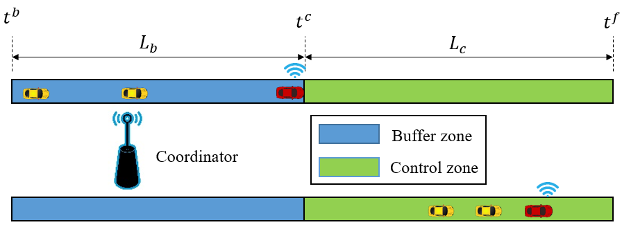
We consider a CAV followed by one or multiple HDVs traveling in a single-lane roadway of length . We subdivide the roadway into a buffer zone of length , inside of which the HDVs’ state information is estimated (Fig. 1) (top), and a control zone of length such that , where the CAV is controlled to form a platoon with the trailing HDVs, as shown in Fig. 1 (bottom). The time that a CAV enters the buffer zone, the control zone, and exits the control zone is , respectively.
Let , where is the total number of vehicles traveling within the buffer zone at time , be the set of vehicles considered to form a platoon. Here, the leading vehicle indexed by is the CAV, and the rest of the trailing vehicles in are HDVs. We denote the set of the HDVs following the CAV to be . Since the HDVs do not share their local state information with any external agents, we consider the presence of a coordinator that gathers the state information of the trailing HDVs traveling within the buffer zone. The coordinator, which can be a group of loop-detectors or comparable sensory devices, then transmits the HDV state information to the CAV at each time instance using standard vehicle-to-infrastructure communication protocol.
The objective of the CAV is to derive and implement a control input (acceleration/deceleration) at time so that the platoon formation with trailing HDVs in is completed within the control zone at a given time .
In our framework, we model the longitudinal dynamics of each vehicle as a double-integrator,
| (1) |
where , , and are the position of the front bumper, speed, and control input (acceleration/deceleration) of vehicle . Let denote the state vector of each vehicle , taking values in .
The speed and control input of each vehicle are subject to the following constraints,
| (2) |
where and are the minimum and maximum allowable speed of the considered roadway, respectively, and and are the minimum and maximum control input of all vehicles , respectively.
The dynamics (1) of each vehicle can take different forms based on the consideration of connectivity and automation. For the CAV , the control input can be derived and implemented within the control zone. We introduce and discuss the structure of the control zone in detail in Section III. To model the HDV dynamics, we need the following definitions.
Definition 1.
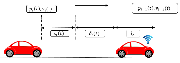
The dynamic following spacing between two consecutive vehicles is,
| (3) |
where denotes a desired time gap that each HDV maintains while following the preceding vehicle, and is the standstill distance denoting the minimum bumper-to-bumper gap at stop.
Definition 2.
The platoon gap is the difference between the bumper-to-bumper inter-vehicle spacing and the dynamic following spacing (see Fig. 2) between two consecutive vehicles , i.e.,
| (4) |
where is the length of each vehicle .
In this paper, we adopt the optimal velocity car-following model [14], to define the predecessor-follower coupled dynamics (see Fig. 2) of each HDV as follows,
| (5) |
where denotes the control gain representing the driver’s sensitivity coefficient, is the driver’s perception delay with a known upper bound , and denotes the equilibrium speed-spacing function,
Remark 1.
Based on (II), the driving behavior of each HDV depends on two different modes; (a) decoupled free-flow mode: when , each HDV converges to the maximum allowable speed , and cruises through the roadway decoupled from the state of the preceding vehicle, and (b) coupled following mode: when , the HDV dynamics becomes coupled with the state of the preceding vehicle , and converges to . Note that, if there is no preceding vehicle, we set that activates the decoupled free-flow mode, which results in converging to .
Remark 2.
We now provide the following definitions that are necessary for the formulation of our proposed platoon formation framework.
Definition 3.
The information set of the CAV has the following structure,
| (7) |
where .
Definition 4.
The steady-state traffic flow between two consecutive vehicles are established if the platoon gap does not vary with time, and speed fluctuation is zero [15], i.e.,
| (8) |
We now formalize the problem of platoon formation in mixed environment addressed in the paper as follows.
Problem 1.
Given the information set at time , the objective of the CAV is to derive the control input so that the HDVs in are forced to form a platoon at some time within the control zone while the following conditions hold,
| (9) |
where, denotes the equilibrium platoon speed.
Remark 3.
In our problem formulation, we impose the restriction that at , there exists at least one HDV such that . To simplify the formulation and without loss of generality, we consider that . This ensures that we do not have the trivial case where the group of vehicles in has already formed a platoon at .
In the modelling framework presented above, we impose the following assumption.
Assumption 1.
Remark 4.
We restrict the control of the CAV only within the control zone so that we have a finite control horizon . Outside the control zone, the CAV dynamics follows the car-following model in (5).
Lemma 1.
For each vehicle , .
Proof.
Since the control input of the uncontrolled CAV is determined by (5) outside the control zone (Remark 4), and due to the fact that any vehicle following the dynamics in (5) converges to the maximum speed without the presence of a preceding vehicle (Remark 1), converges to .
For a HDV traveling under the steady-state traffic flow condition (Assumption 1), does not vary with time. This implies that each HDV either travels with decoupled free-flow mode with , or with coupled following mode with . ∎
In what follows, first, we address Problem 1 considering only two vehicles, i.e., , and then generalize the analysis for multiple HDVs, i.e., .
III Vehicle Platoon Formation Framework
III-A Control input of CAV
The following result characterizes the control structure of CAV for the platoon formation framework.
Lemma 2.
For a CAV travelling with a trailing HDV , (i) a platoon formation does not occur when for all , and (ii) a platoon formation occurs with an appropriate control zone of length when for all .
Proof.
Part (i): For for all , we have for all , which implies that according to (9), no platoon formation will occur.
Part (ii): For within an arbitrary time horizon , we have . Since (Lemma 1), we have . This implies that decreases for all . As time progresses, given an appropriate control zone of length , we have , which guarantees a platoon formation. ∎
When the CAV applies a control input based on Lemma 2 to form a platoon with the HDV at time , two sequential steps take place, namely, (i) the platoon transition step, where the HDV transitions from the decoupled free-flow mode to the coupled following mode at time such that , and (ii) the platoon stabilization step, where converges to at time such that (9) is satisfied, and the platoon becomes stable.
Definition 5.
The platoon transition duration is the time required for the completion of the platoon transition step, i.e., , and the platoon stabilization duration is the time required for the completion of the platoon stabilization step, i.e., . Hence, we have .
Remark 5.
The platoon stabilization duration is , where is the perception delay of HDV , and is the response time of (5) which depends on the driver’s sensitivity coefficient , maximum allowable speed fluctuation, and the choice of equilibrium speed-spacing function in (II), and can be computed using stability analysis presented in [14, 16, 17]. Note that, for , additional nonlinearities may impact the computation of . In our formulation, we incorporate the upper bound of the perception delay to achieve robustness such that , and consider that is given a priori. Thus we focus only on the analysis of the platoon transition time .
Using Lemma 2, we construct the structure of the control input for the CAV for generating a platoon with the trailing HDV at time ,
According to (III-A), the realization of the control input of the CAV , which is in , yields a linearly decreasing in .
The following result provides the unconstrained relation between the platoon transition duration and CAV control input parameter .
Theorem 1.
For a CAV and a trailing HDV , there exists an unconstrained control input parameter in (III-A) such that a vehicle platoon can be formed with HDV at time according to the following condition,
| (12) |
Proof.
At , we require implying , which we expand as follows. Using (1) at time , we have . Based on Lemma 1, . For HDV , (Remark 3) until the platoon transition step at time . This implies, that HDV travels with decoupled free-flow mode as in (5), and for all (Lemma 1). Using (5) for HDV at time , we have, and . Substituting the last equation into (3), we have , and hence Simplifying using (4), the result follows. ∎
III-B Feasibility of the platoon formation time,
In Theorem 1, we do not explicitly incorporate the state and control constraints in (II), and the terminal constraint in (9). For a given platoon formation time , the corresponding control input derived from (12) can violate constraints in (II). In what follows, we present Lemmas 3 and 4 that provide a feasible region of that yields an admissible control input parameter in (12).
Lemma 3.
For CAV , the platoon transition duration subject to the state and control constraints in (II) is feasible if the following condition holds,
| (13) |
Proof.
Suppose that, for CAV , yields a corresponding platoon transition duration . From (12), we have . Therefore, for any to be feasible such that , we require , which yields the inequality with the first term in (13).
Now, suppose that for CAV , a platoon transition duration has associated control input parameter derived from (12). Using (1), we have, Since , we require that to satisfy the state constraint in (II). Substituting in the above inequality, we get . Finally, substituting from (12) in the above equation yields the inequality with the second term in (13).
Finally, since both above inequalities yield lower bounds on , we simply take their maximum and get (13). ∎
Remark 7.
Lemma 4.
For the CAV subject to the control input (III-A), the following condition must hold in order to complete platoon formation at time within the control zone of length ,
| (14) |
where, , and .
Proof.
The following result provides the condition under which for a given platoon formation time and platoon stabilization duration , the corresponding platoon transition duration is feasible.
Theorem 2.
For a CAV to complete the platoon transition step with its following HDV with control input within the control zone of length , a platoon transition duration is feasible if,
| (16) |
holds.
III-C Extension of the Analysis for
For , the CAV trailed by multiple HDVs and given , we have the following conditions, for all (Lemma 1), and there exists such that (Remark 3).
Definition 6.
For a CAV followed by HDVs, the cumulative platoon gap at time is,
| (17) |
In what follows, we extend the analysis presented in Theorems 1 and 2, and derive results that enables platoon formation considering multiple trailing HDVs, i.e., . The following theorem provides the unconstrained relation between the platoon transition duration and CAV control input parameter for .
Theorem 3.
For a CAV followed by HDVs , there exists an unconstrained control input parameter in (III-A) such that a vehicle platoon can be formed with HDVs at time according to the following relation,
| (18) |
Proof.
For , the following result provides the condition under which for a given platoon formation time and platoon stabilization duration , the corresponding platoon transition duration in Theorem 3 is feasible.
Theorem 4.
For a CAV to complete the platoon transition step with its following HDVs with control input within the control zone of length , a platoon transition duration is feasible if,
| (20) | |||
holds, where , , , and .
Proof.
Suppose that, for CAV , yields a corresponding platoon transition duration . From (18), we have , where .
Therefore, for any to be feasible such that , we require , which yields the inequality with the first term in (20).
Now for the second inequality term, since , we require that to satisfy the state constraint in (II). Using (1), we have, .
Substituting in the above inequality, we get . Substituting from (18) and simplifying, we have the inequality with the second term in (20). Since both left-hand side inequalities mentioned above give lower bounds on , we simply take their maximum and get the left inequality of (20).
Finally, using the result of Theorem 3 and following similar steps to those in the proofs of Lemma 4, we derive the right inequality of (20).
∎
IV Numerical Example
To demonstrate the performance of the proposed platoon formation framework, we present the simulation considering consisting of a CAV followed by two HDVs and , using numerical simulation in MATLAB R2020b. For a desired platoon formation time s and a given platoon stabilization duration s, s is feasible according to Theorem 4, and we use Theorem 3 to compute the corresponding control input for CAV . The headway trajectories of HDVs and converge to the equilibrium value and remain time invariant for all , as shown in Fig. 3 (bottom). Since the conditions in (9) are satisfied for all , the platoon formation is completed at time s as indicated by the position trajectories shown in Fig. 3 (top).

In Fig. 4, we show the robustness of the proposed framework in terms of platoon formation deviation representing the percentage deviation of the actual platoon formation time from the desired platoon formation time , i.e., , for . Here, positive platoon formation deviation indicates delayed platoon formation in actual simulation, and conversely, negative deviation indicates platoon formation before . Figure 4(a) shows that the platoon is formed within deviation for all admissible , where the higher values minimizes delayed platoon formation instances. The robustness of the framework under different perception delay is showed in Fig. 4(b). Since the platoon formation deviations are mostly non-positive, the conservative consideration of guarantees platoon formation within the desired platoon formation time .
Finally, we consider the variation of two car-following parameters, namely the desired time gap and driver’s sensitivity coefficient , to investigate the performance of the proposed framework under random human driving behavior based on (5), as shown in Fig. 4(c) and (d), respectively. The proposed framework is mostly robust against variation of , and shows delayed platoon formation only near the maximum value of . In contrast, the proposed framework shows delayed platoon formation with deviation for variation of . Note that, since is dependent on , the appropriate computation of can minimize the platoon formation deviation with varying .
Supplementary videos of the simulation and experimental results of the proposed framework as well as the parameters used for the simulation results can be found at: https://sites.google.com/udel.edu/platoonformation.
V Discussion and concluding Remarks
In this paper, we presented a framework for platoon formation under a mixed traffic environment, where a leading CAV derives and implements its control input to force the following HDVs to form a platoon. Using a predefined car-following model, we provided a complete, analytical solution of the CAV control input intended for the platoon formation. We also provided a detailed analysis of the platoon formation framework, and provided conditions under which a feasible platoon formation time exists. Finally, we presented numerical example to validate the robustness of our proposed framework.
A direction for future research should extend the proposed framework to make it agnostic to additional car-following models. Ongoing research considers the notion of optimality to derive energy- or time-optimal platoon formation framework under relaxed assumption on the steady-state traffic flow.

References
- [1] J. Guanetti, Y. Kim, and F. Borrelli, “Control of Connected and Automated Vehicles: State of the Art and Future Challenges,” Annual Reviews in Control, vol. 45, pp. 18–40, 2018.
- [2] J. Rios-Torres and A. A. Malikopoulos, “A Survey on Coordination of Connected and Automated Vehicles at Intersections and Merging at Highway On-Ramps,” IEEE Transactions on Intelligent Transportation Systems, vol. 18, no. 5, pp. 1066–1077, 2017.
- [3] A. M. I. Mahbub, L. Zhao, D. Assanis, and A. A. Malikopoulos, “Energy-Optimal Coordination of Connected and Automated Vehicles at Multiple Intersections,” in Proceedings of 2019 American Control Conference, 2019, pp. 2664–2669.
- [4] A. A. Malikopoulos, L. E. Beaver, and I. V. Chremos, “Optimal time trajectory and coordination for connected and automated vehicles,” Automatica, vol. 125, no. 109469, 2021.
- [5] A. I. Mahbub, A. A. Malikopoulos, and L. Zhao, “Decentralized optimal coordination of connected and automated vehicles for multiple traffic scenarios,” Automatica, vol. 117, no. 108958, 2020.
- [6] A. M. I. Mahbub and A. A. Malikopoulos, “Conditions to Provable System-Wide Optimal Coordination of Connected and Automated Vehicles,” Automatica, vol. 131, no. 109751, 2021.
- [7] A. M. I. Mahbub, A. Malikopoulos, and L. Zhao, “Impact of connected and automated vehicles in a corridor,” in Proceedings of 2020 American Control Conference, 2020. IEEE, 2020, pp. 1185–1190.
- [8] A. Alessandrini, A. Campagna, P. Delle Site, F. Filippi, and L. Persia, “Automated vehicles and the rethinking of mobility and cities,” Transportation Research Procedia, vol. 5, pp. 145–160, 2015.
- [9] Y. Zheng, S. E. Li, K. Li, and W. Ren, “Platooning of connected vehicles with undirected topologies: Robustness analysis and distributed h-infinity controller synthesis,” IEEE Transactions on Intelligent Transportation Systems, vol. 19, no. 5, pp. 1353–1364, 2017.
- [10] D. Hajdu, I. G. Jin, T. Insperger, and G. Orosz, “Robust design of connected cruise control among human-driven vehicles,” IEEE Transactions on Intelligent Transportation Systems, vol. 21, no. 2, pp. 749–761, 2019.
- [11] L. Zhao, A. A. Malikopoulos, and J. Rios-Torres, “Optimal control of connected and automated vehicles at roundabouts: An investigation in a mixed-traffic environment,” in 15th IFAC Symposium on Control in Transportation Systems, 2018, pp. 73–78.
- [12] A. R. Kreidieh, C. Wu, and A. M. Bayen, “Dissipating stop-and-go waves in closed and open networks via deep reinforcement learning,” in 2018 21st International Conference on Intelligent Transportation Systems (ITSC). IEEE, 2018, pp. 1475–1480.
- [13] C. Wu, K. Parvate, N. Kheterpal, L. Dickstein, A. Mehta, E. Vinitsky, and A. M. Bayen, “Framework for control and deep reinforcement learning in traffic,” in 2017 IEEE 20th International Conference on Intelligent Transportation Systems (ITSC). IEEE, 2017, pp. 1–8.
- [14] M. Bando, K. Hasebe, A. Nakayama, A. Shibata, and Y. Sugiyama, “Dynamical model of traffic congestion and numerical simulation,” Physical review E, vol. 51, no. 2, p. 1035, 1995.
- [15] R. W. Rothery, “Car following models,” Trac Flow Theory, 1992.
- [16] R. E. Wilson and J. A. Ward, “Car-following models: fifty years of linear stability analysis–a mathematical perspective,” Transportation Planning and Technology, vol. 34, no. 1, pp. 3–18, 2011.
- [17] L. Zhang, S. Zhang, B. Zhou, S. Jiao, and Y. Huang, “An improved car-following model considering desired safety distance and heterogeneity of driver’s sensitivity,” Journal of Advanced Transportation, vol. 2021, 2021.