On Angular Speed Estimation of Rigid Bodies
(Extended Version)

Handling rigid bodies, as in aerial or underwater vehicle applications, has been a source of control challenges for several decades now. In particular, the problem of estimating the state of a system evolving on the special group $\mathrm{SO}(3)$ has attracted the interest of researchers; see, e.g., [9, 11] and the references therein. It is worth noting that although the problem of attitude filtering has received a lot of attention, only a few contributions addressing angular speed estimation can be found. In [14] for instance, an observer based on quaternion description and discontinuous correction is proposed, and in [18], an observer is designed directly on $\mathrm{SO}(3)$, providing almost global asymptotic stability. In [1], another design on $\mathrm{SO}(3)$ can be found, providing global convergence. The strategy therein relies on a hybrid mechanism reminiscent of the results in [12]. Recently, angular speed estimators, yet for system spinning around a fixed axis have been presented in [2, 4].

The main contribution of this paper pertains to a novel observer for angular speed estimation of rigid bodies from attitude measurements on $\mathrm{SO}(3)$ expressed in an inertial frame. The key feature of the solution we propose consists of avoiding the common paradigm requiring to confine angular speed observers on the manifold $\mathrm{SO}(3)$. This enables to considerably simplify the structure and the convergence analysis of the observer, which does not require the use of sophisticated geometrical tools. The leading idea of our work is that estimating the angular speed does not require to estimate the attitude. This makes our approach unique when compared to recent results [1, 18]. The price to pay to obtain such a simplification is that our solution does not enable to obtain an estimate of the attitude [18].

The proposed methodology is specialized to the case of a body rotating around a fixed axis. This leads to an angular speed observer that can be exploited in the presence of “wrapped” angular measurements, which is a case of practical relevance. As an additional contribution, we show that in this setting, the observer can be coupled to a specific projection map and be also used for angular position filtering.

The remainder of the paper is organized as follows. Section II presents the problem we solve and the outline of the proposed observer. Section III provides sufficient conditions to ensure global asymptotic stability of the estimation error dynamics and characterizes robustness to small measurement noise. Section IV specializes the results presented in the previous sections to the specific, yet practically relevant, case of a body spinning around a fixed axis, and presents a thorough discussion about angular position estimation. Section V illustrates the proposed methodology in two numerical examples.

The symbol $\mathbb{R}_{\geq 0}$ ($\mathbb{R}_{>0}$) denotes the set of nonnegative (positive) reals, $\mathbb{R}^{n}$ is the Euclidean space of dimension $n$, $\mathbb{R}^{n\times m}$ is the vector space of $n\times m$ real matrices represented by the canonical basis, $\mathbb{S}_{+}^{n}$ is the set of $n\times n$ symmetric positive definite matrices, and $\mathbf{id}$ is the identity function. Given two topological spaces $X$ and $Y$, $\mathcal{C}^{0}(X;Y)$ is the set of continuous functions from $X$ to $Y$. For a matrix $M\in\mathbb{R}^{n\times m}$ (vector $x\in\mathbb{R}^{n}$), $M^{\mkern-1.5mu\mathsf{T}}$ ($x^{\mkern-1.5mu\mathsf{T}}$) denotes the transpose of $M$ (of $x$). For a symmetric matrix $M$, $M\succ 0$ denotes positive definiteness of $M$. Given a metric space $\mathcal{M}$, the symbol $\mathbb{B}$ denotes the closed unit ball in $\mathcal{M}$. For Euclidean vectors, we use the equivalent notation $(x,y)=[x^{\mkern-1.5mu\mathsf{T}}\,\,y^{\mkern-1.5mu\mathsf{T}}]^{\mkern-1.5mu\mathsf{T}}$. Let $\mathbb{U}$ be a normed linear vector space, $|x|$ stands for the norm of $x$. Let $x\in\mathbb{U}$ and $\mathcal{A}\subset\mathbb{U}$ be nonempty, the distance of $x$ to $\mathcal{A}$ is defined as $d(x,\mathcal{A})\coloneqq\displaystyle\inf_{y\in{\mathcal{A}}}|x-y|$. Let $A\in\mathbb{R}^{n\times n}$ and $B\in\mathbb{R}^{n\times n}$, $\langle A,B\rangle_{\mathcal{F}}\coloneqq\operatorname{trace}(A^{\mkern-1.5mu\mathsf{T}}B)$ denotes the Frobenius inner product, and $|A|_{\mathcal{F}}=\sqrt{\langle A,A\rangle_{\mathcal{F}}}$ the corresponding induced norm. The symbol $\mathfrak{so}(3)$ stands for the set of $3\times 3$ skew matrices and for any positive integer $n$, $\mathrm{SO}(n)\coloneqq\{R\in\mathbb{R}^{n\times n}\colon R^{\mkern-1.5mu\mathsf{T}}R=\mathbf{I},\det(R)=1\}$, where $\mathbf{I}$ denotes the identity matrix. Given $x\in\mathbb{R}^{3}$, we define $[x]_{\times}\coloneqq\left[\begin{smallmatrix}0&-x_{3}&x_{2}\\ x_{3}&0&-x_{1}\\ -x_{2}&x_{1}&0\end{smallmatrix}\right].$ Notice that $x\mapsto[x]_{\times}$ is invertible on $\mathfrak{so}(3)$. In particular, we denote the inverse of $x\mapsto[x]_{\times}$ by $\operatorname{vec}\colon\mathfrak{so}(3)\rightarrow\mathbb{R}^{3}$, defined as $\operatorname{vec}([x]_{\times})=x$. Let $\mathcal{U}$ be a finite dimensional real inner product space with dimension $n$, $V\colon\operatorname{dom}V\subset\mathcal{U}\rightarrow\mathbb{R}$, $x\in\mathcal{U}$, and $\{e_{i}\}_{i=1}^{n}$ be an orthonormal basis of $\mathcal{U}$, we use the notation $\nabla V(x)\coloneqq\sum_{i=1}^{n}(DV(x)e_{i})e_{i}$, where $DV(x)\colon\mathcal{U}\rightarrow\mathbb{R}$ stands for the differential of $V$ at $x$. For $f\colon X\rightarrow Y$, $\rge f$ stands for the image of $f$. The symbol $V^{-1}(c)$ stands for the $c$-level set of the function $V\colon\operatorname{dom}V\rightarrow\mathbb{R}$.

Next we state two useful properties. The first can be established by inspection.

In this paper we consider dynamical systems of the form:

where $x\in\mathcal{U}$ is the system state, $\mathcal{U}$ is a normed finite dimensional linear vector space, $C\subset\mathcal{U}$, and the set valued map $F\colon\operatorname{dom}F\rightrightarrows\mathcal{U}$. In particular, we say that (1) satisfies the so-called basic conditions if: $C$ is closed in $\mathcal{U}$, $F$ is outer semicontinuous and locally bounded on $C$, $C\subset\operatorname{dom}F$, and for all $x\in C$, $F(x)$ is convex. A function $\phi\colon\operatorname{dom}\phi\rightarrow\mathcal{U}$ is a solution to (1) if $\operatorname{dom}\phi$ is an interval of $\mathbb{R}_{\geq 0}$ including zero, $\phi(0)\in C$, $\phi$ is locally absolutely continuous, and for almost all $t\in\operatorname{dom}\phi$, $\phi(t)\in C$ and $\dot{\phi}(t)\in F(\phi(t))$. A solution to (1) is said to be maximal if its domain cannot be extended and complete if its domain is unbounded. The following stability notion for compact sets is considered.

The following definition is used in the paper.

See [8] for more details on these assumptions and definitions for the more general case of hybrid dynamical systems.

Before stating the main result of this section, we recall the following obvious result that applies to (2).

In the result given next, we provide sufficient conditions on the nonlinear gain $\Gamma$ and on the gain $K$ to ensure global pre-asymptotic stability of the set $\mathcal{A}$ for (5). The result relies on the use of an invariance principle, whose application is enabled by the fact that (5) satisfies the basic conditions (see Lemma 1); see [15] for more details on invariance principles for constrained differential inclusions.

We assume that measurements of the rotation matrix $\mathcal{R}$ are affected by a bounded additive measurement noise $\eta\in\mathbb{R}^{3\times 3}$. In this scenario, the interconnection of the plant and the observer can be modeled as

where for all $x\in\mathcal{X},\eta\in\mathbb{R}^{3\times 3}$, $F_{n}(x,\eta)$ are the dynamics of $x$ when $\mathcal{R}$ is replaced by $\mathcal{R}+\eta$ in the observer dynamics (3) and $\mathcal{O}\subset\mathcal{U}$ is an arbitrary compact set that is introduced to simplify the analysis.

Following Section II, we propose the following observer⁸⁸ 8 A reduced order observer may be easily derived by replacing the measurement $R$ by $Rv$, with $0\neq v\in\mathbb{R}^{2}$. However, the resulting observer cannot be employed for angular position filtering as in Section IV-B.:

where $\Gamma\in\mathcal{C}^{0}(\mathbb{R}^{2\times 2};\mathbb{R}^{2\times 2})$ and $\kappa\in\mathbb{R}$ are to be designed. By introducing the error coordinates $\widetilde{R}\coloneqq R-\widehat{R}$, $\tilde{\omega}\colon=\omega-\hat{\omega}$, the interconnection of (17) and (18) can be written as the following dynamical system with state $\chi\coloneqq(R,\omega,\widetilde{R},\tilde{\omega})\in\mathcal{V}\coloneqq\mathbb{R}^{2\times 2}\times U\times\mathbb{R}^{2\times 2}\times\mathbb{R}$

where $\mathcal{T}\coloneqq\mathrm{SO}(2)\times U\times\mathbb{R}^{2\times 2}\times\mathbb{R}$.

Similarly to Section III, we introduce the compact set:

wherein the estimation error is equal to zero and provide sufficient conditions for global pre-asymptotic stability of $\mathcal{W}$.

The above result can be easily proven via a simple adaptation of the proof of Theorem 1, therefore its proof is omitted.

The objective of the proposed observer is to generate an estimate of the angular speed based on attitude measurements. In this section, we briefly discuss about the problem of attitude filtering, which is a relevant problem in the presence of noisy measurements. As mentioned in Section II, the proposed observer does not provide a meaningful estimate of the attitude. A possible approach to solve this problem consists of computing online the “nearest” rotation matrix to the estimate generated by the observer. However, obtaining a closed-form expression of such a “projection” operation turns out to be a difficult problem; see [16]. Nonetheless, in this section we show how such an explicit expression can be obtained in the context of $\mathrm{SO}(2)$.

The set of nearest matrices to a given matrix $H\in\mathbb{R}^{2\times 2}$ can be implicitly represented by the set-valued map $\Pi\colon\mathbb{R}^{2\times 2}\rightrightarrows\mathrm{SO}(2)$ defined for all $H\in\mathbb{R}^{2\times 2}$ as:

The result given next provides a closed-form expression of the set valued map $\Pi$.

The property below holds for set valued map $\Pi$.

Lemma 2 ensures that for all $\mathbb{R}_{\geq 0}\ni t\mapsto R(t)\in\mathrm{SO}(2)$ and $\mathbb{R}_{\geq 0}\ni t\mapsto\widetilde{R}(t)$, the following implication holds:

Roughly speaking, this ensures that projecting $\widehat{R}$ onto $\mathrm{SO}(2)$ yields a proper converging estimate of the attitude $R$.

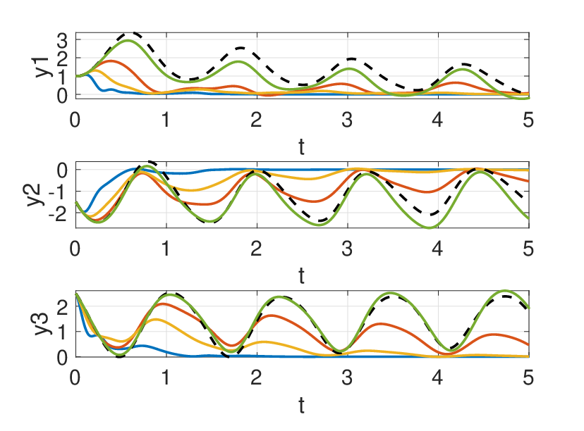
In this example, we showcase the effectiveness of the results proposed in Section III via numerical simulations. In particular, we consider the scenario of [18, Section V] in which $J_{0}=\begin{bmatrix}5&0&0\\ 0&1&0\\ 0&0&2\end{bmatrix}$ and (2) is initialized as $\mathcal{R}(0)=\exp(\pi/4[e_{1}]_{\times})$, $\omega(0)=(1,-1.5,2.5)$, where $e_{1}=(1,0,0)$. The observer (3) is initialized at $\widehat{\mathcal{R}}(0)=\mathcal{R}_{0},\hat{q}(0)=0$ and for simplicity we set $u=0$. Fig. 1 depicts the evolution of $\omega-\hat{\omega}$ with $\Gamma=20\mathbf{id}$ and different selections of $K$ and $\Gamma$. Fig. 1 clearly shows that the proposed observer yields a converging estimate of $\omega$ and underlines the impact of the parameters $K$ and $\Gamma$ on the convergence speed. Namely, for $K=100J_{0}$ and $\Gamma=20\mathbf{id}$ the proposed observer practically converges in $1.5$ seconds, which appears to be much faster when compared with the numerical results in [18]. Notice also that for the same selection of $K$, taking $\Gamma=10^{3}\mathbf{id}$ negatively affects the convergence speed.

To assess the impact of measurement noise on the observer, in Fig. 2 we report the evolution of $\omega-\hat{\omega}$ (after transient) in the presence of a band-limited white measurement noise. The figure underlines that fast convergence speed comes at the price of increased noise sensitivity.

In this section, we illustrate the results of Section IV via numerical simulations. As in [2, 4], we assume to have access to measurements of the angular position $\theta$ wrapped in the interval $(-\pi,\pi]$ and map those to $\mathrm{SO}(2)$ via the standard bijection from $(-\pi,\pi]$ to $\mathrm{SO}(2)$. Fig. 3 shows the evolution of $\theta,\omega$, $\hat{\omega}$, and $\hat{\theta}$ from the following initial condition: $\theta(0)=\pi/2$, $\widehat{R}(0)=\mathbf{I}$, $\omega(0)=10$, $\hat{\omega}(0)=0$, when $\Gamma=40\mathbf{id}$ and $K=200$. The estimate $\hat{\theta}$ is obtained via (22) by mapping $\Pi(\widehat{R})\in\mathrm{SO}(2)$ to $(-\pi,\pi]$. The picture points out that, despite wrapped measurements, the proposed observer provides a convergent estimate of the angular speed. To illustrate the results of Section IV-B, we perform some simulations in which angular measurements are affected by a bounded additive noise $\eta(t)=0.1\sin(10^{4}t)$. Fig. 4 reports the evolution of the estimate $\hat{\theta}$ of the angular position along with the angular speed estimation error. Simulations show that the proposed observer is robust to measurement noise and that the attitude filtering technique of Section IV-B is effective in yielding a smoother estimate of the angular position.

References

• [1] S. Berkane, A. Abdessameud, and A. Tayebi. Global exponential angular velocity observer for rigid body systems. In Proceedings of the 55th IEEE Conference on Decision and Control, pages 4154–4159, 2016.
• [2] P. Bernard and L. Praly. Estimation of position and resistance of a sensorless pmsm: a nonlinear Luenberger approach for a non-observable system. IEEE Transactions on Automatic Control, 2020.
• [3] D. S. Bernstein. Matrix mathematics: theory, facts, and formulas. Princeton university press, 2009.
• [4] M. Brentari, P. Bosetti, and L. Zaccarian. A class of hybrid velocity observers for angular measurements with jumps. IEEE Control systems letters, 2(4):617–622, 2018.
• [5] C. Cai and A. R. Teel. Characterizations of input-to-state stability for hybrid systems. Systems & Control Letters, 58(1):47–53, 2009.
• [6] F. Ferrante and Y. Wang. A hybrid systems approach to splay state stabilization of pulse coupled oscillators. In Proceedings of the IEEE 55th Conference on Decision and Control, pages 1763–1768, 2016.
• [7] F. Ferrante and Y. Wang. Robust almost global splay state stabilization of pulse coupled oscillators. IEEE Transactions on Automatic Control, 62(6):3083–3090, 2017.
• [8] R. Goebel, R. G. Sanfelice, and A. R. Teel. Hybrid Dynamical Systems: Modeling, Stability and Robustness. Princeton UNiversity Press, 2012.
• [9] M. F. Haydar and M. Lovera. ℋ∞\mathcal{H}_{\infty} filtering on the unit circle. In Proceedings of the IEEE 56th Conference on Decision and Control, pages 2422–2427, 2017.
• [10] Y. Li and R. G. Sanfelice. A finite-time convergent observer with robustness to piecewise-constant measurement noise. Automatica, 57:222–230, 2015.
• [11] R. Mahony, T. Hamel, and J.-M. Pflimlin. Nonlinear complementary filters on the special orthogonal group. IEEE Transactions on Automatic Control, 53(5):1203–1218, 2008.
• [12] C. G. Mayhew and A. R. Teel. Synergistic hybrid feedback for global rigid-body attitude tracking on 𝐒𝐎⁡(3)\mathbf{SO}(3). IEEE Transactions on Automatic Control, 58(11):2730–2742, 2013.
• [13] F. Nunez, Y. Wang, A. R. Teel, and F. J. Doyle III. Synchronization of pulse-coupled oscillators to a global pacemaker. Systems & Control Letters, 88:75–80, 2016.
• [14] S. Salcudean. A globally convergent angular velocity observer for rigid body motion. IEEE Transactions on Automatic Control, 36(12):1493–1497, 1991.
• [15] Ricardo G Sanfelice, Rafal Goebel, and Andrew R Teel. Invariance principles for hybrid systems with connections to detectability and asymptotic stability. IEEE Transactions on Automatic Control, 52(12):2282–2297, 2007.
• [16] S. Sarabandi, A. Shabani, J. M. Porta, and F. Thomas. On closed-form formulas for the 3−d3-d nearest rotation matrix problem. IEEE Transactions on Robotics, 36(4):1333–1339, 2020.
• [17] I. Sarras. Global exponential estimation of rigid body angular velocity directly from multiple vector measurements. In Proceedings of European Control Conference, pages 979–984, 2020.
• [18] T.-H. Wu and T. Lee. Angular velocity observer for velocity-free attitude tracking control on S​O​(3)SO(3). In Proceedings of the European Control Conference, pages 1824–1829, 2015.
-A Additional details for the proof of Theorem 1
The proof of Theorem 1 relies on the computation of vector ∇V​(ℛ~,q~)\nabla V(\widetilde{\mathcal{R}},\tilde{q}), where
(ℛ~,q~)↦V⁡(ℛ~,q~)=12​⟨ℛ~,ℛ~⟩ℱ+12​q~𝖳​K−1​q~(\widetilde{\mathcal{R}},\tilde{q})\mapsto V(\widetilde{\mathcal{R}},\tilde{q})=\frac{1}{2}\langle\widetilde{\mathcal{R}},\widetilde{\mathcal{R}}\rangle_{\mathcal{F}}+\frac{1}{2}\tilde{q}^{\mkern-1.5mu\mathsf{T}}K^{-1}\tilde{q}
which enables to express the directional derivative of x↦V⁡(ℛ~,q~)x\mapsto V(\widetilde{\mathcal{R}},\tilde{q}) along the dynamics of system (5) as
⟨∇V​(ℛ~,q~),h​(x)⟩\langle\nabla V(\widetilde{\mathcal{R}},\tilde{q}),h(x)\rangle
where for all x∈𝒳x\in\mathcal{X}
h⁡(x)≔[[ℛ​J0−1​ℛ𝖳​q~]×​ℛ−Γ⁡(ℛ~)−K​ℛ​J0−1​ℛ𝖳​vec⁡(ℛ~​ℛ𝖳−ℛ​ℛ~𝖳)],h(x)\coloneqq\begin{bmatrix}[\mathcal{R}J_{0}^{-1}\mathcal{R}^{\mkern-1.5mu\mathsf{T}}\tilde{q}]_{\times}\mathcal{R}-\Gamma(\widetilde{\mathcal{R}})\\ -K\mathcal{R}J_{0}^{-1}\mathcal{R}^{\mkern-1.5mu\mathsf{T}}\operatorname{vec}(\widetilde{\mathcal{R}}\mathcal{R}^{\mkern-1.5mu\mathsf{T}}-\mathcal{R}\widetilde{\mathcal{R}}^{\mkern-1.5mu\mathsf{T}})\end{bmatrix},
and for all (R1,q1),(R2,q2)∈ℝ3×3×ℝ3(R_{1},q_{1}),(R_{2},q_{2})\in\mathbb{R}^{3\times 3}\times\mathbb{R}^{3}, ⟨(R1,q1),(R2,q2)⟩≔⟨R1,R2⟩ℱ+q1𝖳​q2.\langle(R_{1},q_{1}),(R_{2},q_{2})\rangle\coloneqq\langle R_{1},R_{2}\rangle_{\mathcal{F}}+q_{1}^{\mkern-1.5mu\mathsf{T}}q_{2}.
By definition
∇V​(ℛ~,q~)=∑i=112(D​V​(ℛ~,q~)​ei)​ei∈ℝ3×3×ℝ3\nabla V(\widetilde{\mathcal{R}},\tilde{q})=\sum_{i=1}^{12}(DV(\widetilde{\mathcal{R}},\tilde{q})e_{i})e_{i}\in\mathbb{R}^{3\times 3}\times\mathbb{R}^{3}
where {ei}i=112\{e_{i}\}_{i=1}^{12} is any orthonormal basis of ℝ3×3×ℝ3\mathbb{R}^{3\times 3}\times\ \mathbb{R}^{3} (endowed with the standard inner product ⟨⋅,⋅⟩ℱ+⟨⋅,⋅⟩ℝ3\langle\cdot,\cdot\rangle_{\mathcal{F}}+\langle\cdot,\cdot\rangle_{\mathbb{R}^{3}}). In particular, ∇V​(ℛ~,q~)\nabla V(\widetilde{\mathcal{R}},\tilde{q}) is the Riesz representation of D​V​(ℛ~,q~)DV(\widetilde{\mathcal{R}},\tilde{q}), which, being unique, does not depend on the basis {ei}i=112\{e_{i}\}_{i=1}^{12}. To perform this computation, we select the canonical basis of ℝ3×3×ℝ3\mathbb{R}^{3\times 3}\times\ \mathbb{R}^{3}, that is:
({Ei}i=19×{0})∪({0}×{gi}i=13)\left(\{E_{i}\}_{i=1}^{9}\times\{0\}\right)\cup\left(\{0\}\times\{g_{i}\}_{i=1}^{3}\right)
where {Ei}\{E_{i}\} and {gi}\{g_{i}\} are, respectively, the canonical basis of ℝ3×3\mathbb{R}^{3\times 3} and ℝ3\mathbb{R}^{3}. Following this approach, it easy to see that for all (e,0)∈({Ei}i=19×{0})(e,0)\in\left(\{E_{i}\}_{i=1}^{9}\times\{0\}\right), one has
(D​V​(ℛ~,q~)​(e,0))​(e,0)=⟨ℛ~,e⟩ℱ(DV(\widetilde{\mathcal{R}},\tilde{q})(e,0))(e,0)=\langle\widetilde{\mathcal{R}},e\rangle_{\mathcal{F}}
and that for all (0,w)∈({0}×{gi}i=13)(0,w)\in\left(\{0\}\times\{g_{i}\}_{i=1}^{3}\right)
(D​V​(ℛ~,q~)​(0,w))​(0,w)=q~𝖳​K−1​w(DV(\widetilde{\mathcal{R}},\tilde{q})(0,w))(0,w)=\tilde{q}^{\mkern-1.5mu\mathsf{T}}K^{-1}w
Thus
∇V​(ℛ~,q~)=(ℛ~,K−1​q~)∈ℝ3×3×ℝ3\nabla V(\widetilde{\mathcal{R}},\tilde{q})=(\widetilde{\mathcal{R}},K^{-1}\tilde{q})\in\mathbb{R}^{3\times 3}\times\mathbb{R}^{3}
-B Discussion on wrapped angular measurements.
The set SO⁡(2)\mathrm{SO}(2) is isomorphic to the set of equivalence classes [−π,π]/∼[-\pi,\pi]/\sim, where ∼\sim is the “gluing” equivalence: x∼x′x\sim x^{\prime} if x=x′x=x^{\prime} or x=−πx=-\pi and x′=πx^{\prime}=\pi, or x=πx=\pi and x′=−πx^{\prime}=-\pi. The isomorphism is given by
([−π,π]/∼)∋[x]↦f(x)=[cos⁡(x)−sin⁡(x)sin⁡(x)cos⁡(x)]∈SO(2)\displaystyle([-\pi,\pi]/\sim)\ni[x]\mapsto f(x)=\begin{bmatrix}\cos(x)&-\sin(x)\\ \sin(x)&\cos(x)\end{bmatrix}\in\mathrm{SO}(2)
SO⁡(2)∋y↦f−1​(y)={{atan2⁡(y21,y11)}if​y21≠0{±π}else\displaystyle\mathrm{SO}(2)\ni y\mapsto f^{-1}(y)=\begin{cases}\{\mathrm{atan2}(y_{21},y_{11})\}&\text{if}\,\,y_{21}\neq 0\\ \{\pm\pi\}&\text{else}\end{cases}
where [x][x] stands for the equivalence class of x∈[−π,π]x\in[-\pi,\pi] and atan2\mathrm{atan2} stands for the 2-argument arctangent function. Clearly ff is continuous, while continuity of f−1f^{-1} can be proven by observing that f−1f^{-1} sends closed sets in SO⁡(2)\mathrm{SO}(2) into closed sets into [−π,π]/∼[-\pi,\pi]/\sim. In this sense, wrapped measurements of the angular position can be thought as the image in (−π,π](-\pi,\pi] of points in ([−π,π]/∼)([-\pi,\pi]/\sim) through the map:
g⁡([x])={xif​[x]∩{±π}=∅πelseg([x])=\begin{cases}x&\text{if}\,\,[x]\cap\{\pm\pi\}=\emptyset\\ \pi&\text{else}\end{cases}
It can be shown that gg is discontinuous and this is what leads to “jumps” in wrapped measurements.