The Hubble Tension as a Hint of Leptogenesis and Neutrino Mass GenerationPreprint: TUM-HEP 1318/21
Abstract
The majoron, a neutrinophilic pseudo-Goldstone boson conventionally arising in the context of neutrino mass models, can damp neutrino free-streaming and inject additional energy density into neutrinos prior to recombination. The combination of these effects for an eV-scale mass majoron has been shown to ameliorate the outstanding tension, however only if one introduces additional dark radiation at the level of . We show here that models of low-scale leptogenesis can naturally source this dark radiation by generating a primordial population of majorons from the decays of GeV-scale sterile neutrinos in the early Universe. Using a posterior predictive distribution conditioned on Planck2018+BAO data, we show that the value of observed by the SH0ES collaboration is expected to occur at the level of in the primordial majoron cosmology (to be compared with in the case of CDM). This insight provides an intriguing connection between the neutrino mass mechanism, the baryon asymmetry of the Universe, and the discrepant measurements of .
I Introduction
The Hubble Tension, circa early 2021. Despite its simplicity, the standard cosmological model (i.e. CDM) has proven to be remarkably successful in describing the vast array of cosmological observations at hand. However in recent years, a growing discrepancy has emerged between the value of as predicted by CDM Aghanim et al. 2020a; Aghanim et al. 2020b; Abbott et al. 2018; Addison et al. 2018; Schöneberg et al. 2019; Cuceu et al. 2019, and local observations that favor a significantly larger value, with a central values ranging between , coming from e.g. type Ia supernovae Riess et al. 2016; Riess et al. 2019; Dhawan et al. 2018; Burns et al. 2018; Riess et al. 2018; Freedman et al. 2019; Yuan et al. 2019; Reid et al. 2019; Riess et al. 2021, strong gravitational lensing Bonvin et al. 2017; Birrer et al. 2019; Rusu et al. 2020; Chen et al. 2019; Wong et al. 2020, surface brightness fluctuations Blakeslee et al. 2021, and megamasers Reid et al. 2009 (see e.g. Verde et al. 2019; Riess 2019 for recent reviews). This tension has now reached a significance quantified at the level Riess 2019, and appears across an array of different datasets with seemingly independent systematics. It is thus necessary to now consider the very real possibility that this discrepancy is arising from a failure of the CDM model to accurately describe the evolution of the Universe.
In this light, a large number of potential solutions have been proposed which typically fall into one of two categories: those which modify the Universe at late times () and those which modify the dynamics and evolution near recombination () – we refer the reader to Martsell and Dhawan 2018; Poulin et al. 2018; Nunes 2018; Di Valentino et al. 2020; Vattis et al. 2019; Li et al. 2019; Visinelli et al. 2019; Yang et al. 2021 and to Poulin et al. 2019; Agrawal et al. 2019; Lin et al. 2019; Smith et al. 2020; D’Eramo et al. 2018; Escudero et al. 2019; Bringmann et al. 2018; Pandey et al. 2020; Blinov et al. 2020; Blinov and Marques-Tavares 2020; Lancaster et al. 2017; Kreisch et al. 2020; Park et al. 2019; Sakstein and Trodden 2020; Archidiacono et al. 2020; Choi et al. 2020; Freese and Winkler 2021 for several recent proposals of each type, and to Di Valentino et al. 2021 for a recent comprehensive review of models. Cosmological observations from type Ia supernovae and baryonic acoustic oscillations (BAO) severely limit the viability of late-time solutions (see e.g. Bernal et al. 2016; Aylor et al. 2019; Knox and Millea 2020). In order for early Universe solutions to be successful in raising the inferred value of , one must modify the expansion rate near recombination. While these models often struggle to maintain the high-quality fit to CMB data that is obtained in CDM, this classification of solutions has proven thus far to be most successful in producing agreement between all cosmological datasets – see Knox and Millea 2020. Finding meaningful ways to motivate the novel physics required, however, has been challenging – many of the proposed solutions require complicated and un-motivated models which are fine-tuned in order to ensure that the effects ‘turn-on’ at the correct epoch and produce sufficiently sizable shift in .

The Hubble tension and a light Majoron. Recently, in Ref. Escudero and Witte 2020 (see also Escudero Abenza and Witte 2020 for a short summary), the authors illustrated that a light majoron, naturally arising in neutrino mass models from the spontaneous breaking of a global lepton number symmetry Chikashige et al. 1981; Gelmini and Roncadelli 1981; Georgi et al. 1981; Schechter and Valle 1982, could partially counteract the effect of additional dark radiation (i.e. ), pushing the inferred value of to larger values while maintaining a good fit to the CMB data. The presence of the majoron has two effects Chacko et al. 2004. First, the interactions damp the free streaming nature of neutrinos, which in turn damps the anisotropic stress; since the anisotropic stress sources the metric, the net effect is a time-dependent modification to the growth of potential wells Bashinsky and Seljak 2004. Second, for large enough interactions, the majorons can thermalize with neutrinos between Big Bang Nucleosynthesis (BBN) and recombination. Upon becoming non-relativistic these majorons decay back into neutrinos, producing a net enhancement in Chacko et al. 2004; Escudero and Witte 2020. Ensuring the effects of the majoron occur at the correct epoch requires a mass near the eV scale; this scale, however, is not arbitrary, and can easily be motivated should global lepton number be explicitly broken by physics at the Planck scale Rothstein et al. 1993; Akhmedov et al. 1993, as might be expected in theories of quantum gravity Kallosh et al. 1995; Banks and Seiberg 2011; Witten 2018; Harlow and Ooguri 2019; Fichet and Saraswat 2020; Alvey and Escudero 2021. In order to generate a sufficient level of damping one requires neutrino-majoron couplings Escudero and Witte 2020; Escudero Abenza and Witte 202011 1 The model discussed here has, on occasion, been confused with that of the strongly interaction neutrino solution proposed in Kreisch et al. 2020; Park et al. 2019. In light of this, we take the opportunity here to highlight the many differences. First, the solution of Kreisch et al. 2020; Park et al. 2019 requires a neutrino self-interaction cross section 10 orders of magnitude larger than that present in the Standard Model. This, in turn, requires a new -scale neutrinophilic boson with order one couplings. These values are not motivated in neutrino mass models, and are robustly excluded by experimental data unless the boson interacts only with neutrinos Blinov et al. 2019; Lyu et al. 2021; Brdar et al. 2020. Next, the solution requires an additional contribution of , a value robustly excluded by BBN Pitrou et al. 2018; Fields et al. 2020 – see also Huang and Rodejohann 2021; Seto and Toda 2021 for a recent assessment of the BBN bounds and Berbig et al. 2020; He et al. 2020 for models trying to evade these constraints. Finally, the observed shift in only occurs when polarization data is not included in the fit Kreisch et al. 2020; Roy Choudhury et al. 2020; Das and Ghosh 2020; Brinckmann et al. 2020, while the results for the majoron model discussed here are robust to the inclusion of this dataset. Thus, while the proposed models both involve neutrinophilic bosons, they are in fact remarkably different.. This coupling, when interpreted in the context of the type-I seesaw favors a lepton symmetry breaking scale slightly above the electroweak scale (). Arguably, the only unmotivated aspect of this proposed solution is the apparent ad hoc contribution of , preferring values , which are in mild tension with BBN Pitrou et al. 2018; Fields et al. 2020.
Primordial Majorons from Leptogenesis. In this work we attempt to source the additional dark radiation required to resolve the tension from a primordial population of majorons. We show explicitly that these particles can be produced from the decays of GeV-scale sterile neutrinos in the early Universe. Coincidentally, sterile neutrinos at the GeV scale are precisely those required for a successful implementation of low-scale leptogenesis via sterile neutrino oscillations, i.e. ARS leptogenesis Akhmedov et al. 1998 (see also Asaka and Shaposhnikov 2005; Shaposhnikov 2008; Drewes et al. 2018). We verify explicitly that symmetry breaking scales required to resolve the Hubble tension can be made fully consistent with conventional ARS leptogenesis, so long as the Higgs mixing is small enough so as to avoid thermalizing the scalar responsible for breaking lepton number, and that the lepton number phase transition occurs at . The scenario proposed here thus offers an intriguing connection between the tension, the neutrino mass mechanism, and the generation of the baryon asymmetry of the Universe. Fig. 1 shows a sketch of the thermal history, highlighting the main ingredients of our proposal.
This manuscript is organized as follows. We begin by introducing the well-known singlet majoron model in Section II. In Section III we first discuss the requirements in order to successfully produce the baryon asymmetry of the Universe via the ARS leptogenesis mechanism, and then compute the thermal evolution and subsequent decays of the sterile neutrinos responsible for sourcing the primordial majoron abundance. Section IV describes the cosmological evolution of the majoron-neutrino system, and presents the results of a MCMC performed using Planck2018 + BAO data. We present a summary and our conclusions in Section V. We finish in Section VI by discussing some interesting avenues for future work, and we refer the reader to the Appendices for various technical details.
II The Singlet Majoron Model
Throughout this manuscript we work with the well-known singlet majoron model Chikashige et al. 1981 (see also Schechter and Valle 1982) in which Majorana masses for the right-handed neutrinos are generated from the spontaneous breaking of a global lepton number symmetry22 2 Global symmetries are also expected to be explicitly broken by quantum gravity Kallosh et al. 1995; Banks and Seiberg 2011; Witten 2018; Harlow and Ooguri 2019; Fichet and Saraswat 2020; Alvey and Escudero 2021. This has two important consequences. First, this breaking will generate a mass for the majoron; if the breaking is perturbative, one can show that dimension 5 Planck-suppressed operators naturally generate masses in the range keV Rothstein et al. 1993; Akhmedov et al. 1993, which coincidentally overlaps with the range of interest for the Hubble tension (see Escudero and Witte 2020 for a discussion). Additionally, an explicit breaking of the symmetry guarantees that topological defects will naturally decay on short timescales Vilenkin and Everett 1982; Kawasaki and Nakayama 2013, and thus consequently pose no threat of over-closing the Universe.. In this set-up, the small neutrino masses then arise from the type-I seesaw mechanism Minkowski 1977; Mohapatra and Senjanovic 1981; Gell-Mann et al. 1979; Yanagida 1980; Schechter and Valle 1980.
This model is realized by augmenting the Standard Model (SM) with right handed neutrinos with lepton number and a scalar field with , all singlets under the SM gauge group. This particle content and charge arrangements, together with the requirement of renormalizability of the interactions, leads to the following Lagrangian
| (1) |
where are the - Yukawa couplings, and are the Higgs-Lepton- Yukawa couplings. The scalar potential is given by
| (2) |
Upon spontaneous symmetry breaking (SSB) of the symmetry, the scalar acquires a vacuum expectation value and will generate Majorana masses for the sterile neutrinos . Since is a global symmetry, a pseudo-Goldstone boson appears on the spectrum: the majoron Chikashige et al. 1981. After SSB, it is convenient to parametrize as
| (3) |
where is a CP even scalar, which in the limit will have a tree level mass given by .
Only after the SSB of the electroweak symmetry will Dirac neutrino masses appear, with . Diagonalizing the neutrino mass matrix in the limit yields light active Majorana neutrinos with masses of the order:
| (4) |
Assuming no strong cancellations occur, one typically expects the heavy sterile neutrinos to have very small mixings with light active states (see Casas and Ibarra 2001 for a general case), with a magnitude roughly given by
| (5) |
and with Higgs’ Yukawa couplings of the order
| (6) |
One of the conventional appeals of the seesaw mechanism is that the fine-tuning of the Yukawa couplings required to generate the active neutrino masses can be ameliorated when . Successful low-scale leptogenesis, however, requires GeV-scale sterile neutrino masses, which are capable of reducing, but not removing the aforementioned fine-tuning problem (see Eq. (6)). While this naively appears to remove at least part of the original appeal, it is worth emphasizing that there exist mixing textures (i.e. non-trivial )33 3 In this context, we refer to Arias-Aragon et al. 2021 for a recent embedding of our set up within the minimal lepton flavor violating framework. which can substantially enhance relative to the value quoted in Eq. (5) (and further remove any need for tuning), however for the sake of simplicity and concreteness we choose to work within the prototypical seesaw limit.
A. Neutrino-Majoron Interactions
With Eq. (II) in hand, one can enumerate the novel interactions that arise between the neutrinos (both active and sterile), the majoron, and . Working in the mass basis of and , the relevant interactions in the seesaw limit are Pilaftsis 1992; Pilaftsis 1994
| (7) |
where the couplings are given by44 4 Notice that Eq. (10) is smaller by a factor of 2 with respect to the one used in Escudero and Witte 2020. We are grateful to Manuel Masip for pointing out this error.
| (8) | ||||
| (9) | ||||
| (10) |
Here we have omitted generation indices, however this is valid when considering the three light neutrino mass eigenstates as is a diagonal matrix up to tiny corrections Schechter and Valle 1982. It is worth highlighting that interactions between the majoron and charged fermions are both neutrino mass and loop-suppressed, and are thus expected to appear at the level of Chikashige et al. 1981. The majoron is thus, for all intents, a truly neutrinophilic boson.
There are two interactions in particular that are worth mentioning at this point. In order to generate a sizable primordial population of majorons in the very early Universe (), we must require sterile neutrinos to efficiently decay into majorons, and in order to ensure majorons thermalize with neutrinos at late-times, we must ensure the inverse decay of active neutrinos to majorons exceeds the Hubble rate near recombination. As we shall see, both of these requirements are satisfied for values of and .
Let us begin by assuming sterile neutrinos have thermalized at temperatures , and identify the condition necessary to generate a sizable branching fraction to majorons. The decay rate of sterile neutrinos into a majoron and active neutrino is
| (11) |
This should be compared with the decay rate into SM particles, which for sterile neutrino masses is roughly given by (see e.g. Gonzalez-Garcia et al. 1990), where
| (12) |
Therefore, the ratio between the decay rates is
| (13) |
implying a branching ratio for all relevant parameter space.
We will show explicitly in the next section that in order for the majoron solution to remain viable (at least in the seesaw limit), we require to be TeV and GeV; the former is necessary in order to ensure neutrino-majoron interactions can damp the neutrino anisotropic stress, and the latter is required in order to generate a sufficiently large contribution to (if sterile neutrinos decay at earlier times the energy density of any majoron population produced will be diluted by subsequent entropy dumps). Eq. (13) then shows that sterile neutrino decays will be efficient in generating majorons across the entirety of the parameter space of interest.
Now let us turn our attention to the late-time phenomenology, where we must require majorons to thermalize with active neutrinos near recombination. For the small couplings and masses of interest (), this process proceeds via the inverse decays of active neutrinos (). The efficiency of this process is governed by the majoron decay rate into :
| (14) |
Notice that the interaction strength in this model is directly proportional to the light neutrino masses. Neutrino oscillation measurements imply Esteban et al. 2020; de Salas et al. 2020: eV and that or , depending of whether the neutrino mass ordering is normal or inverted, respectively. In Escudero and Witte 2020, the authors considered the scenario in which the majoron interacted equally with all three neutrinos – which given the observed mass splittings is realized when . The two alternative limiting cases are realized when the lightest neutrino is approximately massless. In normal ordering this will correspond to , and then majorons interact almost exclusively with the most massive eigenstate (i.e. the number of interacting neutrinos is ). On the other hand, in inverted ordering, and then majorons interact with the two, nearly degenerate, neutrino eigenstates and (i.e. ). While it is far from obvious, we will show in what follows that cosmological observables are not strongly sensitive to the difference in , provided of course that .
For convenience in what follows, we will define here an effective width parameter
| (15) |
where the normalization has been chosen such that for majorons thermalize with active neutrinos via inverse neutrino decays. This parameter is thus more intimately connected with the cosmological implications of majorons at late-times than the direct coupling itself.
III as a product of Leptogenesis
The majoron solution to the tension, presented by the authors in Escudero and Witte 2020, requires three novel ingredients: (1) a majoron with mass (which could be generated by an explicit perturbative breaking of the symmetry via dimension 5 Planck-scale suppressed operators Rothstein et al. 1993; Akhmedov et al. 1993), (2) a coupling to active neutrinos at the level (corresponding to ), and (3) an additional contribution to . In this section we show that the novel contribution to , which had previously been introduced in an ad hoc manner, can be sourced directly from a primordial population of majorons. This occurs naturally if the masses of the sterile neutrinos are roughly , which is coincidentally exactly the mass scale required for a successful implementation of ARS leptogenesis.
Here, we begin by outlining the main ingredients of the ARS leptogenesis framework, focusing in particular on whether any feature of the singlet majoron model could prevent or inhibit the generation of the baryon asymmetry of the Universe. We then argue that sterile neutrinos in the ARS leptogenesis framework inevitably lead to a thermal population of majorons after the electroweak phase transition, which subsequently decouples as sterile neutrinos decay, yielding a sizable majoron primordial abundance as relevant for CMB and BBN observations.
A. ARS Leptogenesis and the Majoron
The idea behind ARS leptogenesis is as follows Akhmedov et al. 1998 (see also Asaka and Shaposhnikov 2005; Shaposhnikov 2008, and Drewes et al. 2018 for a review):
- 1.
One assumes that at sufficiently high temperatures (i.e. after reheating) there are no sterile neutrinos in the plasma. At temperatures an out-of-equilibrium population of sterile neutrinos is slowly produced via the small Dirac Yukawa couplings .
- 2.
Having been produced, these sterile neutrinos will undergo efficient CP-violating oscillations when . For degenerate sterile neutrinos, this corresponds to temperatures
(16) where is the mass difference between a pair of sterile neutrinos.
- 3.
These oscillations will generate lepton asymmetries in each of the sterile neutrinos individually, but in such a way that the total lepton number asymmetry is still zero. However, sphaleron processes will only convert the SM lepton asymmetries into a baryonic one. Then, when sphalerons freeze out at , the baryon asymmetry present at that temperature is frozen and remains constant until today. Thus, as long as one sterile neutrino has not thermalized by (such that there are non-vanishing SM leptonic asymmetries), a non-zero baryon asymmetry will have been generated.
Clearly, the combination of these steps meet the three Sakharov conditions and allow for successful baryogenesis. Rigorous calculations for the case of two sterile neutrinos have shown that the baryon asymmetry of the Universe can be successfully generated in the context of the seesaw limit for and , see e.g. Hernández et al. 2015; Hernández et al. 2016; Eijima et al. 2019; Klarić et al. 2020. For the case of three sterile neutrinos, similar calculations have shown that successful baryogenesis can be achieved without such strong mass degeneracy Drewes and Garbrecht 2013.
Importantly, ARS leptogenesis has not yet been rigorously investigated in the context of the singlet majoron model. To our knowledge, the only reference to have discussed this issue focused on identifying a minimal, but model-dependent, set of requirements for successful leptogenesis Caputo et al. 2019. In order to ensure that the majoron model of interest here can indeed generate the observed baryon asymmetry of the Universe, we revisit the requirements identified in Caputo et al. 2019 using a relaxed set of assumptions.
There are three key requirements in order to maintain the efficiency of the ARS mechanism within the majoron model. Firstly, sterile neutrinos cannot thermalize with the Standard Model plasma at temperatures , otherwise the lepton asymmetry (and thus also the baryon asymmetry) will vanish. Secondly, the sterile neutrinos must undergo CP-violating oscillations. Thirdly, such oscillations must be coherent at because it is then when the primordial lepton asymmetry is generated.
The thermalization of sterile neutrinos can occur via processes of the type , and . If either of these scalar states have thermalized at high temperatures, then avoiding thermalization of the sterile neutrinos amounts to requiring small sterile neutrino couplings, or equivalently large vevs. In particular, one finds Caputo et al. 2019. Obviously this is in conflict with the requirement for majorons to re-thermalize with neutrinos near recombination, which requires TeV. It is reasonable, however, to expect that these states would not have thermalized at early times since they are inherently a part of the sterile neutrino sector – which in ARS leptogenesis are assumed not to be produced during reheating. Should that be the case, we have verified explicitly that none of the processes mentioned above will generate a thermal sterile neutrino population at , provided that (see Appendix A).
In order for the CP violating oscillations of sterile neutrinos to be effective in the early Universe, the symmetry should be broken at . In the majoron model the sterile neutrino mass is a time dependent parameter controlled by the vacuum expectation value of the field: , therefore one must also ensure that the symmetry is spontaneously broken at (see Eq. (16)). By studying the 1-loop thermal corrections to the potential, see Appendix A for the details, we have shown that the condition can be translated into a bound on the Higgs-scalar mixing at the level of:
| (17) |
Finally, within the ARS mechanism, the primordial lepton asymmetry is mainly generated when sterile neutrinos start to oscillate at . In this stage, it is key that the coherence of such oscillations is maintained. In particular, processes of the type should not be faster than the oscillation rate at . Explicitly, see Appendix A, this requirement can be translated into a rather weak bound on the coupling given by:
| (18) |
which we can clearly appreciate implies a rather mild hierarchy between and .
Collectively, these conditions imply that ARS leptogenesis in the context of the singlet majoron model will likely remain unaltered, so long as the Higgs-portal coupling is sufficiently small (). While this requirement may appear at first sight to be tuned, we would like to point out that the smallness of this coupling is maintained by quantum corrections. Using SARAH Staub 2008; Staub 2015, we have calculated the two-loop beta function for the running of , which has contributions in the form i) and ii) . The former of these is inherently small, and the latter is suppressed by the active-sterile neutrino mixings. Thus, the requirement is stable under radiative corrections.
B. Primordial Majoron Population from
Sterile Neutrino Decays
Successful ARS leptogenesis requires sterile neutrino masses , which are generically expected to thermalize with the SM plasma at temperatures Ghiglieri and Laine 2016. For the sterile neutrino masses and vevs of interest, sterile neutrino annihilations will be efficient in thermalizing a majoron population during this epoch (note that at ). Eventually, as the sterile neutrinos decay, the thermalized majoron population will decouple from the plasma and freeze out while relativistic. Comparing the decay rate to the Hubble expansion we can estimate the temperature at which majorons decouple (see Appendix B for details):
| (19) |
which holds for sterile neutrinos with .
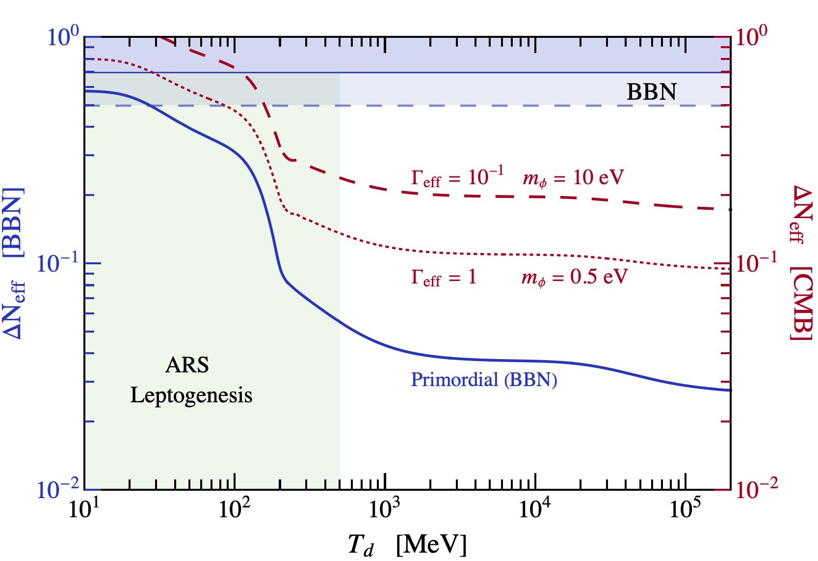
In the event that majoron decoupling is instantaneous, one can compute the energy density stored in the majoron population at BBN by simply accounting for the entropy dilution in the SM plasma after decoupling – this is shown in Fig. 2 (blue line labeled ‘Primordial’) as a function of decoupling temperature . Here, we express the energy density in terms of , where
| (20) |
and Escudero Abenza 2020; Akita and Yamaguchi 2020; Froustey et al. 2020; Bennett et al. 2020; Hansen et al. 2020.
It is worth noting that very light particles which decouple at extremely late times near MeV may be in tension with constraints from Big Bang Nucleosynthesis (BBN). There is, however, some ambiguity as to where these constraints truly lie; the reason being that the leading local cosmology-independent determinations of the primordial helium abundance rely on spectroscopic observations of HII in metal poor galaxies, which could suffer from systematics. The most recent estimate of is Aver et al. 2020: , but there are other independent analyses that report substantially larger values Izotov et al. 2014: . In order to account for the possibility of additional systematics in the determination of , we present throughout constraints on from these two distinct analyses – we defer a more detailed discussion of the BBN systematics and the sensitivity to to Appendix C. These constraints are plotted in Fig. 2 using horizontal blue lines (the excluded regions are shaded in blue, and differentiated using solid and dashed lines).
Should sterile neutrinos decay at , the effect of non-instantaneous majoron decoupling can lead to significant changes in the expected energy density of the primordial population. The reason here being simply that the SM plasma undergoes stronger and more rapid entropy dumps arising from the QCD phase transition. In order to more properly estimate the energy density in the parameter space of interest we have solved for the thermodynamic evolution of the and number densities in the early Universe, and evolved this system to temperatures for a wide array of sterile neutrino masses and interaction strengths. This was done using the methods of Escudero 2019; Escudero Abenza 2020, in which one assumes each population can be approximately described by a thermal distribution with a time-dependent temperature and chemical potential. Following this approach, we show the contribution to as a function of and in Fig. 3. We also highlight the preferred parameter space for the tension (red region). The details of this analysis are contained in Appendix B.

IV Majoron Cosmology
Having shown in the previous section that the same sterile neutrinos responsible for leptogenesis can also generate a sizable primordial population of majorons, we now turn our attention to the cosmological evolution of majorons after BBN. The story here is more straightforward: majorons with thermalize with neutrinos at temperatures via processes, and subsequently decay into neutrinos after becoming non-relativistic a short time later. There are two effects of this process: (1) a further increase in Escudero and Witte 2020; Chacko et al. 2004 and (2) a damping of the neutrino free streaming Bashinsky and Seljak 2004; Chacko et al. 2004. The former point has been illustrated in Fig. 2, where the contribution to at CMB (red) is compared for two different choices of parameters to the contribution to at BBN (blue). Assuming the majoron decays prior to recombination, models with lead to larger energy densities, as weakly coupled majorons remain non-relativistic for longer times before decaying. While the effect of damping neutrino free streaming is more subtle, these interactions can lead a noticeable imprint on the CMB multipoles. We outline our treatment of both of these effects in this section, and discuss the results of performing MCMCs to current cosmological data.
A. Background Evolution
In order to describe the background evolution of majorons and neutrinos in the early Universe we once again use the formalism developed in Escudero 2019; Escudero Abenza 2020 (described above). This was shown in Escudero Abenza 2020 to provide a highly accurate description of late-time thermalization of neutrinophilic bosons. We defer the details of these calculations to Appendix D.
Given an initial primordial majoron population characterized by , we can solve for the evolution for the neutrino-majoron system by accounting for majoron decays and inverse neutrino decays . Notice that this system is controlled by three parameters: the number of interacting neutrinos , the effective decay width given in Eq. (15), and the majoron mass. We highlight in Fig. 4 the impact of late-time neutrino-majoron thermalization on the expansion rate of the Universe (via the contribution to ), for various choices of these parameters. From the upper panel of Fig. 4 we can see that i) the presence of neutrino-majoron interactions enhances with respect to , and that ii) for the growth of is substantially larger (as mentioned above, this happens because for such values of majorons decay out of equilibrium at ). Finally, from the lower panel of Fig. 4 we can see the impact of accounting for the three possible values of . The results are fairly similar, but perhaps contrary to what could be expected, is larger for smaller . This happens simply as a result of equilibrium thermodynamics: smaller values of lead to a more degenerate final state population (because in practice more neutrinos have gone into that sector), and therefore have a larger energy density.

An enhancement of the expansion rate prior and close to recombination has long been appreciated as a key ingredient in models attempting to resolve the tension. The reason being that the characteristic angular size of fluctuations in the CMB has been measured with very high precision, Aghanim et al. 2020a. For a flat FLRW Universe, this angular scale can be written as
| (21) |
where represents the redshift of last scattering, is the photon-baryon sound speed, and is the expansion rate of the Universe. Given that is measured to such high precision, and that and are constrained via alternative observables, the most clear modification that allows for larger values of is to enhance prior to recombination Knox and Millea 2020. Using the approximate relationship between at recombination and derived in Vagnozzi 2020:
| (22) |
one can see that fully resolving the tension requires values of . The problem is that values of are disfavored by Planck data, regardless of whether this radiation is dark and free-streaming Aghanim et al. 2020a or strongly interacting Blinov and Marques-Tavares 2020. Our set up, however, is completely different from either of these cases because the majoron-neutrino interactions are only efficient for a limited period of time, roughly between . For the mass range of interest, this implies majoron-neutrino interactions will only alter CMB multipoles . This effect allows for an additional increase in relative to that of CDM without spoiling the fit to the Planck observations.
B. Planck Analysis
To study in detail the effect of majoron-neutrino perturbations on the CMB we have modified the cosmological Boltzmann code CLASS Blas et al. 2011; Lesgourgues 2011. In order to analyze the subsequent evolution of majorons as relevant for CMB observations we shall make a number of approximations, which we enumerate in what follows for the sake of clarity. First, we shall neglect neutrino masses in the evolution of the background energy density and at the level of the cosmological perturbations. We take this approximation because including neutrino masses at the perturbation level is rather complicated, see Barenboim et al. 2020. Nevertheless, this approximation is well justified provided that neutrino masses are at the level . This being said, large neutrino masses may be capable of reducing the value of , as was the case for the strongly interacting neutrino solution (see Kreisch et al. 2020). Second, for the purpose of describing the neutrino-majoron perturbations we assume that they form a single coupled fluid. This is a good approximation because all species are effectively relativistic except when the majorons decay. Their contribution to the equation of state of the system is always below for the models presented, and typically for the parameter space of interest55 5 This effect is larger for , which is why we choose not to display the results for this model. We note, however, that adopting this same assumption for the model yields posteriors that are nearly identical to the and 3 models.. Finally, we approximate the collision term at the perturbation level by the relaxation time approximation Hannestad and Scherrer 2000. This approach has been shown to be accurate for scenarios in which the interacting particles subtend large angles after collisions in the plasma Oldengott et al. 2017. In the parameter space we consider, majorons will only interact once they are mildly non-relativistic, by which time the typical angular separation of neutrinos in the cosmic frame is large, , which justifies our approach. Although it is beyond the scope of this paper to account for the exact collision term, we refer to Barenboim et al. 2020 for a recent study dealing with the exact collision term in the context of invisible neutrino decays.
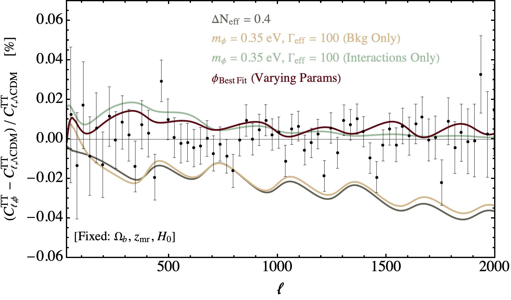
In Fig. 5 we show how the various effects described here effect the TT power spectrum. Specifically, we isolate each effect, and show the residuals relative to that of CDM for a majoron with eV and . These lines are produced by fixing , , and to their CDM values. We compare the background only contribution to a model in which is fixed to to illustrate that the late-time thermalization only effects low multipoles. We also show the best-fit majoron cosmology for and MeV in red (), which illustrates the high quality fit obtained from the MCMCs. From Fig. 5 we can appreciate that the neutrino-majoron interactions act as to partially cancel the background contribution at low multipoles.
To analyze in detail the cosmological implications of our scenario, we perform a MCMC using MontePython Audren et al. 2013; Brinckmann and Lesgourgues 2018 including only Planck2018+BAO data Aghanim et al. 2020a; Aghanim et al. 2020b66 6 Planck2018 data Aghanim et al. 2020a includes the high- and low- (temperature and polarization) and lensing likelihoods Aghanim et al. 2020b. In this work we use BAO data that includes the 6DF galaxy survey Beutler et al. 2011, the MGS galaxy sample of SDSS Ross et al. 2015, and the CMASS and LOWZ galaxy samples of BOSS DR12 Alam et al. 2017; Vargas-Magaña et al. 2018; Ross et al. 2017; Beutler et al. 2017, as used in the fiducial Planck analysis.77 7 We have also run an analysis including Pantheon type Ia supernova data, and have found that the preferred value of is surprisingly slightly shifted to yet higher values, and the with respect to LCDM is reduced. This emphasizes the robust nature of the obtained fit. . For each of our analyses we vary the standard cosmological parameters and nuisance parameters in the same way as the Planck collaboration in their legacy analysis Aghanim et al. 2020a. For the majoron mass and interaction we use log-scale priors with the following ranges88 8 We do not consider values because for such small interaction strengths majoron-neutrino interactions cannot significantly alter neutrino free-streaming. In addition, it was found that for models with a decoupling temperature MeV, larger priors on were needed, and thus in these cases we adopt a log flat prior over the range . :
| (23) | ||||
| (24) |
We note that the lower limit on is imposed on the physicality of our model. It corresponds to the minimal mass for which the majoron can decay into the most massive neutrino . For smaller masses the majoron could potentially participate in the process of neutrino decay leading to a very different phenomenology Barenboim et al. 2020; Escudero et al. 2020; Chacko et al. 2020; Chacko et al. 2021; Escudero and Fairbairn 2019; Hannestad and Raffelt 2005. This, however, will in fact not occur within the framework of the singlet majoron model considered here, see Schechter and Valle 1982.
In our runs we do not vary the initial primordial majoron population, i.e. or equivalently , but instead we explore some representative values expected to arise from low-scale leptogenesis; this is because of the difficulty in computing the thermodynamic evolution on-the-fly, something the authors hope to improve upon in future work. We also explore scenarios with interacting neutrino species. Nevertheless, in what follows, we concentrate on for concreteness because our runs show that the posteriors are fairly independent of whether .
In Fig. 6 we show the resulting posterior (see Appendix D for the full results) for analyses with and in green, and CDM in grey. For comparison, we also plot the one and two sigma posterior from local measurements of performed by the SH0ES collaboration, which find km/s/Mpc Riess et al. 2021.
From our analysis of the fiducial model we obtain a number of relevant results:
- 1.
Majoron cosmologies with a primordial population at the level of lead to substantially larger values of than CDM:
(25) - 2.
With respect to CDM, there are upward shifts on other cosmological parameters such as , , and . Importantly, the observed shift in the preferred value of is in agreement with observations from BBN (see Appendix C for additional details).
- 3.
The majoron mass needed to obtain these rather large values of is bounded from above to be:
(26) and is bounded from below at . We note that these masses are in agreement with the expectations from Fig. 4. In addition, we note that this upper limit highlights that primordial populations of majorons with larger than eV-scale masses that decay well before recombination are not favored by Planck legacy data.
- 4.
The preferred region of parameter space for majoron interactions is
(27) - 5.
The Planck legacy data points to scales of spontaneous lepton number breaking:
(28) where this number is obtained by taking Eq. (10) with , but we note that the bound on could be as large as TeV for more massive neutrinos.
- 6.
The best-fit point for of the fiducial model has a of:
(29) and corresponds to
(30) These values highlight that for moderately large the fit to Planck+BAO data can be improved relative to CDM. However, our other analyses show that the fit becomes degraded for primordial populations with . Notice that these values of are excluded at more than 2 if the damping of neutrino free streaming is not included Aghanim et al. 2020a.

C. Implication for the Hubble Tension
In order to determine the significance with which the leptogenesis motivated majoron resolves the Hubble tension, we use the so-called posterior predictive distribution Gelman et al. 2013 (PPD) as proposed in Feeney et al. 2019. Simply put, the idea is to determine the distribution of expected measurements obtained from new data given a set of observed data and a model ; in the context of the Hubble tension, this is equivalent to asking the question: given the value of observed by CMB and BAO data within a particular cosmology (taken here to be either CDM or the primordial majoron cosmology), how likely is it for the SH0ES collaboration to measure some other value ? The PPD is obtained by averaging the likelihood of the new data over the posterior of the parameters of the existing data, i.e.
| (31) |
Importantly, there is no assumption that the two datasets under consideration are consistent. Rather, the PPD allows one to determine whether the second dataset is a likely draw from the first. We apply this method using the measurement of by the SH0ES collaboration, for which we adopt a Gaussian likelihood with central value km/s/Mpc and uncertainty km/s/Mpc Riess et al. 2021. We plot the PPD for CDM and the leptogenesis-inspired majoron model with in Fig. 7 (shaded regions). The central value of the SH0ES measurement is also shown for comparison (vertical yellow line).
The potential tension between the CMB+BAO measurement and that of SH0ES can then be obtained using the PPD ratio, defined as
| (32) |
where is the value of the Hubble constant observed by SH0ES by using the Cepheid Distance Ladder (CDL). The PPD ratio can be interpreted as a lower bound on posterior probability of the hypothesis that the CMB+BAO data and that of SH0ES arise from the same value of without unaccounted for systematics. In the case of CDM, we find a value of , implying the probability that the SH0ES measurement is unaffected by systematics and appears only from statistical fluctuations, is roughly . In the majoron model, on the other hand, we find a value of . Admittedly, this metric does not account for the fact that additional model parameters have been introduced; nevertheless, the statistical tension between these datasets in the context of CDM is sufficiently large that novel physics must now be considered, and thus it is perhaps more appropriate to compare the number of model parameters introduced only between proposed solutions to the Hubble tension.
A potential criticism of this treatment is that the decoupling temperature is fixed, rather than scanned, and thus has preferentially selected a large value of 99 9 Note that implementing a scan of is quite complicated and time consuming, as the out-of-equilibrium evolution of the majoron must be solved on the fly in CLASS Blas et al. 2011; Lesgourgues 2011. ; the current treatment can be interpreted as adopting a strong prior on the ARS leptogenesis-motivated decoupling temperature. As shown in Appendix D, the of the best-fit is approximately equivalent to, and actually slightly below, that of CDM. It is thus straightforward to understand that the effect of scanning would simply be to broaden the posterior on about a value of km/s/Mpc, extending at lower values to what is found in CDM1010 10 The limit in which , , and is as close as this model can be to recovering CDM, however even in this limit energy is injected at the level of . and potentially extending in the low decoupling temperature limit to a value km/s/Mpc (as shown in Escudero and Witte 2020). Including a prior on from e.g. the SH0ES measurement, however, would shift the posterior to values of larger than that obtained here, and remove the part of the posterior near the CDM value.
V Summary and Conclusions
Majorons with masses can thermalize with neutrinos prior and close to recombination, damping neutrino free streaming, altering the energy density stored in the neutrinos themselves. These effects manifest in the CMB power spectrum in a manner that partially cancels, however there is a residual scale-dependent phase shift that leads to a preference for larger values of , , and . This motivated the authors’ previous study Escudero and Witte 2020, where it was shown that a majoron with a mass arising from a the spontaneous breaking of a lepton number symmetry at scales TeV could reduce the Hubble tension to the level, however only if additional dark radiation was present at the level of .
In this work we have investigated the extent to which a primordial population of majorons arising from low-scale models of leptogenesis can source the additional radiation required to ameliorate the tension. We have found that so long as the Higgs’ portal coupling is sufficiently small () so as to avoid thermalizing the new scalars at high temperatures and that the lepton number phase transition occurs at , ARS leptogenesis in the singlet majoron model will proceed as normal. Given the sterile neutrino masses required for ARS leptogensis and the range of interaction strengths required for majorons to thermalize at late times, sterile neutrinos will inevitably create a thermal majoron population at temperatures . This primordial majoron population will eventually decouple as sterile neutrinos decay , naturally sourcing a contribution of (at BBN), see Fig. 3. Given that a large population of primordial majorons can be produced in the early Universe, the question becomes whether the late-time evolution of the majoron-neutrino system behaves similarly to the analysis of Escudero and Witte 2020 (since the time-dependence of the interaction rate has been modified), and whether the result is sensitive to the number of interacting neutrinos. Our results indicate that all three scenarios (i.e. that in which one, two, or all three neutrinos interact) favor similar parameter space, provide a similar shift in , and yield comparable values to CMB and BAO data. The preferred value of of these models using only Planck2018+BAO data is found to be km/s/Mpc, still below the value reported by the SH0ES collaboration km/s/Mpc Riess et al. 2021, but compatible at the level (to be compared with in CDM). It remains to be seen whether a more robust analysis including non-zero neutrino masses, both in the evolution of the background and at the level of the perturbations, would alter the results in a significant manner.
To summarize, we have shown that the Hubble tension could be a signal of low-scale leptogenesis and neutrino mass generation within a simple and well-motivated neutrino mass model. In this set up, lepton number is a global symmetry that is spontaneously broken at an energy scale . This generates Majorana masses for sterile neutrinos, which in turn via the type-I seesaw lead to an understanding of the small neutrino masses. In addition, upon breaking of a pseudo-Goldstone boson appears on the spectrum, the majoron . This particle is naturally very light and eV masses for it are motivated from Planck-scale suppressed operators that explicitly break lepton number, . Furthermore, in this set up, the interactions between neutrinos and majorons are extremely feeble, . Intriguingly, these very small couplings and masses precisely correspond to processes turning on right before recombination for . Indeed, our Planck legacy data analysis shows that the preferred region of parameter space within a primordial majoron cosmology is:
| (33) | ||||
| (34) | ||||
| (35) |
which point towards
| (36) |
Finally, given that the preferred scale of lepton number breaking is this naturally points to GeV-scale sterile neutrinos. In particular, these sterile neutrinos can produce the right primordial majoron population (see Fig. 3) and also generate via their oscillations the sufficient leptonic CP asymmetry in the early Universe. Therefore providing an understanding of the observed asymmetry between matter and antimatter.
VI Outlook
We have presented a connection between the Hubble tension, leptogenesis and the origin of neutrino masses. In what follows, we enumerate a list of aspects that fall beyond the scope of this study but that we believe deserve future attention:
- 1.
Refined cosmological analysis. As discussed in the main text, we have made three approximations which simplify the treatment of the majoron cosmology: i) We have neglected the effect of neutrino masses in the evolution of both the background and the perturbations of the Universe. This is well-justified for as Planck CMB observations are not sensitive to such small neutrino masses. However, an actual analysis could potentially reveal the preference of higher neutrino masses which will yield a smaller value of as relevant for weak lensing measurements of this parameter, see e.g. Jedamzik et al. 2020. ii) We have modeled the majoron-neutrino perturbations by making use of the relaxation time approximation for the collision term. As argued in Section IV we believe that this should be a good approximation because in our parameter space of interest majorons interact with neutrinos once they become mildly non-relativistic, implying that the final state particles will be roughly isotropically produced (as assumed by the relaxation approximation to capture the effect on the anisotropic stress). It would, however, be very interesting to explore the phenomenology accounting for the exact collision term. iii) We have treated the neutrino-majoron system as a single coupled fluid. While this assumption holds in the relativistic limit, the isotropisation of the fluid decreases as majorons become non-relativistic and decay. It is thus possible that relaxing this assumption, and properly incorporating the decay hierarchy, could potentially reduce the maximum allowed value of . We hope to refine this treatment, and properly assess the importance of this effect, in future work.
- 2.
ARS Leptogenesis in the singlet majoron model. In this work (see also Caputo et al. 2019) we have derived a minimal set of conditions necessary for the singlet majoron model not to spoil successful ARS leptogenesis. In order to robustly determine the parameter space of interest more rigorous calculations would be necessary1111 11 We note that baryogenesis/leptogenesis has been explored in the majoron model in the context of electroweak baryogenesis Cohen et al. 1991; Cohen et al. 1990, thermal leptogenesis Aristizabal Sierra et al. 2014, and resonant leptogenesis Pilaftsis 2008. In addition, we note that the CP violating decays of Higgs doublets into sterile neutrinos in the early Universe can yield relevant lepton asymmetries that could (depending upon the mass degeneracy) dominate over the contribution arising from oscillations Hambye and Teresi 2016; Hambye and Teresi 2017.. We note that given the temperature dependence of is this model, such analysis may yield even more favorable conditions for the production of a lepton asymmetry from sterile neutrino oscillations.
- 3.
Collider Detectability. Although in this study we have exhausted the cosmological implications of majorons and their companion neutrinos and sterile neutrinos, we have not discussed potential signals at laboratory experiments. From the collider perspective, it appears quite difficult to test the scalar sector of the theory given the smallness of the Higgs portal coupling and the smallness of the neutrino-majoron couplings. However, in the context of sterile neutrinos there are some possibilities. In our set up, sterile neutrinos decay invisibly into a neutrino and a majoron (see Eq. (13)). This means that typical searches at beam-dump experiments (see e.g. Alekhin et al. 2016) will not have sensitivity to this model. The best avenue to detect these GeV-scale sterile neutrinos may be to look for Aguilar-Arevalo et al. 2018; Cortina Gil et al. 2021 decays, where the particles appears in the form of missing energy. While at the moment current experiments are sensitive to active-sterile neutrino mixings orders of magnitude larger than in the naive seesaw limit (see Eq. (5)), ongoing and upcoming experiments looking for these decays Beacham et al. 2020 may be sensitive to the minimum mixing expected from the seesaw for .
In this work we have shown that the Hubble tension can be largely ameliorated in a simple framework that explains both the origin of the active neutrino masses (via the seesaw mechanism) and the baryon asymmetry of the Universe (via the ARS leptogenesis mechanism). This proposal may be exhaustively tested by both future cosmological observations and by looking in terrestrial experiments for the presence of GeV-scale sterile neutrinos, which are necessary to source both the primordial majoron population and a primordial lepton asymmetry.
Acknowledgments
We are grateful to Iván Esteban, Pilar Hernández, Kevin Kelly, Manuel Masip, Vivian Poulin, Nuria Rius and Jordi Salvadó for very useful comments and discussions. ME is supported by a Fellowship of the Alexander von Humboldt Foundation. SJW acknowledges funding from the European Research Council (ERC) under the European Union’s Horizon 2020 research and innovation programme (Grant agreement No. 864035 - UnDark).
References
- Aghanim et al. (2020a) N. Aghanim et al. (Planck), Astron. Astrophys. 641, A6 (2020a), arXiv:1807.06209 [astro-ph.CO] .
- Aghanim et al. (2020b) N. Aghanim et al. (Planck), Astron. Astrophys. 641, A5 (2020b), arXiv:1907.12875 [astro-ph.CO] .
- Abbott et al. (2018) T. M. C. Abbott et al. (DES), Mon. Not. Roy. Astron. Soc. 480, 3879 (2018), arXiv:1711.00403 [astro-ph.CO] .
- Addison et al. (2018) G. E. Addison, D. J. Watts, C. L. Bennett, M. Halpern, G. Hinshaw, and J. L. Weiland, Astrophys. J. 853, 119 (2018), arXiv:1707.06547 [astro-ph.CO] .
- Schöneberg et al. (2019) N. Schöneberg, J. Lesgourgues, and D. C. Hooper, JCAP 10, 029 (2019), arXiv:1907.11594 [astro-ph.CO] .
- Cuceu et al. (2019) A. Cuceu, J. Farr, P. Lemos, and A. Font-Ribera, JCAP 10, 044 (2019), arXiv:1906.11628 [astro-ph.CO] .
- Riess et al. (2016) A. G. Riess et al., Astrophys. J. 826, 56 (2016), arXiv:1604.01424 [astro-ph.CO] .
- Riess et al. (2019) A. G. Riess, S. Casertano, W. Yuan, L. M. Macri, and D. Scolnic, Astrophys. J. 876, 85 (2019), arXiv:1903.07603 [astro-ph.CO] .
- Dhawan et al. (2018) S. Dhawan, S. W. Jha, and B. Leibundgut, Astron. Astrophys. 609, A72 (2018), arXiv:1707.00715 [astro-ph.CO] .
- Burns et al. (2018) C. R. Burns et al. (CSP), Astrophys. J. 869, 56 (2018), arXiv:1809.06381 [astro-ph.CO] .
- Riess et al. (2018) A. G. Riess et al., Astrophys. J. 855, 136 (2018), arXiv:1801.01120 [astro-ph.SR] .
- Freedman et al. (2019) W. L. Freedman et al., Astrophys. J. 882, 34 (2019), arXiv:1907.05922 [astro-ph.CO] .
- Yuan et al. (2019) W. Yuan, A. G. Riess, L. M. Macri, S. Casertano, and D. Scolnic, Astrophys. J. 886, 61 (2019), arXiv:1908.00993 [astro-ph.GA] .
- Reid et al. (2019) M. J. Reid, D. W. Pesce, and A. G. Riess, Astrophys. J. Lett. 886, L27 (2019), arXiv:1908.05625 [astro-ph.GA] .
- Riess et al. (2021) A. G. Riess, S. Casertano, W. Yuan, J. B. Bowers, L. Macri, J. C. Zinn, and D. Scolnic, Astrophys. J. Lett. 908, L6 (2021), arXiv:2012.08534 [astro-ph.CO] .
- Bonvin et al. (2017) V. Bonvin et al., Mon. Not. Roy. Astron. Soc. 465, 4914 (2017), arXiv:1607.01790 [astro-ph.CO] .
- Birrer et al. (2019) S. Birrer et al., Mon. Not. Roy. Astron. Soc. 484, 4726 (2019), arXiv:1809.01274 [astro-ph.CO] .
- Rusu et al. (2020) C. E. Rusu et al., Mon. Not. Roy. Astron. Soc. 498, 1440 (2020), arXiv:1905.09338 [astro-ph.CO] .
- Chen et al. (2019) G. C. F. Chen et al., Mon. Not. Roy. Astron. Soc. 490, 1743 (2019), arXiv:1907.02533 [astro-ph.CO] .
- Wong et al. (2020) K. C. Wong et al., Mon. Not. Roy. Astron. Soc. 498, 1420 (2020), arXiv:1907.04869 [astro-ph.CO] .
- Blakeslee et al. (2021) J. P. Blakeslee, J. B. Jensen, C.-P. Ma, P. A. Milne, and J. E. Greene, (2021), arXiv:2101.02221 [astro-ph.CO] .
- Reid et al. (2009) M. Reid, J. Braatz, J. Condon, L. Greenhill, C. Henkel, and K. Lo, Astrophys. J. 695, 287 (2009), arXiv:0811.4345 [astro-ph] .
- Verde et al. (2019) L. Verde, T. Treu, and A. G. Riess (2019) arXiv:1907.10625 [astro-ph.CO] .
- Riess (2019) A. G. Riess, Nature Rev. Phys. 2, 10 (2019), arXiv:2001.03624 [astro-ph.CO] .
- Martsell and Dhawan (2018) E. Martsell and S. Dhawan, JCAP 1809, 025 (2018), arXiv:1801.07260 [astro-ph.CO] .
- Poulin et al. (2018) V. Poulin, K. K. Boddy, S. Bird, and M. Kamionkowski, Phys. Rev. D 97, 123504 (2018), arXiv:1803.02474 [astro-ph.CO] .
- Nunes (2018) R. C. Nunes, JCAP 05, 052 (2018), arXiv:1802.02281 [gr-qc] .
- Di Valentino et al. (2020) E. Di Valentino, A. Melchiorri, O. Mena, and S. Vagnozzi, Phys. Dark Univ. 30, 100666 (2020), arXiv:1908.04281 [astro-ph.CO] .
- Vattis et al. (2019) K. Vattis, S. M. Koushiappas, and A. Loeb, Phys. Rev. D 99, 121302 (2019), arXiv:1903.06220 [astro-ph.CO] .
- Li et al. (2019) X. Li, A. Shafieloo, V. Sahni, and A. A. Starobinsky, Astrophys. J. 887, 153 (2019), arXiv:1904.03790 [astro-ph.CO] .
- Visinelli et al. (2019) L. Visinelli, S. Vagnozzi, and U. Danielsson, Symmetry 11, 1035 (2019), arXiv:1907.07953 [astro-ph.CO] .
- Yang et al. (2021) W. Yang, E. Di Valentino, S. Pan, and O. Mena, Phys. Dark Univ. 31, 100762 (2021), arXiv:2007.02927 [astro-ph.CO] .
- Poulin et al. (2019) V. Poulin, T. L. Smith, T. Karwal, and M. Kamionkowski, Phys. Rev. Lett. 122, 221301 (2019), arXiv:1811.04083 [astro-ph.CO] .
- Agrawal et al. (2019) P. Agrawal, F.-Y. Cyr-Racine, D. Pinner, and L. Randall, (2019), arXiv:1904.01016 [astro-ph.CO] .
- Lin et al. (2019) M.-X. Lin, G. Benevento, W. Hu, and M. Raveri, Phys. Rev. D 100, 063542 (2019), arXiv:1905.12618 [astro-ph.CO] .
- Smith et al. (2020) T. L. Smith, V. Poulin, and M. A. Amin, Phys. Rev. D 101, 063523 (2020), arXiv:1908.06995 [astro-ph.CO] .
- D’Eramo et al. (2018) F. D’Eramo, R. Z. Ferreira, A. Notari, and J. L. Bernal, JCAP 1811, 014 (2018), arXiv:1808.07430 [hep-ph] .
- Escudero et al. (2019) M. Escudero, D. Hooper, G. Krnjaic, and M. Pierre, JHEP 03, 071 (2019), arXiv:1901.02010 [hep-ph] .
- Bringmann et al. (2018) T. Bringmann, F. Kahlhoefer, K. Schmidt-Hoberg, and P. Walia, Phys. Rev. D98, 023543 (2018), arXiv:1803.03644 [astro-ph.CO] .
- Pandey et al. (2020) K. L. Pandey, T. Karwal, and S. Das, JCAP 07, 026 (2020), arXiv:1902.10636 [astro-ph.CO] .
- Blinov et al. (2020) N. Blinov, C. Keith, and D. Hooper, JCAP 06, 005 (2020), arXiv:2004.06114 [astro-ph.CO] .
- Blinov and Marques-Tavares (2020) N. Blinov and G. Marques-Tavares, JCAP 09, 029 (2020), arXiv:2003.08387 [astro-ph.CO] .
- Lancaster et al. (2017) L. Lancaster, F.-Y. Cyr-Racine, L. Knox, and Z. Pan, JCAP 1707, 033 (2017), arXiv:1704.06657 [astro-ph.CO] .
- Kreisch et al. (2020) C. D. Kreisch, F.-Y. Cyr-Racine, and O. Doré, Phys. Rev. D 101, 123505 (2020), arXiv:1902.00534 [astro-ph.CO] .
- Park et al. (2019) M. Park, C. D. Kreisch, J. Dunkley, B. Hadzhiyska, and F.-Y. Cyr-Racine, Phys. Rev. D 100, 063524 (2019), arXiv:1904.02625 [astro-ph.CO] .
- Sakstein and Trodden (2020) J. Sakstein and M. Trodden, Phys. Rev. Lett. 124, 161301 (2020), arXiv:1911.11760 [astro-ph.CO] .
- Archidiacono et al. (2020) M. Archidiacono, S. Gariazzo, C. Giunti, S. Hannestad, and T. Tram, JCAP 12, 029 (2020), arXiv:2006.12885 [astro-ph.CO] .
- Choi et al. (2020) G. Choi, M. Suzuki, and T. T. Yanagida, Phys. Rev. D 101, 075031 (2020), arXiv:2002.00036 [hep-ph] .
- Freese and Winkler (2021) K. Freese and M. W. Winkler, (2021), arXiv:2102.13655 [astro-ph.CO] .
- Di Valentino et al. (2021) E. Di Valentino, O. Mena, S. Pan, L. Visinelli, W. Yang, A. Melchiorri, D. F. Mota, A. G. Riess, and J. Silk, (2021), arXiv:2103.01183 [astro-ph.CO] .
- Bernal et al. (2016) J. L. Bernal, L. Verde, and A. G. Riess, JCAP 1610, 019 (2016), arXiv:1607.05617 [astro-ph.CO] .
- Aylor et al. (2019) K. Aylor, M. Joy, L. Knox, M. Millea, S. Raghunathan, and W. K. Wu, Astrophys. J. 874, 4 (2019), arXiv:1811.00537 [astro-ph.CO] .
- Knox and Millea (2020) L. Knox and M. Millea, Phys. Rev. D 101, 043533 (2020), arXiv:1908.03663 [astro-ph.CO] .
- Escudero and Witte (2020) M. Escudero and S. J. Witte, Eur. Phys. J. C 80, 294 (2020), arXiv:1909.04044 [astro-ph.CO] .
- Escudero Abenza and Witte (2020) M. Escudero Abenza and S. J. Witte, in Prospects in Neutrino Physics, NuPhys2019 (2020) arXiv:2004.01470 [hep-ph] .
- Chikashige et al. (1981) Y. Chikashige, R. N. Mohapatra, and R. D. Peccei, Phys. Lett. 98B, 265 (1981).
- Gelmini and Roncadelli (1981) G. B. Gelmini and M. Roncadelli, Phys. Lett. 99B, 411 (1981).
- Georgi et al. (1981) H. M. Georgi, S. L. Glashow, and S. Nussinov, Nucl. Phys. B193, 297 (1981).
- Schechter and Valle (1982) J. Schechter and J. W. F. Valle, Phys. Rev. D25, 774 (1982).
- Chacko et al. (2004) Z. Chacko, L. J. Hall, T. Okui, and S. J. Oliver, Phys. Rev. D70, 085008 (2004), arXiv:hep-ph/0312267 [hep-ph] .
- Bashinsky and Seljak (2004) S. Bashinsky and U. Seljak, Phys. Rev. D69, 083002 (2004), arXiv:astro-ph/0310198 [astro-ph] .
- Rothstein et al. (1993) I. Z. Rothstein, K. S. Babu, and D. Seckel, Nucl. Phys. B403, 725 (1993), arXiv:hep-ph/9301213 [hep-ph] .
- Akhmedov et al. (1993) E. K. Akhmedov, Z. G. Berezhiani, R. N. Mohapatra, and G. Senjanovic, Phys. Lett. B299, 90 (1993), arXiv:hep-ph/9209285 [hep-ph] .
- Kallosh et al. (1995) R. Kallosh, A. D. Linde, D. A. Linde, and L. Susskind, Phys. Rev. D52, 912 (1995), arXiv:hep-th/9502069 [hep-th] .
- Banks and Seiberg (2011) T. Banks and N. Seiberg, Phys. Rev. D83, 084019 (2011), arXiv:1011.5120 [hep-th] .
- Witten (2018) E. Witten, Nature Phys. 14, 116 (2018), arXiv:1710.01791 [hep-th] .
- Harlow and Ooguri (2019) D. Harlow and H. Ooguri, Phys. Rev. Lett. 122, 191601 (2019), arXiv:1810.05337 [hep-th] .
- Fichet and Saraswat (2020) S. Fichet and P. Saraswat, JHEP 01, 088 (2020), arXiv:1909.02002 [hep-th] .
- Alvey and Escudero (2021) J. Alvey and M. Escudero, JHEP 01, 032 (2021), arXiv:2009.03917 [hep-ph] .
- Blinov et al. (2019) N. Blinov, K. J. Kelly, G. Z. Krnjaic, and S. D. McDermott, Phys. Rev. Lett. 123, 191102 (2019), arXiv:1905.02727 [astro-ph.CO] .
- Lyu et al. (2021) K.-F. Lyu, E. Stamou, and L.-T. Wang, Phys. Rev. D 103, 015004 (2021), arXiv:2004.10868 [hep-ph] .
- Brdar et al. (2020) V. Brdar, M. Lindner, S. Vogl, and X.-J. Xu, Phys. Rev. D 101, 115001 (2020), arXiv:2003.05339 [hep-ph] .
- Pitrou et al. (2018) C. Pitrou, A. Coc, J.-P. Uzan, and E. Vangioni, Phys. Rept. 754, 1 (2018), arXiv:1801.08023 [astro-ph.CO] .
- Fields et al. (2020) B. D. Fields, K. A. Olive, T.-H. Yeh, and C. Young, JCAP 03, 010 (2020), arXiv:1912.01132 [astro-ph.CO] .
- Huang and Rodejohann (2021) G.-y. Huang and W. Rodejohann, (2021), arXiv:2102.04280 [hep-ph] .
- Seto and Toda (2021) O. Seto and Y. Toda, (2021), arXiv:2101.03740 [astro-ph.CO] .
- Berbig et al. (2020) M. Berbig, S. Jana, and A. Trautner, Phys. Rev. D 102, 115008 (2020), arXiv:2004.13039 [hep-ph] .
- He et al. (2020) H.-J. He, Y.-Z. Ma, and J. Zheng, JCAP 11, 003 (2020), arXiv:2003.12057 [hep-ph] .
- Roy Choudhury et al. (2020) S. Roy Choudhury, S. Hannestad, and T. Tram, (2020), arXiv:2012.07519 [astro-ph.CO] .
- Das and Ghosh (2020) A. Das and S. Ghosh, (2020), arXiv:2011.12315 [hep-ph] .
- Brinckmann et al. (2020) T. Brinckmann, J. H. Chang, and M. LoVerde, (2020), arXiv:2012.11830 [astro-ph.CO] .
- Akhmedov et al. (1998) E. K. Akhmedov, V. Rubakov, and A. Smirnov, Phys. Rev. Lett. 81, 1359 (1998), arXiv:hep-ph/9803255 .
- Asaka and Shaposhnikov (2005) T. Asaka and M. Shaposhnikov, Phys. Lett. B 620, 17 (2005), arXiv:hep-ph/0505013 .
- Shaposhnikov (2008) M. Shaposhnikov, JHEP 08, 008 (2008), arXiv:0804.4542 [hep-ph] .
- Drewes et al. (2018) M. Drewes, B. Garbrecht, P. Hernandez, M. Kekic, J. Lopez-Pavon, J. Racker, N. Rius, J. Salvado, and D. Teresi, Int. J. Mod. Phys. A 33, 1842002 (2018), arXiv:1711.02862 [hep-ph] .
- Vilenkin and Everett (1982) A. Vilenkin and A. Everett, Phys. Rev. Lett. 48, 1867 (1982).
- Kawasaki and Nakayama (2013) M. Kawasaki and K. Nakayama, Ann. Rev. Nucl. Part. Sci. 63, 69 (2013), arXiv:1301.1123 [hep-ph] .
- Minkowski (1977) P. Minkowski, Phys. Lett. 67B, 421 (1977).
- Mohapatra and Senjanovic (1981) R. N. Mohapatra and G. Senjanovic, Phys. Rev. D23, 165 (1981).
- Gell-Mann et al. (1979) M. Gell-Mann, P. Ramond, and R. Slansky, Supergravity Workshop Stony Brook, New York, September 27-28, 1979, Conf. Proc. C790927, 315 (1979), arXiv:1306.4669 [hep-th] .
- Yanagida (1980) T. Yanagida, Prog. Theor. Phys. 64, 1103 (1980).
- Schechter and Valle (1980) J. Schechter and J. Valle, Phys. Rev. D 22, 2227 (1980).
- Casas and Ibarra (2001) J. Casas and A. Ibarra, Nucl. Phys. B 618, 171 (2001), arXiv:hep-ph/0103065 .
- Arias-Aragon et al. (2021) F. Arias-Aragon, E. Fernandez-Martinez, M. Gonzalez-Lopez, and L. Merlo, Eur. Phys. J. C 81, 28 (2021), arXiv:2009.01848 [hep-ph] .
- Pilaftsis (1992) A. Pilaftsis, Z. Phys. C 55, 275 (1992), arXiv:hep-ph/9901206 .
- Pilaftsis (1994) A. Pilaftsis, Phys. Rev. D 49, 2398 (1994), arXiv:hep-ph/9308258 .
- Gonzalez-Garcia et al. (1990) M. Gonzalez-Garcia, A. Santamaria, and J. Valle, Nucl. Phys. B 342, 108 (1990).
- Esteban et al. (2020) I. Esteban, M. Gonzalez-Garcia, M. Maltoni, T. Schwetz, and A. Zhou, JHEP 09, 178 (2020), arXiv:2007.14792 [hep-ph] .
- de Salas et al. (2020) P. de Salas, D. Forero, S. Gariazzo, P. Martínez-Miravé, O. Mena, C. Ternes, M. Tórtola, and J. Valle, (2020), arXiv:2006.11237 [hep-ph] .
- Hernández et al. (2015) P. Hernández, M. Kekic, J. López-Pavón, J. Racker, and N. Rius, JHEP 10, 067 (2015), arXiv:1508.03676 [hep-ph] .
- Hernández et al. (2016) P. Hernández, M. Kekic, J. López-Pavón, J. Racker, and J. Salvado, JHEP 08, 157 (2016), arXiv:1606.06719 [hep-ph] .
- Eijima et al. (2019) S. Eijima, M. Shaposhnikov, and I. Timiryasov, JHEP 07, 077 (2019), arXiv:1808.10833 [hep-ph] .
- Klarić et al. (2020) J. Klarić, M. Shaposhnikov, and I. Timiryasov, (2020), arXiv:2008.13771 [hep-ph] .
- Drewes and Garbrecht (2013) M. Drewes and B. Garbrecht, JHEP 03, 096 (2013), arXiv:1206.5537 [hep-ph] .
- Caputo et al. (2019) A. Caputo, P. Hernandez, and N. Rius, Eur. Phys. J. C 79, 574 (2019), arXiv:1807.03309 [hep-ph] .
- Staub (2008) F. Staub, (2008), arXiv:0806.0538 [hep-ph] .
- Staub (2015) F. Staub, Adv. High Energy Phys. 2015, 840780 (2015), arXiv:1503.04200 [hep-ph] .
- Laine and Meyer (2015) M. Laine and M. Meyer, JCAP 07, 035 (2015), arXiv:1503.04935 [hep-ph] .
- Izotov et al. (2014) Y. I. Izotov, T. X. Thuan, and N. G. Guseva, Mon. Not. Roy. Astron. Soc. 445, 778 (2014), arXiv:1408.6953 [astro-ph.CO] .
- Aver et al. (2020) E. Aver, D. A. Berg, K. A. Olive, R. W. Pogge, J. J. Salzer, and E. D. Skillman, (2020), arXiv:2010.04180 [astro-ph.CO] .
- Ghiglieri and Laine (2016) J. Ghiglieri and M. Laine, JCAP 07, 015 (2016), arXiv:1605.07720 [hep-ph] .
- Escudero Abenza (2020) M. Escudero Abenza, JCAP 05, 048 (2020), arXiv:2001.04466 [hep-ph] .
- Akita and Yamaguchi (2020) K. Akita and M. Yamaguchi, JCAP 08, 012 (2020), arXiv:2005.07047 [hep-ph] .
- Froustey et al. (2020) J. Froustey, C. Pitrou, and M. C. Volpe, JCAP 12, 015 (2020), arXiv:2008.01074 [hep-ph] .
- Bennett et al. (2020) J. J. Bennett, G. Buldgen, P. F. de Salas, M. Drewes, S. Gariazzo, S. Pastor, and Y. Y. Y. Wong, (2020), arXiv:2012.02726 [hep-ph] .
- Hansen et al. (2020) R. S. L. Hansen, S. Shalgar, and I. Tamborra, (2020), arXiv:2012.03948 [astro-ph.CO] .
- Escudero (2019) M. Escudero, JCAP 1902, 007 (2019), arXiv:1812.05605 [hep-ph] .
- Vagnozzi (2020) S. Vagnozzi, Phys. Rev. D 102, 023518 (2020), arXiv:1907.07569 [astro-ph.CO] .
- Blas et al. (2011) D. Blas, J. Lesgourgues, and T. Tram, JCAP 1107, 034 (2011), arXiv:1104.2933 [astro-ph.CO] .
- Lesgourgues (2011) J. Lesgourgues, (2011), arXiv:1104.2932 [astro-ph.IM] .
- Barenboim et al. (2020) G. Barenboim, J. Z. Chen, S. Hannestad, I. M. Oldengott, T. Tram, and Y. Y. Y. Wong, (2020), arXiv:2011.01502 [astro-ph.CO] .
- Hannestad and Scherrer (2000) S. Hannestad and R. J. Scherrer, Phys. Rev. D 62, 043522 (2000), arXiv:astro-ph/0003046 .
- Oldengott et al. (2017) I. M. Oldengott, T. Tram, C. Rampf, and Y. Y. Y. Wong, JCAP 11, 027 (2017), arXiv:1706.02123 [astro-ph.CO] .
- Audren et al. (2013) B. Audren, J. Lesgourgues, K. Benabed, and S. Prunet, JCAP 1302, 001 (2013), arXiv:1210.7183 [astro-ph.CO] .
- Brinckmann and Lesgourgues (2018) T. Brinckmann and J. Lesgourgues, (2018), arXiv:1804.07261 [astro-ph.CO] .
- Beutler et al. (2011) F. Beutler, C. Blake, M. Colless, D. H. Jones, L. Staveley-Smith, L. Campbell, Q. Parker, W. Saunders, and F. Watson, Mon. Not. Roy. Astron. Soc. 416, 3017 (2011), arXiv:1106.3366 [astro-ph.CO] .
- Ross et al. (2015) A. J. Ross, L. Samushia, C. Howlett, W. J. Percival, A. Burden, and M. Manera, Mon. Not. Roy. Astron. Soc. 449, 835 (2015), arXiv:1409.3242 [astro-ph.CO] .
- Alam et al. (2017) S. Alam et al. (BOSS), Mon. Not. Roy. Astron. Soc. 470, 2617 (2017), arXiv:1607.03155 [astro-ph.CO] .
- Vargas-Magaña et al. (2018) M. Vargas-Magaña et al., Mon. Not. Roy. Astron. Soc. 477, 1153 (2018), arXiv:1610.03506 [astro-ph.CO] .
- Ross et al. (2017) A. J. Ross et al. (BOSS), Mon. Not. Roy. Astron. Soc. 464, 1168 (2017), arXiv:1607.03145 [astro-ph.CO] .
- Beutler et al. (2017) F. Beutler et al. (BOSS), Mon. Not. Roy. Astron. Soc. 464, 3409 (2017), arXiv:1607.03149 [astro-ph.CO] .
- Escudero et al. (2020) M. Escudero, J. Lopez-Pavon, N. Rius, and S. Sandner, JHEP 12, 119 (2020), arXiv:2007.04994 [hep-ph] .
- Chacko et al. (2020) Z. Chacko, A. Dev, P. Du, V. Poulin, and Y. Tsai, JHEP 04, 020 (2020), arXiv:1909.05275 [hep-ph] .
- Chacko et al. (2021) Z. Chacko, A. Dev, P. Du, V. Poulin, and Y. Tsai, Phys. Rev. D 103, 043519 (2021), arXiv:2002.08401 [astro-ph.CO] .
- Escudero and Fairbairn (2019) M. Escudero and M. Fairbairn, Phys. Rev. D 100, 103531 (2019), arXiv:1907.05425 [hep-ph] .
- Hannestad and Raffelt (2005) S. Hannestad and G. Raffelt, Phys. Rev. D72, 103514 (2005), arXiv:hep-ph/0509278 [hep-ph] .
- Gelman et al. (2013) A. Gelman, J. B. Carlin, H. S. Stern, D. B. Dunson, A. Vehtari, and D. B. Rubin, Bayesian data analysis (CRC press, 2013).
- Feeney et al. (2019) S. M. Feeney, H. V. Peiris, A. R. Williamson, S. M. Nissanke, D. J. Mortlock, J. Alsing, and D. Scolnic, Phys. Rev. Lett. 122, 061105 (2019), arXiv:1802.03404 [astro-ph.CO] .
- Jedamzik et al. (2020) K. Jedamzik, L. Pogosian, and G.-B. Zhao, (2020), arXiv:2010.04158 [astro-ph.CO] .
- Cohen et al. (1991) A. G. Cohen, D. B. Kaplan, and A. E. Nelson, Nucl. Phys. B 349, 727 (1991).
- Cohen et al. (1990) A. G. Cohen, D. B. Kaplan, and A. E. Nelson, Phys. Lett. B 245, 561 (1990).
- Aristizabal Sierra et al. (2014) D. Aristizabal Sierra, M. Tortola, J. W. F. Valle, and A. Vicente, JCAP 07, 052 (2014), arXiv:1405.4706 [hep-ph] .
- Pilaftsis (2008) A. Pilaftsis, Phys. Rev. D 78, 013008 (2008), arXiv:0805.1677 [hep-ph] .
- Hambye and Teresi (2016) T. Hambye and D. Teresi, Phys. Rev. Lett. 117, 091801 (2016), arXiv:1606.00017 [hep-ph] .
- Hambye and Teresi (2017) T. Hambye and D. Teresi, Phys. Rev. D 96, 015031 (2017), arXiv:1705.00016 [hep-ph] .
- Alekhin et al. (2016) S. Alekhin et al., Rept. Prog. Phys. 79, 124201 (2016), arXiv:1504.04855 [hep-ph] .
- Aguilar-Arevalo et al. (2018) A. Aguilar-Arevalo et al. (PIENU), Phys. Rev. D 97, 072012 (2018), arXiv:1712.03275 [hep-ex] .
- Cortina Gil et al. (2021) E. Cortina Gil et al. (NA62), (2021), arXiv:2101.12304 [hep-ex] .
- Beacham et al. (2020) J. Beacham et al., J. Phys. G 47, 010501 (2020), arXiv:1901.09966 [hep-ex] .
- Besak and Bodeker (2012) D. Besak and D. Bodeker, JCAP 03, 029 (2012), arXiv:1202.1288 [hep-ph] .
- Rubakov and Gorbunov (2017) V. A. Rubakov and D. S. Gorbunov, Introduction to the Theory of the Early Universe: Hot big bang theory (World Scientific, Singapore, 2017).
- Zyla et al. (2020) P. Zyla et al. (Particle Data Group), PTEP 2020, 083C01 (2020).
- Allahverdi et al. (2021) R. Allahverdi et al., Open J. Astrophys. 4 (2021), 10.21105/astro.2006.16182, arXiv:2006.16182 [astro-ph.CO] .
- Mukhanov (2004) V. F. Mukhanov, Int. J. Theor. Phys. 43, 669 (2004), arXiv:astro-ph/0303073 .
- Mossa et al. (2020) V. Mossa et al., Nature 587, 210 (2020).
- Pisanti et al. (2020) O. Pisanti, G. Mangano, G. Miele, and P. Mazzella, (2020), arXiv:2011.11537 [astro-ph.CO] .
- Pitrou et al. (2020) C. Pitrou, A. Coc, J.-P. Uzan, and E. Vangioni, (2020), arXiv:2011.11320 [astro-ph.CO] .
- Yeh et al. (2020) T.-H. Yeh, K. A. Olive, and B. D. Fields, (2020), arXiv:2011.13874 [astro-ph.CO] .
- Cooke et al. (2018) R. J. Cooke, M. Pettini, and C. C. Steidel, Astrophys. J. 855, 102 (2018), arXiv:1710.11129 [astro-ph.CO] .
- Ma and Bertschinger (1995) C.-P. Ma and E. Bertschinger, Astrophys. J. 455, 7 (1995), arXiv:astro-ph/9506072 [astro-ph] .
Appendix A Low-Scale Leptogenesis Within the Singlet Majoron Model
As discussed in the main text there are three key elements that are required to maintain the efficiency of the ARS leptogenesis mechanism within the singlet majoron model:
- 1.
Sterile neutrinos cannot thermalize with the Standard Model plasma prior to . This would lead to a vanishing total lepton number asymmetry, and thus also to a vanishing baryon asymmetry.
- 2.
CP violating sterile neutrino oscillations must occur when . This is a non-trivial requirement in the singlet majoron model since the oscillation rate is related to sterile neutrino masses, which are only generated upon breaking of the symmetry. This amounts to ensuring that the symmetry is spontaneously broken at temperatures (see Eq. (16)).
- 3.
The CP violating oscillations at should be coherent so that a primordial CP asymmetry can be generated efficiently.
The former requirement can be obtained by requiring that neither nor thermalize for . The dominant production mechanism for these states arises via the Higgs-portal coupling in Eq. (3). At the rate at which ’s can be produced via this interaction is given by . We can express the number density of ’s produced relative to the thermal equilibrium value as
| (A1) |
where we have defined , with . Here, we have used the fact that . Requiring that and do not thermalize with the SM plasma at is equivalent to requiring , which yields the following condition on the Higgs portal coupling:
| (A2) |
In order to assess the viability of the second requirement we must look into the dynamics of the phase transition. This requires knowledge, however, on the pressure induced from the , and states, which intrinsically depend on and . Since we are assuming all species are produced from the plasma with and have very small abundances, we can express their distribution functions as where again (note that similar assumptions are made in conventional studies of ARS leptogenesis Eijima et al. 2019). This choice is justified on the basis that the sterile neutrinos produced from the SM plasma have typical momentum Besak and Bodeker 2012. Given our ansatz for the distribution functions, we can calculate the relevant sterile neutrino abundance as a function of temperature,
| (A3) |
where once again we have made use of the fact that , where in this case 1212 12 This rate is calculated using Besak and Bodeker 2012, and taking the typical neutrino energy to be ; collectively this implies . The thermally averaged rate is then obtained via . where , and we have normalized it to the seesaw limit case with , see Eq. (6).
It is important to note that Eqs. (A1) and (A3) do not necessarily give the true evolution of the number densities of , and at very high temperatures. The reason being that we have not accounted for the possibility that processes such as , , etc. change the relative number densities of each of these species. Nevertheless, the total number densities of all of these states will remain unchanged, and thus Eqs. (A1) and (A3) represent upper bounds on the number densities. If interactions between these particles are efficient, all species will have roughly equivalent abundances, with the value give by the maximum of Eq. (A1) and Eq. (A3).
Since we know how and scale as a function of temperature, we can now study the evolution of the phase transition. The 1-loop effective potential for the sector is given by Rubakov and Gorbunov 2017
| (A4) |
where we have defined . In writing this expression we have neglected logarithmic contributions and terms linear in , which are inherently small for the parameter space of interest – as such, one can see that the phase transition is of 2nd order. Here is the effective thermal mass of the scalar which receives contributions from the three self-energy diagrams in Fig. A1. The contribution of each to the effective mass is
| (A5a) | ||||
| (A5b) | ||||
| (A5c) | ||||
Summing over all the contributions and including the tree-level value we obtain
| (A6) |
In order to ensure sterile neutrinos oscillations proceed as normal we must ensure at . This amounts to requiring the phase transition to occur at , where defines the temperature at which thermal corrections are subdominant to the tree-level value (such that the symmetry is broken by the vacuum). For each term in the thermal potential, we then derive constraints ensuring the aforementioned condition is met; this process gives
| (A7a) | ||||
| (A7b) | ||||
| (A7c) | ||||
| (A7d) | ||||
| (A7e) | ||||
We have differentiated here between the case in which the number density of is equal to that expected from the Dirac Yukawas and from the Higgs portal coupling.
A quick inspection shows that Eqs. (A7d) and (A7e) are trivially satisfied across all of the parameter space of interest (see Fig. 3), that Eq. (A7c) is redundant with the condition required to avoid thermalizing the scalar sector, that Eq. (A7b) is satisfied by the mixings in the seesaw limit (see Eq. (6)), an that Eq. (A7a) poses the only relevant requirement, which matches our Eq. (17) in the main text.
Finally, in order to asses the 3rd requirement, we must ensure that processes of the type are not efficient at in order to ensure that the CP violating oscillations of sterile neutrinos are coherent. The rate for processes can be estimated to be . Comparing this rate with we obtain the following bound on the coupling:
| (A8) |
This requirement, thus, implies a mild hierarchy between and .
Therefore, if sterile neutrinos, ’s and ’s are not populated during reheating, and and , we can conclude that i) the symmetry is spontaneously broken before the onset of sterile neutrino oscillations, and ii) ’s, ’s and ’s do not thermalize with the SM plasma prior to the electroweak phase transition, and iii) the CP violating oscillations will be coherent at the time at which the lepton asymmetry is generated. This confirms that ARS leptogenesis can remain viable in the singlet majoron model with symmetry breaking scales .
Admittedly, we have not carried out a rigorous calculation of leptogenesis within this framework. What our discussion shows is that in the parameter space of interest, our model converges to the conventional models in which ARS leptogenesis has been shown to be successful. It may be possible to further relax some of the identified requirements and still generate the baryon asymmetry of the Universe, however this requires detailed calculations which are beyond the scope of this work. We note that since the temperature of the phase transition can be adjusted, it could be chosen so as to potentially enhance the CP oscillation rate over some finite range of temperatures. Naively, this may enhance the primordial lepton asymmetry and broaden the parameter space in which ARS leptogenesis can be successful.
Appendix B Primordial Majorons from GeV-scale Sterile Neutrinos
In this appendix, we outline the calculation detailing the creation and decoupling of the primordial majoron population. As discussed in the main text, sterile neutrinos with responsible for generating the active neutrino masses generically thermalize with the SM plasma after the electroweak phase transition Ghiglieri and Laine 2016. Let us begin with a rough estimation to identify the relevant evolution after sterile neutrino thermalization, and then we will return to a more quantitive assessment.
At high temperatures sterile neutrinos annihilate efficiently to majorons, and will quickly generate a thermal population of them. The annihilation cross section () responsible for thermalizing majorons at high temperatures is given by
| (A9) |
where we have consider the limit for simplicity. By comparing the rate with , one can see that at temperatures near the sterile neutrino mass, . This implies thermal equilibrium will be achieved if , which is valid in all of the parameter space of interest. At lower temperatures this rate will fall below the rate for sterile neutrino decay . The sterile neutrino abundance will be strongly depleted by (since inverse decays are no longer efficient in restoring the population), and thus the primordial majoron population will decouple near this epoch. We can estimate the approximate energy density stored in the majoron population at the time of BBN by identifying the temperature at which inverse decays are no longer efficient in altering the majoron distribution function. Since the typical energy exchanged by this process is , this will roughly occur when . For one can write , which yields an estimate of the decoupling temperature given by:
| (A10) |
Thus for , the decoupling of majorons will occur at . Provided that is sufficiently small (), the decoupling will occur after the QCD phase transition, which implies the a sizable primordial majoron population will be generated. In order to highlight the relevant phenomenology, in Fig. A2 we show the rates for each of the relevant processes as a function of temperature for and . We can clearly appreciate that the last rate to drop below Hubble in this example is at . This correspondingly predicts1313 13 Note that , where we have normalized the expression to Laine and Meyer 2015. a value of , which is in excellent agreement with the result from our computation (described below), which gives .
In order to quantitatively study this evolution of the majoron and sterile neutrino populations in more detail, we again have chosen to model the thermodynamic evolution following the formalism developed in Escudero 2019; Escudero Abenza 2020. This formalism assumes that sterile neutrinos and majorons are both described by thermal equilibrium distributions with evolving temperatures and chemical potentials. This is a good approximation in this context of this problem because: i) majorons are massless, ii) sterile neutrinos have thermal abundances, and iii) sterile neutrinos start to decay while relativistic provided that . The last requirement can be clearly seen by comparing the decay rate with the Hubble at :
| (A11) |
where we have normalized the number with respect to , as would be relevant for .
In this framework, the time evolution of the temperature and chemical potentials of the relevant species reads:
| (A12a) | ||||
| (A12b) | ||||
| (A12c) | ||||
| (A12d) | ||||
| (A12e) | ||||
where in these expressions , , and are the energy density, number density, and pressure of the given species . In addition, is the heat capacity of the SM plasma that, together with and , we take from Laine and Meyer 2015.
In the Maxwell-Boltzmann approximation, we have analytic expressions for the energy and number density exchange rates for decay processes which read:
| (A13) | ||||
| (A14) | ||||
| (A15) |
where energy and number density conservation in the decay process implies that:
| (A16) | ||||
| (A17) |
In addition, in the Maxwell-Boltzmann approximation, the rates for annihilations given Eq. (A9) read:
| (A18) | ||||
| (A19) |
where for the sake of simplicity we have taken . This is a good approximation for all temperatures of interest.
The final ingredients needed to obtain an estimation of the size of the primordial majoron population are the initial conditions. Given that i) sterile neutrinos thermalize after the electroweak phase transition with the SM plasma, and that ii) annihilations between sterile neutrinos and majorons are highly efficient across our relevant parameter space, we start with initial conditions corresponding to all species in thermal equilibrium. In particular, we use:
| (A20) |
with . Note that for numerical stability we choose these numerical values for the chemical potentials, but that the results are equivalent to choosing since and therefore a ratio has a negligible impact on any relevant thermodynamic quantity. The results of solving these equations are shown in Fig. 3 where we display as a function of and .
Appendix C Big Bang Nucleosynthesis
The requirement of successful BBN yields relevant constraints on primordial populations of majorons as parametrized by . At present, the two primordial abundances used to constrain non-standard expansion histories at the time of nucleosynthesis are Zyla et al. 2020; Allahverdi et al. 2021: Helium-4, , and Deuterium, . On the one hand, is very sensitive to the expansion history of the Universe because its abundance is mainly controlled by the time at which deuterium starts to form, which corresponds to Mukhanov 2004. In addition, is only logarithmically sensitive to the baryon abundance, , and its prediction has a negligible theoretical uncertainty. On the other hand, the deuterium abundance is strongly dependent upon the baryon energy density while only moderately dependent upon the expansion rate, potentially modified by . Importantly, although the recent results from the LUNA collaboration Mossa et al. 2020 have reduced the theoretical prediction for deuterium, it is still at the level Pisanti et al. 2020 – see also Pitrou et al. 2020 and Yeh et al. 2020 which report 1.5% and 4.4% uncertainties, respectively. In order to understand the effect of these constraints in our parameter space we have used the predictions and theoretical uncertainties from the recent analysis of Pisanti et al. 2020. We contrast these predictions to the measured deuterium abundance Cooke et al. 2018: , and choose to do an analysis for two values of . One from the recent analysis of Aver et al. 2020 that yields , and the one from Izotov et al. 2014 that yields . The reason we choose these two values is because although most recent determinations of agree within error bars with Aver et al. 2020, the determination of is far from trivial and could have systematic uncertainties. Therefore, we consider the two to highlight the size of potential systematic uncertainties. This being said, we believe that it is likely that the real value is closer to that of Aver et al. 2020.
In Fig. A3 we show the resulting constraints from successful BBN on as a function of when considering the determination of from Aver et al. 2020 (blue) and Izotov et al. 2014 (purple). In red we show the 1-2 CL posterior from our Planck+BAO analysis within our benchmark majoron cosmology with a fixed (see Section IV). We can clearly appreciate that the region of parameter space in our benchmark is compatible within with both values of from Aver et al. 2020 and Izotov et al. 2014. We note that the fact that within the majoron cosmology is shifted upwards with respect to CDM is relevant since it leads to a better agreement with the measured deuterium abundance. Finally, from this figure we can appreciate that given that cannot be too different from the CDM value, a very conservative constraint within our cosmology would be .

Appendix D Cosmological Evolution of Majorons After BBN
As in the previous section, we evolve the majoron and active neutrino distributions after BBN using the formalism of Escudero 2019; Escudero Abenza 2020. This procedure has previously been explicitly shown to very accurately reproduce the evolution of majorons which thermalize with neutrinos after they have decoupled from the plasma. The time evolution of the temperature and chemical potential for an arbitrary species is given by
| (A21) | ||||
| (A22) |
where , , and are the energy density, number density, and pressure of species , and the notation represents the partial derivative with respect to either the chemical potential, temperature, or time. For processes in the Maxwell-Boltzmann limit, the rate of change in the energy and number density of the majoron are given by
| (A23) | ||||
| (A24) |
The neutrino equivalent is given by and . We improve upon authors’ previous work Escudero and Witte 2020 by including matter in the evolution of the background, which is relevant for low majoron masses which thermalize near matter-radiation equality. The initial temperature of the majoron fluid is related to the temperature at decoupling, or , and can be related to the photon temperature via
| (A25) |
where we have normalized the expressions to . We take the initial majoron chemical potential to be zero, and evolve the system from temperatures until the majorons have effectively decayed and contribute only negligibly to the energy density of the Universe.
At the level of the perturbations, we adopt two simplifying approximations: i) we treat the interacting neutrino+majoron population as a single massless fluid. This is a good approximation because even though majorons eventually become non-relativistic, their change to the equation of state of the system is always small, (and typically much less than ) for values of , and ii) we take the collision term to be approximately given by the relaxation time approximation Hannestad and Scherrer 2000. The latter approximation is equivalent to say that isotropy in a fluid is achieved at a rate . This approach has been shown to be accurate for scenarios with scatterings, see Oldengott et al. 2017, however it is in general expected to overestimate the suppression of free-streaming when the typical angles subtended by the interacting particles are small, see Chacko et al. 2004; Hannestad and Raffelt 2005; Barenboim et al. 2020. This can be understood by considering the fact that many interactions may be required to alter the directionality of particles if the directional change induced from the interaction is small. For ultra-relativistic majorons, the relaxation approximation is thus not expected to hold (because boosted decays maintain directionality). However, for majoron interactions only become efficient for temperatures (see Fig. 2 of Escudero Abenza 2020), and thus no significant boost is expected. To be concrete, at and for (corresponding to the point at which the rate is maximum). Thus, even though we do not calculate the full collision term, we expect it to be a very reasonable description.
The above simplifications allow us to write the density , the velocity , the shear , and the higher anisotropic moments of the phase space distribution in the synchronous gauge as Ma and Bertschinger 1995:
| (A26a) | ||||
| (A26b) | ||||
| (A26c) | ||||
| (A26d) | ||||
Here, derivatives are taken with respect to conformal time, and represent for the metric perturbations, is defines the given Fourier mode, represents the multipole, is the scale factor, and
| (A27) |
where is the decay width at rest of the majoron, is a modified Bessel function of order 2, and since chemical potentials are small we effectively approximate .
We implement these perturbations and the background evolution in the Boltzmann code CLASS Blas et al. 2011; Lesgourgues 2011, and we run an MCMC using Montepython Brinckmann and Lesgourgues 2018 using Planck2018+BAO data on the leptogenesis inspired models with and MeV (which correspond to , respectively). Chains are run until fully converged and all Gelman-Rubin coefficients are . We present here triangle plots in the full parameter space (including derived parameters such as ); the fiducial model, i.e. the one in which we take MeV to be fully consistent with all constraints from BBN, is shown in Fig. A4, and the result for and MeV is shown in Fig. A5. Both plots contain one and two sigma contours from the SH0ES measurement in grey. For completeness, we also include a table (Tab. A1) describing the best-fit values and the one sigma uncertainties.
| Parameter | CDM | Majoron | Majoron | Majoron |
|---|---|---|---|---|
| (0.35) | (0.31) | (0.30) | ||
| (67.61) | (59.91) | (677.92) | ||
| 2.235 (2.2197) 0.015 | 2.267 (2.2700) 0.017 | 2.264 (2.2671) 0.017 | 2.272 (2.2650) 0.016 | |
| 1.200 (0.1210) 0.0011 | 0.1265 (0.1267) 0.0014 | 0.1264 (0.1264) 0.0013 | 0.1259 (0.1266) 0.0012 | |
| 1.0419 (1.0420) 0.0003 | 1.0411 (1.0410) 0.0003 | 1.0410 (1.0412) 0.0003 | 1.0411 (1.0410) 0.0003 | |
| 3.044 (3.0343) 0.014 | 3.0587 (3.0572) 0.0154 | 3.056 (3.0536) 0.015 | 3.061 (3.0594) 0.015 | |
| 0.962 (0.9614) 0.004 | 0.9767 (0.9790) 0.0051 | 0.977 (0.9781) 0.005 | 0.981 (0.9884) 0.006 | |
| 0.056 (0.0509) 0.007 | 0.0562 (0.0576) 0.0078 | 0.055 (0.0554) 0.008 | 0.573 (0.0604) 0.008 | |
| [km/s/Mpc] | 67.31 (66.9165) 0.53 | 70.18 (70.2969) 0.61 | 70.06 (69.9915) 0.60 | 70.15 (70.1460) 0.48 |
| 0.013 | 0.078 | 0.080 | 0.0233 | |
| high- | 2342.76 | 2341.78 | 2341.93 | 2348.40 |
| lowl | 24.00 | 22.35 | 22.48 | 21.25 |
| lowE | 396.00 | 396.64 | 396.19 | 397.26 |
| lensing | 8.91 | 9.148 | 9.193 | 9.278 |
| BAO | 7.57 | 4.905 | 4.839 | 4.923 |
| CMB | 2771.67 | 2769.79 | 2769.76 | 2776.1 |
| TOT | 2779.24 | 2774.7 | 2774.6 | 2781.1 |
| 0 | -4.54 | -4.64 | 1.86 |